$\mathcal{PT}$-symmetric ladders with a scattering core

Abstract

We consider a $\mathcal{PT}$-symmetric chain (ladder-shaped) system governed by the discrete nonlinear Schrödinger equation where the cubic nonlinearity is carried solely by two central “rungs” of the ladder. Two branches of scattering solutions for incident plane waves are found. We systematically construct these solutions, analyze their stability, and discuss non-reciprocity of the transmission associated with them. To relate the results to finite-size wavepacket dynamics, we also perform direct simulations of the evolution of the wavepackets, which confirm that the transmission is indeed asymmetric in this nonlinear system with the mutually balanced gain and loss.

1 Introduction

A powerful tool for the control of the energy transfer in chain-like systems is provided by settings which are capable to induce asymmetric (nonreciprocal) wave propagation in such systems, i.e., wave diodes . In particular, the asymmetric phonon transmission through a nonlinear interface between dissimilar crystals was reported in Ref. [5]. Acoustic-wave diodes have been demonstrated in nonlinear phononic media too [6, 7]. The propagation of acoustic waves through granular crystals may also be promising in this respect. In particular, experiments have produced a change of the reflectivity of solitary waves from the boundary between different granular media [8]. A related effect of the rectification of the energy transfer at particular frequencies in a chain of particles with an embedded defect has been reported in Ref. [9]. In nonlinear optics, the “all-optical diode” was theoretically elaborated in Refs.  [10, 11], which was followed by its experimental realization [12]. Other realizations of the unidirectional transmission have been considered in metamaterials [13], regular [14] and quasiperiodic [15] photonic crystals, chains of nonlinear cavities [16], and, quite recently, $\mathcal{PT}$-symmetric waveguides [17, 18, 19]. In Ref. [20], an extension for quantum settings, in which the diode effect is realized in few-photon states, was proposed. It is also relevant to mention a related work for electric transmission lines [21].

A basic model for the implementation of this class of phenomena is a particular form of the discrete nonlinear Schrödinger (DNLS) equations [22, 23], in which a finite-size nonlinear core is embedded into a linear chain [24, 25, 26, 27, 28]. The use of DNLS-based models is particularly relevant in the present context, as these models, with a short nonlinear segment inserted into the bulk linear lattice, make it possible to solve the stationary scattering problem exactly [29]. It has been found that the embedded nonlinearity can be employed to design a chain operating as a diode, which transmits waves with the equal amplitudes and frequencies asymmetrically in the opposite directions [29, 30]. This model can be extended to study the effect of magnetic flux on the rectification [31].

Obviously, the propagation direction favored by a diode chain is reversed in a mirror-image version of the given system, which suggests to consider the transmission of waves in dual systems, built of two such parallel chains with opposite orientations, linearly coupled to each other in the transverse direction. This “diode-antidiode” system was introduced and analyzed in Ref. [32]. It was demonstrated that the increase of the nonlinearity strength leads to the spontaneous symmetry breaking between the diode and antidiode cores, thus allowing the transmission of large-amplitude waves in either direction.

As mentioned above, $\mathcal{PT}$-symmetry chains, which are built of separated elements carrying equal amounts of linear amplification and dissipation, also allow one to implement the unidirectional or asymmetric propagation of waves [17, 18]. This fact suggests to introduce the $\mathcal{PT}$-symmetric version of the diode-antidiode system, and consider the wave transmission in such settings, which is the subject of the present work. In addition to the specific interest concerning the relation between the bi- and unidirectional propagation, this system is a relevant addition to a variety of $\mathcal{PT}$-symmetric discrete lattices, which have been introduced in recent works [33], chiefly in the form of nonlinear discrete dynamical equations. The study of the existence, stability and dynamical properties of these systems is an interesting problem in its own right.

The rest of the paper is organized as follows. The model is formulated in Section II. Stationary solutions of the scattering problem for asymptotically linear waves impinging on the central nonlinear core of the system are reported in Section III.A, and their stability is analyzed in Section III.B. With this nonlinearity, one of the key tasks is to actually construct standing-wave states in the system, which is done in Section III. Then, measuring the transmissivity in either direction, we identify and quantify the transmission asymmetry. Given the extended nature of these constructed stationary states, in Section IV we address a more (numerically) quantifiable manifestation of the nonlinearity-induced asymmetry, simulating the scattering of finite-size Gaussian wavepackets on the central nonlinear core of the chain, for either incidence direction. The paper is concluded by Section V, which also outlines directions for the extension of the research.

2 The model

Following Ref. [29], which had revealed the possibility of the asymmetric transmission in nonlinear chains, a ladder-type model of two linearly coupled chains with opposite directions of transmission was introduced in Ref. [32], while the asymmetric transmission in a linear system with $\mathcal{PT}$-symmetric embedded defects was introduced in Ref. [18]; a different example featuring unidirectional propagation in a $\mathcal{PT}$-symmetric chain was given in [17]. This fact, as well as the general current interest to the dynamics of nonlinear $\mathcal{PT}$-symmetric systems, including discrete ones [33], suggests to consider a $\mathcal{PT}$-symmetric extension of the two-chain model introduced in Ref. [32]. The simplest variant of the system can be adopted in the following form:

$$i\frac{du_{n}}{dz}=-u_{n+1}-u_{n-1}+\kappa v_{n}+i\gamma u_{n}$$

$$+U_{n}u_{n}+\lambda\left(\delta_{n,1}+\delta_{n,2}\right)|u_{n}|^{2}u_{n},$$

$$i\frac{dv_{n}}{dz}=-v_{n+1}-v_{n-1}+\kappa u_{n}-i\gamma v_{n}$$

$$+V_{n}v_{n}+\lambda\left(\delta_{n,1}+\delta_{n,2}\right)|v_{n}|^{2}v_{n},$$

where the evolutional variable, $z$, is the propagation distance in terms of the underlying optical model, $\kappa$ is the coefficient of the transverse linear coupling, and $\gamma$ is the gain-loss coefficient accounting for the $\mathcal{PT}$ symmetry of the system. Figure 1 shows the ladder configuration. It is assumed that the chains are uniform and linear, except for the asymmetric (for $\varepsilon\neq 0$) localized linear potential,

$$U_{n}=V_{0}\left[(1+\varepsilon)\delta_{n,1}+(1-\varepsilon)\delta_{n,2}\right],$$

$$V_{n}=V_{0}\left[(1-\varepsilon)\delta_{n,1}+(1+\varepsilon)\delta_{n,2}\right],$$ (2)

with amplitude $V_{0}$ and the left-right skew-symmetry coefficient, $\varepsilon>0$, and the localized self-defocusing onsite nonlinearity with strength $\lambda$$>0$. Note that the compatibility of potential (2) with the $\mathcal{PT}$ symmetry of Eqs. (LABEL:eqns) is obvious for $\varepsilon=0$. At $\varepsilon\neq 0$, this depends on the definition of the $\mathcal{P}$ transformation: the system remains $\mathcal{PT}$-symmetric if the full spatial reversal is understood as the combination of the switch between the parallel chains, $u_{n}\rightleftarrows v_{n}$ (i.e., the $\mathcal{P}$ transformation in the vertical direction) and the reflection in the horizontal direction, with respect to the midpoint between $n=1$ and $n=2$.

It is also relevant to mention that the uniform linear coupling (with coefficient $\kappa$) in Eqs. (LABEL:eqns) between the parallel chains corresponds to the “ladder” system, in terms of Ref. [32]. The other system considered in that work, of the “plaquette” type, in which the linear coupling was also localized [cf. Eq. (2)], with $\kappa_{n}=\kappa\,(\delta_{n,1}+\delta_{n,2})$, is irrelevant in the present setting, as the $\mathcal{PT}$ symmetry may only be maintained by $\kappa>\gamma$, see Eq. (4) below.

In the linear parts of the system (at $n\neq 1,2$), a solution to Eqs. (LABEL:eqns) can be looked for as

$$\left(\begin{array}[]{c}u_{n}\\ v_{n}\end{array}\right)=\left(\begin{array}[]{c}A\\ B\end{array}\right)e^{iqz+iKn},$$ (3)

which yields the dispersion relation for the linear waves,

$$q(K)=2\cos K\pm\sqrt{\kappa^{2}-\gamma^{2}},$$ (4)

hence the model makes sense as the one supporting the transmission of waves once the condition of ${0\leq}\gamma<\kappa$ is imposed (i.e., the gain-loss coefficient should not be too large in comparison with inter-chain coupling $\kappa$). If the dispersion relation (4) holds, the relation between the amplitudes in solution (3) is

$$\kappa B=\left(-i\gamma\mp\sqrt{\kappa^{2}-\gamma^{2}}\right)A,$$ (5)

where $\mp$ corresponds to $\pm$ in Eq. (4), the total intensity of the wave being

$$\sqrt{\left|A\right|^{2}+\left|B\right|^{2}}={\sqrt{2}\left|A\right|}.$$ (6)

3 Stationary solutions

3.1 Plane waves

Substituting $\{u_{n},v_{n}\}\equiv\{e^{iqz}{}\phi_{n},e^{iqz}\psi_{n}\}$ in Eq. (LABEL:eqns) gives rise to the full system of stationary equations:

$$\phi_{n-1}=(i\gamma-q+U_{n}+\alpha_{n}|\phi_{n}|^{2})\phi_{n}+\kappa\psi_{n}-\phi_{n+1},$$ (7)

$$\psi_{n-1}=(-i\gamma-q+V_{n}+\beta_{n}|\phi_{n}|^{2})\psi_{n}+\kappa\phi_{n}-\psi_{n+1}.$$

We begin our analysis of the system by constructing stationary solutions in terms of two wave numbers, $K_{1}$ and $K_{2}$, which correspond, respectively, to the upper and lower signs in (4).

For $K_{1},K_{2}>0$, i.e., the incident waves arriving from the left, we look for solutions to Eqs. (7) as $\left(\begin{array}[]{c}\phi_{n}\\ \psi_{n}\end{array}\right)=$

$$\left\{\begin{array}[]{ll}\left(\begin{array}[]{c}R_{0,u}\\ R_{0,v}\end{array}\right)e^{iK_{1}n}+\left(\begin{array}[]{c}R_{u}\\ R_{v}\end{array}\right)e^{-iK_{1}n}&\\ \quad+\left(\begin{array}[]{c}S_{0,u}\\ S_{0,v}\end{array}\right)e^{iK_{2}n}+\left(\begin{array}[]{c}S_{u}\\ S_{v}\end{array}\right)e^{-iK_{2}n},&n\leq 1\\ \left(\begin{array}[]{c}T_{1,u}\\ T_{1,v}\end{array}\right)e^{iK_{1}n}+\left(\begin{array}[]{c}T_{2,u}\\ T_{2,v}\end{array}\right)e^{iK_{2}n},&n\geq 2\end{array}\right..$$ (8)

Here $R_{0,\ast},R_{\ast},T_{1,\ast}$ for $\ast=u,v$, are amplitudes of the the incident, reflected and transmitted waves associated with the $K_{1}$ wave in the $u$ and $v$ chains, and $S_{0,\ast},S_{\ast},T_{2,\ast}$ are similar amplitudes associated to the $K_{2}$ wave. For $K_{1},K_{2}<0$, one may obtain a mirror-image solution, with potentials $U_{n},V_{n}$ flipped across the midpoint between the $n=1,2$ sites [the latter transformation is mentioned above in the connection to the definition of the $\mathcal{PT}$ symmetry of Eq. (LABEL:eqns) with $\varepsilon\neq 0$]. In this way, ansatz (8) applies as well to the negative wavenumbers.

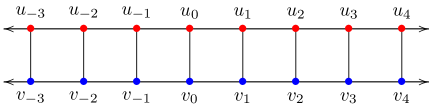
Figure 1: The picture shows the ladder configuration. Red dots on the top side of the ladder correspond to wave function $u_{n}$ and to a linear gain potential $+i\gamma$. Blue dots on the bottom side of the ladder correspond to the wave function $v_{n}$ and to a linear loss potential $-i\gamma$. Vertical lines denote coupling with coefficient $\kappa$ across the rungs of the ladder. Note that the real parts of the linear potential, $U_{n}$ and $V_{n}$, are nonzero only at $n=1,2$.

Figure 2: (Color online) Stationary-solution profiles of $|u|^{2},|v|^{2}$ (black, red) for $\gamma=0.1$, $\kappa=0.6$, $\varepsilon=0.25$, $V_{0}=1$, $T_{1,u}=0.2$, $T_{2,u}=0.8$, $K_{2}=\pi/2$ (top row), $K_{2}=-\pi/2$ (bottom row), in the linear system ($\lambda=0$) with the total ladder length of $200$ for each of $u,v$. Amplitudes $R_{0,u},R_{u},S_{0,u},S_{u}$ are obtained by solving the linear system (7) for $n=1,2$.

Figure 3: (Color online) The nonlinear version of Fig. 2, with $\lambda=1$.

Figure 4: (Color online) The rectification factor $f$ in equation (11) with $t$ defined as per Eq. (9), its nonzero values indicating the non-reciprocity. If $t$ is computed, instead, as per Eq. (10), the plot of $f$ is visually indistinguishable from the above plot. The parameters are $\lambda=1$, $\gamma=0.1$, $\kappa=0.6$, $\varepsilon=0.25$, $K_{1}=\pi/2$, $V_{0}=1$, $\Delta T_{1,u}=\Delta T_{2,u}=0.025$.

Figure 5: (Color online) Stationary-solution profiles of $|u|^{2},|v|^{2}$ (black, red) with $K_{2}$ real and $K_{1}$ complex. The parameters are $q=-1.8$, $\gamma=0.8$, $\kappa=1$, $\varepsilon=0.2$, $V_{0}=1$, $R_{0,u}=0$, $S_{0,u}=3$, and $\lambda=0$. Amplitudes $T_{1,u}$, $R_{u},T_{2,u}$, $S_{u}$ are obtained by solving linear system (7) for $n=1,2$. For the top plot $K_{1}\approx\pi+0.62i,K_{2}\approx 2.21$ are determined by Eq. (4) and for the bottom plot $K_{1}\approx-(\pi+0.62i),K_{2}\approx-2.21$. Here the lattice length is $200$.

In fact, one can introduce the initial ansatz so that Eq. (8) holds only for the sites $n<1$ and $n>2$, i.e., in the linear parts of the system. Then, plugging the so restricted ansatz into Eq. (7) shows that the full expression (8) follows as a consequence. In other words, the format of the ansatz applies at $n=1$ and $n=2$ if one originally defines it solely at $n<1$ and $n>2$.

For each of the summands in Eq. (8), the relation between the amplitudes in the form of Eq. (5) applies. Namely, amplitude pairs $\{A,B\}=\{R_{0,u},R_{0,v}\}$, $\{R_{u},R_{v}\}$, $\{T_{1,u},T_{1,v}\}$ with $K_{1}$ satisfy Eq. (5) with the upper (minus) sign, while amplitude pairs $\{A,B\}=\{S_{0,u},S_{0,v}\}$, $\{S_{u},S_{v}\}$, $\{T_{2,u},T_{2,v}\}$ with $K_{2}$ satisfy Eq. (5) with the lower (plus) sign. In other words, all amplitudes of $\psi$ can be computed in terms of the amplitudes of $\phi$. We consider $q,\kappa,\gamma$ as control parameters, $K_{1},K_{2}$ being computed via Eq. (4). To determine the amplitudes in the stationary solution in the form of Eq. (8), one begins by eliminating all the $\psi$ amplitudes in favor of their $\phi$ counterpart, as per the above relations. Then, specifying values for two out of the six $\phi$ amplitudes, we solve the equations for the remaining four $\phi$ amplitudes using four equations (7) at $n=1,2$. In the linear case ($\lambda=0$), this yields four complex linear equations. In the nonlinear case, with $\lambda\neq 0$, the equations are linear only if $|\phi_{1}|^{2},|\psi_{1}|^{2},|\phi_{2}|^{2},|\psi_{2}|^{2}$ are known. In other words, in the nonlinear case we first compute the input as a function of the transmitted output by specifying the two $\phi$ amplitudes, $T_{1,u}$ and $T_{2,u}$, and then solve for the remaining four $\phi$ amplitudes $R_{0,u},R_{u},S_{0,u},S_{u}$. In the linear case, one may either compute the input as a function of the output, like in the nonlinear case, or first specify the input, $R_{0,u}$ and $S_{0,u}$, and subsequently use Eq. (7) at $n=1,2$ to solve for the output, viz., $R_{u},S_{u},T_{1,u},T_{2,u}$. The so obtained sample profiles in the linear and nonlinear cases are shown in Figs. 2 and 3.

For the solution in the form of Eq. (8), the transmission coefficient can be defined either locally,

$$t=\frac{|T_{1,u}|^{2}+|T_{2,u}|^{2}}{|R_{0,u}|^{2}+|S_{0,u}|^{2}},$$ (9)

or globally,

$$t=\frac{\displaystyle\sum_{n\geq 3}|T_{1,u}e^{iK_{1}n}+T_{2,u}e^{iK_{2}n}|^{2}}{\displaystyle\sum_{n\leq 0}|R_{0,u}e^{iK_{1}n}+S_{0,u}e^{iK_{2}n}|^{2}}.$$ (10)

To address the reciprocity of the transmission, we then define the rectification factor as

$$f=\frac{t(K_{1},K_{2},A,B)-t_{\mathrm{flip}}(K_{1},K_{2},A,B)}{t(K_{1},K_{2},A,B)+t_{\mathrm{flip}}(K_{1},K_{2},A,B)},$$ (11)

where $A,B$ is $T_{1,u},T_{2,u}$ in the case when the input is computed as a function of the output, or $A,B$ is $R_{0,u},S_{0,u}$ in the case when the output is computed as a function of the input. The $t_{\mathrm{flip}}$ notation indicates that the solution was computed with the potentials $U,V$ flipped across the midpoint between the $n=1,2$ sites. This is equivalent to a solution with both $K_{1},K_{2}$ negative. Figure 4 shows a plot of $f$ as a function of $T_{1,u},T_{2,u}$ to demonstrate non-reciprocity of the nonlinear system. Similar to what has been previously observed for the Hamiltonian nonlinear asymmetric chains in Ref. [29, 32], and for the single $\mathcal{PT}$-symmetric chain in Ref. [18], the transmission asymmetry is evident. It is worthy to note that there appears a set of near-unity values of the output-wave parameters, $T_{1,u}$ and $T_{2,u}$, for which this asymmetry is most pronounced.

If $\varepsilon=0$, i.e., the skew part is absent in potential (2), then the $K_{1},K_{2}$ branches are decoupled in the following sense. Setting $S_{0,u}=0$ and $R_{0,u}\neq 0$ gives solutions for the remaining amplitudes such that $T_{1,u},R_{u}\neq 0$ and $T_{2,u},S_{u}=0$. In other words, if the $K_{1}$ branch is present, while $K_{2}$ is absent in the incident part of the wave, then only $K_{1}$ will be present in the reflected and transmitted waves. The same is true for $K_{2}$ if it is originally present while $K_{1}$ is not. For $\varepsilon=0$, the results demonstrate the reciprocity in the linear case $(\lambda=0)$, so that $f$ defined as per Eq. (11) is always zero, for $t$ defined either as in Eq. (9) or as in Eq. (10).

If $\varepsilon\neq 0$, then the $K_{1},K_{2}$ branches are coupled, hence setting $S_{0,u}=0$ and $R_{0,u}\neq 0$ gives solutions for the remaining amplitudes such that $T_{1,u},R_{u},T_{2,u},S_{u}\neq 0$. In other words, if the $K_{1}$ branch is present and $K_{2}$ is absent in the incident part of the wave, then both $K_{1},K_{2}$ will appear in the reflected and transmitted parts of the wave. The same is naturally also true if $K_{2}$ is incident in the absence of $K_{1}$.

Thus far we have considered extended wave solutions in the form of Eq. (8) with real $K_{1},K_{2}$ satisfying Eq. (4). Such solutions also exist in the case when one of $K_{1},K_{2}$ is real and one is complex. As follows from Eq. (4), this happens when one of the expressions $\frac{1}{2}(q\mp\sqrt{\kappa^{2}-\gamma^{2}})$ is in the interval $(-1,1)$, while the other one is not. If $K\equiv x+iy$ with real $x$ and $y$ is the complex wavenumber (either $K_{1}$ or $K_{2}$), then we can write $\cos K=\cos x\cdot\cosh y-i\sin x\cdot\sinh y$. From Eq. (4) we also have that $\sqrt{\kappa^{2}-\gamma^{2}}=\cos(K_{1})-\cos(K_{2})$ is real. From here it follows that $x$ is a multiple of $\pi$ so that $\cos K$ is real, and $y=\pm\mathrm{\ Arcosh}(|\cos\left(K\right)|)$ . The positive value of $y$ allows for solutions in the form given by Eq. ( 8) to stay finite as $n\rightarrow\pm\infty$ (i.e., the wave with complex $K$ is a localized one). In this case, one must set, at $\infty$, the incident amplitude associated with $K$ equal to zero ($S_{0,u}=0$ if $K=K_{2}$ or $R_{0,u}=0$ if $K=K_{1}$). Since both branches are generated when one branch is represented by the incident wave, the complex-$K$ contribution will appear in the reflected and transmitted parts. Figure 5 shows a sample profile of such a physically relevant solution with complex $K_{1}$.

3.2 Stability

To analyze the stability of the plane wave solutions we set $\{u_{n},v_{n}\}\equiv\{e^{iqz}(\phi_{n}+\delta\Phi_{n}(z)),e^{iqz}(\psi_{n}+\delta\Psi_{n}(z))\}$ where $\phi_{n},\psi_{n}$ are stationary solutions of (7) in the form of (8) as described in Section III.A and $\delta>0$ is small. Writing $\Psi_{n}=a_{n}e^{i\nu t}+b_{n}^{*}e^{-i\nu^{\ast}t}$ and $\Phi_{n}=c_{n}e^{i\nu t}+d_{n}^{*}e^{-i\nu^{\ast}t}$ gives the linear system

$$M\left[\begin{array}[]{c}a_{n}\\ b_{n}\\ c_{n}\\ d_{n}\end{array}\right]=\nu\left[\begin{array}[]{c}a_{n}\\ b_{n}\\ c_{n}\\ d_{n}\end{array}\right]$$ (12)

with the nonzero entries of the $M$ matrix as follows

$$M_{11} = diag(-q-i\gamma-U_{n}-2\alpha_{n}|u_{n}|^{2})+G$$

$$M_{22} = diag(q-i\gamma+U_{n}+2\alpha_{n}|u_{n}|^{2})-G$$

$$M_{33} = diag(-q+i\gamma-V_{n}-2\alpha_{n}|v_{n}|^{2})+G$$

$$M_{44} = diag(q+i\gamma+V_{n}+2\alpha_{n}|v_{n}|^{2})-G$$

$$M_{12} = -diag(\alpha_{n}u_{n}^{2})=-M_{21}^{*}$$

$$M_{34} = -diag(\alpha_{n}v_{n}^{2})=-M_{43}^{*}$$

$$M_{24} = M_{42}=diag(\kappa)=-M_{13}=-M_{31}$$ (13)

where $\alpha_{n}=\lambda\left(\delta_{n,1}+\delta_{n,2}\right)$ and $G$ is a sparse matrix with ones on the super- and sub-diagonals. A stationary solution $\phi_{n},\psi_{n}$ is then stable if $max(Re(i\nu))>0$. Figure 6 shows the stability calculation as a function of the output amplitudes $T_{1,u},T_{2,u}$ for stationary solutions according to Section III.A. As expected, one sees a higher strength of instability for higher values of $\gamma,\varepsilon$. A typical example of an unstable plane wave solution is shown in Figure 7 with a corresponding eigenvalue/eigenvector pair and some snapshots of the propagation in time. As time increases the amplitude of the unstable solution concentrates on one of the nonlinear nodes on the $u$-side of the ladder, i.e. on the gain side. This behaviour is consistent with previous results [17, 18].

Figure 6: (Color online) Plots of $max(Re(i\nu))$ as a function of $T_{1,u},T_{2,u}$ indicating the (in)-stability of the plane wave solutions that are computed as described in Section III.A. Parameter values in each panel are: $\gamma=\varepsilon=0$ (top left), $\gamma=0$ and $\varepsilon=0.25$ (top right), $\gamma=0.1$ and $\varepsilon=0$ (bottom left), and $\gamma=\varepsilon=0.1$. All panels have values $K_{1}=\pi/2,\lambda=1,\kappa=0.6,V_{0}=1$, and total ladder length of $200$.

Figure 7: (Color online) The top panel shows the stationary state $|\psi|^{2},|\phi|^{2}$ (black, red) for parameter values $\kappa=0.6,\gamma=0.1,\varepsilon=0.1,T_{1,u}=0.1,T_{2,u}=0.2$. The solution is unstable and $i\nu$ is plotted in the complex plane in the right panel of the second row where $\nu$ are eigenvalues of $M$ in (13). An unstable eigenvector is plotted in the left panel of the second row. The third and fourth rows show the evolution in time of the solution when perturbed in the direction of the eigenvector at $t=5$ and $t=25$. For the wave function plots, blue corresponds to $u$ and green to $v$.

4 Dynamical simulation of the wave-packet scattering

We now turn to the scattering of finite-size wave packets on the central core of the system, which is, obviously, another problem of physical interest. We have performed simulations for the chains of finite lengths, i.e., for $|n|\leq M$ (this means that each of the two chains is composed of $2M+1$ sites). Open boundary conditions are enforced on both chains, namely $u_{-M-1}=u_{M+1}=0$ and $v_{-M-1}=v_{M+1}=0$. Initial conditions were taken as a Gaussian wave packet, with the center placed at point $n_{0}<0$:

$$\left(\begin{array}[]{c}u_{n}(0)\\ v_{n}(0)\end{array}\right)=\left(\begin{array}[]{c}A\\ B\end{array}\right)\exp\left(-\frac{\left(n-n_{0}\right)^{2}}{w}-iKn\right),$$ (14)

where width $w$ is large enough, with respect to the typical wavelength. Initial amplitudes $A$ and $B$ are chosen according to Eq. (5). The pulse created in the form of Eq. (14) will thus be traveling with the group velocity determined by dispersion relation (4):

$$c_{\mathrm{gr}}=-\frac{dq}{dK}=2\sin K.$$ (15)

To understand the results, it is necessary to keep in mind that, as matter of fact, we create a mixture of two modes that correspond, according to dispersion relation (4), to the same $K$, with equal group velocities (15). Such a compound pulse will be traveling as a whole, featuring internal intra-chain oscillations at the spatial beating frequency

$$K_{\mathrm{beat}}=\pi/\sqrt{\kappa^{2}-\gamma^{2}},$$ (16)

as it follows from Eq. (4).

Here we report typical results of the simulations with initial condition ( 14). To minimize the dispersive effects and, thus, the dependence of the scattering on the initial position $n_{0}$, we focus here on the case of $K=\pi/2$. Moreover, for given lattice size $M$, the simulation duration $z_{\mathrm{fin}}$ is limited so as to avoid the hitting of the boundary sites by the transmitted and reflected packets. Then, the wavepacket-transmission coefficients for the two coupled chains, produced by the simulations in the interval of $0<z<z_{\mathrm{fin}}$, are naturally defined as

$$t_{u}=\frac{\sum_{n>n_{\ast}}|u_{n}(z_{\mathrm{fin}})|^{2}}{\sum_{n<1}(|u_{n}(0)|^{2}+|v_{n}(0)|^{2})},$$ (17)

$$t_{v}=\frac{\sum_{n>n_{\ast}}|v_{n}(z_{\mathrm{fin}})|^{2}}{\sum_{n<1}(|u_{n}(0)|^{2}+|v_{n}(0)|^{2})},$$ (18)

the total transmission being $t=t_{u}+t_{v}$. However, a problem with this definition is that the power in the rightmost region may grow, due to the contribution from the region near the central core, where the waves may be trapped and amplified by the gain term, because the nonlinearity may break its balance with the loss. To avoid this, we measure the transmitted power far from the center in a “moving window” containing all the transmitted power, but excluding the trapped fraction localized around $n=1,2$. This is accomplished by extending the sums in Eqs. (17) and (18) to the region of $n>n_{\ast}$, with $n_{\ast}=c_{\ast}z+m$, where $c_{\ast}$ is equal to or smaller than the group velocity $c_{\mathrm{gr}}$ ( $c_{\ast}=1.8$ is fixed henceforth), and $m$ is a suitable constant.

In Figs. 8 and 10, we display results of the nonlinear system for different values of $\gamma$. In addition to the transmission/reflection of the wavepacket, for $\gamma\neq 0$ we also observe an “after-effect” on the central sites of the ladder, $n=1,2$, after the collision with the localized wavepacket. The sites break the balance between the gain and loss, inducing the growth of the power at the gain-carrying sites. The growth does not stay localized at $n=1,2$, but rather expands to additional rungs of the ladder.

Figure 8: (Color online) Numerical simulations of the transmission of Gaussian wavepackets for three values of the gain coefficient, $\gamma=0$, $0.05$ and $0.08$ (from top to bottom). Parameters are $\lambda=1$, $V_{0}=-2.5$, $\kappa=0.1$, $K=\pi/2$, $\varepsilon=0.05$, $M=2000$, $|A|^{2}=2$, $w=20$ and $n_{0}=-250$.

To monitor the effect of the interplay of the nonlinearity with the gain and loss in the system, in the left panels of Fig. 9 we display the evolution at the central sites. As $\gamma$ increases, the power attains large values at these sites. The right panels show the transmission as a function of evolution variable $t_{u,v}(z_{\mathrm{fin}})$, avoiding the growing part, as described above. Note that these panels clearly demonstrate the expected oscillations at the beating frequency given by Eq. (16).

Figure 9: (Color online) Simulations of the wave-packet scattering for increasing gain strength $\gamma$, with other parameters as in the previous figure. Left panels: the evolution of the norm at the central site. Right panels: the evolution of the transmitted intensities as defined by Eqs. (17) and (18). Note the steep growth of $|u_{1}|^{2}$ observed in the left-bottom panel; outside the displayed window $|u_{1}|^{2}$ continues to grow.

Next we address the issue of the asymmetric (non-reciprocal) transmission. This is done by comparing the scattering for the same packet impinging on the nonlinear core from the opposite direction. A noteworthy effect is seen in that regard in Fig. 11, where we compare increasing values of the nonlinearity coefficient $\lambda$ (this is of course equivalent to raising the input power). For moderate values ($\lambda=0.75$, in the left panels of Fig. 11), reciprocity violations in the transmitted intensities are manifest, as the outgoing pulses are different in their shape and intensity. An important manifestation of the non-reciprocity is that some energy remains trapped by the central segment only for the right-incoming packets, but not for the left-incoming ones (which, in turn, feature a stronger transmission). For a larger nonlinearity, $\lambda=1.0$ (right panels in Fig. 11), some power remains trapped in both cases, although the amounts are different. In this case too, the left-incoming packets feature a larger amount of the transmission, while the right-incoming exhibit a considerably weaker transmission and a larger trapping fraction.

Figure 10: (Color online) Spacetime plots of numerical simulations of the transmission of Gaussian wavepackets for moderate and large nonlinearities, $\lambda=0.75$ (top two rows) and $\lambda=1.0$ (bottom two rows). Parameters are $\kappa=0.6$, $\gamma=0.1$, $V_{0}=-2.5$, $K=\pi/2$, $\varepsilon=0.25$, $M=2000$, $|A|^{2}=1$, $w=100$ and $n_{0}=-500$.

Figure 11: (Color online) Profiles of the Gaussian wavepackets at a time after the packet has interacted with the nonlinear core. Parameter values are the same as those in Figure 11. Note that the horizontal axis for the data referring to the right-incoming packets have been mirror-reversed to facilitate the comparison with the left-incoming ones

5 Conclusions

We have introduced and examined a ladder system with the $\mathcal{PT}$ -balanced combination of gain and loss uniformly distributed along the pair of parallel chains, which are linearly coupled in the transverse direction, and the core part, localized at two central sites, which carry the linear potential and onsite nonlinearity. Two branches of plane-wave solutions were found. The branches are mixed at the central core if the potential functions are skew-symmetric [$\varepsilon\neq 0$ in Eq. (2)], and they stay uncoupled for $\varepsilon=0$. In the former case, asymmetric transmission is observed, and is quantified by means of the rectification factor, $f$, defined as per Eq. (11). We have also performed simulations of the interaction of incident Gaussian wavepackets with the embedded core, similarly observing the asymmetry of the transmission in the presence the nonlinearity at the central sites. This asymmetry was quantified by suitable transmissivities, and characteristic features of the evolution of right- and left-incoming wavepackets were clarified through the direct simulations.

As regards future work, it would be particularly relevant to explore generalizations of the present settings to fully two-dimensional lattices, a topic that has received relatively limited attention in the realm of $\mathcal{PT}$-symmetric systems (see, e.g., Refs. [34, 35] for some recent examples). Another relevant possibility is to consider, instead of the “straight” ladder, with one chain carrying the gain and the other – the loss, an “alternating” ladder, where the gain-loss rungs would alternate with their loss-gain counterparts , i.e., each gain node would be coupled to three neighbors bearing the loss, and vice versa. Such settings are currently under examination and will be presented in future publications.

References

- [1]
- [2]
- [3]
- [4]
- Kosevich [1995] Y. A. Kosevich, Phys. Rev. B 52, 1017 (1995).
- Liang et al. [2009] B. Liang, B. Yuan, and J. chun Cheng, Phys. Rev. Lett. 103, 104301 (2009).
- Liang et al. [2010] B. Liang, X. Guo, J. Tu, D. Zhang, and J. Cheng, Nature Materials 9, 989 (2010), ISSN 1476-1122.
- Nesterenko et al. [2005] V. F. Nesterenko, C. Daraio, E. B. Herbold, and S. Jin, Phys. Rev. Lett. 95, 1 (2005).
- Boechler et al. [2011] N. Boechler, G. Theocharis, and C. Daraio, Nature Materials 10, 665 (2011).
- Scalora et al. [1994] M. Scalora, J. P. Dowling, C. M. Bowden, and M. J. Bloemer, J. Appl. Phys. 76, 2023 (1994).
- Tocci et al. [1995] M. D. Tocci, M. J. Bloemer, M. Scalora, J. P. Dowling, and C. M. Bowden, Appl. Phys. Lett. 66, 2324 (1995).
- Gallo et al. [2001] K. Gallo, G. Assanto, K. Parameswaran, and M. Fejer, Appl. Phys. Lett. 79, 314 (2001).
- Feise et al. [2005] M. W. Feise, I. V. Shadrivov, and Y. S. Kivshar, Phys. Rev. E 71, 037602 (2005).
- Konotop and Kuzmiak [2002] V. V. Konotop and V. Kuzmiak, Phys. Rev. B 66, 235208 (2002).
- Biancalana [2008] F. Biancalana, J. Appl. Phys. 104, 093113 (2008).
- Grigoriev and Biancalana [2011] V. Grigoriev and F. Biancalana, Opt. Lett. 36, 2131 (2011).
- Ramezani et al. [2010] H. Ramezani, T. Kottos, R. El-Ganainy, and D. N. Christodoulides, Phys. Rev. A 82, 043803 (2010).
- D’Ambroise et al. [2012] J. D’Ambroise, P. G. Kevrekidis, and S. Lepri, J. Phys. A: Math. Theor. 45, 444012 (2012).
- [19] N. Bender, S. Factor, J. D. Bodyfelt, H. Ramezani, D. N. Christodoulides, F. M. Ellis, and T. Kottos, Phys. Rev. Lett. 110, 234101 (2013).
- Roy [2010] D. Roy, Phys. Rev. B 81, 155117 (2010).
- Tao et al. [2011] F. Tao, W. Chen, W. Xu, J. Pan, and S. Du, Phys. Rev. E 83, 056605 (2011).
- Eilbeck et al. [1985] J. C. Eilbeck, P. S. Lomdahl, and A. C. Scott, Physica D 16, 318 (1985).
- Kevrekidis [2009] P. G. Kevrekidis, The Discrete Nonlinear Schrödinger Equation (Springer Verlag, Berlin, 2009).
- Brazhnyi and Malomed [2011] V. Brazhnyi and B. A. Malomed, Phys. Rev. A 83, 053844 (2011).
- Molina and Tsironis [1993] M. I. Molina and G. P. Tsironis, Phys. Rev. B 47, 15330 (1993).
- Gupta and Kundu [1997a] B. C. Gupta and K. Kundu, Phys. Rev. B 55, 894 (1997a).
- Gupta and Kundu [1997b] B. C. Gupta and K. Kundu, Phys. Rev. B 55, 11033 (1997b).
- Bulgakov et al. [2011] E. Bulgakov, K. Pichugin, and A. Sadreev, Phys. Rev. B 83, 045109 (2011).
- Lepri and Casati [2011] S. Lepri and G. Casati, Phys. Rev. Lett. 106, 164101 (2011).
- [30] S. Lepri and G. Casati. ”Nonreciprocal wave propagation through open, discrete nonlinear Schrödinger dimers.” in ”Localized Excitations in Nonlinear Complex Systems: Current State of the Art and Future Perspectives”, in: R. Carretero-González, J. Cuevas-Maraver, D. Frantzeskakis, N. Karachalios, P. Kevrekidis, F. Palmero-Acebedo (Eds.) Springer Series: Nonlinear Systems and Complexity, Vol. 7 (2014).
- [31] Y. Li, J. Zhou, F. Marchesoni, and B. Li, Scientific Reports, 4 4566 (2014).
- Lepri and Malomed [2013] S. Lepri and B. A. Malomed, Phys. Rev. E 87, 042903 (2013).
- [33] S. V. Dmitriev, S. V. Suchkov, A. A. Sukhorukov, and Y. S. Kivshar, Phys. Rev. A 84, 013833 (2011); S. V. Suchkov, A. A. Sukhorukov, S. V. Dmitriev, and Y. S. Kivshar, EPL 100, 54003 (2012); S. V. Suchkov, S. V. Dmitriev, B. A. Malomed, and Y. S. Kivshar, Phys. Rev. A 85, 033835 (2012); D. A. Zezyulin, and V. V. Konotop, Phys. Rev. Lett. 108, 213906 (2012); A. Regensburger, M. A. Miri, C. Bersch, J. Näger, Phys. Rev. Lett. 110, 223902 (2013).
- [34] V. Achilleos, P. G. Kevrekidis, D. J. Frantzeskakis, and R. Carretero-González, Phys. Rev. A 86, 013808 (2012).
- [35] B. Midya, arXiv:1404.7322.