Optimized Schwarz Waveform Relaxation for
Advection Reaction Diffusion Equations in Two Dimensions

Abstract

Optimized Schwarz Waveform Relaxation methods have been developed over the last decade for the parallel solution of evolution problems. They are based on a decomposition in space and an iteration, where only subproblems in space-time need to be solved. Each subproblem can be simulated using an adapted numerical method, for example with local time stepping, or one can even use a different model in different subdomains, which makes these methods very suitable also from a modeling point of view. For rapid convergence however, it is important to use effective transmission conditions between the space-time subdomains, and for best performance, these transmission conditions need to take the physics of the underlying evolution problem into account. The optimization of these transmission conditions leads to mathematically hard best approximation problems of homographic functions. We study in this paper in detail the best approximation problem for the case of linear advection reaction diffusion equations in two spatial dimensions. We prove comprehensively best approximation results for transmission conditions of Robin and Ventcel (higher order) type, which can also be used in the various limits for example for the heat equation, since we include in our analysis a positive low frequency limiter both in space and time. We give for each case closed form asymptotic values for the parameters which can directly be used in implementations of these algorithms, and which guarantee asymptotically best performance of the iterative methods. We finally show extensive numerical experiments including cases not covered by our analysis, for example decompositions with cross points. In all cases, we measure performance corresponding to our analysis.

Keywords Domain decomposition, waveform relaxation, best approximation.

2010 Mathematics Subject Classification 65M55, 65M15.

1 Introduction

Schwarz waveform relaxation algorithms are parallel algorithms to solve evolution problems in space time. They were invented independently in [20] and [24], see also [21], based on the earlier work in [4], and are a combination of the classical waveform relaxation algorithm from [32] for the solution of large scale systems of ordinary differential equations, and Schwarz methods invented in [39]. Modern Schwarz methods are among the best parallel solvers for steady partial differential equations, see the books [40, 38, 41] and references therein. Waveform relaxation methods have been analyzed for many different classes of problems recently: for fractional differential equations see [30], for singular perturbation problems see [47], for differential algebraic equations see [2], for population dynamics see [23], for functional differential equations see [48], and especially for partial differential equations, see [28, 29, 43] and the references therein. For the particular form of Schwarz waveform relaxation methods, see [6, 18, 8, 7, 31, 46, 22, 35, 5, 45, 33, 34]. These algorithms have also become of interest in the moving mesh R-refinement strategy, see [27, 26, 17], and references therein.

Schwarz waveform relaxation methods however exhibit only fast convergence, when optimized transmission conditions are used, as first shown in [16], and then treated in detail in [36, 15, 3, 42] for diffusive problems, and [10, 9] for the wave equation, see also [19, 14] for circuit problems, and [1] for the primitive equations. With optimized transmission conditions, the algorithms can be used without overlap, and optimized transmission conditions turned out to be important also for Schwarz algorithms applied to steady problems, for an overview, see [11] and references therein. In order to make such algorithms useful in practice, one needs simply to use formulas for the optimized parameters, which can then be put into implementations and lead to fast convergent algorithms, without having to think about optimizing transmission conditions ever again.

The purpose of this paper is to provide such formulas for a general evolution problem of advection reaction diffusion type. The analysis required to solve the associated optimization problems is substantial, and only asymptotic techniques lead to easy to use, closed form formulas. We also use and extend more general, abstract results for best approximation problems, which appeared in [3]. In particular, we remove a compactness condition which remained in [3] in the case of overlap. We obtain with our analysis the best choice of Robin transmission conditions, and also higher order transmission conditions called Ventcel conditions (after the Russian mathematician A. D. Ventcel, also spelled Venttsel, Ventsel or Wentzell [44]), both for the case of overlapping and non-overlapping algorithms. We give complete proofs of optimality, generalizing one-dimensional results given in [15] and [3]. We also illustrate our results with numerical experiments.

2 Model Problem and Main Results

We study the optimized Schwarz waveform relaxation algorithm for the time dependent advection reaction diffusion equation in $\Omega\subset\mathbb{R}^{2}$,

$$\mathcal{L}u:=\partial_{t}u+\mbox{\boldmath$a$}\cdot\nabla u-\nu\Delta u+bu=f,\quad\mbox{in $\Omega\times(0,T)$,}$$ (2.1)

where $\nu>0$, $b\geqslant 0$ and $\mbox{\boldmath$a$}=(a,c)^{T}$, and suitable boundary conditions need to be prescribed on the boundary of $\Omega$, which will however not play an important role, and we will not mention this further. In order to describe the Schwarz waveform relaxation algorithm, we decompose the domain into J non-overlapping subdomains $U_{j}$, and then enlarge them, if desired, in order to obtain an overlapping decomposition given by subdomains $\Omega_{j}$. The interfaces between subdomain $\Omega_{i}$ and $\Omega_{j}$ are then defined by $\Gamma_{ij}=\partial\Omega_{i}\cap\overline{U}_{j}$. The algorithm for such a decomposition calculates then for $n=1,2,\ldots$ the iterates $(u_{j}^{n})$ defined by

$$\begin{array}[]{rcl}\mathcal{L}u_{i}^{n}&=&f\quad\mbox{in $\Omega_{i}\times(0,T)$}\\ u_{i}^{n}(\cdot,\cdot,0)&=&u_{0}\quad\mbox{in $\Omega_{i}$},\\ \mathcal{B}_{ij}u_{i}^{n}&=&\mathcal{B}_{ij}u_{j}^{n-1}\mbox{ on $\Gamma_{ij}\times(0,T)$},\end{array}$$ (2.2)

where the $\mathcal{B}_{ij}$ are linear differential operators in space and time, and initial guesses $\mathcal{B}_{ij}u_{j}^{0}$ on $\Gamma_{ij}\times(0,T)$ need to be provided.

There are many different choices for the operators ${\cal B}_{ij}$. Choosing for ${\cal B}_{ij}$ the identity leads to the classical Schwarz waveform relaxation method, which needs overlap for convergence. Zeroth or higher order differential conditions lead to optimized variants, which also converge without overlap, see for example [15] and [3], where a complete analysis in one dimension was performed. We study here in detail the case where the transmission operators are of the form

$${\cal B}_{ij}=(\nu\nabla-\frac{\mbox{\boldmath$a$}}{2})\cdot\mbox{\boldmath$n_{i}$}+\frac{s}{2},\qquad s=p+q(\partial_{t}+c\partial_{y}-\nu\Delta_{y}).$$ (2.3)

If $q=0$, these are Robin transmission conditions, whereas for $q\neq 0$, they are called Ventcel transmission conditions. In the ideal case where $\Omega=\mathbb{R}^{2}$ is decomposed into two half spaces $\Omega_{1}=(-\infty,L)\times\mathbb{R}$ and $\Omega_{2}=(0,\infty)\times\mathbb{R}$, we can compute explicitly the error in each subdomain at step $n$ as a function of the initial error. We use Fourier transforms in time and in the direction $y$ of the boundary, with $\omega$ and $k$ the Fourier variables. The convergence factor $\rho(\omega,k,p,q,L)$ of algorithm (2.2), which gives precisely the error reduction of each error component in $\omega$ and $k$ for a given choice of parameters $p$ and $q$ and overlap $L$, can in this case be computed in closed form (see [15]),

$$\rho(\omega,k,p,q,L)=\frac{p+q(\nu k^{2}+i(\omega+ck))-\sqrt{x_{0}^{2}+4\nu(\nu k^{2}+i(\omega+ck))}}{p+q(\nu k^{2}+i(\omega+ck))+\sqrt{x_{0}^{2}+4\nu(\nu k^{2}+i(\omega+ck))}}e^{-\frac{L\sqrt{x_{0}^{2}+4\nu(\nu k^{2}+i(\omega+ck))}}{2\nu}},$$ (2.4)

where we denote by $\sqrt{\ }$ the standard branch of the square root with positive real part, $x_{0}^{2}:=a^{2}+4\nu b$ and $i=\sqrt{-1}$. Computing on a (uniform) grid, we assume that the maximum frequency in space is $k_{M}=\frac{\pi}{h}$ where $h$ is the local mesh size in $x$ and $y$, and the maximum frequency in time is $\omega_{M}=\frac{\pi}{\Delta t}$, and that we also have estimates for the lowest frequencies $k_{m}$ and $\omega_{m}$ from the geometry, see for example [11] for estimates, or for a more precise analysis see [13]. We also assume that the mesh sizes in time and space are related either by $\Delta t=C_{h}h$, or $\Delta t=C_{h}h^{2}$, corresponding to a typical implicit or explicit time discretization of the problem.

Defining $D:=\{(\omega,k),\omega_{m}\leqslant|\omega|\leqslant\omega_{M},\,k_{m}\leqslant|k|\leqslant k_{M}\}$, the parameters $(p^{*},q^{*})$ which give the best convergence factor are solution of the best approximation problem

$$\inf_{(p,q)\in\mathbb{C}^{2}}\ \sup_{(\omega,k)\in D}|\rho(\omega,k,p,q,L)|=\sup_{(\omega,k)\in D}|\rho(\omega,k,p^{*},q^{*},L)|=:\delta^{*}(L).$$ (2.5)

To motivate the reader, we outline in Table 1 the asymptotic behavior of the convergence factors, which can be achieved by optimization. We use here the notation $Q\backsimeq h$ or $Q=\varpropto\!\!(h)$ if there exists $C\neq 0$ such that $Q\sim Ch$.

Method	No overlap	Overlap $L$
Dirichlet	1	$1-\varpropto\!\!(L)$
Robin	$1-\varpropto\!\!(\sqrt{h})$	$1-\varpropto\!\!(\sqrt[3]{L})$
Ventcel	$1-\varpropto\!\!(\sqrt[4]{h})$	$1-\varpropto\!\!(\sqrt[5]{L})$

Table 1: The asymptotically optimized convergence factors $\delta^{*}(L)$.

In what follows, we will often use the quantity

$$\bar{k}=|c|\,\frac{\sqrt{(c^{2}+x_{0}^{2})^{2}+16\nu^{2}\omega_{m}^{2}}-(c^{2}+x_{0}^{2})}{8\nu^{2}\omega_{m}}.$$

By a direct calculation, we see that $0\leqslant\bar{k}|c|\leqslant\omega_{m}$, and we define the function

$$\begin{array}[]{l}\varphi(k,\xi):=2\sqrt{2}\sqrt{\sqrt{(x_{0}^{2}+4\nu^{2}k^{2})^{2}+16\nu^{2}\xi^{2}}+x_{0}^{2}+4\nu^{2}k^{2}},\end{array}$$ (2.6)

and the constant

$$A=\left\{\begin{array}[]{ll}\varphi(\bar{k},-\omega_{m}+|c|\bar{k})&\mbox{if $k_{m}\leqslant\bar{k}$,}\\ \varphi(k_{m},-\omega_{m}+|c|k_{m})&\mbox{if $\bar{k}\leqslant k_{m}\leqslant\frac{1}{|c|}\omega_{m}$,}\\ \varphi(k_{m},0)&\mbox{if $k_{m}\geqslant\frac{1}{|c|}\omega_{m}$.}\\ \end{array}\right.$$ (2.7)

We state in the following two subsections the main theorems which we will prove in this paper, for both overlapping and non-overlapping variants of the algorithm.

2.1 Robin Transmission Conditions

Theorem 2.1 (Robin Conditions without Overlap)

For small $h$ and small $\Delta t$, the best approximation problem (2.5) with $L=0$ has a unique solution $(p_{0}^{*}(0),\delta_{0}^{*}(0))$, which is given asymptotically by

$$p_{0}^{*}(0)\sim\sqrt{\frac{A}{Bh}},\quad\delta^{*}_{0}(0)\sim 1-\frac{1}{2}\sqrt{ABh},$$ (2.8)

where $A$ is defined in (2.7), and

$$B=\left\{\begin{array}[]{ll}\frac{2}{\nu\pi}&\mbox{if $\Delta t=C_{h}h$},\\ C\frac{\sqrt{2d}}{\nu\pi}&\mbox{if $\Delta t=C_{h}h^{2}$, $d:=\nu\pi C_{h}$, $C=\left\{\begin{array}[]{ll}1&\mbox{if $d<d_{0}$},\\ \sqrt{\frac{d+\sqrt{1+d^{2}}}{1+d^{2}}}&\mbox{if $d\geqslant d_{0}$,}\end{array}\right.$}\end{array}\right.$$ (2.9)

where $d_{0}\approx 1.543679$ is the unique real root of the polynomial $d^{3}-2d^{2}+2d-2$.

Partial results in the spirit of this theorem were already obtained earlier:

1. If $k_{m}=\omega_{m}=0$, all three cases in (2.7) coincide, since $\bar{k}=0$, and the constant $A$ simplifies to $A=4x_{0}$, and we find the case analyzed in [25].

2. If $k_{m}$ and $\omega_{m}$ do not both vanish simultaneously, and we are in the case of the heat equation, $a=0$, $b=0$, $c=0$, $\nu=1$, we also obtain $\bar{k}=0$, and $A=4\sqrt{2\left(\sqrt{k_{m}^{4}+\omega_{m}^{2}}+k_{m}^{2}\right)}$, the case analyzed in [42]. Note that the stability constraint for the heat equation discretized with a finite difference scheme is $4\nu\Delta t\leqslant h^{2}$, which with our notation implies that $d\leqslant\pi/4\sim 0.7854$, a value smaller than $d_{0}$, and hence the constant $C$ in (2.9) is equal to 1.

For the algorithm with overlap, $L>0$, we treat two asymptotic cases: the continuous case deals with the small overlap parameter $L$ only, while the discrete case involves also the grid parameters. In the continuous case, we consider the parameters $\omega_{M}$ and $k_{M}$ to be equal to $+\infty$.

Theorem 2.2 (Robin Conditions with Overlap, Continuous)

For small overlap $L>0$, the best approximation problem (2.5) on $D^{\infty}:=\{(\omega,k),\omega_{m}\leqslant|\omega|\leqslant+\infty,\,k_{m}\leqslant|k|\leqslant+\infty\}$ has a unique solution

$$p_{0,\infty}^{*}(L)\sim\frac{1}{2}\sqrt[3]{\frac{\nu A^{2}}{L}},\quad\delta_{0,\infty}^{*}(L)\sim 1-\frac{A}{2p_{0,\infty}^{*}(L)},$$ (2.10)

where $A$ is defined in (2.7).

If the overlap is fixed, the above analysis gives the behavior of the best parameter when $h$ and $\Delta t$ tend to zero. However, the overlap contains in general a few grid points only, and then the discretization also needs to be taken into account:

Theorem 2.3 (Robin Conditions with Overlap, Discrete)

For small $\Delta t$ and $h$, for $L\backsimeq h$, the best approximation problem (2.5) on $D$ has a unique solution

$$\begin{array}[]{ll}\begin{array}[]{rl}\mbox{for $\Delta t\backsimeq h^{2}$}:&p_{0}^{*}(L)\sim p^{*}_{0,\infty}(L),\\ \mbox{for $\Delta t\backsimeq h$}:&p_{0}^{*}(L)\sim\displaystyle\frac{p^{*}_{0,\infty}(L)}{\sqrt[3]{2}},\end{array}&\delta_{0}^{*}(L)\sim 1-\displaystyle\frac{A}{2p_{0}^{*}(L)}.\end{array}$$ (2.11)

2.2 Ventcel Transmission Conditions

In order to present the theorems, we need to define two auxiliary functions: first

$$g(t)=\frac{2t-\sqrt{t^{2}+1}}{t^{2}+1},$$

and we denote for $Q<g_{0}\approx 0.3690$ by $t_{2}(Q)$ the only root of the equation $g(t)=Q$ larger than $t_{0}=\sqrt{54+6\sqrt{33}}/6\approx 1.567618292$. Next we also define

$$P(Q)=\left\{\begin{array}[]{ll}\sqrt{1+\sqrt{t_{2}(Q)^{2}+1}}(\frac{1}{\sqrt{t_{2}(Q)^{2}+1}}+Q)&\mbox{if }Q<g_{1}\approx 0.3148,\\ 1+Q&\mbox{if }Q>g_{1}.\end{array}\right.$$ (2.12)

Theorem 2.4 (Ventcel Conditions without Overlap)

The best approximation problem has for $L~{}=~{}0$ a unique solution $(p_{1}^{*}(0),q_{1}^{*}(0))$, given by

$$\begin{array}[]{llllll}\mbox{for $\Delta t=C_{h}h$ and $\frac{AC_{h}}{8}<1$}:&p_{1}^{*}(0)\sim\frac{1}{2}\sqrt[4]{\frac{\nu\pi A^{3}}{4h}},&\ q_{1}^{*}(0)\sim\frac{8ph}{\pi A},\\ \mbox{for $\Delta t=C_{h}h$ and $\frac{AC_{h}}{8}>1$}:&p_{1}^{*}(0)\sim\sqrt[4]{\frac{\nu\pi A^{2}}{2C_{h}(P(\frac{8}{C_{h}A}))^{2}h}},&q_{1}^{*}(0)\sim\frac{8ph}{\pi A},\\ \mbox{for $\Delta t=C_{h}h^{2}$}:&p_{1}^{*}(0)\sim\frac{1}{2}\sqrt[4]{\frac{\nu\pi A^{3}}{4Ch}\sqrt{\frac{2}{d}}},&q_{1}^{*}(0)\sim\frac{8Cph}{\pi A}\sqrt{\frac{d}{2}},\\[10.00002pt] &\displaystyle\delta_{1}^{*}(0)\sim 1-\displaystyle\frac{A}{2p_{1}^{*}(0)}.&&\end{array}$$ (2.13)

Here again $A$ is the constant defined in (2.7), $d$ and $C$ are the constants defined in (2.9).

Theorem 2.5 (Ventcel Conditions with Overlap, Continuous)

For small overlap $L>0$, the best approximation problem (2.5) on $D^{\infty}$ has the unique solution

$$p_{1,\infty}^{*}(L)\sim\frac{1}{2}\sqrt[5]{\frac{\nu A^{4}}{8L}},\quad q_{1,\infty}^{*}(L)\sim 4\sqrt[5]{\frac{\nu^{2}L^{3}}{2A^{2}}},\quad\delta_{1,\infty}^{*}(L)\sim 1-\displaystyle\frac{A}{2p_{1,\infty}^{*}(L)},$$ (2.14)

where $A$ is defined in (2.7).

Theorem 2.6 (Ventcel Conditions with Overlap, Discrete)

For small $\Delta t$ and $h$, for $L\backsimeq h$, the best approximation problem (2.5) on $D$ has a unique solution

$$\begin{array}[]{ll}\begin{array}[]{rll}\mbox{for $\Delta t\backsimeq h^{2}$}:&p_{1}^{*}(L)\sim p^{*}_{1,\infty}(L),&q_{1}^{*}(L)\sim q^{*}_{1,\infty}(L),\\ \mbox{for $\Delta t\backsimeq h$}:&p_{1}^{*}(L)\sim 2^{-\frac{1}{5}}p^{*}_{1,\infty}(L),&q_{1}^{*}(L)\sim 2^{\frac{3}{5}}q^{*}_{1,\infty}(L),\end{array}&\delta_{1}^{*}(L)\sim 1-\displaystyle\frac{A}{2p_{1}^{*}(L)}.\end{array}$$ (2.15)

3 Abstract Results

We now recall the abstract results on the best approximation problem (2.5) from [3], and present an important extension, which allows us to remove a compactness assumption in the overlapping case. We start by rewriting the convergence factor (2.4) in the form

$$\rho(z,s,L)=\displaystyle\frac{s-z}{s+z}\ e^{-\frac{Lz}{2\nu}},\quad z:=\sqrt{x_{0}^{2}+4\nu(\nu k^{2}+i(\omega+ck))},\quad s=p+q(\nu k^{2}+i(\omega+ck)).$$ (3.1)

In order to separate real and imaginary parts of the square root, we introduce the change of variables ${\mathcal{T}}:(k,\omega)\mapsto z=x+iy$, which transforms the domain $D$ into $\widetilde{D}=\widetilde{D}_{+}\cup\overline{\widetilde{D}_{+}}$, with $\widetilde{D}_{+}\subset\mathbb{R}_{+}\times\mathbb{R}_{+}$, as illustrated in Figure 1.

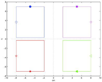
Figure 1: How the change of variables to simplify the convergence factor transforms the frequency domains

The domain $\widetilde{D}_{+}$ is compact, and lies below the line $x=y$, as one can see from the coordinates $(x,y)=(\mathrm{Re}\,{\mathcal{T}}(k,\omega),\mathrm{Im}\,{\mathcal{T}}(k,\omega))$, which satisfy

$$x^{2}-y^{2} = x_{0}^{2}+4\nu^{2}k^{2},$$ (3.2a)

$$2xy = 4\nu(\omega+ck).$$ (3.2b)

We further assume that the coefficients and parameters satisfy

$$\mbox{either\quad$x_{0}^{2}+4\nu^{2}k_{m}^{2}\neq 0$,\quad or\quad$\omega_{m}\neq 0$},$$ (3.3)

which implies that there exists an $\alpha>0$ such that

$$\forall z\in\widetilde{D},\quad\mathrm{Re}\,z\geqslant\alpha>0.$$

We also use the notation $\rho_{0}(z,p,q):=\frac{s-z}{s+z}$, $\rho(z,p,q,L):=\rho_{0}(z,p,q)e^{-Lz/2\nu}$. The min-max problem (2.5) in the new $(x,y)$-coordinates takes now the simple form

$$\inf_{(p,q)\in\mathbb{C}^{2}}\ \sup_{z\in\widetilde{D}}|\rho(z,p,q,L)|=\sup_{z\in\widetilde{D}}|\rho(z,p^{*},q^{*},L)|=:\delta^{*}(L).$$ (3.4)

For convenience, we will also use the notation $R_{0}(\omega,k,p,q)$ or $R_{0}(z,p,q)$ for $|\rho_{0}(z,p,q)|^{2}$, and $R(\omega,k,p,q,L)=R(z,p,q,L)=R_{0}(z,p,q)e^{-Lx/\nu}$.

3.1 Robin Transmission Conditions

In this case, we set $q=0$, and we will simply use the above notation without the parameter $q$ in the arguments, writing for instance $\rho(z,p,L)$, $\rho_{0}(z,p)$, etc.. We also call the minimum in the Robin case $\delta_{0}^{*}(L)$.

We start with the non-overlapping case, $L=0$, where there is a nice geometric interpretation of the min-max problem (3.4): for a given point $z_{o}\in\mathbb{C}$ and a parameter $\delta\in\mathbb{R}$, we introduce the sets

$${\cal C}(z_{0},\delta)=\{z\in\mathbb{C};\ \left|\frac{z-z_{0}}{z+z_{0}}\right|=\delta\},\,\bar{\cal D}(z_{0},\delta)=\{z\in\mathbb{C};\ \left|\frac{z-z_{0}}{z+z_{0}}\right|\leqslant\delta\}.$$ (3.5)

Note that ${\cal C}(z_{0},\delta)$ is a circle centered at $\frac{1+\delta^{2}}{1-\delta^{2}}z_{0}$, cutting the $x-$axis at the points $\frac{1-\delta}{1+\delta}z_{0}$ and $\frac{1+\delta}{1-\delta}z_{0}$, and $\bar{\cal D}(z_{0},\delta)$ is the associated disk. Now because of the form of the convergence factor $\rho_{0}(z,p,q)=\frac{s-z}{s+z}$, $(p^{*},\delta^{*})$ is a solution of the min-max problem (3.4) if and only if for any $z$ in $\widetilde{D}$, $z$ is in $\bar{\cal D}(p^{*},\delta^{*})$. This means geometrically that the solution of the min-max problem (3.4) is represented by the smallest circle centered on the real axis which contains $\widetilde{D}$. We will use this interpretation as a guideline in the analysis, also for the overlapping case!

Theorem 3.1

For any set of coefficients such that (3.3) is satisfied, and $k_{M}$ and $\omega_{M}$ being finite, the min-max problem (3.4) with $L=0$ has a unique solution $(\delta^{*}_{0}(0),p^{*}_{0}(0))$ with $\delta^{*}_{0}(0)<1$. The optimized parameter $p^{*}_{0}(0)$ is real and positive, and any strict local minimum on $\mathbb{R}$ of the real function

$$F_{0}(p)=\sup_{z\in\widetilde{D}_{+}}|\rho_{0}(z,p)|$$ (3.6)

is the global minimum.

Proof  Since $\widetilde{D}$ is compact, and with the assumption (3.3) we have $\mathrm{Re}\,z\geqslant\alpha>0$ with $\alpha=\sqrt{x_{0}^{2}+4\nu^{2}k_{m}^{2}}$ in the first case of (3.3) or $\alpha=\sqrt{2\nu\omega_{m}}$ in the second case, we can use directly the analysis in [3] for polynomials of degree zero to get existence and uniqueness. The fact that the optimized parameter must be real follows directly from the symmetry of $\widetilde{D}$ with respect to the $x$-axis and the geometric interpretation, and finally that any strict local minimum is the global minimum follows as in [3].  

In [3] one can also find a proof of the existence of a solution to the min-max problem (3.4) in the overlapping case, and uniqueness is shown for $L$ small enough, such that

$$\delta^{*}(L)e^{\frac{L}{2\nu}\sup_{z\in\widetilde{D}}\mathrm{Re}\,z}<1.$$

This constraint imposes that $\widetilde{D}$ is bounded in the $x$ direction. We show now that this constraint is not necessary, using the fact that in $\widetilde{D}$ the real part of $z$ is strictly larger than the absolute value of its imaginary part.

Theorem 3.2

For any $L$, for $k_{M}$ and $\omega_{M}$ finite or not, and with the assumption (3.3), the min-max problem (3.4) has a unique solution $(\delta^{*}_{0}(L),p^{*}_{0}(L))$. The optimized parameter $p^{*}_{0}(L)$ is real, positive, and any strict local minimum on $\mathbb{R}$ of the real function

$$F_{L}(p)=\sup_{z\in\widetilde{D}_{+}}|\rho(z,p,L)|$$ (3.7)

is the global minimum.

Proof  By Theorem 2.8 in [3], we know that a (possibly complex) solution $p^{*}=p^{*}_{1}+ip^{*}_{2}$ of (3.4) exists. We now compute explicitly the modulus of the convergence factor,

$$|\rho_{0}(z,p)|^{2}=\displaystyle\frac{(x-p_{1})^{2}+(y-p_{2})^{2}}{(x+p_{1})^{2}+(y+p_{2})^{2}}.$$

We first note that for any $z$, and any $(p_{1},p_{2})$ with $p_{1}>0$, we have $|\rho_{0}(z,-p_{1}+ip_{2})|>|\rho_{0}(z,p_{1}+ip_{2})|$, and therefore we must have $p^{*}_{1}>0$. Next, in order to show that $|p^{*}_{2}|\leqslant p^{*}_{1}$, we assume the contrary, $|p^{*}_{2}|>p^{*}_{1}$, to reach a contradiction (in particular this means that $p^{*}_{2}\neq 0$). We calculate the gradient,

$$\begin{array}[]{l}\partial_{p_{1}}|\rho_{0}(z,p)|^{2}=-4\displaystyle\frac{x(x^{2}+y^{2}+p_{2}^{2}-p_{1}^{2})-2yp_{1}p_{2}}{((x+p_{1})^{2}+(y+p_{2})^{2})^{2}},\\ \partial_{p_{2}}|\rho_{0}(z,p)|^{2}=-4\displaystyle\frac{y(x^{2}+y^{2}+p_{1}^{2}-p_{2}^{2})-2xp_{1}p_{2}}{((x+p_{1})^{2}+(y+p_{2})^{2})^{2}},\end{array}$$

which gives, with $\varepsilon=\mbox{sign}(p^{*}_{2})$,

$$(\partial_{p_{1}}-\varepsilon\partial_{p_{2}})|\rho_{0}(z,p^{*})|^{2}=-4\displaystyle\frac{(x-\varepsilon y)(x^{2}+y^{2}+2\varepsilon p_{1}p_{2})+(x+\varepsilon y)(p_{2}^{2}-p_{1}^{2})}{((x+p_{1})^{2}+(y+p_{2})^{2})^{2}}\,<\,0,$$

where we used the fact that $x>|y|$ as we noted earlier (see Figure 1). This shows that $|\rho_{0}(z,p)|e^{-Lx/2\nu}$ decays in the neighborhood of $p^{*}$, in the direction $(1,-\varepsilon)$, if $|p^{*}_{2}|>p^{*}_{1}$, which is in contradiction with the fact that the minimum is reached, and hence we must have $|p^{*}_{2}|\leqslant p^{*}_{1}$.

Now for any $z$ in $\widetilde{D}$, since $x>|y|$ and $|p^{*}_{2}|\leqslant p^{*}_{1}$, we have

$$\mathrm{Re}\,\frac{p}{z}=\frac{xp^{*}_{1}+yp^{*}_{2}}{|z|^{2}}\,>\,0.$$

This allows us to prove that the set of best approximations is convex: consider the disk defined in (3.5). We have seen that $(p^{*}(L),\delta^{*}(L))$ is a solution of the best approximation problem (3.4), if and only if for any $z$ in $\widetilde{D}$, $z$ is also in $\bar{\cal D}(p^{*}(L),\delta^{*}(L)e^{Lx/2\nu})$, which is equivalent by dividing numerator and denominator by $z$ to saying that $p^{*}/z$ belongs to $\bar{\cal D}(1,\delta^{*}(L)e^{Lx/2\nu})$. For any $z$ in $\widetilde{D}$, either $\delta^{*}(L)e^{Lx/2\nu}<1$ and thus $p^{*}/z$ is on the inside of the disk $\bar{\cal D}(1,\delta^{*}(L)e^{Lx/2\nu})$ which is convex, or $\delta^{*}(L)e^{Lx/2\nu}\geqslant 1$ and thus $p^{*}/z$ is outside of the disk $\bar{\cal D}(\delta^{*}(L)e^{Lx/2\nu},1)$. Now since the circle with $z_{0}=1$ cuts the $x$-axis only on the negative half line, see the explicit calculation after (3.5), the outside of the disk contains the half-plane $x\geqslant 0$, which is also convex.

Using the convexity, we can now show uniqueness: let $p^{*}$ and $\tilde{p}^{*}$ be two solutions of the best approximation problem with associated $\delta^{*}$. For a given $z$ in $\widetilde{D}$, in the first case, $p^{*}/z$ and $\tilde{p}^{*}/z$ are both inside the disk, which is convex. In the second case, they both belong to the half-plane $x\geqslant 0$, which is also convex, because by assumption (3.3) the real part of $z$, and hence with the properties on $p^{*}=p_{1}^{*}+ip_{2}^{*}$ also the real parts of $p^{*}/z$ and $\tilde{p}^{*}/z$ are strictly positive. In both cases therefore, any point $p/z$ in the segment joining $p^{*}/z$ and $\tilde{p}^{*}/z$ is also in the disk $\bar{\cal D}(1,\delta^{*}(L)e^{Lx/2\nu})$, which means that $\sup_{z\in\widetilde{D}}\left|\frac{z-p}{z+p}e^{-Lz/2\nu}\right|\leqslant\delta^{*}(L)$. Since $\delta^{*}(L)$ is the minimum, $p$ is also a minimizer. To conclude the proof of uniqueness, we can use now Theorem 2.11 and the proof of Theorem 2.12 from [3], using a classical equioscillation argument.

To see that the minimizer is real, we use again the symmetry of $\widetilde{D}$ with respect to the real axis, and the results on the strict local minimum implying the global minimum follows as in the non-overlapping case.

 

3.2 Ventcel Transmission Conditions

For the case of Ventcel conditions, $q\neq 0$, we use the abstract results from [3].

Theorem 3.3

For any set of coefficients such that the assumption (3.3) is satisfied, and with $k_{M}$ and $\omega_{M}$ finite, the min-max problem (3.4) with $L=0$ has a unique solution $(\delta^{*}_{1}(0),p^{*}_{1}(0),q^{*}_{1}(0))$ with $\delta_{1}^{*}(0)<1$. The coefficients $p^{*}_{1}(0)$and $q^{*}_{1}(0))$ are real, and any strict local minimum in $\mathbb{R}_{+}\times\mathbb{R}_{+}$ of the real function

$$F_{0}(p,q)=\sup_{z\in\widetilde{D}_{+}}\left|\rho_{0}(z,p,q)\right|$$ (3.8)

is the global minimum.

Theorem 3.4

For any $L>0$, for $k_{M}$ and $\omega_{M}$ finite or not, and with the assumption (3.3) the min-max problem (5.2) has a solution.

• If $\widetilde{D}$ is compact and $L$ sufficiently small, the solution is unique and any strict local minimum of the real function

  $$F_{L}(p,q)=\sup_{z\in\widetilde{D}_{+}}\left|\rho(z,p,q,L)\right|$$ (3.9)

  is the global minimum.

• If $\widetilde{D}$ is not compact, but $L$ sufficiently small, if $F_{L}$ has a strict local minimum in $\mathbb{R}_{+}\times\mathbb{R}_{+}$, it is the unique global minimum.

3.3 Outline of the Analysis

The abstract theorems in the previous subsections provide a guideline for the proof of the main results in section 2:

1. The existence and uniqueness is guaranteed by the abstract results.

2. The convergence factor being analytic on the compact $D$, its maximum is reached on the boundary. We thus study the variations of $R$ for fixed $p$ and $q$, on the exterior boundaries of $\widetilde{D}_{+}$. Due to the complexity of the problem, this study must be asymptotic, assuming asymptotic properties of $p$ and $q$.

3. There are two local maxima in the Robin case, and three local maxima in the Ventcel case. We prove that there exists a value $\bar{p}$ (resp. $(\bar{p},\bar{q})$) such that these two (resp. three) values coincide. The corresponding points $z$ are called equioscillation points.

4. We give the asymptotic values of these points and $\bar{p}$ (resp. $(\bar{p},\bar{q})$).

5. We prove that $\bar{p}$ (resp. $(\bar{p},\bar{q})$) is a strict local minimizer for the function $F$.

6. We again invoke the abstract results to show that the strict local minimizer is in fact the global minimizer.

Note that point 3 is not at all easy, since many cases have to be analyzed. We will treat the cases $\Delta t=C_{h}h$ and $\Delta t=C_{h}h^{2}$ in the same paragraphs. But for the clarity of the paper, we treat the Robin and Ventcel cases separately.

3.4 Study of the Boundaries of the Frequency Domain

The boundaries of $\widetilde{D}_{+}$ are all branches of the same function $(\omega,k)\mapsto z=x+iy$. Combining the equations (3.2), we see that $x$, $y$ also satisfy the equation

$$x^{2}+y^{2}=\sqrt{(x_{0}^{2}+4\nu^{2}k^{2})^{2}+16\nu^{2}(\omega+ck)^{2}},$$ (3.10)

which, together with the constraints $x\geqslant 0,y\geqslant 0$, gives us a closed form parametric representation for $\widetilde{D}_{+}$:

$$\left\{\begin{array}[]{lcl}x&=&\sqrt{\frac{1}{2}\sqrt{(x_{0}^{2}+4\nu^{2}k^{2})^{2}+16\nu^{2}(\omega+ck)^{2}}+\frac{1}{2}(x_{0}^{2}+4\nu^{2}k^{2})},\\ y&=&\sqrt{\frac{1}{2}\sqrt{(x_{0}^{2}+4\nu^{2}k^{2})^{2}+16\nu^{2}(\omega+ck)^{2}}-\frac{1}{2}(x_{0}^{2}+4\nu^{2}k^{2})}.\end{array}\right.$$ (3.11)

The boundary curves $\omega\mapsto(x(\omega,k),y(\omega,k))$ for $k=k_{m}$ or $k=k_{M}$ are hyperbolas, as one can see directly from (3.2a). They are shown in Figure 2,

\psfrag{z1}{\footnotesize$z_{1}$}\psfrag{z2}{\footnotesize$z_{2}$}\psfrag{z3}{\footnotesize$z_{3}$}\psfrag{z4}{\footnotesize$z_{4}$}\psfrag{cw}{\footnotesize${\cal C}_{w}$}\psfrag{cn}{\footnotesize${\cal C}_{n}$}\psfrag{csw}{\footnotesize${\cal C}_{sw}$}\psfrag{ce}{\footnotesize${\cal C}_{e}$}\includegraphics[height=159.3382pt]{2012cas1.eps}	\psfrag{z1}{\footnotesize$z_{1}$}\psfrag{z2}{\footnotesize$z_{2}$}\psfrag{z3}{\footnotesize$z_{3}$}\psfrag{z4}{\footnotesize$z_{4}$}\psfrag{cw}{\footnotesize${\cal C}_{w}$}\psfrag{cn}{\footnotesize${\cal C}_{n}$}\psfrag{csw}{\footnotesize${\cal C}_{sw}$}\psfrag{cse}{\footnotesize${\cal C}_{se}$}\psfrag{ce}{\footnotesize${\cal C}_{e}$}\includegraphics[height=159.3382pt]{2012cas2.eps}
$|ck_{m}|<\omega_{m},\ |ck_{M}|<\omega_{M}$	$|ck_{m}|<\omega_{m},\ |ck_{M}|>\omega_{M}$
\psfrag{z1}{\footnotesize$z_{1}$}\psfrag{z2}{\footnotesize$z_{2}$}\psfrag{z3}{\footnotesize$z_{3}$}\psfrag{z4}{\footnotesize$z_{4}$}\psfrag{cw}{\footnotesize${\cal C}_{w}$}\psfrag{cn}{\footnotesize${\cal C}_{n}$}\psfrag{csw}{\footnotesize${\cal C}_{sw}$}\psfrag{ce}{\footnotesize${\cal C}_{e}$}\includegraphics[height=159.3382pt]{2012cas3.eps}	\psfrag{z1}{\footnotesize$z_{1}$}\psfrag{z2}{\footnotesize$z_{2}$}\psfrag{z3}{\footnotesize$z_{3}$}\psfrag{z4}{\footnotesize$z_{4}$}\psfrag{cw}{\footnotesize${\cal C}_{w}$}\psfrag{cn}{\footnotesize${\cal C}_{n}$}\psfrag{csw}{\footnotesize${\cal C}_{sw}$}\psfrag{cse}{\footnotesize${\cal C}_{se}$}\psfrag{ce}{\footnotesize${\cal C}_{e}$}\includegraphics[height=159.3382pt]{2012cas4.eps}
$|ck_{m}|>\omega_{m},\ |ck_{M}|<\omega_{M}$	$|ck_{m}|>\omega_{m},\ |ck_{M}|>\omega_{M}$

Figure 2: Illustration of the domain $\widetilde{D}_{+}$ in the $(x,y)$ plane

and using $\mathrm{s}(c)$ to denote the sign of $c$, the boundary on the left (west) is given by

$${\cal C}_{w}={\color[rgb]{0.22,0.26,0.78}z([\omega_{m},\omega_{M}],\mathrm{s}(c)k_{m})}\cup{\color[rgb]{0.98,0.00,0.00}z([\mathrm{max}(\omega_{m},|c|k_{m}),\omega_{M}],-\mathrm{s}(c)k_{m})}$$ (3.12)

and the boundary on the right (east) is given by

$${\cal C}_{e}={\color[rgb]{0.98,0.00,0.00}z([-min(|c|k_{M},\omega_{M}),-\omega_{m}],\mathrm{s}(c)k_{M})}\cup{\color[rgb]{0.22,0.26,0.78}z([\omega_{m},\omega_{M}],\mathrm{s}(c)k_{M})}\cup{\color[rgb]{0.00,0.50,0.00}z([|c|k_{M},\omega_{M}],-\mathrm{s}(c)k_{M})},$$ (3.13)

with the convention that $[a,b]=\emptyset$ whenever $a>b$. The corner points of $\widetilde{D}_{+}$ are

$$\begin{array}[]{l}z_{1}=z(\mathrm{max}(\omega_{m},|c|k_{m}),-\mathrm{s}(c)k_{m}),\\ z_{2}=z(-\min(\omega_{M},|c|k_{M}),\mathrm{s}(c)k_{m}),\\ z_{3}=z(\omega_{M},\mathrm{s}(c)k_{M}),\\ z_{4}=z(\omega_{M},\mathrm{s}(c)k_{m}).\end{array}$$

In order to complete the boundary of $\widetilde{D}_{+}$, we analyze now the curves at constant $\omega$. The northern curve joins $z_{3}$ and $z_{4}$,

$${\cal C}_{n}=z(\omega_{M},\mathrm{s}(c)[k_{m},k_{M}]).$$ (3.14)

The southern curve can have two components, which are

$${\cal C}_{sw}=z(\omega_{m},-\mathrm{s}(c)[k_{m},\frac{\omega_{m}}{|c|}]),\quad{\cal C}_{se}=z(-\omega_{M},\mathrm{s}(c)[\frac{\omega_{M}}{|c|},k_{M}]).$$ (3.15)

Theorem 3.5

The curve $k\mapsto(x(\omega,k),y(\omega,k))$ has a vertical tangent in the first quadrant if and only if $\omega>0$. It is reached for

$$\tilde{k}_{1}(\omega)=\frac{c}{8\nu^{2}\omega}\left(x_{0}^{2}+c^{2}-\sqrt{(x_{0}^{2}+c^{2})^{2}+16\nu^{2}\omega^{2}}\right).$$ (3.16)

It has a horizontal tangent in the first quadrant if and only if $\omega>0$. It is reached for

$$\tilde{k}_{2}(\omega)=\frac{c}{8\nu^{2}\omega}\left(x_{0}^{2}+c^{2}+\sqrt{(x_{0}^{2}+c^{2})^{2}+16\nu^{2}\omega^{2}}\right).$$ (3.17)

For $\omega c=0$, the curve is monotone.

Proof  We fix $\omega$ and differentiate (3.2) in $k$ to obtain

$$\begin{pmatrix}x&-y\\ y&x\end{pmatrix}\hfill\begin{pmatrix}\partial_{k}x\\ \partial_{k}y\end{pmatrix}=\hfill 2\nu\begin{pmatrix}2\nu k\\ c\end{pmatrix},$$ (3.18)

or equivalently

$$\begin{pmatrix}\partial_{k}x\\ \partial_{k}y\end{pmatrix}=\displaystyle\frac{2\nu}{x^{2}+y^{2}}\begin{pmatrix}2\nu kx+cy\\ -2\nu ky+cx\end{pmatrix}.$$ (3.19)

We first search vertical tangent lines. From (3.19), we see that $\partial_{k}x=0$ if and only if

$$2\nu kx+cy=0.$$ (3.20)

Multiplying (3.20) successively by $x$ and $y$ and substituting $xy$ from (3.2b) gives the system

$$\begin{array}[]{lcl}x^{2}&=&-\displaystyle\frac{c}{k}(\omega+kc),\\ y^{2}&=&-\displaystyle 4\nu^{2}\frac{k}{c}(\omega+kc).\end{array}$$ (3.21)

Replacing into the expression (3.2a) for $x^{2}-y^{2}$ gives the equation for $kc$ (we keep $kc$ since $kc$ has a sign)

$$Q_{\omega}(kc):=\ 4\frac{\nu^{2}}{c^{2}}\omega(kc)^{2}-(c^{2}+x_{0}^{2})(kc)-\omega c^{2}=0.$$ (3.22)

The polynomial $Q_{\omega}$ has one negative solution $c\tilde{k}_{1}(\omega)$, and one positive solution $c\tilde{k}_{2}(\omega)$, given in (3.16,3.17). For $k$ to yield a solution of (3.21) in $x>0,y>0$, we must have $\omega+kc>0$ and $kc<0$. We compute $Q_{\omega}(-\omega)=\omega(x_{0}^{2}+4\frac{\nu^{2}\omega^{2}}{c^{2}})$, which has the sign of the leading coefficient in $Q_{\omega}$. This proves that $-\omega$ is outside the interval defined by the roots, i.e.

$$\begin{cases}-\omega<c\tilde{k}_{1}(\omega)<0<c\tilde{k}_{2}(\omega)&\mbox{if }\omega>0,\\ c\tilde{k}_{1}(\omega)<0<c\tilde{k}_{2}(\omega)<-\omega&\mbox{if }\omega<0.\end{cases}$$

Therefore, $\omega+c\tilde{k}_{1}(\omega)>0\iff\omega>0$, and there is a unique point where the tangent is vertical, and this point is given by $k=\tilde{k}_{1}(\omega)$.

We now search for horizontal tangent lines. By (3.19), we see that $\partial_{k}y=0$ if and only if

$$-2\nu ky+cx=0.$$ (3.23)

Proceeding as before when we obtained (3.21), we get the system

$$\begin{array}[]{lcl}x^{2}&=&\displaystyle 4\nu^{2}\frac{k}{c}(\omega+kc),\\ y^{2}&=&\displaystyle\frac{c}{k}(\omega+kc),\end{array}$$ (3.24)

and $kc$, together with $\omega+kc$, must be positive, which is the case if $kc$ is the positive root of $Q_{\omega}$, yielding $\tilde{k}_{2}$. Therefore, there is a unique point where the tangent is horizontal, which is given by $k=\tilde{k}_{2}(\omega)$.

If $\omega=0$ and $c\neq 0$, a direct computation shows that

$$\partial_{k}x=\frac{4\nu^{2}k(x^{2}+c^{2})}{x(x^{2}+y^{2})}\ >0,\quad\partial_{k}y=\frac{2\nu c(x_{0}^{2}+y^{2})}{x(x^{2}+y^{2})}\ >0,$$

which implies that $\mbox{sign}(\partial_{k}x)=\mbox{sign}(k)$ and $\mbox{sign}(\partial_{k}y)=\mbox{sign}(c)$. Since with $\omega=0$ we have from (3.2b) that $k$ and $c$ have the same sign, and hence $\frac{dy}{dx}=\frac{\partial_{k}y}{\partial_{k}x}>0$, we obtain that the curve is monotone.

Suppose now $c=0$, $\omega\neq 0$. Using (3.19), we obtain directly $\frac{dy}{dx}=\frac{\partial_{k}y}{\partial_{k}x}=-\frac{y}{x}<0$, and again the curve is monotone.

Finally, if $c=\omega=0$, we obtain from (3.2b) that $y(x)=0$, going from $x=x_{0}$ to infinity, which is also monotone.  

Corollary 3.6

The northern curve ${\cal C}_{n}$ has a horizontal tangent, at $\tilde{z}_{2}=z(\omega_{M},\tilde{k}_{2}(\omega_{M}))$, if and only if $|\tilde{k}_{2}(\omega_{M})|\in[k_{m},k_{M}]$.

For $k_{m}\leqslant\omega_{m}/|c|$, the southern curve ${\cal C}_{sw}$ has a vertical tangent, at $\tilde{z}_{1}=z(\omega_{m},\tilde{k}_{1}(\omega_{m}))$, if and only if $|\tilde{k}_{1}(\omega_{m})|\in[k_{m},\omega_{m}/|c|]$.

Proof  The results follow directly from Theorem 3.5.  

We show in Figure 3 an example where the two points $\tilde{k}_{1}$ and $\tilde{k}_{2}$ are part of $\tilde{D}_{+}$.

\psfrag{z1}{\footnotesize$z_{1}$}\psfrag{z2}{\footnotesize$z_{2}$}\psfrag{z3}{\footnotesize$z_{3}$}\psfrag{z4}{\footnotesize$z_{4}$}\psfrag{cw}{\footnotesize${\cal C}_{w}$}\psfrag{cn}{\footnotesize${\cal C}_{n}$}\psfrag{csw}{\footnotesize${\cal C}_{sw}$}\psfrag{ce}{\footnotesize${\cal C}_{e}$}\psfrag{zt3}{\footnotesize$\hskip 14.40004pt\tilde{z}_{1}$}\psfrag{zt4}{\footnotesize$\tilde{z}_{2}$}\includegraphics[height=159.3382pt]{2012cas5.eps}

Figure 3: Illustration of the domain $\widetilde{D}_{+}$ in the $(x,y)$ plane with the two special points $\tilde{z}_{1}$ and $\tilde{z}_{2}$ defined in Corollary 3.6

Note that for $\omega_{M}$ large, we have from (3.17) that

$$\tilde{k}_{2}(\omega_{M})=\frac{c}{2\nu}(1+\frac{x_{0}^{2}+c^{2}}{4\nu\omega_{M}})+{\cal O}(\omega_{M}^{-2}).$$

Therefore a sufficient condition for $\tilde{z}_{2}$ to belong to the northern curve for $\omega_{M}$ large is $k_{m}<\frac{|c|}{2\nu}$.

The next lemma gives the asymptotic expansions for the corner points of $\widetilde{D}_{+}$, $z_{1}:=z(\omega_{m},-\mathrm{s}(c)k_{m})$ if $|c|k_{m}<\omega_{m}$ and $z_{1}:=z(\omega_{m},-\omega_{m}/c)$ if $|c|k_{m}>\omega_{m}$, $z_{3}:=z(\omega_{M},\mathrm{s}(c)k_{M})$, and $z_{4}:=z(\omega_{M},\mathrm{s}(c)k_{m})$, and also for other important points on the boundary of $\widetilde{D}_{+}$.

Lemma 3.7

The corner points $z_{j}$ of $\widetilde{D}_{+}$ have for $k_{M}$ and $\omega_{M}$ large the asymptotic expansions

$$\begin{array}[]{rcl}z_{1}&=&\sqrt{x_{0}^{2}+4\nu^{2}k_{m}^{2}+4i\nu\,\mathrm{max}(\omega_{m}-|c|k_{m},0))},\\[8.53581pt] z_{3}&\sim&\begin{cases}2\nu k_{M}+i(|c|+\frac{\omega_{M}}{k_{M}})&\mbox{if $\omega_{M}\backsimeq k_{M}$,}\\ 2\nu k_{M}\sqrt{1+i\frac{\omega_{M}}{\nu k_{M}^{2}}}&\mbox{if $\omega_{M}\backsimeq k_{M}^{2}$,}\end{cases}\\ z_{4}&\sim&\sqrt{2\nu\omega_{M}}(1+i).\end{array}$$ (3.25)

We furthermore have the expansions for the horizontal tangent point

$$\tilde{k}_{2}(\omega_{M})\sim\frac{c}{2\nu},\quad\tilde{z}_{2}(\omega_{M})\sim\sqrt{2\nu\omega_{M}}(1+i).$$

Proof  All expansions are obtained by direct calculations.  

We now define the south-western point and the northern point as

$$\begin{array}[]{rcl}z_{sw}&=&\begin{cases}z_{1}&\mbox{if }|ck_{m}|<\omega_{m}\mbox{ or if }(|ck_{m}|>\omega_{m}\mbox{ and }|\tilde{k}_{1}(\omega_{m})|\not\in[k_{m},\frac{\omega_{m}}{c}]),\\ \tilde{z}_{1}=z(\omega_{m},\tilde{k}_{1}(\omega_{m}))&\mbox{if }|ck_{m}|>\omega_{m}\mbox{ and }|\tilde{k}_{1}(\omega_{m})|\in[k_{m},\frac{\omega_{m}}{c}].\end{cases}\\[8.53581pt] z_{n}&=&\begin{cases}z_{4}&\mbox{if }|\tilde{k}_{2}(\omega_{M})|\not\in[k_{m},k_{M}],\\ \tilde{z}_{2}=z(\omega_{M},\tilde{k}_{2}(\omega_{M}))&\mbox{if }|\tilde{k}_{2}(\omega_{M})|\in[k_{m},k_{M}].\end{cases}\end{array}$$ (3.26)

4 Optimization of Robin Transmission Conditions

This section is devoted to the proofs of Theorems 2.1, 2.2 and 2.3. The existence and uniqueness of the minimizers are guaranteed by the abstract Theorems 3.1 and 3.2; we therefore focus in each case on the characterization of a strict local minimum, which will also provide the asymptotic results.

4.1 The Nonoverlapping Case

Proof of Theorem 2.1 (Robin Conditions Without Overlap):

by Theorem 3.1, the best approximation problem (3.4) on $\widetilde{D}$ has a unique solution $(p^{*}_{0}(0),\delta^{*}_{0}(0))$, which is the minimum of the real function $F_{0}$ in (3.6). To characterize this minimum, we are guided by the geometric interpretation of the min-max problem: we search for a circle containing $\widetilde{D}_{+}$, centered on the real positive half line, and tangent in at least two points. From numerical insight, we make the ansatz that $p^{*}_{0}(0)\backsimeq\sqrt{2\nu k_{M}}$, which we will validate a posteriori by the uniqueness result from Theorem 3.1.

Local Maxima of the Convergence Factor: We start by analyzing the variation of $R_{0}(\omega,k,p)=|\rho_{0}(\omega,k,p)|^{2}$ on the boundary curves ${\cal C}_{e}$ ($k=k_{m}$) and ${\cal C}_{w}$ ($k=k_{M}$).

Lemma 4.1

For $k_{M}$ large, and $p\backsimeq\sqrt{2\nu k_{M}}$, we have

1. the maximum of $R_{0}$ on ${\cal C}_{e}$ is attained for $z=z_{3}$.

2. the maximum of $R_{0}$ on ${\cal C}_{w}$ is attained for $z=z_{4}$ or $z=z_{1}$.

Proof  Computing the partial derivative of $R_{0}$ with respect to $\omega$ using the chain rule, we obtain

$$\begin{array}[]{rcl}\partial_{\omega}R_{0}(\omega,k,p)&=&\displaystyle 8\nu py\,\frac{3x^{2}-y^{2}-p^{2}}{|z(z+p)^{2}|^{2}},\end{array}$$

which we rewrite, using the definitions of $x$ and $y$ in (3.11), as

$$\partial_{\omega}R_{0}(\omega,k,p)=\frac{8p\nu y}{|z|^{2}\,|z+p|^{4}}\left(\sqrt{(x_{0}^{2}+4\nu^{2}k^{2})^{2}+16\nu^{2}(\omega+ck)^{2}}+2(x_{0}^{2}+4\nu^{2}k^{2})-p^{2}\right).$$ (4.1)

We look now at the two boundary curves separately:

• $|k|=k_{M}$: with the asymptotic assumptions, $p^{2}\ll 2(x_{0}^{2}+4\nu^{2}k_{M}^{2})$, and the factor on the right is therefore positive. Since $y$ is non-negative, $\partial_{\omega}R_{0}(\cdot,k_{M},p)$ does not change sign, and the convergence factor $R_{0}$ is thus increasing in $\omega$. Its maximum is attained at $z_{3}$.

• $|k|=k_{m}$: the right hand side of (4.1) vanishes if $y=0$, which leads to a first root

  $$\omega_{1}(k):=-ck,$$

  and also if the factor on the right in (4.1) vanishes, which happens if and only if

  $$\sqrt{(x_{0}^{2}+4\nu^{2}k^{2})^{2}+16\nu^{2}(\omega+ck)^{2}}=p^{2}-2(x_{0}^{2}+4\nu^{2}k^{2}),$$

  where the right hand side is positive, since $|k|=k_{m}$ and we have the asymptotic assumption on $p$. By squaring, this equality is equivalent to

  $$16\nu^{2}(\omega+ck)^{2}=(p^{2}-2(x_{0}^{2}+4\nu^{2}k^{2}))^{2}-(x_{0}^{2}+4\nu^{2}k^{2})^{2}=(p^{2}-3(x_{0}^{2}+4\nu^{2}k^{2}))(p^{2}-(x_{0}^{2}+4\nu^{2}k^{2})).$$

  Under the asymptotic assumption on $p$, the right hand side is positive, and we can therefore obtain two further real roots

  $$\begin{array}[]{l}\omega_{2}(k):=-\displaystyle ck+\frac{1}{4\nu}\sqrt{(p^{2}-2(x_{0}^{2}+4\nu^{2}k^{2}))(p^{2}-3(x_{0}^{2}+4\nu^{2}k^{2}))},\\ \omega_{3}(k):=-\displaystyle ck-\frac{1}{4\nu}\sqrt{(p^{2}-2(x_{0}^{2}+4\nu^{2}k^{2}))(p^{2}-3(x_{0}^{2}+4\nu^{2}k^{2}))}.\end{array}$$

  The three values $\omega_{j}(k_{m})$, $j=1,2,3$, which lead to a vanishing derivative, can be ordered, $\omega_{3}(k_{m})<\omega_{1}(k_{m})<\omega_{2}(k_{m})$. Looking at the behavior of the derivative of $R$ in (4.1) for $\omega$ large, we see that $\omega_{1}(k_{m})$ must be a maximum, whereas $\omega_{2}(k_{m})$ and $\omega_{3}(k_{m})$ represent minima. For $k=-\mathrm{s}(c)k_{m}$, $\omega_{1}(k)=|c|k_{m}$ belongs to the western curve only if $\omega_{m}\leqslant|c|k_{m}$, see (3.12), and it is precisely on the boundary. The maximum of $R_{0}$ is therefore always attained on the boundary of the western curve.

 

We next analyze the variation of $R_{0}$ on the exterior boundary curves of $\widetilde{D}_{+}$ when $\omega$ is fixed. We start with the case $\omega=\omega_{m}$:

Lemma 4.2

For $k_{m}\leqslant\omega_{m}/|c|$, and large $p$, the derivative of $k\mapsto R(\omega_{m},k,p)$ vanishes at a single point $\tilde{k}_{3}(p)\sim\tilde{k}_{1}(\omega_{m})$, yielding a maximum at $\tilde{z}_{3}(p)=z(\omega_{m},\tilde{k}_{3}(p))$, and

$$\sup_{z\in{\cal C}_{sw}}R_{0}(z,p)=\begin{cases}R_{0}(z_{1},p)&\mbox{if $|\tilde{k}_{3}(p)|\leqslant k_{m}$},\\ R_{0}(\tilde{z}_{3}(p),p)&\mbox{if $|\tilde{k}_{3}(p)|\leqslant k_{m}$}.\end{cases}$$

Proof  As in the previous proof, we start by computing the partial derivative

$$\begin{array}[]{rcl}\partial_{k}R(\omega_{m},k,p)&=&\displaystyle 4p\,\frac{(x^{2}-y^{2}-p^{2})\partial_{k}x+2xy\partial_{k}y}{|z+p|^{4}}\ =\ 8p\nu\ \frac{N_{\omega}(k)}{|z|^{2}\,|z+p|^{4}},\\[8.53581pt] N_{\omega}(k)&=&\displaystyle(x^{2}-y^{2}-p^{2})(2\nu\,k\,x+cy)+2x\,y(-2\nu\,k\,y+cx).\end{array}$$ (4.2)

For $k$ in $-\mathrm{s}(c)[k_{m},\frac{\omega_{m}}{|c|}]$, $N_{\omega_{m}}(k)\sim-p^{2}\partial_{k}x$ if $\partial_{k}x\neq 0$. If $|\tilde{k}_{1}(\omega_{m})|\leqslant k_{m}$, $\partial_{k}x$ has a constant sign in the interval, and $R_{0}(\omega_{m},k,p)$ is a decreasing function of $x$, reaching therefore its maximum at $z_{1}$. If $|\tilde{k}_{1}(\omega_{m})|>k_{m}$, $\partial_{k}x$ changes sign in the interval, and so does $N_{\omega_{m}}(k)$: there is a value $\tilde{k}_{3}(p)\sim\tilde{k}_{1}(\omega_{m})$ such that $N_{\omega_{m}}(\tilde{k}_{3}(p))=0$. At that point $R_{0}$ is maximal.  
It finally remains to study the case were $\omega=\omega_{M}$.

Lemma 4.3

Suppose that $\omega_{M}$ and $k_{M}$ are large, with $\omega_{M}\backsimeq k_{M}^{\alpha}$, $\alpha=1$ or $2$, and $p\backsimeq\sqrt{k_{M}}$. If $p<\sqrt{4\nu\omega_{M}}$, $k\mapsto R(\omega_{M},k,p)$ has a single maximum at $\tilde{z}_{4}=z(\omega_{M},\tilde{k}_{4}(\omega_{M},p),p)$. It is given asymptotically by

$$\tilde{k}_{4}(\omega_{M},p)\sim\begin{cases}\displaystyle\frac{c}{2\nu}\ \displaystyle\frac{4\nu\omega_{M}-p^{2}}{4\nu\omega_{M}+p^{2}}&\mbox{if $\alpha=1$,}\\ \displaystyle\frac{c}{2\nu}&\mbox{if $\alpha=2$.}\end{cases}$$ (4.3)

We then have the following two results:

1. If $p>\sqrt{4\nu\omega_{M}}$ or if $p<\sqrt{4\nu\omega_{M}}$ and $|k_{m}|\geqslant|\tilde{k}_{4}(\omega_{M},p)|$, then

   $$\sup_{z\in{\cal C}_{n}}R_{0}(z,p)=\mathrm{max}(R_{0}(z_{3},p),R_{0}(z_{4},p)).$$

2. If $p<\sqrt{4\nu\omega_{M}}$ and $|k_{m}|\leqslant|\tilde{k}_{4}(\omega_{M},p)|$, then

   $$\sup_{z\in{\cal C}_{n}}R_{0}(z,p)=\mathrm{max}(R_{0}(z_{3},p),R_{0}(\tilde{z}_{4}(\omega_{M},p),p)).$$

Proof  We study the variations of $N_{\omega_{M}}$ defined in (4.2), for $\mathrm{s}(c)k\in[k_{m},k_{M}]$. Since we are on ${\cal C}_{n}$, $k$ has the sign of $c$, see (3.14), which implies that $\partial_{k}x$ has the sign of $c$, as seen from (3.19). We now study separately the two cases $\omega_{M}\backsimeq k_{M}$ and $\omega_{M}\backsimeq k_{M}^{2}$:

$\bullet$

Case $\omega_{M}\backsimeq k_{M}$: we need to study the three cases $k\backsimeq k_{M}^{\alpha}$ for $\alpha<\frac{1}{2}$, $\alpha=\frac{1}{2}$ and $\frac{1}{2}<\alpha<1$:

$\checkmark$ $k\backsimeq k_{M}^{\alpha},\ \alpha<\frac{1}{2}$:

we obtain from (3.11) that $x\sim y\sim\sqrt{2\nu\omega_{M}}$, and (3.2a) shows that $x^{2}-y^{2}\sim x_{0}^{2}+4\nu^{2}k^{2}\ll p^{2}$, which gives

$$\begin{split}N_{\omega_{M}}(k)&\sim\sqrt{2\nu\omega_{M}}(-p^{2}(2\nu k+c)+4\nu\omega_{M}(-2\nu k+c))\\ &\sim\sqrt{2\nu\omega_{M}}(-2\nu k(p^{2}+4\nu\omega_{M})-c(p^{2}-4\nu\omega_{M})).\end{split}$$

Since $k$ has the same sign as $c$, this last quantity has the sign of $-c$ if $p>\sqrt{4\nu\omega_{M}}$. $|\rho|$ is therefore a decreasing function of $x$. If $p<\sqrt{4\nu\omega_{M}}$, the right hand side vanishes for

$$k_{0}=\frac{c}{2\nu}\frac{4\nu\omega_{M}-p^{2}}{4\nu\omega_{M}+p^{2}}={\cal O}(1).$$

Therefore it has the sign of $c$ if $|k|\leqslant|k_{0}|$, and the opposite sign otherwise. By the intermediate values theorem, $N_{\omega_{M}}$ vanishes for $\tilde{k}_{4}\sim k_{0}$, where a local maximum occurs.

$\checkmark$ $k\backsimeq k_{M}^{\frac{1}{2}}$:

in this case,

$$N_{\omega_{M}}(k)\sim 2\nu k\omega_{M}x(x^{2}-3y^{2}-p^{2})=2\nu k\omega_{M}x(2(2\nu k)^{2}-\sqrt{(2\nu k)^{4}+(4\nu\omega_{M})^{2}}-p^{2}).$$

The right hand side vanishes for

$$k_{0}^{\prime}=\frac{\mathrm{s}(c)}{2\sqrt{3}\nu}\sqrt{2p^{2}+\sqrt{p^{4}+3(4\nu\omega_{M})^{2}}}\backsimeq k_{M}^{\frac{1}{2}},$$

and changes sign. Therefore, $N_{\omega_{M}}$ vanishes for $\tilde{k}_{4}^{\prime}\sim k^{\prime}_{0}$, where a local minimum occurs.

$\checkmark$ $k\backsimeq k_{M}^{\alpha}$, $\frac{1}{2}<\alpha\leqslant 1$:

In this case we see from (3.2a) that $x^{2}-y^{2}\gg p^{2}$,

$$z\sim\sqrt{4\nu^{2}k^{2}+4i\nu\omega_{M}}\sim 2\nu|k|+i\frac{\omega_{M}}{|k|},$$

and the leading order term in $N_{\omega_{M}}$ is

$$N_{\omega_{M}}(k)\sim 4\nu^{2}k^{2}(2\nu kx)+4\nu\omega_{M}(-2\nu\omega_{M}+2\nu ck)\sim(2\nu k)^{4}\mathrm{s}(c).$$

In conclusion, if $p^{2}\geqslant 4\nu\omega_{M}$, $|\rho|$ has a single extremum, which is a minimum, and $\sup_{k\in\mathrm{s}(c)[k_{m},k_{M}]}R_{0}(\omega_{M},k,p)=\mathrm{max}(R_{0}(\omega_{M},\mathrm{s}(c)k_{M},p),R_{0}(\omega_{m},\mathrm{s}(c)k_{M},p))$. If $p^{2}\leqslant 4\nu\omega_{M}$, there is a maximum at $\tilde{k}_{4}\sim\frac{c}{2\nu}\frac{4\nu\omega_{M}-p^{2}}{4\nu\omega_{M}+p^{2}}$. If it is inside the segment, then $\sup_{k\in\mathrm{s}(c)[k_{m},k_{M}]}R_{0}(\omega_{M},\cdot,p)=\mathrm{max}(R_{0}(\omega_{M},\mathrm{s}(c)k_{M},p),R_{0}(\omega_{M},\tilde{k}_{4},p))$.

$\bullet$

Case $\omega_{M}\backsimeq k_{M}^{2}$: we study the cases $k\backsimeq k_{M}^{\alpha}$ for $\alpha=0$, $0<\alpha<1$ and $\alpha=1$ separately:

$\checkmark$ $k\backsimeq 1$:

we have $x\sim y\sim\sqrt{2\nu\omega_{M}}$, and in $N_{\omega_{M}}$ the dominant term is $2xy(-2\nu ky+cx)$, which vanishes at $\tilde{k}_{2}(\omega_{M})$, from which we conclude that for $|k|<|\tilde{k}_{2}(\omega_{M})|$, $\mathrm{s}(c)N_{\omega_{M}}(k)$ is positive, and negative for $|k|>|\tilde{k}_{2}(\omega_{M})|$. Therefore a local maximum is reached in the neighbourhood of $\tilde{k}_{2}(\omega_{M})$.

$\checkmark$ $k\backsimeq k_{M}^{\alpha}$, $0<\alpha<1$:

we have again $x\sim y\sim\sqrt{2\nu\omega_{M}}$, and the dominant term in $N_{\omega_{M}}$ is $2xy(-2\nu ky)$, and

$$N_{\omega_{M}}\sim-8\nu\omega_{M}kx.$$

$\checkmark$ $k\backsimeq k_{M}$:

we have now $x\sim 2\nu|k|$, $y\sim\frac{\omega_{M}}{|k|}\backsimeq k_{M}$, and the dominant term in $N_{\omega_{M}}$ is

$$N_{\omega_{M}}\sim 2\nu\frac{x}{k}(x^{2}-3y^{2})\sim 2\nu kx(4\nu^{2}k^{4}-3\omega_{M}^{2}).$$

Hence $\mathrm{s}(c)N_{\omega_{M}}$ is negative for small $k$, and becomes positive for $k>\sqrt{\frac{\sqrt{3}}{2\nu}\omega_{M}}$. $R_{0}(\omega_{M},\cdot,p)$ therefore reaches a minimum in the neighborhood of $\sqrt{\frac{\sqrt{3}}{2\nu}\omega_{M}}$.

In conclusion, there is a maximum at $\tilde{k}_{4}\sim\tilde{k}_{2}(\omega_{M})\sim\frac{c}{2\nu}$. If this value is inside the segment, then $\sup_{k\in\mathrm{s}(c)[k_{m},k_{M}]}R_{0}(\omega_{M},\cdot,p)=\mathrm{max}(R_{0}(\omega_{M},\mathrm{s}(c)k_{M},p),R_{0}(\omega_{M},\tilde{k}_{4},p))$. Otherwise $\sup_{\mathrm{s}(c)[k_{m},k_{M}]}R_{0}(\omega_{M},\cdot,p)=\mathrm{max}(R_{0}(\omega_{M},\mathrm{s}(c)k_{m},p),R_{0}(\omega_{M},\mathrm{s}(c)k_{M},p))$.

The conclusion of the Lemma now follows directly from the conclusion of the two cases.  
From the above analysis, we see that there are three local maxima of $R_{0}(\omega,k,p)$:

$$\begin{array}[]{ll}\mbox{southwest}&\tilde{z}_{sw}=\begin{cases}z_{1}&\mbox{if }|ck_{m}|<\omega_{m},\\ z_{1}&\mbox{if }|ck_{m}|>\omega_{m}\mbox{ and }|\tilde{k}_{3}(p)|\not\in[k_{m},\frac{\omega_{m}}{|c|}],\\ \tilde{z}_{3}(p)&\mbox{if }|ck_{m}|>\omega_{m}\mbox{ and }|\tilde{k}_{3}(p)|\in[k_{m},\frac{\omega_{m}}{|c|}],\end{cases}\\ \mbox{northwest}&\tilde{z}_{n}=\begin{cases}z_{4}&\mbox{if }p>\sqrt{4\nu\omega_{M}},\\ z_{4}&\mbox{if }p<\sqrt{4\nu\omega_{M}}\mbox{ and }|\tilde{k}_{4}(\omega_{M},p)|\not\in[k_{m},k_{M}],\\ \tilde{z}_{4}(\omega_{M},p)&\mbox{if }p<\sqrt{4\nu\omega_{M}}\mbox{ and }|\tilde{k}_{4}(\omega_{M},p)|\in[k_{m},k_{M}],\end{cases}\\ \mbox{northeast}&z_{3},\\ \end{array}$$ (4.4)

where $\tilde{z}_{3}$ comes from Lemma 4.2 and $\tilde{z}_{4}$ comes from Lemma 4.3.

We investigate now the asymptotic behavior of the convergence factor for large $k_{M}$, in order to see which of the candidates of local maxima $\tilde{z}_{sw}$, $\tilde{z}_{n}$ and $z_{3}$ will be important. Since $\tilde{z}_{sw}\backsimeq 1$, for $p\backsimeq\sqrt{k_{M}}$, the convergence factor at $\tilde{z}_{sw}$ behaves asymptotically like

$$\rho_{0}(\tilde{z}_{sw},p)=\frac{\tilde{z}_{sw}-p}{\tilde{z}_{sw}+p}\sim-1+2\frac{\tilde{z}_{sw}}{p},\quad|\rho(\tilde{z}_{sw},p)|\sim 1-2\frac{x_{sw}}{p}.$$

For $\tilde{z}_{n}$, we have $k\backsimeq 1$ and $\omega=\omega_{M}$. Therefore $\tilde{z}_{n}\sim\sqrt{2\nu\omega_{M}}(1+i)$ and the convergence factor at $\tilde{z}_{n}$ behaves asymptotically like

$$\rho_{0}(\tilde{z}_{n},p)\sim\frac{1+i-\frac{p}{\sqrt{2\nu\omega_{M}}}}{1+i+\frac{p}{\sqrt{2\nu\omega_{M}}}}.$$

We thus need to distinguish two cases for $\rho_{0}(\tilde{z}_{n},p)$:

1. If $\omega_{M}\backsimeq k_{M}$, $|\rho(\tilde{z}_{n},p)|$ is asymptotically a constant smaller than 1, which shows that the modulus is smaller than $1$ independently of $\omega_{M}$, and thus also independent of $k_{M}$. Therefore, for $k_{M}$ large enough, the convergence factor at $\tilde{z}_{n}$ is smaller than the convergence factor at $\tilde{z}_{sw}$, where it tends to $1$, and we do not need to take it into account in the min-max problem.

2. If $\omega_{M}\backsimeq k_{M}^{2}$, then $\frac{p}{\sqrt{2\nu\omega_{M}}}=\mbox{\tiny{${\cal O}$}}(1)$, and the convergence factor at $\tilde{z}_{n}$ is asymptotically

   $$|\rho_{0}(\tilde{z}_{n},p)|\sim 1-\frac{p}{\sqrt{2\nu\omega_{M}}},$$

   which means it could be important in the min-max problem.

We finally study the convergence factor at the last point $z_{3}$, and again have to distinguish two cases:

1. If $\omega_{M}\backsimeq k_{M}$, $z_{3}\sim 2\nu k_{M}+i\frac{\omega_{M}+|c|k_{M}}{k_{M}}$ and the convergence factor at $z_{3}$ behaves asymptotically like

   $$|\rho_{0}(z_{3},p)|\sim\frac{x_{3}-p}{x_{3}+p}\sim 1-\frac{p}{\nu k_{M}},$$

   which means it needs to be taken into account.

2. If $\omega_{M}=\frac{\nu k_{M}^{2}}{d}$ then $z_{3}\sim 2\nu k_{M}\sqrt{1+\frac{i}{d}}$ and the convergence factor behaves asymptotically like

   $$|\rho_{0}(z_{3},p)|\sim 1-\sqrt{\frac{d(d+\sqrt{1+d^{2}})}{2(1+d^{2})}}\frac{p}{\nu k_{M}},$$

   again possibly important for the min-max problem.

Determination of the Global Minimizer by Equioscillation: We now compare the various points where the convergence factor can attain a maximum, in order to minimize the overall convergence factor by an equilibration process. We need to consider again the two basic cases of an implicit or explicit time integration scheme:

1. If $\omega_{M}\backsimeq k_{M}$, for large $\omega_{M}$, large $k_{M}$ and $p\backsimeq\sqrt{k_{M}}$, the maximum of $|\rho_{0}|$ is reached at either $\tilde{z}_{sw}$ or $z_{3}$. We therefore consider the difference $|\rho_{0}(\tilde{z}_{sw},p)|-|\rho_{0}(z_{3},p)|$, which is asymptotically equal to $2(\frac{p}{2\nu k_{M}}-\frac{x_{sw}}{p})$. Depending on the relative values of $\frac{p^{2}}{2\nu k_{M}}$ and $x_{sw}$, this difference can be positive or negative. Therefore, as a function of $p$, we can make it vanishes in the region $p\backsimeq\sqrt{k_{M}}$.

2. If $\omega_{M}=\frac{\nu k_{M}^{2}}{d}$, then the point $\tilde{z}_{n}$ comes into play: we compute asymptotically the difference

   $$|\rho_{0}(z_{3},p)|-|\rho_{0}(\tilde{z}_{n},p)|\sim\frac{p}{\nu k_{M}}\sqrt{\frac{d}{2}}\left(1-\sqrt{\frac{d+\sqrt{1+d^{2}}}{1+d^{2}}}\right).$$

   The sign of this quantity is governed by the value of $d$ with respect to $d_{0}$:

   $$\begin{cases}\mbox{If $d>d_{0}$},|\rho_{0}(z_{3},p)|>|\rho_{0}(\tilde{z}_{n},p)|,\\ \mbox{If $d<d_{0}$},|\rho_{0}(z_{3},p)|<|\rho_{0}(\tilde{z}_{n},p)|.\end{cases}$$

   Hence there is again a value of $p$ such that $|\rho_{0}(\tilde{z}_{sw},p)|=\mathrm{max}(|\rho_{0}(z_{3},p)|,|\rho_{0}(\tilde{z}_{n},p)|)$.

In order to obtain an explicit formula to equilibrate the convergence factor at two maxima, we get after a short calculation that $|\rho_{0}|$ equioscillates at the generic points $Z_{1}$ and $Z_{2}$ (i.e. $|\rho_{0}(Z_{1},p)|=|\rho_{0}(Z_{2},p)|$) if and only if

$$p=\sqrt{\frac{\mathrm{Re}\,Z_{1}|Z_{2}|^{2}-\mathrm{Re}\,Z_{2}|Z_{1}|^{2}}{\mathrm{Re}\,Z_{2}-\mathrm{Re}\,Z_{1}}}.$$

Therefore we can define a unique $\bar{p}_{0}^{*}$ for both asymptotic regimes by the equioscillation equations

$$\begin{cases}\omega_{M}\backsimeq k_{M}&|\rho_{0}(\tilde{z}_{sw},\bar{p}^{*}_{0})=|\rho_{0}(z_{3},\bar{p}^{*}_{0})|,\\ \omega_{M}=\frac{\nu k_{M}^{2}}{d}&\begin{cases}d>d_{0}&|\rho_{0}(\tilde{z}_{sw},\bar{p}^{*}_{0})|=|\rho_{0}(z_{3},\bar{p}^{*}_{0})|,\\ d<d_{0}&|\rho_{0}(\tilde{z}_{sw},\bar{p}^{*}_{0})|=|\rho_{0}(\tilde{z}_{n},\bar{p}^{*}_{0})|.\\ \end{cases}\end{cases}$$ (4.5)

In the first two cases, we get $\bar{p}^{*}_{0}=\sqrt{\frac{\tilde{x}_{sw}|z_{3}|^{2}-x_{3}|\tilde{z}_{sw}|^{2}}{x_{3}-\tilde{x}_{sw}}}$ and in the third case we obtain $\bar{p}^{*}_{0}=\sqrt{\frac{\tilde{x}_{sw}|z_{N}|^{2}-x_{N}|\tilde{z}_{sw}|^{2}}{x_{N}-\tilde{x}_{sw}}}.$ Since $\tilde{z}_{sw}$ is bounded, we obtain the asymptotic results

$$\begin{cases}\omega_{M}\backsimeq k_{M}&\bar{p}_{0}^{*}\sim\sqrt{\frac{x_{sw}|z_{3}|^{2}}{x_{3}}},\\ \omega_{M}=\frac{\nu k_{M}^{2}}{d}&\begin{cases}d>d_{0}&\bar{p}_{0}^{*}\sim\sqrt{\frac{s\tilde{x}_{sw}|z_{3}|^{2}}{x_{3}}},\\ d<d_{0}&\bar{p}_{0}^{*}\sim\sqrt{\frac{\tilde{x}_{sw}|\tilde{z}_{n}|^{2}}{\tilde{x}_{n}}},\end{cases}\end{cases}$$

which imply

$$\begin{cases}\omega_{M}\backsimeq k_{M}&\bar{p}_{0}^{*}\sim\sqrt{2\nu k_{M}x_{sw}},\\ \omega_{M}=\frac{\nu k_{M}^{2}}{d}&\begin{cases}d>d_{0}&\bar{p}_{0}^{*}\sim\sqrt{2\nu k_{M}x_{sw}\sqrt{\frac{2(1+d^{2})}{d(d+\sqrt{1+d^{2}})}}},\\ d<d_{0}&\bar{p}_{0}^{*}\sim\sqrt{2\nu k_{M}x_{sw}\sqrt{\frac{2}{d}}}.\\ \end{cases}\end{cases}$$ (4.6)

We now need to prove that the values of the Robin parameter $\bar{p}_{0}^{*}$ we obtained by equioscillation are indeed local minima:

Lemma 4.4

For $\delta p$ sufficiently small and $p=\bar{p}_{0}^{*}+\delta p$

$$F_{0}(p)-F_{0}(\bar{p}_{0}^{*})=\mathrm{max}(\delta p\partial_{p}|\rho_{0}(\tilde{z}_{sw}(\bar{p}_{0}^{*}),\bar{p}_{0}^{*})|,\delta p\partial_{p}|\rho_{0}(\tilde{z}_{n}(\omega_{M},\bar{p}_{0}^{*}),\bar{p}_{0}^{*}))|+\mbox{\tiny{${\cal O}$}}(\delta p).$$

Proof  Consider for example the last case in (4.5), when $\tilde{z}_{sw}=\tilde{z}_{3}(p)$ and $\tilde{z}_{n}=\tilde{z}_{4}(\omega_{M},p)$. By continuity,

$$F_{0}(p)=\mathrm{max}(|\rho_{0}(\tilde{z}_{3}(p),p)|,|\rho_{0}(\tilde{z}_{4}(\omega_{M},p),p)|).$$

By the Taylor formula,

$$\begin{array}[]{rcl}|\rho_{0}(\tilde{z}_{3}(p),p)|&=&|\rho_{0}(\tilde{z}_{3}(\bar{p}_{0}^{*}),\bar{p}_{0}^{*})|+\delta p(\partial_{p}\tilde{z}_{3}(\bar{p}_{0}^{*})\partial_{k}|\rho_{0}(\tilde{z}_{3}(\bar{p}_{0}^{*}),\bar{p}_{0}^{*}))|+\partial_{p}|\rho_{0}(\tilde{z}_{3}(\bar{p}_{0}^{*}),\bar{p}_{0}^{*}))|+\mbox{\tiny{${\cal O}$}}(\delta p)\\ &=&|\rho_{0}(\tilde{z}_{3}(\bar{p}_{0}^{*}),\bar{p}_{0}^{*})|+\delta p\partial_{p}|\rho_{0}(\tilde{z}_{3}(\bar{p}_{0}^{*}),\bar{p}_{0}^{*})|+\mbox{\tiny{${\cal O}$}}(\delta p),\end{array}$$

since $\partial_{k}|\rho_{0}(\tilde{z}_{3}(\bar{p}_{0}^{*}),\bar{p}_{0}^{*}))|=0$. In the same way,

$$|\rho_{0}(\tilde{z}_{4}(\omega_{M},p),p)|=|\rho_{0}(\tilde{z}_{4}(\omega_{M},\bar{p}_{0}^{*}),\bar{p}_{0}^{*})|+\delta p\partial_{p}|\rho_{0}(\tilde{z}_{4}(\omega_{M},\bar{p}_{0}^{*}),\bar{p}_{0}^{*})|+\mbox{\tiny{${\cal O}$}}(\delta p).$$

Therefore

$$F_{0}(p)-F_{0}(\bar{p}_{0}^{*})=\mathrm{max}(\delta p\partial_{p}|\rho_{0}(\tilde{z}_{3}(\bar{p}_{0}^{*}),\bar{p}_{0}^{*})|,\delta p\partial_{p}|\rho_{0}(\tilde{z}_{4}(\omega_{M},\bar{p}_{0}^{*}),\bar{p}_{0}^{*}))|+\mbox{\tiny{${\cal O}$}}(\delta p),$$

which gives the lemma in this particular case. For the case where the extremum is reached at a corner of the domain, the argument is even simpler, since then no derivative in $k$ occurs.  

The derivative of $R_{0}$ in $p$ is given by

$$\partial_{p}R_{0}(z,p)=\frac{-4x(|z|^{2}-p^{2})}{|z+p|^{4}}.$$

For $p=\bar{p}_{0}^{*}$, $z=\tilde{z}_{sw}$ , the numerator is equivalent to $4xp^{2}$, whereas for $z=\tilde{z}_{n}$, it is equivalent to $-4x|z|^{2}$. Therefore $\partial_{p}|\rho_{0}(\tilde{z}_{sw}(\bar{p}_{0}^{*}),\bar{p}_{0}^{*})|\times\partial_{p}|\rho_{0}(\tilde{z}_{sw}(\omega_{M},\bar{p}_{0}^{*}),\bar{p}_{0}^{*}))|<0$, and $F_{0}(p)-F_{0}(\bar{p}_{0}^{*})<0$: $\bar{p}_{0}^{*}$ is a strict local minimizer of $F_{0}$.

By Theorem 3.1, $\bar{p}_{0}^{*}$ is the global minimizer, and therefore coincides with ${p}_{0}^{*}(0)$. In order to conclude the proof of Theorem 2.1, we can replace in (4.6) the term $x_{sw}$ by the notation $A/4$ from the theorem, to obtain

$$\delta_{0}^{*}(L)=\left|\frac{\tilde{z}_{sw}-p}{\tilde{z}_{sw}+p}\right|\sim 1-2\frac{x_{sw}}{p}=1-\frac{A}{2p}.$$

The proof of Theorem 2.1 is now complete.

4.2 The Overlapping Case

We address now the two overlapping cases, and prove Theorem 2.2 for the continous algorithm, and Theorem 2.3 for the discretized algorithm. By Theorem 3.2, we know already that there is a unique minimizer in both cases, which we now again characterize by equioscillation.

Proof of Theorem 2.2 (Robin Conditions with Overlap, Continuous):

we denote the unique minimizer of $F_{L}$ by $p^{*}_{0,\infty}(L)$. As in the non-overlapping case, the maximum over the whole domain is reached on the boundary ${\cal C}={\cal C}_{w}^{\infty}\cup{\cal C}_{sw}$ of $\widetilde{D}_{+}^{\infty}$, which is represented in Figure 4 for the three possible configurations of the boundary.

\psfrag{z1}{\footnotesize$z_{1}$}\psfrag{z4cas1}{\footnotesize$z_{4}$ case 1}\psfrag{z4cas2}{\footnotesize$z_{4}$ case 2}\psfrag{tzp2}{\footnotesize$\tilde{z}^{\prime}_{2}$}\psfrag{ztp3}{\footnotesize$\tilde{z}^{\prime}_{3}$}\psfrag{zt3}{\footnotesize$\tilde{z}_{3}$}\psfrag{cw}{\footnotesize${\cal C}_{w}$}\psfrag{csw}{\footnotesize${\cal C}_{sw}$}\includegraphics[height=113.81102pt]{unboundedcas1new.eps}

(a) $k_{m}\leqslant|\tilde{k}_{1}(\omega_{m})|$

\psfrag{z1}{\footnotesize$z_{1}$}\psfrag{z4cas1}{\footnotesize$\ \ z_{4}$ case 1}\psfrag{z4cas2}{\footnotesize$\ \ z_{4}$ case 2}\psfrag{tzp2}{\footnotesize$\tilde{z}^{\prime}_{2}$}\psfrag{ztp3}{\footnotesize$\tilde{z}^{\prime}_{3}$}\psfrag{zt3}{\footnotesize$\tilde{z}_{3}$}\psfrag{cw}{\footnotesize$\!\!{\cal C}_{w}$}\psfrag{csw}{\footnotesize${\cal C}_{sw}$}\includegraphics[height=113.81102pt]{unboundedcas2.eps}

(b) $|\tilde{k}_{1}(\omega_{m})|\leqslant k_{m}\leqslant\frac{\omega_{m}}{|c|}$

\psfrag{z1}{\footnotesize$z_{1}$}\psfrag{z4cas1}{\footnotesize$\ \ z_{4}$ case 1}\psfrag{z4cas2}{\footnotesize$\ \ z_{4}$ case 2}\psfrag{tzp2}{\footnotesize$\!\!\!\tilde{z}^{\prime}_{2}$}\psfrag{ztp3}{\footnotesize$\tilde{z}^{\prime}_{3}$}\psfrag{zt3}{\footnotesize$\tilde{z}_{3}$}\psfrag{cw}{\footnotesize$\!\!\!\!\!{\cal C}_{w}$}\psfrag{csw}{\footnotesize${\cal C}_{sw}$}\includegraphics[height=113.81102pt]{unboundedcas3.eps}

(c) $k_{m}\geqslant\frac{\omega_{m}}{|c|}$

Figure 4: Illustration of the domain $\widetilde{D}_{+}^{\infty}$ in the $(x,y)$ plane

In order to simplify the notation, we use $l:=\frac{L}{2\nu}$. We start with the variations of the convergence factor

$$R(\omega,k,p,\ell)=R_{0}(\omega,k,p)e^{-2\ell x}$$ (4.7)

on the west boundary ${\cal C}_{w}^{\infty}$. Calculating the partial derivative of $R$ with respect to $\omega$ leads to

$$\begin{array}[]{rcl}\partial_{\omega}R(\omega,k,p,\ell)&=&(\partial_{\omega}R_{0}(\omega,k,p)-2\ell R_{0}(\omega,k,p)\partial_{\omega}x(\omega,k))e^{-2\ell x}\\ &=&\displaystyle\frac{4\nu y}{|z|^{2}|z+p|^{4}}S_{k}(x,y,p,\ell),\end{array}$$ (4.8)

where we introduced the function

$$S_{k}(x,y,p,\ell)=2p(3x^{2}-y^{2}-p^{2})-\ell\,|z^{2}-p^{2}|^{2}=2p(3x^{2}-y^{2}-p^{2})-\ell\,[(x^{2}-y^{2}-p^{2})^{2}+4x^{2}y^{2}].$$

The root $y=0$ of $\partial_{\omega}R(\omega_{m},k,p,\ell)$ corresponds to $\omega=-ck_{m}$, which is possible only if $|\omega_{m}|\leqslant|ck_{m}|$.

We study now $S_{k_{m}}(x,y,p,\ell)$. Replacing $y^{2}=x^{2}-\alpha^{2}=x^{2}-x_{0}^{2}-4\nu^{2}k_{m}^{2}$ from (3.2a), we get

$$\tilde{S}_{k_{m}}(x,p,\ell):=2p(2x^{2}+\alpha^{2}-p^{2})-\ell\,((\alpha^{2}-p^{2})^{2}+4x^{2}(x^{2}-\alpha^{2})),$$

which is now a second order polynomial in $x^{2}$,

$$\tilde{S}_{k_{m}}(x,p,\ell)=-4\ell x^{4}+4(\alpha^{2}\ell+p)x^{2}-(p^{2}-\alpha^{2})(2p+\ell(p^{2}-\alpha^{2})).$$ (4.9)

The following lemma gives the asymptotic behavior of the roots of this polynomial:

Lemma 4.5

For small $\ell$, large $p$ with $\ell p$ small, $\tilde{S}_{k_{m}}(x,p,\ell)$ has two distinct real roots,

$$\tilde{x}_{1}^{\prime}(p,\ell)\sim\frac{p}{\sqrt{2}},\quad\tilde{x}_{2}^{\prime}(p,\ell)\sim\displaystyle\sqrt{\frac{p}{\ell}}.$$

The first root is the real part of a minimum of the convergence factor, and the second root is the real part of a maximum of the convergence factor, say at $\tilde{z}^{\prime}_{2}$. We thus obtain that

$$\sup_{z\in{\cal C}_{w}^{\infty}}|\rho(z,p,\ell)|=\mathrm{max}(|\rho(z_{1},p,\ell)|,|\rho(\tilde{z}^{\prime}_{2}(p,\ell),p,\ell)|).$$

Proof  The discriminant of the second degree polynomial $\tilde{S}_{k_{m}}$ and its leading asymptotic part under the conditions of Theorem 2.2 are

$$\Delta=4(\Delta_{a}+2\alpha^{2}\ell p\,(2+\ell p));\qquad\Delta_{a}=4p^{2}(1-2\ell p-\ell^{2}p^{2}).$$

Since $\Delta\sim\Delta_{a}$, $\tilde{S}_{k_{m}}$ has two roots with asymptotic behavior

$$\tilde{x}^{\prime}_{1}\sim\frac{p}{\sqrt{2}},\quad\tilde{x}^{\prime}_{2}\sim\displaystyle\sqrt{\frac{p}{\ell}}.$$

For $\tilde{z}^{\prime}_{j}=\tilde{x}^{\prime}_{j}+i\sqrt{(\tilde{x}_{j}^{\prime})^{2}-(x_{0}^{2}+4\nu^{2}k_{m}^{2})}$, which we obtain from (3.2a), we compute

$$|\rho(\tilde{z}^{\prime}_{1},p,\ell)|\sim\sqrt{\frac{1-\sqrt{2}}{1+\sqrt{2}}},\qquad|\rho(\tilde{z}^{\prime}_{2},p,\ell)|\sim 1-2\sqrt{p\ell},$$

and $|\rho(\tilde{z}^{\prime}_{1},p,\ell)|<|\rho(\tilde{z}^{\prime}_{2},p,\ell)|$ for small $\ell p$.  

We analyze now the cases in Figure 4 in detail:

• Figure 4c, $|\omega_{m}|<|ck_{m}|$: As $\omega$ runs through $\mathbb{R}$, $z$ runs through the full hyperbola, and $\sup_{z\in\tilde{\cal D}_{+}^{\infty}}|\rho(z,p,\ell)|=\mathrm{max}(|\rho(z_{1},p,\ell)|,|\rho(\tilde{z}_{2},p,\ell)|).$

• Figure 4a and 4b, $|\omega_{m}|>|ck_{m}|$: to study the variation of $R$ on ${\cal C}_{sw}=z(\omega_{m},-\mathrm{s}(c)[k_{m},\frac{\omega_{m}}{|c|}])$, we compute

  $$\begin{array}[]{c}\partial_{k}R(\omega,k,p,\ell)=\displaystyle\frac{4\nu}{|z|^{2}|z+p|^{4}}S_{\omega}(x,y,p,\ell),\\ S_{\omega}(x,y,p,\ell):=2p\{(2\nu kx+cy)(x^{2}-y^{2}-p^{2})+2xy(-2\nu ky+cx)\}-\ell\,(2\nu kx+cy)|z^{2}-p^{2}|^{2}.\end{array}$$ (4.10)

  With the same assumptions as in the previous lemma, for any $z$ in ${\cal C}_{sw}$,

  $$S_{\omega_{m}}(x,y,p,\ell)\sim-2p^{3}(1+\ell p^{2})(2\nu kx+cy)=-2p^{3}(1+\ell p^{2})\partial_{k}x.$$

  In case of Figure 4b, where $|\tilde{k}_{1}(\omega_{m})|\leqslant k_{m}$, $\partial_{k}x$ has a constant sign on the curve ${\cal C}_{sw}$, see the second case in Corollary 3.6, and hence the maximum of $R$ is reached at $z_{1}$. In case of Figure 4a, where $k_{m}\leqslant|\tilde{k}_{1}(\omega_{m})|$, $\mathrm{s}(c)S_{\omega_{M}}$ is positive for $k_{m}\leqslant|k|<\tilde{k}_{1}(\omega_{m})$, and negative for $|k|>\tilde{k}_{1}(\omega_{m})$. It must therefore vanish in a neighborhood of $\tilde{k}_{1}(\omega_{m})$, where $R$ has a maximum on ${\cal C}_{sw}$, at a point we call $\tilde{z}^{\prime}_{3}(p,\ell):=z(\omega_{m},\tilde{k}^{\prime}_{3}(p,\ell))$, which is asymptotically equivalent to $\tilde{z}_{1}$ where the vertical tangent occurs.

We now define the point $\tilde{z}_{sw}^{\prime}(p,\ell)$ by

$$\tilde{z}_{sw}^{\prime}(p,\ell)=\begin{cases}z_{1}&\mbox{if $\omega_{m}<|c|k_{m}$ or $|\tilde{k}^{\prime}_{3}(p,\ell)|\leqslant k_{m}\leqslant\frac{\omega_{m}}{|c|}$},\\ \tilde{z}^{\prime}_{3}(p,\ell)&\mbox{if $k_{m}\leqslant|\tilde{k}^{\prime}_{3}(p,\ell)|\leqslant\frac{\omega_{m}}{|c|}$},\end{cases}$$

in order to write in compact form

$$\sup_{z\in\widetilde{D}_{+}^{\infty}}|\rho(z,p,\ell)|=\mathrm{max}(|\rho(\tilde{z}_{sw}^{\prime}(p,\ell),p,\ell)|,|\rho(\tilde{z}^{\prime}_{2}(p,\ell),p,\ell)|).$$

Using the asymptotic expansions of $|\rho(\tilde{z}^{\prime}_{2},p,\ell)|$ above, and $|\rho(\tilde{z}_{sw}^{\prime},p,\ell)|\sim 1-2\frac{x_{sw}}{p}$, we see that for small $\ell$,

$$|\rho(\tilde{z}^{\prime}_{2},p,\ell)|-|\rho(\tilde{z}^{\prime}_{sw},p,\ell)|\sim 2(\frac{x_{sw}}{p}-\sqrt{p\ell}).$$

This quantity is positive for $p$ smaller than $\sqrt[3]{\frac{x_{sw}}{\ell}}$, and negative otherwise. Therefore it vanishes for one single value of $p$, and we have asymtotically

$$\bar{p}^{*}_{\infty}\sim\sqrt[3]{\frac{x_{sw}^{2}}{\ell}},\quad F_{L}(\bar{p}^{*}_{\infty})\sim 1-2\sqrt[3]{\ell x_{sw}}.$$ (4.11)

We verify that $\ell\bar{p}^{*}_{\infty}$ tends to zero with $\ell$, thus justifying all previous computations.

The proof can now be completed like for the previous theorem, showing that $\bar{p}^{*}_{\infty}$ is a strict local minimizer and therefore coincides with the global minimizer ${p}^{*}_{\infty}$ according to the abstract result.

Proof of Theorem 2.3 (Robin Conditions with Overlap, Discrete):

In order to prove the results for the discretized algorithm, suppose $\ell\backsimeq k_{M}^{-1}$, $p$ large , with $\ell p$ small as in Lemma 4.5. The maximum at $\tilde{z}^{\prime}_{2}$ on ${\cal C}_{w}^{+}$ is on the curve ${\cal C}_{w}$ if $\tilde{x}_{2}^{\prime}\sim\sqrt{\frac{p}{\ell}}<x_{4}\sim\sqrt{2\nu\omega_{M}}$. We see that

$$\frac{\tilde{x}_{2}^{\prime}}{x_{4}}\sim\sqrt{\frac{p}{2\nu\ell\omega_{M}}}\backsimeq\left\{\begin{array}[]{lll}\sqrt{p}&\gg 1&\mbox{if $\omega_{M}\backsimeq k_{M}$},\\ \sqrt{\frac{p}{k_{M}}}&\ll 1&\mbox{if $\omega_{M}\backsimeq k_{M}^{2}$},\end{array}\right.$$

which indicates that the continuous analysis will only be important in the second case. We study now both cases in detail:

• $\omega_{M}\backsimeq k_{M}^{2}$: Let $p\backsimeq p^{*}_{0,\infty(L)}$. An asymptotic study shows that the derivative in $\omega$ on the eastern curve $|k|=k_{M}$ satisfies

  $$S_{k_{M}}(z,p,\ell)\sim-\ell(4\nu^{2}k_{M}^{2}+16\nu^{2}\omega^{4})<0.$$

  Therefore the maximum of $|\rho|$ on the east is reached at $z_{3}=z(\omega_{M},\mathrm{s}(c)k_{M})$. The same study on the north gives

  $$S_{\omega_{M}}(z,p,\ell)\sim-\ell\partial_{k}x((4\nu^{2}k^{2})^{2}+16\nu^{2}\omega_{M}^{4}).$$

  The sign of $S_{\omega_{M}}(z,p,\ell)$ is the opposite of the sign of $x$, the maximum of $|\rho|$ on ${\cal C}_{n}$ is therefore reached at $z_{4}$. From this we conclude that all values of $|\rho|$ on ${\cal C}_{n}$ and ${\cal C}_{e}$ are smaller than the value at $z_{4}$. We now study the variations of $R$ on the other boundaries. Since $p\backsimeq p^{*}_{0,\infty(L)}$, the conclusions from Lemma 4.5 and after are all valid, there is a unique value $\bar{p}^{*}(\ell)$ of $p$ such that $|\rho(\tilde{z}^{\prime}_{2},p,\ell)|=|\rho(\tilde{z}_{sw}^{\prime},p,\ell)|$. It is for $\ell=\frac{L}{2\nu}$ small asymptotically equivalent to $p^{*}_{0,\infty}(L)$.

• $\omega_{M}\backsimeq k_{M}$: We perform the asymptotic analysis in $k_{M}$, assuming $p\ll\sqrt{\omega_{M}}$, and study the behavior of the convergence factor on all four boundary curves ${\cal C}_{w}$, ${\cal C}_{e}$, ${\cal C}_{sw}$ and ${\cal C}_{n}$:

  Behavior of $R$ on ${\cal C}_{w}$:

  $\tilde{x}_{2}^{\prime}\gg x_{4}$, and $R$ has no local maximum on ${\cal C}_{w}$. Therefore

  $$\mathrm{max}_{{\cal C}_{w}}R=\mathrm{max}(R(z_{1}),R(\tilde{z}^{\prime}_{2})).$$

  Behavior of $R$ on ${\cal C}_{e}$:

  Since $p\ll k_{M}$, using that $x\sim 2\nu k_{M}$, we obtain

  $$S_{k_{M}}(x,y,p,\ell)\sim-\ell(2\nu k_{M})^{4}.$$

  The maximum of $R$ on the eastern side is therefore reached for $z=z_{3}$.

  Behavior of $R$ on ${\cal C}_{sw}$:

  The behavior of $R$ on the southern part remains unchanged: for $k_{m}\leqslant\omega_{m}/|c|$, $p={\cal O}(\sqrt{2\nu k_{M}})$, the maximum of $R(\omega_{m},\cdot,p)$ on $-\mathrm{s}(c)(k_{m},\omega_{m}/|c|)$ is reached at the single point $\tilde{z}^{\prime\prime}_{3}(p,\ell)=z(\omega_{m},\tilde{k}^{\prime\prime}_{3}(p,\ell))$, whose asymptotic behavior is given by $\tilde{k}^{\prime\prime}_{3}(p,\ell)\sim\tilde{k}_{1}(\omega_{m}).$ The proof is similar to that of Lemma 4.2.
  

  Behavior of $R$ on ${\cal C}_{n}$:

  We extend the analysis in the proof of Lemma 4.3 to $S_{\omega_{M}}$ in (4.10). The variations of $R$ are determined by the sign of

  $$\begin{split}S_{\omega_{M}}(k)&=N_{\omega_{M}}(k)-\frac{\ell}{2p}|z^{2}-p^{2}|^{2})\,(2\nu kx+cy)\\ &=2p\left[(x_{0}^{2}+4\nu^{2}k^{2}-p^{2}-\frac{\ell}{2p}((x_{0}^{2}+4\nu^{2}k^{2}-p^{2})^{2}+16\nu^{2}(\omega_{M}+ck)^{2}))\,(2\nu kx+cy)\right.\\ &\hskip 56.9055pt\left.+4\nu(\omega_{M}+ck)(-2\nu ky+cx)\phantom{{}^{\frac{1}{1}}}\right].\end{split}$$

  Again we have to distinguish three cases for $k\backsimeq k_{M}^{\alpha}$: $\alpha\leqslant\frac{1}{2}$, $\frac{1}{2}<\alpha<1$ and $\alpha=1$:

  • $k={\cal O}(k_{M}^{\frac{1}{2}})$: in this case $S_{\omega_{M}}(k)\sim 2pN_{\omega_{M}}(k)$, and therefore on the curve ${\cal C}_{n}$, $S_{\omega_{M}}$ vanishes for $\tilde{k}^{\prime}_{4}\sim\tilde{k}_{4}$ under the conditions of case 2 in Lemma 4.3, and $R$ has a maximum there. For $k^{\prime\prime}_{0}\backsimeq\sqrt{k_{M}}$, $R$ has a minimum.

  • For $k\backsimeq k_{M}^{\alpha}$ with $\frac{1}{2}<\alpha<1$, the overlap comes into play. We have

    $$S_{\omega_{M}}(k)\sim 2p(2\nu k)^{4}\mathrm{s}(c)(1-\frac{\ell}{2p}(2\nu k)^{2}).$$

    The right hand side vanishes for $2\nu k=\sqrt{\frac{2p}{\ell}}$, and $S_{\omega_{M}}(k)$ vanishes therefore in a neighbourhood of that point,

    $$\tilde{k}_{4}^{\prime\prime}\sim\frac{1}{2\nu}\sqrt{\frac{2p}{\ell}},$$

    which corresponds to a maximum of $R$ again.

  • For $k\backsimeq k_{M}$, the overlap dominates, and $S_{\omega_{M}}(k)\sim-\ell(2\nu k)^{4}\mathrm{s}(c)$.

  Therefore, there are two local maxima on the curve ${\cal C}_{n}$, and we must compare $|\rho|$ at $\tilde{z}_{n}$ defined in (4.4),

  $$|\rho(\tilde{z}_{n},p)|\sim\left|\frac{(1+i)\sqrt{2\nu\omega_{M}}-p}{(1+i)\sqrt{2\nu\omega_{M}}-p}e^{-\ell(1+i)\sqrt{2\nu\omega_{M}}}\right|\sim 1-\frac{p}{\sqrt{2\nu\omega_{M}}},$$

  and $|\rho|$ at $\tilde{z}^{\prime\prime}_{4}=z(\tilde{k}^{\prime\prime}_{4},\omega_{M})$,

  $$\tilde{z}^{\prime\prime}_{4}\sim 2\nu|\tilde{k}^{\prime\prime}_{4}|\left(1+i\frac{\omega_{M}}{\nu(\tilde{k}^{\prime\prime}_{4})^{2}}\right)\sim\sqrt{\frac{2p}{\ell}}(1+i\frac{\nu\ell\omega_{M}}{p})\sim\sqrt{\frac{2p}{\ell}},$$

  which gives for $|\rho|$ at $\tilde{z}^{\prime\prime}_{4}$

  $$|\rho(\tilde{z}^{\prime\prime}_{4},p)|\sim\frac{\sqrt{\frac{2p}{\ell}}-p}{\sqrt{\frac{2p}{\ell}}-p}e^{-\sqrt{2p\ell}}\sim\frac{1-\sqrt{\frac{p\ell}{2}}}{1+\sqrt{\frac{p\ell}{2}}}(1-\sqrt{2p\ell})\sim 1-2\sqrt{2p\ell}.$$

  Since $\frac{p}{\sqrt{2\nu\omega_{M}}}\gg\sqrt{2p\ell}$, we find

  $$\sup_{{\cal C}_{n}}|\rho(z,p)|=|\rho(\tilde{z}^{\prime\prime}_{4},p)|\sim 1-2\sqrt{2p\ell}.$$

  The rest of the proof is now similar to the proof of the nonoverlapping case, except that now the best $p$ equilibrates the values of $|\rho|$ at the points $\tilde{z}^{\prime\prime}_{4}$ and $\tilde{z}^{\prime}_{w}$, which is equivalent to $z_{sw}$. Asymptotically we have

  $$|\rho(\tilde{z}^{\prime\prime}_{w})|\sim 1-2\frac{x_{sw}}{p},$$

  which gives for $p$ and the optimized contraction factor the asymptotic values

  $$\bar{p}^{*}(L)=\sqrt[3]{\frac{x_{sw}^{2}}{2\ell}},\quad\delta^{*}(L)\sim 1-2\frac{x_{sw}}{\bar{p}^{*}(L)}.$$

The full justification that $\bar{p}^{*}(L)$ is indeed a strict local, and hence the global optimum is analogous to the nonoverlapping case and we omit it, and the proof is complete.

5 Optimization of Ventcel Transmission Conditions

This section is devoted to the proof of Theorems 2.4, 2.5 and 2.6. We start with a change of variables,

$$s=p+q(z^{2}-x_{0}^{2})/4\nu=\tilde{p}+\tilde{q}z^{2},\quad\tilde{p}=p-x_{0}^{2}/4\nu,\quad\tilde{q}=q/4\nu,$$

with which we can further simplify the convergence factor,

$$\rho(z,p,q,L)=\displaystyle\frac{\tilde{p}+\tilde{q}\,z^{2}-z}{\tilde{p}+\tilde{q}\,z^{2}+z}\ e^{-\frac{Lz}{2\nu}}.$$ (5.1)

Note that we will still write the arguments in terms of $p$ and $q$, which are now simply functions of $\tilde{p}$ and $\tilde{q}$, and the min-max problem is still

$$\inf_{(p,q)\in\mathbb{C}^{2}}\ \sup_{z\in\widetilde{D}}|\rho(z,p,q,L)|=\sup_{z\in\widetilde{D}}|\rho(z,p^{*},q^{*},L)|=:\delta_{1}^{*}(L).$$ (5.2)

5.1 The Nonoverlapping Case

Proof of Theorem 2.4 (Ventcel Conditions Without Overlap):

by the abstract Theorem 3.3, the best approximation problem has a unique solution $({p}_{1}^{*}(0),{q}_{1}^{*}(0))$. We search now for a strict local minimum for the function $F_{0}(p,q)$. We first analyze the variations of $R$ on the boundaries, and identify three local maxima. Then we show that there exists $(\bar{p}_{1}^{*},\bar{q}_{1}^{*})$ such that these three values coincide, and we compute their asymptotic behavior, showing that they satisfy the assumptions. We finally show that $(\bar{p}_{1}^{*},\bar{q}_{1}^{*})$ constitutes a strict local minimum for the function $F_{0}$ on $\mathbb{R}_{+}\times\mathbb{R}_{+}$, from which it follows that the local minimizer $(\bar{p}_{1}^{*},\bar{q}_{1}^{*})=({p}_{1}^{*}(0),{q}_{1}^{*}(0))$, the global minimizer.

Local Maxima of the Convergence Factor: The following Lemma gives the local maxima of the convergence factor for the two asymptotic regimes of an explicit and implicit time integration we are interested in:

Lemma 5.1

Suppose the parameters in the Ventcel transmission condition satisfy

$$p\backsimeq k_{M}^{\alpha},\quad q\backsimeq k_{M}^{\beta},\quad 0<\alpha<\frac{1}{2}<\beta<1,\ \alpha+\beta\leqslant 1.$$ (5.3)

Then, we have for the two asymptotic regimes of interest

1. in the implicit case, when $k_{M}=C_{h}\omega_{M}$, the supremum of the convergence factor is given by

   $$\sup_{\widetilde{D}_{+}}|\rho_{0}(z,p,q)|=\begin{cases}\mathrm{max}(|\rho_{0}(\breve{z}_{sw}(p,q),p,q)|,|\rho_{0}(\breve{z}_{1}(p,q),p,q)|,|\rho_{0}(z_{3},p,q)|)&\mbox{ if }\frac{p}{q}<\omega_{M},\\ \mathrm{max}(|\rho_{0}(\breve{z}_{sw}(p,q),p,q)|,|\rho_{0}(\breve{z}_{n}(p,q),p,q)|,|\rho_{0}(z_{3},p,q)|)&\mbox{ if }\frac{p}{q}>\omega_{M},\\ \end{cases}$$

   where $\breve{z}_{n}\in{\cal C}_{n}$ is defined in (5.13), and the asymptotic behavior is

   $$\begin{array}[]{rlrl}\displaystyle|\rho_{0}(\breve{z}_{sw},p,q)|&\sim\displaystyle 1-2\frac{x_{sw}}{p},&|\rho_{0}(z_{3},p,q)|&\sim\displaystyle 1-\frac{4}{qk_{M}},\\ |\rho_{0}(\breve{z}_{1},p,q)|&\sim\displaystyle 1-2\sqrt{\frac{pq}{2\nu}},&\displaystyle|\rho_{0}(\breve{z}_{n},p,q)|&\sim\displaystyle 1-\frac{p}{\sqrt{2\nu\omega_{M}}}P(\frac{q\omega_{M}}{p}),\end{array}$$ (5.4)

   where $P(Q)$ is defined in (2.12).

2. in the explicit case, when $\omega_{M}=\frac{1}{\pi C_{h}}k_{M}^{2}$, the supremum of the convergence factor is given by

   $$\sup_{\widetilde{D}_{+}}|\rho_{0}(z,p,q)|=\mathrm{max}(|\rho_{0}(\breve{z}_{sw}(p,q),p,q)|,|\rho_{0}(\breve{z}_{1}(p,q),p,q)|,|\rho_{0}(\breve{z}^{\prime}_{n}(p,q),p,q)|),$$

   where $\breve{z}_{n}(p,q)$ is defined in (5.15), and

   $$\breve{z}^{\prime}_{n}(p,q)=\begin{cases}z_{3}&\mbox{if $d>d_{0}$},\\ \breve{z}_{n}(p,q)&\mbox{if $d<d_{0}$},\\ \end{cases}$$ (5.5)

   and we have asymptotically

   $$|\rho(\breve{z}_{sw},p,q)|\sim 1-2\frac{x_{sw}}{p},\quad|\rho(\breve{z}_{1},p,q)|\sim 1-2\sqrt{\frac{pq}{2\nu}},\quad|\rho_{0}(\breve{z}^{\prime}_{n},p,q)|\sim 1-\frac{4C}{qk_{M}}\sqrt{\frac{d}{2}},$$ (5.6)

   with $C$ defined in (2.8).

Proof  The proof of this lemma is rather long and technical, but follows along the same lines as in the Robin case: we first compute the derivatives of $R_{0}(\omega,k,p,q)$ in $\omega$ and $k$, using the formulation (5.1), to obtain

$$\begin{array}[]{rcl}\partial_{z}\rho_{0}&=&2\frac{(\tilde{q}z^{2}-\tilde{p})}{(\tilde{p}+\tilde{q}z^{2}+z)^{2}},\\ \partial_{{\omega},{k}}R_{0}(\omega,k,p,q)&=&4\mathrm{Re}\,(\partial_{z}\rho_{0}\,\bar{\rho_{0}}\,\partial_{{\omega},{k}}z)\\ &=&4\frac{\mathrm{Re}\,((\tilde{q}z^{2}-p)(\overline{(\tilde{p}+\tilde{q}z^{2})^{2}-z^{2}})\,\partial_{{\omega},{k}}z)}{|\tilde{p}+\tilde{q}z^{2}+z|^{4}}\\ &=&4\frac{\mathrm{Re}\,(N(z,\bar{z})\,\partial_{{\omega},{k}}z)}{|\tilde{p}+\tilde{q}z^{2}+z|^{4}},\\ N(z,\bar{z})&=&(\tilde{q}z^{2}-\tilde{p})((\tilde{p}+\tilde{q}\bar{z}^{2})^{2}-\bar{z}^{2}).\end{array}$$

We now expand the numerator $N(z,\bar{z})$, using $X:=x_{0}^{2}+4\nu^{2}k^{2}$ and $Y:=4\nu(\omega+ck)$, so that

$$z^{2}=X+iY,\quad z=x+iy,\quad x^{2}-y^{2}=X,\quad 2xy=Y.$$

Using this notation, we obtain

$$\begin{array}[]{rcl}\mathrm{Re}\,N(z,\bar{z})&=&(\tilde{q}X-p)(\tilde{q}^{2}X^{2}+(2\tilde{p}\tilde{q}-1)X+\tilde{p}^{2})+\tilde{q}(\tilde{q}^{2}X+3\tilde{p}\tilde{q}-1)Y^{2},\\ \mathrm{Im}\,N(z,\bar{z})&=&Y(-\tilde{q}^{3}X^{2}+2\tilde{p}\tilde{q}^{2}X+\tilde{p}(3\tilde{p}\tilde{q}-1)-\tilde{q}^{3}Y^{2}).\end{array}$$

With the assumption on the coefficients $\tilde{p}$ and $\tilde{q}$, $\tilde{p}\tilde{q}\ll 1$, we have

$$\begin{array}[]{rcl}\mathrm{Re}\,N(z,\bar{z})&\sim&\tilde{q}^{3}X(X^{2}+Y^{2})-\tilde{q}(X^{2}+Y^{2})+\tilde{p}X-\tilde{p}^{3},\\ \mathrm{Im}\,N(z,\bar{z})&\sim&Y(-\tilde{q}^{3}(X^{2}+Y^{2})+2\tilde{p}\tilde{q}^{2}X-\tilde{p}).\end{array}$$ (5.7)

We present now the remining three major steps in the proof:

1. We begin by studying, for fixed $k$, the variations of $\omega\mapsto R_{0}(\omega,k,p,q)$. Since $\partial_{\omega}z=2\nu(y+ix)/|z|^{2}$,

   $$\begin{array}[]{rcl}\partial_{{\omega}}R_{0}(\omega,k,p,q)&=&8\nu\frac{\mathrm{Re}\,(N(z,\bar{z})\,(y+ix))}{|\tilde{p}+\tilde{q}z^{2}+z|^{4}|z|^{2}}=8\nu\frac{\Phi_{\omega}}{|\tilde{p}+\tilde{q}z^{2}+z|^{4}|z|^{2}}\\ \Phi_{\omega}&=&y\mathrm{Re}\,N-x\mathrm{Im}\,N\\ &\sim&y(\tilde{q}^{3}X(X^{2}+Y^{2})-\tilde{q}(X^{2}+Y^{2})+\tilde{p}X-\tilde{p}^{3}-2x^{2}(-\tilde{q}^{3}(X^{2}+Y^{2})+2\tilde{p}\tilde{q}^{2}X-\tilde{p}).\\ \end{array}$$

   1. We study first the left boundary ${\cal C}_{w}$ with $k=k_{m}$, where $X={\cal O}(1)$ is fixed. We define $\xi=2x^{2}-X$, and replace $2x^{2}=\xi+X$, $X^{2}+Y^{2}=\xi^{2}$ in the previous expression. This yields a third order polynomial in the $\xi$ variable,

      $$\Phi_{\omega}\sim yQ_{3}(\xi):=y\left(\tilde{q}^{3}\xi^{3}+\tilde{q}(2\tilde{q}^{2}X-1)\xi^{2}+\tilde{p}(1-2\tilde{q}^{2}X)\xi+\tilde{p}(2X-2\tilde{q}^{2}X^{2}-\tilde{p}^{2})\right).$$ (5.8)

      The principal part of $Q_{3}$ is

      $$Q_{3}(\xi)\sim\tilde{q}^{3}\xi^{3}-\tilde{q}\xi^{2}+\tilde{p}\xi-\tilde{p}^{3}.$$ (5.9)

      Since $y$ is always positive or vanishes for $\omega=-ck_{m}$ if $|c|k_{m}\in(\omega_{m},\omega_{M})$ (see Figure 2), the sign of $\partial_{\omega}R_{0}(z,p,q)$ is the sign of $Q_{3}(\xi)$. $Q_{3}$ has asymptotically three positive roots

      $$1\ll\xi_{0}\sim\tilde{p}^{2}\ll\xi_{1}=\frac{\tilde{p}}{\tilde{q}}\ \ll\xi_{2}\sim\frac{1}{\tilde{q}^{2}}.$$

      With the assumptions on $\tilde{p}$ and $\tilde{q}$, the roots are separated. Therefore, by continuity, $Q_{3}$ has three roots $\xi^{\prime}_{0},\xi^{\prime}_{1},\xi^{\prime}_{2}$ equivalent to $\xi_{0},\xi_{1},\xi_{2}$, and $\partial_{\omega}R_{0}(\omega,k,p,q)$ has, in addition to $-ck_{m}$, three zeros $\breve{\omega}_{j}\sim\xi_{j}/4\nu$, $j=0,1,2$. $\breve{\omega}_{0}$ and $\breve{\omega}_{2}$ correspond to minima of $R_{0}$. Note that $z(\breve{\omega}_{j}(k),k)=z(\breve{\omega}_{j}(-k),-k)$, so that we can consider the part corresponding to $k=\mathrm{s}(c)k_{m}$ only: there exists a unique maximum at $\breve{z}_{1}(p,q)=z(\breve{\omega}_{1}(\mathrm{s}(c)k_{m}),\mathrm{s}(c)k_{m})$, and two minima at $z(\breve{\omega}_{0}(\mathrm{s}(c)k_{m}),\mathrm{s}(c)k_{m})$ and $z(\breve{\omega}_{2}(\mathrm{s}(c)k_{m}),\mathrm{s}(c)k_{m})$, and we have the ordering

      $$\omega_{m}\ll\breve{\omega}_{0}\sim\frac{\tilde{p}^{2}}{4\nu}\ll\breve{\omega}_{1}\sim\frac{\tilde{p}}{4\nu\tilde{q}}\ \ll\breve{\omega}_{2}\sim\frac{1}{4\nu\tilde{q}^{2}}.$$ (5.10)

      If $\omega_{M}\backsimeq k_{M}$, then $\breve{\omega}_{2}\gg\omega_{M}$, and

      $$\sup_{{\cal C}_{w}}|\rho_{0}(z,p,q)|=\begin{cases}\mathrm{max}(|\rho_{0}(z_{1},p,q)|,|\rho_{0}(\breve{z}_{1}(p,q),p,q)|)&\mbox{if $\breve{\omega}_{1}\sim\frac{\tilde{p}}{4\nu\tilde{q}}<\omega_{M}$},\\ \mathrm{max}(|\rho_{0}(z_{1},p,q)|,|\rho_{0}(z_{4},p,q)|)&\mbox{if $\breve{\omega}_{1}\sim\frac{\tilde{p}}{4\nu\tilde{q}}>\omega_{M}$},\\ \end{cases}$$

      with

      $$|\rho_{0}(z_{1},p,q)|\sim 1-2\frac{x_{1}}{\tilde{p}},\quad|\rho_{0}(z_{4},p,q)|\sim 1-\frac{\tilde{p}+4\nu\tilde{q}\omega_{M}}{\sqrt{2\nu\omega_{M}}},\quad|\rho_{0}(\breve{z}_{1},p,q)|\sim 1-2\sqrt{2\tilde{p}\tilde{q}}.$$

      If $\omega_{M}\backsimeq k_{M}^{2}$, then $\breve{\omega}_{2}\ll\omega_{M}$, and

      $$\sup_{{\cal C}_{w}}|\rho_{0}(z,p,q)|=\mathrm{max}(|\rho_{0}(z_{1},p,q)|,|\rho_{0}(\breve{z}_{1},p,q)|,|\rho_{0}(z_{4},p,q)|),$$

      with

      $$|\rho_{0}(z_{1},p,q)|\sim 1-2\frac{x_{1}}{\tilde{p}},\quad|\rho_{0}(z_{4},p,q)|\sim 1-2\sqrt{2\nu\omega_{M}}\tilde{q},\quad|\rho_{0}(\breve{z}_{1},p,q)|\sim 1-2\sqrt{2\tilde{p}\tilde{q}}.$$

   2. We now examine the behavior of $Q_{3}$ for $|k|=k_{M}$. In that case, $X={\cal O}(k_{M}^{2})$, and the asymptotics of the coefficients in $\Phi_{\omega}$ are different. We use the fact that $\tilde{q}^{2}X\gg 1$, and $\frac{\tilde{q}X}{\tilde{p}}\gg 1$, to obtain

      $$\mathrm{Re}\,N(z,\bar{z})\sim\tilde{q}^{3}X(X^{2}+Y^{2}),\quad\mathrm{Im}\,N(z,\bar{z})\sim-\tilde{q}^{3}Y(X^{2}+Y^{2}),$$ (5.11)

      so that

      $$\Phi_{\omega}=\tilde{q}^{3}y(X^{2}+Y^{2})(yX+xY)>0,$$

      and we obtain for the convergence factor

      $$\sup_{{\cal C}_{e}}|\rho_{0}(z,p,q)|=|\rho_{0}(z_{3},p,q)|\sim 1-2\frac{x_{3}}{\tilde{q}|z_{3}|^{2}}.$$

2. Let us compute now the variations in $k$:

   $$\begin{array}[]{rcl}\partial_{{k}}R_{0}(\omega,k,p,q)&=&4\frac{\mathrm{Re}\,(N(z,\bar{z})\,(\partial_{k}x+i\partial_{k}y))}{|\tilde{p}+\tilde{q}z^{2}+z|^{4}}=8\nu\frac{\Phi_{k}}{|\tilde{p}+\tilde{q}z^{2}+z|^{4}|z|^{2}}\ ,\\ \Phi_{k}&=&\frac{|z|^{2}}{2\nu}(\partial_{k}x\mathrm{Re}\,N(z,\bar{z})-\partial_{k}y\mathrm{Im}\,N(z,\bar{z}))\\ &=&(2\nu kx+cy)\mathrm{Re}\,N(z,\bar{z})-(-2\nu ky+cx)\mathrm{Im}\,N(z,\bar{z}).\end{array}$$

   1. We begin with the southwest curve ${\cal C}_{sw}$, defined by $\omega=\omega_{m}$. Then $k$, $X$ and $Y$ are ${\cal O}(1)$, and the asymptotics for the coefficients are given by

      $$\begin{array}[]{c}\mathrm{Re}\,N(z,\bar{z})\sim-\tilde{p}^{3},\ \mathrm{Im}\,N(z,\bar{z})\sim-\tilde{p},\\ \Phi_{k}\sim-\frac{|z|^{2}}{2\nu}\tilde{p}^{3}\partial_{k}x\mbox{ if $\partial_{k}x\neq 0$}.\end{array}$$

      By Corollary 3.6, if $|\tilde{k}_{1}(\omega_{m})|\leqslant k_{m}$, $\partial_{k}x$ does not change sign in the interval, and $|\rho_{0}|$ is a decreasing function of $x$. If $|\tilde{k}_{1}(\omega_{m})|\in(k_{m},\omega_{m}/|c|)$, $\partial_{k}x$ changes sign at $k=\tilde{k}_{1}$, and therefore $\partial_{k}R_{0}(\omega,k,p,q)$ changes sign for a point $\breve{k}_{3}$ in the neighbourhood of $\tilde{k}_{1}(\omega_{m})$, which produces a maximum for $|\rho_{0}|$ at $\breve{z}_{3}=z(\omega_{m},\breve{k}_{3})$. We define

      $$\breve{z}_{sw}=\begin{cases}z_{1}&\mbox{if }|ck_{m}|<\omega_{m}\mbox{ or if }|ck_{m}|>\omega_{m}\mbox{ and }|\breve{k}_{3}|\not\in[k_{m},\frac{\omega_{m}}{|c|}],\\ \breve{z}_{3}\sim\tilde{z}_{1}(\omega_{m})&\mbox{if }|ck_{m}|>\omega_{m}\mbox{ and }|\breve{k}_{3}|\in[k_{m},\frac{\omega_{m}}{|c|}],\end{cases}$$

      and then obtain for the convergence factor

      $$\sup_{{\cal C}_{sw}}|\rho_{0}(z,p,q)|=|\rho_{0}(\breve{z}_{sw},p,q)|\sim 1-2\frac{x_{sw}}{p}.$$

   2. We study next the northern curve ${\cal C}_{n}$, i.e. $\omega=\omega_{M}$, $\mathrm{s}(c)k\in(k_{m},k_{M})$.

      • For $\omega_{M}\backsimeq k_{m}$, we define $Y_{0}=4\nu\omega_{M}$, and perform the asymptotic analysis in terms of $Y_{0}$. We analyze the sign of $\Phi_{k}$ in the five asymptotic cases $k={\cal O}(1)$, $k\backsimeq Y_{0}^{\theta}$ with $0<\theta<\frac{1}{2}$, $k\backsimeq Y_{0}^{\frac{1}{2}}$, $k\backsimeq Y_{0}^{\theta}$ with $\frac{1}{2}<\theta<1$, and $k\backsimeq Y_{0}$.

        • If $k={\cal O}(1)$, then $X={\cal O}(1)$ and $Y\sim Y_{0}$. The asymptotics for the coefficients are given by

          $$\begin{array}[]{c}\mathrm{Re}\,N(z,\bar{z})\sim-(\tilde{p}^{3}+\tilde{q}Y_{0}^{2}),\quad\mathrm{Im}\,N(z,\bar{z})\sim-Y_{0}(\tilde{p}+\tilde{q}^{3}Y_{0}^{2}),\quad x\sim y\sim\sqrt{\frac{Y_{0}}{2}},\\ \Phi_{k}\sim x\left(-(\tilde{p}^{3}+\tilde{q}Y_{0}^{2})(2\nu k+c)+Y_{0}(\tilde{p}+\tilde{q}^{3}Y_{0}^{2})(-2\nu k+c)\right).\end{array}$$

          With the assumptions on the coefficients, $\tilde{p}^{2}\ll Y_{0}$ and $\tilde{q}^{2}Y_{0}\ll 1$, so that

          $$\Phi_{k}\sim xY_{0}\left(-2\nu k(\tilde{p}+\tilde{q}Y_{0})+c(\tilde{p}-\tilde{q}Y_{0})\right).$$

          The quantity on the left changes sign for one value of $k$, therefore $\Phi_{k}$ changes sign for

          $$\breve{k}_{4}(p,q)\sim\frac{c}{2\nu}\frac{\tilde{p}-\tilde{q}Y_{0}}{\tilde{p}+\tilde{q}Y_{0}},\quad\breve{z}_{4}(p,q)=z(\omega_{M},\breve{k}_{4}(p,q)).$$

          The point $\breve{z}_{4}$ corresponds to a maximum, and is on ${\cal C}_{n}$ if and only if the sign of $\breve{k}_{4}$ is the sign of $c$, and its modulus is larger than $k_{m}$. If $\alpha+\beta<1$, $\breve{k}_{4}(p,q)\sim-\frac{c}{2\nu}$ and has the wrong sign. Therefore $\breve{z}_{4}$ belongs to ${\cal C}_{n}$ if and only if $\alpha+\beta=1$, and $\frac{\tilde{q}Y_{0}}{\tilde{p}}<1$. At that point, $\tilde{p}+\tilde{q}z^{2}\sim\tilde{p}+iY_{0}\tilde{q}\backsimeq Y_{0}^{\alpha}\ll\breve{z}_{4}\sim\sqrt{\frac{Y_{0}}{2}}$, and therefore

          $$\rho_{0}(\breve{z}_{4}(p,q),p,q)\sim-(1-2\frac{\tilde{p}+\tilde{q}\tilde{z}_{4}^{2}}{\breve{z}_{4}}),\quad|\rho_{0}(\breve{z}_{4}(p,q),p,q)|\sim 1-\sqrt{\frac{2}{Y_{0}}}(\tilde{p}+\tilde{q}Y_{0}).$$

        • If $k\backsimeq Y_{0}^{\theta}$ with $0<\theta<\frac{1}{2}$], then

          $$\begin{array}[]{rcl}\Phi_{k}&\sim&2\nu kx\left(\mathrm{Re}\,N(z,\bar{z})+\mathrm{Im}\,N(z,\bar{z})\right)\\ &\sim&-2\nu kx\left(\tilde{q}^{3}Y_{0}^{3}+\tilde{q}Y_{0}^{2}+\tilde{p}Y_{0})\right).\end{array}$$

          This quantity has a constant sign equal to the sign of $k$, or equivalently to the sign of $\partial_{k}x$. Therefore in this area, $|\rho_{0}|$ is an increasing function of $x$.

        • If $k\backsimeq Y_{0}^{\frac{1}{2}}$], then $X\backsimeq Y_{0}$, $Y\sim Y_{0}$, and inserting $t=X/Y_{0}$, we have

          $$\begin{array}[]{rcl}\mathrm{Re}\,N(z,\bar{z})&\sim&\tilde{p}X-\tilde{q}(X^{2}+Y_{0}^{2}),\quad\mathrm{Im}\,N(z,\bar{z})\sim-Y_{0}(\tilde{p}+\tilde{q}^{3}(X^{2}+Y_{0}^{2})),\quad x\backsimeq y\backsimeq\sqrt{\frac{Y_{0}}{2}},\\ \Phi_{k}&\sim&2\nu k\left(x\mathrm{Re}\,N(z,\bar{z})+y\mathrm{Im}\,N(z,\bar{z})\right)\sim 2\nu k\left(x(\tilde{p}X-\tilde{q}(X^{2}+Y_{0}^{2}))-yY_{0}(\tilde{p}+\tilde{q}^{3}(X^{2}+Y_{0}^{2}))\right)\\ &\sim&2\nu kxY_{0}\left(\tilde{p}t-\tilde{q}Y_{0}(t^{2}+1)-(\sqrt{t^{2}+1}-t)(\tilde{p}+\tilde{q}^{3}Y_{0}^{2}(t^{2}+1))\right).\end{array}$$

          Since $\tilde{q}^{3}Y_{0}^{2}\ll\tilde{q}Y_{0}$, asymptotically the only remaining terms are

          $$\Phi_{k}\sim 2\nu kxY_{0}(\tilde{p}(2t-\sqrt{t^{2}+1})-\tilde{q}Y_{0}(t^{2}+1)).$$

          If $\alpha+\beta<1$, $\Phi_{k}\sim-2\nu kx\tilde{q}Y_{0}^{2}(t^{2}+1))$ and does not vanish; $|\rho_{0}|$ is still a decreasing function of $x$ in this zone. If $\alpha+\beta=1$, we define the function $g(t)=\frac{2t-\sqrt{t^{2}+1}}{t^{2}+1}$, drawn in Figure 5, and rewrite $\Phi_{k}$ as

          $$\Phi_{k}\sim 2\nu kxY_{0}\tilde{p}(t^{2}+1)(g(t)-\frac{\tilde{q}Y_{0}}{\tilde{p}}).$$ (5.12)

          \psfrag{Q}{\footnotesize$Q$}\psfrag{t2}{\footnotesize$t_{2}(Q)$}\psfrag{t0}{\footnotesize$t_{0}$}\includegraphics[width=204.85844pt]{fonctiongenrobee.eps}

          Figure 5: Graph of the fonction $g$

          The function $g$ has a maximum at $t_{0}=\sqrt{54+6\sqrt{33}}/6\approx 1.5676$, with $g_{0}:=g(t_{0})\approx 0.3690$. Therefore, if $\frac{Y_{0}\tilde{q}}{\tilde{p}}>g_{0}$, $k\Phi_{k}$ is negative for all $t$, and $|\rho_{0}|$ is a decreasing function of $x$. Otherwise, the right hand side in (5.12) changes sign twice: the first time at $t_{1}(\frac{Y\tilde{q}}{\tilde{p}})<t_{0}$ corresponds to a local minimum, and the second time at $t_{2}(\frac{Y\tilde{q}}{\tilde{p}})>t_{0}$ corresponds to a local maximum,

          $$\breve{k}_{5}(p,q)\sim\frac{\mathrm{s}(c)}{2\nu}\sqrt{Y_{0}t_{2}(\frac{Y_{0}\tilde{q}}{\tilde{p}})},\quad\breve{z}_{5}(p,q)=z(\omega_{M},\breve{k}_{5}(\tilde{p},\tilde{q})).$$

        • If $k\backsimeq Y_{0}^{\theta}$ with $\frac{1}{2}<\theta<1$, then $X\gg Y_{0}$, $Y\sim Y_{0}$, and

          $$\begin{array}[]{rcl}\mathrm{Re}\,N(z,\bar{z})&\sim&X(\tilde{q}^{3}X^{2}-\tilde{q}X+\tilde{p}),\quad\mathrm{Im}\,N(z,\bar{z})\sim-Y_{0}(\tilde{p}+\tilde{q}^{3}X^{2}),\quad x\sim\sqrt{X},y\sim\frac{Y_{0}}{2\sqrt{X}},\\ \Phi_{k}&\sim&\nu kX^{-\frac{1}{2}}(2X\mathrm{Re}\,N(z,\bar{z})+Y_{0}\mathrm{Im}\,N(z,\bar{z}))\\ \Phi_{k}&\sim&2\nu kX^{\frac{3}{2}}(\tilde{q}^{3}X^{2}-\tilde{q}X+\tilde{p}).\end{array}$$

          The right hand side, as a function of $X$, has only one root for $\frac{1}{2}<\theta<1$, $\frac{1}{\tilde{q}^{2}}$, corresponding to a local minimum.

        • If $k\backsimeq Y_{0}$, then $X\backsimeq Y_{0}^{2}$, $Y\backsimeq Y_{0}$, and

          $$\begin{array}[]{rcl}\mathrm{Re}\,N(z,\bar{z})&\sim&\tilde{q}^{3}X^{3},\quad\mathrm{Im}\,N(z,\bar{z})\sim-\tilde{q}^{3}YX^{2}),\quad x\sim\sqrt{X},y\sim\frac{Y}{2\sqrt{X}},\\ \Phi_{k}&\sim&\nu kX^{-\frac{1}{2}}(2X\mathrm{Re}\,N(z,\bar{z})+Y\mathrm{Im}\,N(z,\bar{z}))\\ &\sim&2\nu k\tilde{q}^{3}X^{\frac{3}{2}}(2X^{2}-Y^{2})\sim 4\nu k\tilde{q}^{3}X^{\frac{7}{2}}.\end{array}$$

        To summarize we have :

        • if $\alpha+\beta<1$, $k\mapsto|\rho_{0}(\omega_{M},k,p,q)|$ has no local maximum on the curve ${\cal C}_{n}$.

        • if $\alpha+\beta=1$, $k\mapsto|\rho_{0}(\omega_{M},k,p,q)|$ has two local maxima on the curve ${\cal C}_{n}$, $\breve{z}_{4}(p,q)$ and $\breve{z}_{5}(p,q)$.

        To compare them, we define $Q=\frac{\tilde{q}Y_{0}}{\tilde{p}}$, and get

        $$\breve{k}_{5}(p,q)\sim\frac{\mathrm{s}(c)}{2\nu}\sqrt{Y_{0}t_{2}(Q)},\quad\breve{z}_{5}(p,q)=z(\omega_{M},\breve{k}_{5}(p,q)),\quad|\rho_{0}(\breve{z}_{5},p,q)|\sim 1-2(\frac{\tilde{p}}{|\breve{z}_{5}|^{2}}+\tilde{q})\mathrm{Re}\,\breve{z}_{5}.$$

        The convergence factors $|\rho_{0}(\breve{z}_{4},p,q)|$ and $|\rho_{0}(\breve{z}_{5},p,q)|$ are both $1-\varpropto\!\!(\omega_{M}^{\frac{1}{4}})$. In order to compare the two, we compute

        $$|\rho_{0}(\breve{z}_{4},p,q)|\sim 1-\tilde{p}\sqrt{\frac{2}{Y}}(1+Q),\quad|\rho_{0}(\breve{z}_{5},p,q)|\sim 1-\tilde{p}\sqrt{\frac{2}{Y}}\sqrt{1+\sqrt{t_{2}(Q)^{2}+1}}(\frac{1}{\sqrt{t_{2}(Q)^{2}+1}}+Q).$$

        It is easier to compare

        $$h_{2}(t)=1+g(t)\mbox{ and }h_{1}(t)=\sqrt{1+\sqrt{t^{2}+1}}(\frac{1}{\sqrt{t^{2}+1}}+g(t)),$$

        for $t\geqslant t_{0}$. A direct computation shows that

        $$\begin{cases}\mbox{for }t<\bar{t}\approx 2.5484&h_{1}(t)>h_{2}(t),\\ \mbox{for }t>\bar{t}\approx 2.5484&h_{1}(t)<h_{2}(t),\\ \end{cases}$$

        which implies

        $$\begin{cases}\mbox{for }\frac{\tilde{q}Y_{0}}{\tilde{p}}>g_{1}\approx 0.3148&|\rho_{0}(\breve{z}_{5},p,q)|<|\rho_{0}(\breve{z}_{4},p,q)|,\\ \mbox{for }\frac{\tilde{q}Y_{0}}{\tilde{p}}<g_{1}\approx 0.3148&|\rho_{0}(\breve{z}_{5},p,q)|>|\rho_{0}(\breve{z}_{4},p,q)|.\end{cases}$$

        We can now conclude the northern study for the case where $\omega_{M}\backsimeq k_{m}$. We define

        $$\breve{z}_{n}(\tilde{p},\tilde{q})=\left\{\begin{array}[]{lll}\breve{z}_{5}(\tilde{p},\tilde{q})&\mbox{if }\frac{\tilde{q}Y_{0}}{\tilde{p}}<g_{1}\approx.1735,&\\ \breve{z}_{4}(\tilde{p},\tilde{q})&\mbox{if }g_{1}<\frac{\tilde{q}Y_{0}}{\tilde{p}}<1&\mbox{and }k_{m}\leqslant|\breve{k}_{4}|,\\ z_{4}&\mbox{if }g_{1}<\frac{\tilde{q}Y_{0}}{\tilde{p}}<1&\mbox{and }k_{m}\geqslant|\breve{k}_{4}|,\\ z_{4}&\mbox{if }\frac{\tilde{q}Y_{0}}{\tilde{p}}>1.&\end{array}\right.$$ (5.13)

        Then we obtain for the convergence factor

        $$\sup_{{\cal C}_{n}}|\rho_{0}(z,p,q)|=\mathrm{max}(|\rho_{0}(z_{3},p,q)|,|\rho(z_{n}(\tilde{p},\tilde{q}),p,q)|).$$

        with the asymptotic behavior ($P(Q)$ is defined in (2.12))

        $$|\rho_{0}(\breve{z}_{n}(p,q),p,q)|\sim 1-\sqrt{\frac{2}{Y_{0}}}\tilde{p}P(Q),\quad|\rho_{0}(z_{3},p,q)|\sim 1-\frac{1}{\nu k_{M}\tilde{q}}.$$ (5.14)

      • If $\omega_{M}\backsimeq k_{M}^{2}$, then $Y_{0}={\cal O}(k_{M}^{2})$, $X\ll Y$, and we obtain that

        • for $k\ll k_{M}$, the dominant part of $\Phi_{k}$ is given by

          $$\begin{array}[]{rcl}\Phi_{k}&\sim&x\tilde{q}Y^{2}((2\nu k+c)(\tilde{q}^{2}X-1)+(-2\nu k+c)\tilde{q}^{2}Y)\\ &\sim&x\tilde{q}Y^{2}(2\nu k(\tilde{q}^{2}(X-Y)-1)+c(\tilde{q}^{2}(X+Y)-1))\\ &\sim&x\tilde{q}^{3}Y^{3}(-2\nu k+c).\end{array}$$

          Remember that $\tilde{k}_{2}(\omega_{M})$ is the point where $\partial_{k}y$ vanishes. If $|\tilde{k}_{2}(\omega_{M})|\leqslant k_{m}$, $\partial_{k}y$ does not vanish on the curve ${\cal C}_{n}$, and $|\rho_{0}|$ is a decreasing function of $x$. If $|\tilde{k}_{2}(\omega_{M})|>k_{m}$, $\partial_{k}y$ does vanish on ${\cal C}_{n}$, at

          $$\breve{k}_{4}(p,q)\sim\tilde{k}_{2}(\omega_{M})\sim\frac{c}{2\nu},\quad\breve{z}_{4}(p,q)=z(\breve{k}_{4}(p,q),p,q)\sim\sqrt{\frac{Y_{0}}{2}}(1+i),\quad\rho_{0}(\breve{z}_{4}(p,q),p,q)\sim 1-2\frac{1}{\tilde{q}\breve{z}_{4}},$$

          which implies for the modulus of the convergence factor

          $$|\rho_{0}(\breve{z}_{4}(p,q),p,q)|\sim 1-2\mathrm{Re}\,\frac{1}{\tilde{q}\breve{z}_{4}}\sim 1-\frac{1}{\tilde{q}}\sqrt{\frac{2}{Y_{0}}}.$$

        • for $k\backsimeq k_{M}$

          $$\begin{array}[]{rcl}\mathrm{Re}\,N(z,\bar{z})&\sim&\tilde{q}^{3}X(X^{2}+Y^{2}),\quad\mathrm{Im}\,N(z,\bar{z})\sim-\tilde{q}^{3}Y(X^{2}+Y^{2}),\quad x\backsimeq y\backsimeq\sqrt{Y_{0}},,\\ \Phi_{k}&\sim&2\nu k\tilde{q}^{3}(X^{2}+Y^{2})(xX-yY)\sim 2\nu kx\tilde{q}^{3}(X^{2}+Y^{2})(2X-\sqrt{X^{2}+Y^{2}}).\end{array}$$

          The right hand side changes sign for $X=Y/\sqrt{3}$ corresponding to a minimum. Since $x$ is an increasing function of $X$,

          $$z(k)\in{\cal C}_{n}\iff Y_{0}/\sqrt{3}\leqslant 4\nu^{2}k_{M}^{2}.$$

          Note as in the first part, $\omega_{M}=\frac{\nu}{d}k_{M}^{2}$, and thus

          $$z(k)\in{\cal C}_{n}\iff\frac{1}{d\sqrt{3}}\leqslant 1\iff d\geqslant\frac{1}{\sqrt{3}}.$$

        We define

        $$\breve{z}_{n}(p,q)=\left\{\begin{array}[]{ll}\breve{z}_{4}(p,q)&\mbox{if }k_{m}\leqslant|\breve{k}_{4}|\sim\frac{|c|}{2\nu},\\ z_{4}&\mbox{if }k_{m}\geqslant|\breve{k}_{4}|,\end{array}\right.$$ (5.15)

        and obtain

        $$|\rho_{0}(\breve{z}_{n}(\tilde{p},\tilde{q}),p,q)|\sim 1-\frac{1}{\tilde{q}}\sqrt{\frac{2}{Y_{0}}}.$$

        The maximum of $|\rho_{0}|$ on ${\cal C}_{n}$ is therefore reached at $\breve{z}_{n}$ or $z_{3}$, with

        $$|\rho_{0}(z_{3},p,q)|\sim 1-\frac{1}{\nu\tilde{q}k_{M}}\sqrt{\frac{d}{2}\left(\frac{d+\sqrt{d^{2}+1}}{d^{2}+1}\right)}.$$

        A short computation shows that $|\rho_{0}(z_{3},p,q)|$ and $|\rho_{0}(\breve{z}_{n},p,q)|$ are asymptotically of the same order, and that

        $$\sup_{{\cal C}_{n}}|\rho_{0}(z,p,q)|=\left\{\begin{array}[]{ll}|\rho_{0}(z_{3},p,q)|&\mbox{if }d>d_{0}\\ |\rho(\breve{z}_{n},p,q)|&\mbox{if }d<d_{0}\end{array}\right.\sim\ 1-\frac{1}{\nu\tilde{q}k_{M}}C\sqrt{\frac{d}{2}},$$

        in the notation of Theorem 2.1.

3. We can now finish with the southern part on the east, i.e. $\omega=-\omega_{M}$, $\mathrm{s}(c)k\in(\omega_{M}/|c|,k_{M})$. For this part to exist, $\omega_{M}/|c|$ has to be smaller than $k_{M}$, thus $\omega_{M}={\cal O}(k_{M})$, which implies that $X={\cal O}(k_{M}^{2})\gg Y$, and

   $$\Phi_{k}\sim\tilde{q}^{3}X^{2}(X-iY)(\partial_{k}x+i\partial_{k}y)\sim\tilde{q}^{3}X^{2}\mathrm{s}(c)\frac{2\nu}{|z|^{2}}(X^{2}+Y(|c|\sqrt{X}-\frac{Y}{2})\sim\tilde{q}^{3}X^{4}\frac{2\nu\mathrm{s}(c)}{|z|^{2}}.$$

   Therefore $|\rho_{0}|$ is an increasing function of $x$, and

   $$\sup_{{\cal C}_{se}}|\rho_{0}(z,p,q)|=|\rho_{0}(z_{3},p,q)|.$$

We can now simply collect all the previous results, and returning to the variables $p$ and $q$ concludes the proof of this long lemma.

 

Determination of the Global Minimizer by Equioscillation: The following lemma gives asymptotically the local minimizers for both the implicit and explicit time integration schemes:

Lemma 5.2

In the implicit case, when $k_{M}=C_{h}\omega_{M}$, there exist $\bar{p}^{*}_{1}\backsimeq k_{M}^{\frac{1}{4}}$, $\bar{q}^{*}_{1}\backsimeq k_{M}^{-\frac{3}{4}}$ such that

$$\begin{cases}|\rho_{0}(\breve{z}_{sw}(p,q),p,q)|=|\rho_{0}(\breve{z}_{1}(p,q),p,q)|=|\rho_{0}(z_{3},p,q)|)&\mbox{ if }\frac{p}{q}<\omega_{M},\\ |\rho_{0}(\breve{z}_{sw}(p,q),p,q)|=|\rho_{0}(\breve{z}_{n}(p,q),p,q)|=|\rho_{0}(z_{3},p,q)|)&\mbox{ if }\frac{p}{q}>\omega_{M}.\\ \end{cases}$$

Defining $Q_{0}=\frac{2}{C_{h}x_{sw}}$, the coefficients are given asymptotically by

$$\bar{q}^{*}_{1}\sim\frac{2p}{x_{sw}k_{M}},\quad\bar{p}^{*}_{1}\sim\begin{cases}\sqrt[4]{x_{sw}^{3}\nu k_{M}}&\mbox{if $Q_{0}>1$},\\ \sqrt[4]{\frac{8\nu x_{sw}\omega_{M}}{P(Q_{0})^{2}}}.&\mbox{if $Q_{0}<1$}.\end{cases}$$

In the explicit case, when $\omega_{M}=\frac{1}{\pi C_{h}}k_{M}^{2}$, there exist $\bar{p}^{*}_{1}\backsimeq k_{M}^{\frac{1}{4}}$, $\bar{q}^{*}_{1}\backsimeq k_{M}^{-\frac{3}{4}}$ such that

$$|\rho_{0}(\breve{z}_{sw}(p,q),p,q)|=|\rho_{0}(\breve{z}_{1}(p,q),p,q)|=|\rho_{0}(\breve{z}^{\prime}n,p,q)|).$$

The coefficients are given by

$$\bar{q}^{*}_{1}\sim\frac{2Cp}{x_{sw}k_{M}},\quad\bar{p}^{*}_{1}\sim\sqrt[4]{\frac{\nu x_{sw}^{3}k_{M}}{C}}.$$

Proof  In each asymptotic regime for $k_{M}$ and $\omega_{M}$, we proceed in two steps:

• In the implicit case, $\omega_{M}=\frac{1}{C_{h}}k_{M}$:

  1. For $p$ such that $p\backsimeq k_{M}^{\alpha}$, $\alpha<\frac{1}{2}$, consider the equation

     $$|\rho_{0}(\breve{z}_{sw},p,q)|-|\rho_{0}(z_{3},p,q)|=0,$$

     with the unknown $q$. By the expansions (5.6), we see that for any $q\backsimeq k_{M}^{-\beta}$, $\frac{1}{2}<\beta<1$,

     $$|\rho_{0}(\breve{z}_{sw},p,q)|-|\rho_{0}(z_{3},p,q)|\sim\frac{4}{qk_{M}}-2\frac{x_{sw}}{p},$$

     which can take positive or negative values according to the sign of the right hand side. Therefore it vanishes for $q=\hat{q}(p)$, with

     $$\hat{q}(p)\sim\frac{2p}{x_{sw}k_{M}}\,.$$ (5.16)

     We verify that $\hat{q}(p)\backsimeq k_{M}^{-\beta}$, $\frac{1}{2}<\beta<1$.

  2. Consider now for large $k_{M}$ and $Q_{0}>1$ the equation in the $p$-variable,

     $$|\rho_{0}(\breve{z}_{sw},p,\hat{q}(p))|-|\rho_{0}(\breve{z}_{1},p,\hat{q}(p))|=0.$$

     By the asymptotic expansions above, for $q=\hat{q}(p)$,

     $$|\rho_{0}(\breve{z}_{sw},p,q)|-|\rho_{0}(\breve{z}_{1},p,q)|\sim 2\left(\sqrt{\frac{pq}{2\nu}}-\frac{x_{sw}}{p}\right)\sim 2\left(p\sqrt{\frac{1}{x_{sw}k_{M}}}-\frac{x_{sw}}{p}\right).$$

     This quantity takes positive or negative values, and vanishes for a $\bar{p}^{*}_{1}$ with

     $$\bar{p}^{*}_{1}\sim\sqrt[4]{x_{sw}^{3}\nu k_{M}}.$$

     Consider alternatively for $Q_{0}<1$ the equation in the $p$-variable,

     $$|\rho_{0}(\breve{z}_{sw},p,\hat{q}(p))|-|\rho_{0}(\breve{z}_{n},p,\hat{q}(p))|=0.$$

     By the asymptotic expansions above, for $q=\hat{q}(p)$,

     $$|\rho_{0}(\breve{z}_{sw},p,q)|-|\rho_{0}(\breve{z}_{n},p,q)|\sim\frac{p}{\sqrt{2\nu\omega_{M}}}P(Q_{0})-2\frac{x_{sw}}{p}.$$

     Again, this quantity vanishes for a $\bar{p}^{*}_{1}$ with

     $$\bar{p}^{*}_{1}\sim\sqrt[4]{\frac{8\nu x_{sw}^{2}\omega_{M}}{P(Q_{0})^{2}}}.$$

• In the explicit case, $\omega_{M}=\frac{1}{\pi C_{h}}k_{M}^{2}$:

  1. We first solve, for fixed $p$, the equation in $q$,

     $$|\rho(\breve{z}_{sw}(p,q),p,q)|-|\rho(\breve{z}^{\prime}_{n}(p,q),p,q)|=0.$$

     By the expansions in (5.6),

     $$|\rho(\breve{z}_{sw}(p,q),p,q)|-|\rho(\breve{z}^{\prime}_{n}(p,q),p,q)|\sim\frac{4C}{qk_{M}}\sqrt{\frac{d}{2}}-2\frac{x_{sw}}{p},$$

     and $|\rho(\breve{z}_{sw}(p,q),p,q)|-|\rho(\breve{z}^{\prime}_{n}(p,q),p,q)|$ vanishes for

     $$q=\hat{q}(p)\sim\frac{2Cp}{x_{sw}k_{M}}\sqrt{\frac{d}{2}}.$$

  2. We solve now for $q=\hat{q}(p)$, the equation

     $$|\rho(\breve{z}_{sw}(p,q),p,q)|-|\rho(\breve{z}_{1}(p,q),p,q)|=0,$$

     whose asymptotic behavior is

     $$|\rho(\breve{z}_{sw}(p,q),p,q)|-|\rho(\breve{z}_{1}(p,q),p,q)|\sim 2\sqrt{\frac{pq}{2\nu}}-2\frac{\breve{x}_{sw}}{p}\sim 2p\sqrt{\frac{C}{\nu x_{sw}k_{M}}\sqrt{\frac{d}{2}}}-2\frac{x_{sw}}{p}.$$

     By the same arguments as before, $|\rho(\breve{z}_{sw}(p,q),p,q)|-|\rho(\breve{z}_{1}(p,q),p,q)|$ vanishes for

     $$\bar{p}^{*}_{1}\sim\sqrt[4]{\frac{\nu x_{sw}^{3}k_{M}}{C}\sqrt{\frac{2}{d}}}.$$

We have now proved that there exist in all cases coefficients $p$ and $q$ satifying the relations in the lemma. They satisfy $\bar{p}^{*}_{1}\backsimeq k_{M}^{\frac{1}{4}}$, $\bar{q}^{*}_{1}\backsimeq k_{M}^{-\frac{3}{4}}$, and are therefore conforming to the previous study with $\alpha+\beta=1$.  

It remains to show that this is indeed a strict local minimum for the function $F_{0}$. By the same argument as in the Robin case, we can prove that for $\delta p$ and $\delta q$ sufficiently small and $p=\bar{p}_{1}^{*}+\delta p$, $q=\bar{q}_{1}^{*}+\delta q$,

$$F_{0}(p,q)-F_{0}(\bar{p}_{1}^{*},\bar{q}_{1}^{*})=\mathrm{max}_{\mu}((\delta p\,\partial_{\tilde{p}}+\delta q\,\partial_{\tilde{q}})|\rho_{0}(\breve{z}_{\mu},\bar{p}_{1}^{*},\bar{q}_{1}^{*})|)+\mbox{\tiny{${\cal O}$}}(\delta p,\delta q),$$

where the points $\breve{z}_{\mu}$ are those involved in the maximum: if $\omega_{M}\backsimeq k_{M}$, $\breve{z}_{sw}$ and $z_{3}$ in any case, and either $\breve{z}_{n}$ or $\breve{z}_{1}$, and if $\omega_{M}\backsimeq k_{M}^{2}$, $\breve{z}_{sw},\,\breve{z}_{n}^{\prime}$ and $\breve{z}_{1}$.

Therefore, $(\bar{p}^{*}_{1},\bar{q}^{*}_{1})$ is a strict local minimum of $F_{0}(p,q)$ if and only if for any $(\delta p,\delta q)$, there exists a $\breve{z}_{\mu}$ such that $(\delta p\,\partial_{\tilde{p}}+\delta q\,\partial_{\tilde{q}})R_{0}(\breve{z}_{\mu},\bar{p}_{1}^{*},\bar{q}_{1}^{*})>0$. To analyze this quantity, we rewrite the convergence factor in the form

$$R_{0}=\frac{\phi-\psi}{\phi+\psi},\mbox{ with }\begin{cases}\phi=\tilde{q}^{2}|Z|^{2}+2\tilde{p}\tilde{q}X+\tilde{p}^{2}+|z|^{2},\\ \psi=2x(\tilde{p}+\tilde{q}|z|^{2}).\end{cases}$$

This allows us to write the derivatives in the more elegant form

$$R_{0}^{\prime}=\frac{\psi\phi^{\prime}-\psi^{\prime}\phi}{(\phi+\psi)^{2}},$$

and at an extremum, $R_{0}={\delta_{1}^{*}}^{2}$ implies that $\psi/\phi=\zeta:=\frac{1-(\delta_{1}^{*})^{2}}{1+(\delta_{1}^{*})^{2}}$, and

$$R_{0}^{\prime}=\frac{\zeta\phi^{\prime}-\psi^{\prime}}{(1+\zeta)^{2}\phi}.$$

We therefore obtain

$$(\delta p\,\partial_{\tilde{p}}+\delta q\,\partial_{\tilde{q}})R_{0}(\breve{z}_{\mu},\bar{p}_{1}^{*},\bar{q}_{1}^{*}) = \frac{\zeta\partial_{\tilde{p}}\phi-\partial_{\tilde{p}}\psi}{(1+\zeta)^{2}\phi}\delta p+\frac{\zeta\partial_{\tilde{q}}\phi-\partial_{\tilde{q}}\psi}{(1+\zeta)^{2}\phi}\delta q$$

$$= \frac{2(\zeta(\tilde{p}+\tilde{q}X)-x)}{(1+\zeta)^{2}\phi}\delta p+\frac{2(\zeta(\tilde{p}X+\tilde{q}|Z|^{2})-x|z|^{2})}{(1+\zeta)^{2}\phi}\delta q$$

$$=: \frac{2\Phi(\breve{z}_{\mu},\delta p,\delta q)}{(1+\zeta)^{2}\phi}.$$

We now study the asymptotic behavior of $\Phi$ for the two cases of interest:

• If $\omega_{M}\backsimeq k_{M}$, then

  $$\begin{array}[]{rcl}\Phi(\breve{z}_{1},\delta p,\delta q)&\sim&-\breve{x}_{1}(\delta p+\frac{\tilde{p}}{\tilde{q}}\delta q),\\ \Phi(\breve{z}_{n},\delta p,\delta q)&\sim&-\breve{x}_{n}(\delta p+MY_{0}\,\delta q),\\ \Phi(\breve{z}_{sw},\delta p,\delta q)&\sim&x_{sw}(\delta p+(x_{sw}^{2}-3y_{sw}^{2})\delta q),\\ \Phi(z_{3},\delta p,\delta q)&\sim&2\nu k_{M}(\delta p+(2\nu k_{M})^{2}\delta q).\end{array}$$

  where $M$ is given by

  $$M=\begin{cases}1&\mbox{ if }Q_{0}=\frac{2}{C_{h}x_{sw}}>g_{1},\\ \sqrt{1+\left(t_{2}(Q_{0})\right)^{2}}&\mbox{ if }Q_{0}<g_{1}.\end{cases}$$

  Therefore, $(\bar{p}^{*}_{1},\bar{q}^{*}_{1})$ is a strict local minimum of $F_{0}(p,q)$ if and only if the union of the following set equals $\mathbb{R}^{2}$:

  $$\begin{array}[]{c}{\cal E}_{1}=\{(\delta p,\delta q),-(\delta p+Mk_{M}\delta q)>0\},\\ {\cal E}_{2}=\{(\delta p,\delta q),\delta p+(2\nu k_{M})^{2}\delta q>0\},\\ {\cal E}_{3}=\{(\delta p,\delta q),\delta p+(x_{sw}^{2}-3y_{sw}^{2})\delta q>0\}.\end{array}$$

  The domains are shown in Figure 6: for large $k_{M}$, the slopes of $D_{1}$, $\delta p+Mk_{M}\delta q=0$ and $D_{2}$, $\delta p+(2\nu k_{M})^{2}\delta q=0$ are such that ${\cal E}_{1}\cup{\cal E}_{2}$ is $\mathbb{R}^{2}$ excluding a small angle $\breve{\cal E}=\{\delta q<0,\,-Mk_{M}\delta p<\delta q<(2\nu k_{M})^{2}\delta q\}$. If $x_{sw}^{2}-3y_{sw}^{2}<0$, ${\cal E}_{3}$ contains the whole quadrant $\delta p>0,\ \delta q<0$. If $x_{sw}^{2}-3y_{sw}^{2}>0$, the slope of $D_{3}$, $\delta p+(x_{sw}^{2}-3y_{sw}^{2})\delta q=0$, is ${\cal O}(1)$, so that ${\cal E}_{3}$ contains $\breve{\cal E}$.

  \psfrag{dp}{$\delta p$}\psfrag{dq}{$\delta q$}\psfrag{d1}{$D_{1}$}\psfrag{d2}{$D_{2}$}\psfrag{d3}{$D_{3}$}\includegraphics[width=204.85844pt]{minstrictpqcas2.eps}

  (a) $x_{sw}^{2}-3y_{sw}^{2}<0$

  \psfrag{dp}{$\delta p$}\psfrag{dq}{$\delta q$}\psfrag{d1}{$D_{1}$}\psfrag{d2}{$D_{2}$}\psfrag{d3}{$D_{3}$}\includegraphics[width=204.85844pt]{minstrictpqcas1.eps}

  (b) $x_{sw}^{2}-3y_{sw}^{2}>0$

  Figure 6: Description of the analysis for $\omega_{M}\backsimeq k_{M}$

• If $\omega_{M}=\frac{\nu k_{M}^{2}}{d}$, then the asymptotics for $\breve{z}_{sw}$ and $\breve{z}_{1}$ remain unchanged. The asymptotics for $\breve{z}_{n}^{\prime}$ become

  $$\Phi(\breve{z}_{n}^{\prime},\delta p,\delta q)\sim\begin{cases}\sqrt{2\nu\omega_{M}}(-\delta p+4\nu\omega_{M}\delta q)&\mbox{ if }d<d_{0}\\ \frac{2\nu Ck_{M}}{\sqrt{2d}}((2d-\sqrt{d^{2}+1})\delta p+4\frac{d^{2}+1}{d}(\nu k_{M})^{2}\delta q)&\mbox{ if }d>d_{0}.\end{cases}$$

  If $d<d_{0}$, the situation is the same as in Figure 6. If $d>d_{0}$, we obtain the conclusion as indicated in Figure 6.

  \psfrag{dp}{$\delta p$}\psfrag{dq}{$\delta q$}\psfrag{d1}{$D_{1}$}\psfrag{d2}{$D_{2}$}\psfrag{d3}{$D_{3}$}\includegraphics[width=204.85844pt]{minstrictpqcas2carre.eps}

  (a) $x_{sw}^{2}-3y_{sw}^{2}<0$

  \psfrag{dp}{$\delta p$}\psfrag{dq}{$\delta q$}\psfrag{d1}{$D_{1}$}\psfrag{d2}{$D_{2}$}\psfrag{d3}{$D_{3}$}\includegraphics[width=204.85844pt]{minstrictpqcas1carre.eps}

  (b) $x_{sw}^{2}-3y_{sw}^{2}>0$

  Figure 7: Description of the analysis in the case $\omega_{M}=\frac{\nu k_{M}^{2}}{d}$ with $d>d_{0}$

5.2 The Overlapping Case

We follow along the same lines as in the Robin case, starting with the infinite case where only $L$ is involved. Denoting by $\ell:=L/2\nu$ as before to simplify the notation, we obtain for the derivatives of the convergence factor

$$\begin{array}[]{rcl}R(\omega,k,p,q,L)&=&R_{0}(\omega,k,p,q)e^{-2\ell x},\\ \partial_{{\omega},k}R(\omega,k,p,q,L)&=&\partial_{{\omega},k}R_{0}(\omega,k,p,q)-2\ell\partial_{\omega}xR_{0}(\omega,k,p,q)\\ &=&\frac{4\mathrm{Re}\,(N(z,\bar{z})\,(\partial_{\omega,k}x+i\partial_{\omega,k}y))-2\ell\partial_{\omega}x|(\tilde{p}+\tilde{q}z^{2})^{2}-z^{2}|^{2}}{|\tilde{p}+\tilde{q}z^{2}+z|^{4}}\\ &=&4\frac{(\mathrm{Re}\,N(z,\bar{z})-\frac{\ell}{2}M)\,\partial_{\omega,k}x-\mathrm{Im}\,N(z,\bar{z})\partial_{\omega,k}y}{|\tilde{p}+\tilde{q}z^{2}+z|^{4}},\\ \end{array}$$

with $M=|(\tilde{p}+\tilde{q}z^{2})^{2}-z^{2}|^{2}$.

Proof of Theorem 2.5 (Ventcel Conditions with Overlap, Continuous):

we solve the min-max problem on the infinite domain $\widetilde{D}_{+}^{\infty}$. By the abstract Theorem 3.4, for sufficiently small $L$, the problem has a solution. We need to prove that $F_{L}$ has a strict local minimum, which will again be achieved by equioscillation. The proof consists of two steps, shown in the following lemmas:

Lemma 5.3 (Local Extrema)

Suppose $p\backsimeq k_{M}^{\alpha}$, $q\backsimeq k_{M}^{\beta}$, $0<\alpha<\frac{1}{2}<\beta<1$, $\alpha+\beta<1$. Then,

$$\sup_{\widetilde{D}^{\infty}}|\rho(z,p,q,L)|=\mathrm{max}(|\rho(\breve{z}^{\prime}_{sw}(p,q),p,q,L)|,|\rho(\breve{z}^{\prime}_{1}(p,q),p,q,L)|,|\rho(\breve{z}^{"}_{1}(p,q),p,q,L)|),$$

where $\breve{z}^{\prime}_{sw}\sim z_{sw}$. The two other points belong to ${\cal C}_{w}^{\infty}$, with

$$\begin{array}[]{ll}\breve{\omega}_{1}^{\prime}\sim\frac{\tilde{p}}{4\nu\tilde{q}},&|\rho(\breve{z}_{1}^{\prime},p,q,L)|\sim 1-2\sqrt{2\tilde{p}\tilde{q}},\\ \breve{\omega}_{1}^{"}\sim\frac{2}{\ell\tilde{q}},&|\rho(\breve{z}_{1}^{"},p,q,L)|\sim 1-2\sqrt{\frac{\ell}{\tilde{q}}}.\end{array}$$

Proof  We make the assumptions on the coefficients $p$ and $q$ in (5.3). We start with the variations of $R$ on the west boundary, i.e. as a function of $\omega$ for $k=k_{m}$:

$$\begin{array}[]{rcl}\partial_{{\omega}}R(\omega,k,p,q,L)&=&8\nu\displaystyle\frac{\Phi_{\omega}^{\ell}}{|z|^{2}|\tilde{p}+\tilde{q}z^{2}+z|^{4}},\\[8.53581pt] \Phi_{\omega}^{\ell}&=&\displaystyle\Phi_{\omega}-\frac{\ell}{2}My.\end{array}$$

We rewrite $M$ in terms of $\xi$ as in (5.8), using $Y\sim\xi$,

$$M=|(\tilde{p}+\tilde{q}X+i\tilde{q}Y)^{2}-X-iY|^{2}\sim|(\tilde{p}^{2}-\tilde{q}^{2}Y^{2}-X)+iY(2(\tilde{p}+\tilde{q}X)\tilde{q}-1)|^{2}\sim tp^{4}+\tilde{q}^{4}Y^{4}+Y^{2}\sim\tilde{q}^{4}\xi^{4}+\xi^{2}+\tilde{p}^{4},$$

and we obtain

$$\Phi_{\omega}^{\ell}\sim yQ_{4}:=y(-\frac{\ell}{2}\tilde{q}^{4}\xi^{4}+Q_{3}).$$

The fourth-order polynomial $Q_{4}$ is a singular perturbation of $Q_{3}$ defined in (5.8). The roots are therefore perturbations of those already defined, with in addition $\xi^{"}_{1}$, whose principal part solves

$$\tilde{q}^{3}\xi^{3}-\frac{\ell}{2}\tilde{q}^{4}\xi^{4}=0.$$

By the same argument as before, $Q_{4}$ has four roots,

$$1\ll\xi^{\prime}_{0}\sim\tilde{p}^{2}\ \ll\xi^{\prime}_{1}\sim\frac{\tilde{p}}{\tilde{q}}\ \ll\xi^{\prime}_{2}\sim\frac{1}{\tilde{q}^{2}}\ll\xi^{"}_{1}\sim\frac{2}{\ell\tilde{q}},$$

and $\partial_{\omega}R(\omega,k,p,q)$ has, in addition to $\omega=-ck_{m}$, four zeros $\omega_{0}^{\prime}$, $\omega_{1}^{\prime}$, $\omega_{2}^{\prime}$ and $\omega_{1}"$, equivalent to the corresponding $\xi/4\nu$. $\xi^{\prime}_{0}$ and $\xi^{\prime}_{2}$ correspond to minima of $R$, while $\breve{z}_{1}^{\prime}=z(\breve{\omega}_{1}^{\prime},\mathrm{s}(c)k_{m})$ and $\breve{z}_{1}^{"}=z(\breve{\omega}_{1}^{"},\mathrm{s}(c)k_{m})$ correspond to maxima. At the maxima we have $Y\sim\xi$, $X={\cal O}(1)$, and $z\sim\sqrt{\xi}(1+i)$, which implies for the convergence factor

$$|\rho(\breve{z}_{1}^{\prime},p,q,L)|\sim 1-2\sqrt{2\tilde{p}\tilde{q}},\quad|\rho(\breve{z}_{1}^{"},p,q,L)|\sim 1-2\sqrt{\frac{\ell}{\tilde{q}}}.$$

If $|c|k_{m}>\omega_{m}$, the local extrema are $z_{1}$, $\breve{z}_{1}^{\prime}$ and $\breve{z}_{1}^{"}$. If $|c|k_{m}<\omega_{m}$, we must take ${\cal C}_{sw}$ into account. We use the results derived in the nonoverlapping case to obtain

$$\begin{array}[]{rcl}\partial_{{k}}R(\omega,k,p,q,L)&=&8\nu\frac{\Phi_{k}^{\ell}}{|\tilde{p}+\tilde{q}z^{2}+z|^{4}|z|^{2}},\\ \Phi_{k}^{\ell}&=&\Phi_{k}-\frac{\ell}{2}\partial_{\omega}x|(\tilde{p}+\tilde{q}z^{2})^{2}-z^{2}|^{2}\\ &=&(\mathrm{Re}\,N(z,\bar{z})-\frac{\ell}{2}M)\partial_{k}x-\mathrm{Im}\,N(z,\bar{z})\partial_{k}y.\end{array}$$

By the results in the previous section, since $M={\cal O}(1)$,

$$\Phi_{k}^{\ell}\sim-\frac{|z|^{2}}{2\nu}\partial_{k}x(\tilde{p}^{3}+4\frac{\ell}{2}M)\\ \sim-\frac{|z|^{2}}{2\nu}\partial_{k}x,$$

if $\partial_{k}x\neq 0$. By Corollary 3.6, if $|\tilde{k}_{1}(\omega_{m})|\leqslant k_{m}$, $\partial_{k}x$ does not change sign in the interval, and thus $|\rho|$ is a decreasing function of $x$. If $|\tilde{k}_{1}(\omega_{m})|\in(k_{m},\omega_{m}/|c|)$, $\partial_{k}x$ changes sign at $k=\tilde{k}_{1}$, and therefore $\partial_{k}|\rho|^{2}$ changes sign for a point $\breve{k}_{3}^{\prime}$ in the neighbourhood of $\tilde{k}_{1}(\omega_{m})$, which produces a maximum at $\breve{z}_{3}^{\prime}=z(\omega_{m},\breve{k}_{3}^{\prime})$. We thus define

$$\breve{z}_{sw}^{\prime}=\begin{cases}z_{1}&\mbox{if }|ck_{m}|<\omega_{m},\\ z_{1}&\mbox{if }|ck_{m}|>\omega_{m}\mbox{ and }|\breve{k}_{3}^{\prime}|\not\in[k_{m},\frac{\omega_{m}}{|c|}],\\ \breve{z}_{3}^{\prime}\sim\tilde{z}_{1}(\omega_{m})&\mbox{if }|ck_{m}|>\omega_{m}\mbox{ and }|\breve{k}_{3}^{\prime}|\in[k_{m},\frac{\omega_{m}}{|c|}],\end{cases}$$

and obtain for the convergence factor

$$\sup_{{\cal C}_{sw}}|\rho(z,p,q,L)|=|\rho(\breve{z}_{sw}^{\prime},p,q,L)|\sim 1-2\frac{\breve{x}_{sw}^{\prime}}{\tilde{p}}\sim 1-2\frac{x_{sw}}{\tilde{p}}.$$

We can therefore conclude that

$$\sup_{z\in\widetilde{D}_{+}}|\rho(z,p,q,L)|=\mathrm{max}(|\rho(\breve{z}_{sw}^{\prime},p,q,L)|,|\rho(\breve{z}_{1}^{\prime},p,q,L)|,|\rho(\breve{z}_{1}^{"},p,q,L)|).$$

 

Lemma 5.4 (Local Minimum for $F_{L}(p,q)$)

There exist $\bar{p}^{*}_{\infty}\backsimeq k_{M}^{\frac{1}{5}}$, $\bar{q}^{*}_{\infty}\backsimeq k_{M}^{-\frac{3}{5}}$ such that

$$|\rho(\breve{z}_{sw}^{"},p,q,L)|=|\rho(\breve{z}_{1}^{\prime},p,q,L)|=|\rho(\breve{z}_{1}^{"},p,q,L)|.$$

The coefficients are given asymptotically by

$$\bar{p}^{*}_{\infty}\sim\sqrt[5]{\frac{x_{sw}^{4}}{2\ell}},\quad\bar{q}^{*}_{\infty}\sim 4\nu\frac{x_{sw}^{2}}{2\tilde{p}^{3}}\sim 4\nu\sqrt[5]{\frac{\ell^{3}}{4x_{sw}^{2}}},\quad\delta_{\sim}1-2\sqrt[5]{2\ell x_{sw}}.$$

Proof  We skip the arguments which are similar to those of the previous section, and show only the computation of the parameters. Since

$$|\rho(\breve{z}_{sw}^{"},p,q,L)|-|\rho(\breve{z}_{1}^{\prime},p,q,L)|\sim 2(\sqrt{2\tilde{p}\tilde{q}}-\frac{x_{sw}}{\tilde{p}}),\quad|\rho(\breve{z}_{sw}^{"},p,q,L)|-|\rho(\breve{z}_{1}^{"},p,q,L)|\sim 2\left(\sqrt{\frac{\ell}{\tilde{q}}}-\frac{x_{sw}}{\tilde{p}}\right),$$

we must have asymptotically

$$2\tilde{p}^{3}\tilde{q}\sim x_{sw}^{2},\quad\ell\frac{\tilde{p}^{2}}{\tilde{q}}\sim x_{sw}^{2}.$$

which gives the formulas in the lemma. Notice that they have the announced asymptotic behavior $\bar{p}^{*}_{\infty}={\cal O}(L^{-\frac{1}{5}})$, $\bar{q}^{*}_{\infty}={\cal O}(L^{\frac{3}{5}})$, validating the computations made above. We finally recover the results in the Lemma by returning to the original variables $p$ and $q$.  

The proof that $\bar{p}^{*}_{\infty}$, $\bar{q}^{*}_{\infty}$ is a strict local minimum of $F_{L}$ is analogous to that in the nonoverlapping case and therefore we omitted it. Then by the abstract Theorem 3.4, we found the global minimum, and the proof of Theorem 2.5 is complete.

Proof of Theorem 2.6 (Ventcel Conditions with Overlap, Discrete):

the existence and uniqueness for the min-max problem is again covered by the abstract theorem. We thus only need to show the local maxima in the convergence factor, and the strict local minimizer for $F_{L}(p,q)$, which is done in the following two lemmas:

Lemma 5.5 (Local Maxima of $R$ on $\widetilde{D}$)

Suppose $p\backsimeq k_{M}^{\alpha}$, $q\backsimeq k_{M}^{\beta}$, $0<\alpha<\frac{1}{2}<\beta<1$, $\alpha+\beta<1$. Then, if $\omega_{M}\backsimeq k_{M}^{2}$, we have

$$\sup_{z\in\widetilde{D}}|\rho(z,p,q,L)|=\mathrm{max}(|\rho(\breve{z}^{\prime}_{sw}(p,q),p,q,L)|,|\rho(\breve{z}^{\prime}_{1}(p,q),p,q,L)|,|\rho(\breve{z}^{"}_{1}(p,q),p,q,L)|).$$

If $\omega_{M}\backsimeq k_{M}$, then

$$\sup_{z\in\widetilde{D}}|\rho(z,p,q,L)|=\mathrm{max}(|\rho(\breve{z}_{sw}^{\prime}(p,q),p,q,L)|,|\rho(\breve{z}_{1}^{\prime}(p,q),p,q,L)|,|\rho(\breve{z}_{4}^{\prime}(p,q),p,q,L)|),$$

where $\breve{z}_{4}^{\prime}(p,q)\in{\cal C}_{n}$ is such that

$$|\rho(\breve{z}_{4}^{\prime}(p,q),p,q)\sim 1-2\sqrt{\frac{2}{\ell\tilde{q}}}.$$

Proof  We have already computed the extrema on ${\cal C}_{sw}$ and ${\cal C}_{w}^{\infty}$. For the west boundary ${\cal C}_{w}$, we need to check if the computed values are indeed inside the bounded domain. With the assumptions on $p$ and $q$, the first maximum on ${\cal C}_{w}^{\infty}$ is at $\omega^{\prime}_{1}\sim\frac{\tilde{p}}{\tilde{q}}\ll\omega_{M}$. The second maximum is at $\omega^{"}_{1}\sim\frac{1}{4\nu\ell\tilde{q}}\backsimeq k_{M}^{1+\beta}$. It belongs to ${\cal C}_{w}$, if $\omega_{M}\backsimeq k_{M}^{2}$. In the other case, the minimum at $\xi^{\prime}_{2}$ does not belong either to ${\cal C}_{w}$, and

$$\sup_{{\cal C}_{w}}|\rho(z,p,q,L)|=max(|\rho(z_{1},p,q,L)|,|\rho(\breve{z}^{\prime}_{1},p,q,L)|).$$

We compute now the local extrema on the curve ${\cal C}_{n}$, treating again the two cases of interest:

• If $\omega_{M}\backsimeq k_{M}^{2}$, the term $-\ell M$ dominates in the derivative, so that

  $$\Phi_{k}^{\ell}\sim-\frac{\ell}{2}M\partial_{k}x,$$

  and $R$ is a decreasing function of $x$ on ${\cal C}_{n}$.

• If $\omega_{M}\backsimeq k_{M}$, then we have the cases

  • If $k={\cal O}(k_{M})$, $\frac{l}{2}M\backsimeq Y_{0}$, $ReN(z,\bar{z})\sim-\tilde{p}^{3}-\tilde{q}^{2}Y_{0}^{2}\gg Y_{0}$. Therefore the computations from the nonoverlapping case are valid. According to (5.13), since $\frac{\tilde{q}Y_{0}}{\tilde{p}}\gg 1$, there is no maximum for $k={\cal O}(k_{M})$.

  • If $k\backsimeq k_{M}^{\theta}$, $\frac{1}{2}<\theta<1$, $M\sim X^{2}(\tilde{q}^{2}X-1)^{2}$, and

    $$\begin{array}[]{rcl}\Phi_{k}^{\ell}&\sim&2\nu k\sqrt{X}(\mathrm{Re}\,N(z,\bar{z})-\frac{l}{2}X^{2}(\tilde{q}^{2}X-1)^{2})\\ &\sim&2\nu kX^{\frac{3}{2}}(-\frac{\ell}{2}\tilde{q}^{4}X^{3}+\tilde{q}^{3}X^{2}-\tilde{q}X+\tilde{p}).\end{array}$$

    The polynomial on the right hand side is a singular perturbation of the polynomial in $\Phi_{k}$, $\tilde{q}^{3}X^{2}-\tilde{q}X+\tilde{p}$, and it has asymptotically the following two roots:

    $$\frac{1}{\tilde{q}^{2}}\ll\frac{2}{\ell\tilde{q}}.$$

    The first one corresponds to a minimum, the second one to a maximum. Therefore the overlap creates a new local maximum, $\breve{k}_{4}^{\prime}\sim\frac{\mathrm{s}(c)}{2\nu}\sqrt{\frac{2}{\ell\tilde{q}}}$. The convergence factor is in this case

    $$|\rho(\breve{k}_{4}^{\prime},\omega_{M},p,q)\sim 1-2\sqrt{\frac{2}{\ell\tilde{q}}}$$

Hence we found all the possible maxima, and

$$\sup_{z\in\widetilde{D}_{+}}|\rho(z,p,q,L)|=\mathrm{max}(|\rho(\breve{z}_{sw}^{\prime},p,q,L)|,|\rho(\breve{z}_{1}^{\prime},p,q,L)|,|\rho(\breve{z}_{4}^{\prime},p,q,L)|).$$

 

Lemma 5.6 (local minimum for $F_{L}(p,q)$)

There exist $\bar{p}^{*}_{L}\backsimeq k_{M}^{\frac{1}{5}}$, $\bar{q}^{*}_{L}\backsimeq k_{M}^{-\frac{3}{5}}$ such that the three values in Lemma 5.5 coincide. The coefficients and associated convergence factor are given asymptotically by

$$\bar{p}^{*}_{L}\sim\begin{cases}\sqrt[5]{\frac{x_{sw}^{4}}{2\ell}},&\mbox{ if $\omega_{M}\backsimeq k_{M}^{2}$},\\ \sqrt[5]{\frac{x_{sw}^{4}}{4\ell}},&\mbox{ if $\omega_{M}\backsimeq k_{M}$}\end{cases},\quad\bar{q}^{*}_{L}\sim 4\nu\frac{x_{sw}^{2}}{2\tilde{p}^{3}},\quad\displaystyle\sup_{z\in\widetilde{D}}|\rho(z,\bar{p}^{*}_{L},\bar{q}^{*}_{L},L)|\sim 1-2\sqrt[5]{4\ell x_{sw}}.$$

Proof  We skip the arguments which are similar to those previously, and retain only the conclusion. The case $\omega_{M}\backsimeq k_{M}^{2}$ is like in the previous analysis. In the other case, we prove as before that there exist $\bar{p}^{*}_{L}$ and $\bar{q}^{*}_{L}$ which solve the two equations

$$|\rho(\breve{z}_{sw}^{"},p,q,L)|-|\rho(\breve{z}_{1}^{\prime},p,q,L)|=0,\quad|\rho(\breve{z}_{sw}^{"},p,q,L)|-|\rho(\breve{z}_{4}^{\prime},p,q,L)|=0.$$

The first one is the same as in the infinite case, providing the relation

$$2\tilde{p}^{3}\tilde{q}\sim x_{sw}^{2},$$

and the second one becomes

$$|\rho(\breve{z}_{sw}^{"},p,q,L)|-|\rho(\breve{z}_{1}^{"},p,q,L)|\sim 2\left(\sqrt{\frac{2\ell}{\tilde{q}}}-\frac{x_{sw}}{\tilde{p}}\right),$$

which provides the relation

$$2\ell\frac{\tilde{p}^{2}}{\tilde{q}}\sim x_{sw}^{2},$$

and the solution

$$\tilde{p}_{L}\sim 2^{-\frac{1}{5}}\tilde{p}_{\infty},\quad\tilde{q}\sim 2^{\frac{3}{5}}\tilde{q}_{\infty}.\sup_{z\in\widetilde{D}_{+}}|\rho(z,p,q,L)|\sim 1-2\sqrt[5]{4\ell x_{sw}}.$$

 

We can conclude now the proof of Theorem 2.6 as in the other cases.

6 Numerical experiments

We now present a substantial set of numerical experiments in order to illustrate the performance of the optimized Schwarz waveform relaxation algorithm, both for cases where our analysis is valid, and for more general decompositions. We work on the domain $\Omega=(0,1.2)\times(0,1.2)$ and chose for the coefficients in (2.1) $\nu=1$, ${\bf a}=(1,1)$ and $b=0$, and the time interval length $T=1$. We discretized the problem using Q1 finite elements and simulate directly the error equations, $f=0$, and start with a random initial error, to make sure all frequencies are present, see [12] for a discussion of the importance of this. We use as the stopping criterion the relative residual reduction to $10^{-6}$. We start with the case of an implicit time integration method (Backward Euler), where one can choose $\Delta t=\frac{h}{4}$. We show in Table 2 the number of iterations needed by the various Schwarz waveform relaxation algorithms for the case of non-overlapping decompositions.

		Iterative					GMRES
h		0.04	0.02	0.01	0.005	0.0025	0.04	0.02	0.01	0.005	0.0025
Robin	2x1	49	71	97	144	198	23	29	36	45	55
	2x2	53	74	101	145	202	30	38	48	59	73
	4x1	52	72	101	140	204	30	40	50	63	78
	4x4	81	116	160	219	303	47	64	84	107	133
Ventcell	2x1	13	15	18	21	24	10	12	14	16	18
	2x2	23	29	39	48	63	16	19	22	25	29
	4x1	18	21	25	29	35	14	17	20	24	27
	4x4	30	37	44	54	65	22	28	34	40	46

Table 2: Number of iterations for an implicit time discretization setting $\Delta t=\frac{h}{4}$, algorithms without overlap

We first note that the algorithms work also very well for decompositions into more than two subdomains, and the optimized parameters we derived are also very effective in that case. For example for a decomposition into $4\times 4$ subdomains and a high mesh resolution, the Ventcell conditions need about 5 times less iterations than the Robin conditions for convergence, and the cost per iteration is virtually the same.

In Table 3, we show the corresponding results for the overlapping algorithms, using an overlap of $2h$.

		Iterative					GMRES
h		0.04	0.02	0.01	0.005	0.0025	0.04	0.02	0.01	0.005	0.0025
Robin	2x1	12	14	16	19	23	8	10	12	14	17
	2x2	14	17	21	27	33	11	14	17	20	24
	4x1	14	15	18	23	29	11	13	16	20	24
	4x4	19	24	32	41	52	14	20	26	32	40
Ventcell	2x1	9	10	11	12	13	6	7	8	9	10
	2x2	12	14	17	20	23	8	10	11	13	16
	4x1	12	11	11	14	16	10	9	9	11	13
	4x4	16	17	19	24	29	13	13	14	18	22
Classical	2x1	54	106	189	360	733	27	40	58	83	117
	2x2	84	159	303	570	1058	37	56	82	118	166
	4x1	73	145	282	553	969	38	60	89	127	179
	4x4	127	258	487	912	1706	54	94	143	209	296

Table 3: Number of iterations for an implicit time discretization setting $\Delta t=\frac{h}{4}$, algorithms with overlap $2h$

We see that overlap greatly enhances the convergence of the algorithms, as predicted by our analysis. At a high mesh resolution, the number of iterations on the $4\times 4$ example can be reduced by a factor of 6 using overlap in the case of Robin conditions, and by a further factor of 2 when optimized Ventcell conditions are used.

We illustrate our asymptotic results now in Figure 8 by plotting in dashed lines the iteration numbers from Table 2 and 3 in log-log scale, and we add the theoretically predicted growth of the iteration numbers.

\psfrag{iteration number}{\footnotesize interation number}\psfrag{h}{\footnotesize$h$}\includegraphics[width=218.51521pt]{it2x1imp.eps}

\psfrag{iteration number}{\footnotesize interation number}\psfrag{h}{\footnotesize$h$}\includegraphics[width=218.51521pt]{it2x2imp.eps}

\psfrag{iteration number}{\footnotesize interation number}\psfrag{h}{\footnotesize$h$}\includegraphics[width=218.51521pt]{it4x1imp.eps}

\psfrag{iteration number}{\footnotesize interation number}\psfrag{h}{\footnotesize$h$}\includegraphics[width=218.51521pt]{it4x4imp.eps}

Figure 8: Plots of the iteration numbers from Table 2 and 3 when the methods are used iteratively, and theoretically predicted rates. Top left $2\times 1$ subdomains, Top right $2\times 2$ subdomain, bottom left $4\times 1$ subdomains and bottom right $4\times 4$ subdomains

We see that our asymptotic analysis for the two subdomain case also predicts quite well the behavior of the algorithms in the case of many subdomains.

Next, we investigate the setting of an explicit method (Forward Euler with mass lumping), where $\Delta t=h^{2}/4$. We show in Table 4 and 5 the number of iterations needed to reduce the relative residual again by a factor of $10^{-6}$.

		Iterative				GMRES
h		0.04	0.02	0.01	0.005	0.04	0.02	0.01	0.005
Robin	2x1	57	85	117	176	24	31	36	44
	2x2	59	87	117	174	25	32	39	48
	4x1	63	86	121	170	26	30	37	44
	4x4	62	84	123	166	26	31	40	48
Ventcell	2x1	20	22	25	28	12	13	15	16
	2x2	22	25	26	30	13	14	16	18
	4x1	21	22	25	29	12	14	15	16
	4x4	23	27	26	34	15	16	18	19

Table 4: Number of iterations for an explicit time discretization setting $\Delta t=\frac{h^{2}}{4}$, without overlap

		Iterative				GMRES
h		0.04	0.02	0.01	0.005	0.04	0.02	0.01	0.005
Robin	2x1	13	16	20	24	8	9	10	10
	2x2	13	16	19	23	9	10	11	12
	4x1	14	18	20	24	9	10	12	12
	4x4	14	18	20	23	10	13	15	16
Ventcell	2x1	9	10	11	13	6	8	9	10
	2x2	9	10	11	13	7	8	9	10
	4x1	9	10	11	14	7	8	9	10
	4x4	11	11	12	14	8	9	10	11
Classical	2x1	25	46	88	169	17	27	43	66
	2x2	33	63	122	235	21	34	54	83
	4x1	25	48	91	176	17	27	43	66
	4x4	36	70	136	263	22	36	58	89

Table 5: Number of iterations for an explicit time discretization setting $\Delta t=\frac{h^{2}}{4}$, with overlap $2h$

We illustrate our asymptotic results now in Figure 9 by plotting in dashed lines the iteration numbers from Table 4 and 5 in log-log scale, and we add the theoretically predicted growth of the iteration numbers.

\psfrag{iteration number}{\footnotesize interation number}\psfrag{h}{\footnotesize$h$}\includegraphics[width=218.51521pt]{it2x1exp.eps}

\psfrag{iteration number}{\footnotesize interation number}\psfrag{h}{\footnotesize$h$}\includegraphics[width=218.51521pt]{it2x2exp.eps}

\psfrag{iteration number}{\footnotesize interation number}\psfrag{h}{\footnotesize$h$}\includegraphics[width=218.51521pt]{it4x1exp.eps}

\psfrag{iteration number}{\footnotesize interation number}\psfrag{h}{\footnotesize$h$}\includegraphics[width=218.51521pt]{it4x4exp.eps}

Figure 9: Plots of the iteration numbers from Table 4 and 5 when the explicitly discretized methods are used iteratively, and theoretically predicted rates. Top left $2\times 1$ subdomains, Top right $2\times 2$ subdomain, bottom left $4\times 1$ subdomains and bottom right $4\times 4$ subdomains

As in the implicit case shown earlier, the asymptotic behavior we observe follows our analysis of the two subdomain case, also in the experiments with many subdomains.

7 Conclusion

We provide in this paper the complete asymtotically optimized closed form transmission conditions for optimized Schwarz waveform relaxation algorithms applied to advection reaction diffusion problems in higher dimensions. We showed the results for the case of two spatial dimensions, but the extension to higher dimensions $d>2$ from there is trivial, it suffices to replace the Fourier variable contributions $k^{2}$ by $||\mbox{\boldmath$k$}||^{2}$, and $ck$ by $\mbox{\boldmath$c$}\cdot\mbox{\boldmath$k$}$, which implies to replace in the asymptotic analysis the highest frequency estimate $k_{M}=\frac{\pi}{h}$ by $k_{M}=\frac{\sqrt{d-1}\pi}{h}$, or replacing $\pi$ by $\sqrt{d-1}\pi$ in the final asymptotically optimized closed form formulas. The formulas for Robin and Vencel conditions are derived such that limits to pure diffusion can be taken, and therefore also the associated time dependent heat equation optimization problems are solved by our formulas. The formulas are equally good for advection dominated problems, although one has to pay attention there to have fine enough mesh sizes to resolve boundary layers, in order for the asymptotically optimized formulas to be valid. We extensively tested our algorithms numerically, see also [37] for more scaling experiments, and these tests indicate that our theoretical asymtptotic formulas derived for two subdomain decompositions are also very effective for more general decompositions into many subdomains.

References

[1]
E. Audusse, P. Dreyfuss, and B. Merlet.
Optimized Schwarz waveform relaxation for the primitive equations
of the ocean.
SIAM J. Sci. Comput., 32(5):2908–2936, 2010.
[2]
Zhong-Zhi Bai and Xi Yang.
On convergence conditions of waveform relaxation methods for linear
differential-algebraic equations.
J. Comput. Appl. Math., 235(8):2790–2804, 2011.
[3]
Daniel Bennequin, Martin J. Gander, and Laurence Halpern.
A homographic best approximation problem with application to
optimized Schwarz waveform relaxation.
Math. of Comp., 78(265):185–232, 2009.
[4]
Morten Bjørhus.
On Domain Decomposition, Subdomain Iteration and Waveform
Relaxation.
PhD thesis, University of Trondheim, Norway, 1995.
[5]
F. Caetano, L. Halpern, M. Gander, and J. Szeftel.