On Stokes Matrices in terms of Connection Coefficients

Davide Guzzetti

SISSA, International School for Advanced Studies, Trieste, Italy.

Abstract: The classical problem of computing a complete system of Stokes multipliers of a linear system of ODEs of rank one in terms of some connection coefficients of an associated hypergeometric system of ODEs, is solved with no genericness assumptions on the residue matrix at zero, by an extension of the method of [3].

1 Introduction

In the well known paper [3], among other results, the authors compute a complete system of Stokes multipliers of a linear system of ODEs of rank one (at infinity) in terms of some connection coefficients of an associated Fuchsian (or hypergeometric) system. In [3], this is done under some assumptions on the system of rank one. One of them is that the leading term at infinity (matrix $A_{0}$ below) is diagonalizable with distinct eigenvalues. The second assumption, called assumption (i), is that the diagonal entries of the residue matrix at zero (matrix $A_{1}$ below) are not integers.

In this paper, we are interested in extending the result above when no assumptions on $A_{1}$ are made. Moreover, we would like to do this using (an extension of) the method of [3], since it also allows to obtain results on solutions and monodromy of the associated Fuchsian system. To this end, we consider the systems of rank one (1) below, and the associated Fuchsian system (2). We are motivated by the fact that these systems appear in some applications, such as the analytic theory of semisimple Frobenius Manifolds [6], [7], [8] and the isomonodromic approach to Painlevé equations [12]. In these applications, while $A_{0}$ is diagonalizable with distinct eigenvalues, assumption (i) fails in important non generic cases.

In this paper, we compute a complete system of Stokes multipliers in terms of connection coefficients (and we define the connection coefficients) in the case when no assumptions on $A_{1}$ are made. Conversely, we express the first monodromy invariants (traces of products of monodromy matrices) of system (2) in terms of Stokes multipliers. As a side result, the monodromy of – and general relations among – higher order primitives of vector solutions of (2) are obtained. We achieve our results by an extension of the technique of [3] when $A_{1}$ is any matrix, while $A_{0}$ is still diagonalizable with distinct eigenvalues. To our knowledge, such extension of the above technique was not in the literature.

As mentioned above, our result applies in particular to semisimple Frobenius manifold, where $A_{1}$ has a special form (see Example below), but still may violate assumption (i) of [3]. For this special form of $A_{1}$, the relation between Stokes matrices and connection coefficients was first computed in [8] (and in [6] and [7] when $A_{1}$ does satisfy assumption (i)).

From the point of view of the general theory, the assumption of distinct eigenvalues of $A_{0}$ is still restrictive, however it is enough for the applications mentioned above. To our knowledge, the case when no assumptions at all are made on $A_{0}$, possibly including a ramified singularity at infinity, and the system of rank one is not is normal form, has not yet been studied. The most general result available is in [11], where the explicit relation between Stokes-Ramis matrices and connection constants is obtained for a general system of rank one with the only assumptions of a single level equal to one. The authors of [11] achieve the result by means of the theory of summation and resurgence. In particular, our Theorem I (Theorem 1) below, which we obtain by extending the technique of [3], is contained in the results of Section 4 of [11], which are obtained by the theory of summation and resurgence.

1.1 Setting

We consider a linear system of rank one in the form

$${dY\over dz}=\left(A_{0}+{A_{1}\over z}\right)Y,$$ (1)

where $A_{0}$ and $A_{1}$ are $n\times n$ matrices. We assume that $A_{0}$ is diagonalizable, with distinct eigenvalues. Therefore, without loss of generality, we may assume that $A_{0}$ is already diagonal:

$$A_{0}=\hbox{diag}(\lambda_{1},...,\lambda_{n}),~{}~{}~{}\lambda_{i}\neq\lambda_{j}\hbox{ for }i\neq j.$$

Let us denote the diagonal entries of $A_{1}$ as follows

$$\hbox{diag}(A_{1})=(\lambda^{\prime}_{1},...,\lambda^{\prime}_{n}).$$

Assumption (i) of [3] is that $\lambda^{\prime}_{1},...,\lambda^{\prime}_{n}$ are not integers. In this paper we drop the assumption, namely we allow any values of $(\lambda^{\prime}_{1},...,\lambda^{\prime}_{n})\in\mathbb{C}^{n}$.

Solutions of (1) can be expressed in terms of convergent Laplace-type integrals [4], [10], where the integrands are solutions of the Fuchsian system

$$(A_{0}-\lambda){d\Psi\over d\lambda}=(A_{1}+I)\Psi,~{}~{}~{}~{}~{}I:=\hbox{ identity matrix}$$ (2)

Indeed, let $\vec{\Psi}(\lambda)$ be a vector valued function and define

$$\vec{Y}(z)=\int_{\gamma}e^{\lambda z}\vec{\Psi}(\lambda)d\lambda,$$

where $\gamma$ is a suitable path. Substituting in (1), we obtain

$$z\int_{\gamma}\lambda e^{\lambda z}\vec{\Psi}(\lambda)d\lambda=(zA_{0}+A_{1})\int_{\gamma}e^{\lambda z}\vec{\Psi}(\lambda)d\lambda.$$

This implies that

$$A_{1}\int_{\gamma}e^{\lambda z}\vec{\Psi}(\lambda)d\lambda=\int_{\gamma}{d(e^{\lambda z})\over d\lambda}~{}(\lambda-A_{0})\vec{\Psi}(\lambda)d\lambda=$$

$$=e^{\lambda z}(\lambda-A_{0})\vec{\Psi}(\lambda)\Bigl{|}_{\gamma}-\int_{\gamma}e^{\lambda z}\left[(\lambda-A_{0}){d\vec{\Psi}(\lambda)\over d\lambda}+\vec{\Psi}(\lambda)\right]d\lambda.$$

If $\gamma$ is such that $e^{\lambda z}(\lambda-A_{0})\vec{\Psi}(\lambda)\Bigl{|}_{\gamma}=0$, and if the function $\vec{\Psi}(\lambda)$ solves (2), then $\vec{Y}(z)$ solves (1).

In order to generalize the result of [3], following an analogous method, we need to characterize the solutions of (2) without assumptions on $A_{1}$. System (2) can be rewritten as

$${d\Psi\over d\lambda}=\sum_{k=1}^{n}{B_{k}\over\lambda-\lambda_{k}}\Psi,~{}~{}~{}~{}~{}B_{k}:=-E_{k}(A_{1}+I),~{}~{}~{}~{}1\leq k\leq n,$$ (3)

where $E_{k}$ is a $n\times n$ matrix with entries $(E_{k})_{kk}=1$ and $(E_{k})_{ij}=0$ otherwise. A fundamental matrix solution of (3) is multivalued in $\mathbb{C}\backslash\{\lambda_{1},...,\lambda_{n}\}$. Let ${\cal U}$ be the universal covering of $\mathbb{C}\backslash\{\lambda_{1},...,\lambda_{n}\}$. Following [3], we fix parallel cuts $L_{k}$, oriented from $\lambda_{k}$ to $\infty$

$$L_{k}:=\{\lambda\in{\cal U}~{}|~{}\arg(\lambda-\lambda_{k})=\eta\},~{}~{}~{}~{}~{}~{}~{}~{}1\leq k\leq n,$$

where

$$\eta\in\mathbb{R},~{}~{}~{}~{}~{}\eta\neq\arg(\lambda_{j}-\lambda_{k})\hbox{ mod }2\pi,~{}~{}~{}\hbox{ for all }1\leq j,k\leq n.$$

The above condition means that a cut $L_{k}$ does not contain another pole $\lambda_{j}$, $j\neq k$. See figure 1. Such values of $\eta$ are called admissible. Wee fix the branch $\ln(\lambda-\lambda_{k})=\ln|\lambda-\lambda_{k}|+i\eta-0$ when $\arg(\lambda-\lambda_{k})=\eta-0$. The complex plane (as a sheet of ${\cal U}$) with these cuts and choices of the branches of logarithm is denoted

$${\cal P}_{\eta}:=\left\{\lambda\in{\cal U}~{}|~{}\eta-2\pi<\arg(\lambda-\lambda_{k})<\eta,~{}~{}1\leq k\leq n\right\}.$$

We prove in Section 2 that system (2), depending on the values of $(\lambda^{\prime}_{1},...,\lambda^{\prime}_{n})\in\mathbb{C}^{n}$, admits a matrix solution (not necessarily fundamental) of the form:

$$\Psi(\lambda)=\Bigr{[}\vec{\Psi}_{1}(\lambda)~{}|~{}\cdots~{}|~{}\vec{\Psi}_{n}(\lambda)\Bigr{]},~{}~{}~{}~{}~{}\lambda\in{\cal P}_{\eta}$$

whose columns $\vec{\Psi}_{k}(\lambda)$, $k=1,...,n$, have the following behaviours in a neighbourhood of $\lambda_{k}$:

$$\vec{\Psi}_{k}(\lambda)=\left\{\matrix{\left(\Gamma(\lambda^{\prime}_{k}+1)\vec{e}_{k}+\sum_{l\geq 1}\vec{b}_{l}^{~{}(k)}(\lambda-\lambda_{k})^{l}\right)~{}(\lambda-\lambda_{k})^{-\lambda^{\prime}_{k}-1}&~{}~{}~{}\lambda^{\prime}_{k}\not\in\mathbb{Z}\cr\cr\cr\left({(-1)^{N_{k}}\over(-N_{k}-1)!}\vec{e}_{k}+\sum_{l\geq 1}\vec{b}_{l}^{~{}(k)}(\lambda-\lambda_{k})^{l}\right)(\lambda-\lambda_{k})^{-N_{k}-1}&~{}~{}~{}\lambda^{\prime}_{k}=N_{k}\in\mathbb{Z}_{-}\cr\cr\cr\vec{d}_{0}^{~{}(k)}+\sum_{l\geq 1}\vec{d}_{l}^{~{}(k)}(\lambda-\lambda_{k})^{l}&~{}~{}~{}\lambda^{\prime}_{k}\in\mathbb{N}}\right.$$

$$\mathbb{N}=\{0,1,2,...\}~{}\hbox{ integers},~{}~{}~{}~{}~{}~{}~{}~{}\mathbb{Z}_{-}=\{-1,-2,-3,...\}~{}\hbox{ negative integers},$$

$$\vec{e}_{k}=\hbox{ $k$-th unit column vector in $\mathbb{C}^{n}$}.$$

The Taylor series in $(\lambda-\lambda_{k})$ converge in a neighbourhood of $\lambda_{k}$. The coefficients $\vec{b}_{l}^{~{}(k)}\in\mathbb{C}^{n}$ are uniquely determined by the choice of the normalizations $\Gamma(\lambda^{\prime}_{k}+1)\vec{e}_{k}$ and ${(-1)^{N_{k}}\over(-N_{k}-1)!}\vec{e}_{k}$. The coefficients $\vec{d}_{l}^{~{}(k)}\in\mathbb{C}^{n}$ are uniquely determined by the existence of a singular vector solution at $\lambda_{k}$ with behaviour

$$\vec{\Psi}_{k}(\lambda)\ln(\lambda-\lambda_{k})+{N_{k}!\vec{e}_{k}+O(\lambda-\lambda_{k})\over(\lambda-\lambda_{k})^{N_{k}+1}},~{}~{}~{}~{}~{}~{}N_{k}=\lambda^{\prime}_{k}\in\mathbb{N}.$$

We will show (Definition 1, Section 2) that there exist unique connection coefficients $c_{jk}\in\mathbb{C}$ such that, in a neighbourhood of any $\lambda_{j}\neq\lambda_{k}$:

$$\vec{\Psi}_{k}(\lambda)=\left\{\matrix{\vec{\Psi}_{j}(\lambda)c_{jk}+\hbox{reg}(\lambda-\lambda_{j}),&\lambda^{\prime}_{j}\not\in\mathbb{Z}\cr\cr\vec{\Psi}_{j}(\lambda)\ln(\lambda-\lambda_{j})c_{jk}+\hbox{reg}(\lambda-\lambda_{j}),&\lambda^{\prime}_{j}\in\mathbb{Z}_{-}\cr\cr\left(\vec{\Psi}_{j}(\lambda)\ln(\lambda-\lambda_{j})+{P_{N_{j}}^{(j)}(\lambda)\over(\lambda-\lambda_{j})^{N_{j}+1}}\right)c_{jk}+\hbox{reg}(\lambda-\lambda_{j}),&\lambda^{\prime}_{j}=N_{j}\in\mathbb{N}}\right.$$ (4)

Here $P_{N_{j}}^{(j)}$ is a polynomial in $(\lambda-\lambda_{j})$ of degree $N_{j}$, and $\hbox{reg}(\lambda-\lambda_{j})$ is a vector function analytic (regular) in a neighbourhood of $\lambda_{j}$. We will characterize the connection coefficients and the solutions $\vec{\Psi}_{k}$ in Section 2. In particular,

$$c_{kk}=1~{}~{}\hbox{ if }\lambda^{\prime}_{k}\not\in\mathbb{Z},~{}~{}~{}~{}~{}c_{kk}=0~{}~{}\hbox{ if }\lambda^{\prime}_{k}\in\mathbb{Z}.$$

Figure 1: The poles $\lambda_{j}$, $1\leq j\leq n$ of system (2), and branch cuts $L_{j}$.

Let $\tau=3\pi/2-\eta$. There are three unique fundamental matrices of $(\ref{01})$, say $Y_{I}(z)$, $Y_{II}(z)$ and $Y_{III}(z)$, with canonical asymptotic behaviour $(I+O(1/z))\exp\{A_{0}z+A_{1}\ln z\}$ in the three sectors $\{z~{}|~{}\tau-\pi\leq\arg z\leq\tau\}$, $\{z~{}|~{}\tau\leq\arg z\leq\tau+\pi\}$ and $\{z~{}|~{}\tau+\pi\leq\arg z\leq\tau+2\pi\}$ respectively. They are related by two Stokes matrices $S_{+}$ and $S_{-}$ such that

$$Y_{II}(z)=Y_{I}(z)S_{+},~{}~{}\arg z=\tau;~{}~{}~{}~{}~{}~{}~{}~{}Y_{III}(z)=Y_{II}(z)S_{-},~{}~{}\arg z=\tau+\pi.$$

Introduce in $\{1,2,...,n\}$ the partial ordering $\prec$ given by

$$j\prec k~{}~{}\Longleftrightarrow~{}~{}\Re(z(\lambda_{j}-\lambda_{k}))<0~{}\hbox{ for }\arg z=\tau,~{}~{}~{}~{}~{}i\neq j,~{}~{}i,j\in\{1,...,n\}.$$

1.2 Main Results

Proposition I (Proposition 2): Let the branch cuts $L_{1},...,L_{n}$ be fixed. The monodromy matrix $M_{k}=(m_{ij}^{(k)})_{i,j=1...n}$ of $\Psi(\lambda)$ representing a small loop in anticlockwise direction around $\lambda_{k}$, not encircling all the other points $\lambda_{j}\neq\lambda_{k}$, $j=1,...,n$ is:

$$m_{jj}^{(k)}=1~{}~{}~{}1\leq j\leq n,~{}~{}j\neq k;~{}~{}~{}~{}~{}~{}~{}m_{kk}^{(k)}=e^{-2\pi i\lambda^{\prime}_{k}};$$

$$m_{kj}^{(k)}=\alpha_{k}~{}c_{kj},~{}~{}~{}1\leq j\leq n,~{}~{}~{}j\neq k;~{}~{}~{}~{}~{}~{}m_{ij}^{(k)}=0~{}\hbox{ otherwise}.$$

where

$$\left\{\matrix{\alpha_{k}:=(e^{-2\pi i\lambda^{\prime}_{k}}-1),&\hbox{ if }\lambda^{\prime}_{k}\not\in\mathbb{Z},\cr\cr\alpha_{k}:=2\pi i,&\hbox{ if }\lambda^{\prime}_{k}\in\mathbb{Z}.}\right.$$

Equivalently, the effect of the loop on $\Psi(\lambda)$ is

$$\vec{\Psi}_{k}(\lambda)\longmapsto e^{-2\pi i\lambda^{\prime}_{k}}\vec{\Psi}_{k}(\lambda);~{}~{}~{}~{}~{}\vec{\Psi}_{j}(\lambda)\longmapsto\vec{\Psi}_{j}(\lambda)+\alpha_{k}c_{kj}\vec{\Psi}_{k}(\lambda),~{}~{}~{}j\neq k.$$

Theorem I (Theorem 1): The Stokes matrices of system (1) are given in terms of the connection coefficients $c_{jk}$ of system (2) according to the formulae

$$[S_{+}]_{jk}=\left\{\matrix{e^{2\pi i\lambda^{\prime}_{k}}\alpha_{k}~{}c_{jk}&~{}~{}~{}\hbox{ for }j\prec k,\cr\cr 1&~{}~{}~{}\hbox{ for }j=k,\cr\cr 0&~{}~{}~{}\hbox{ for }j\succ k,}\right.~{}~{}~{}~{}~{}~{}~{}~{}[S_{-}^{-1}]_{jk}=\left\{\matrix{0&~{}~{}~{}\hbox{ for }j\prec k,\cr\cr 1&~{}~{}~{}\hbox{ for }j=k,\cr\cr-e^{2\pi i(\lambda^{\prime}_{k}-\lambda^{\prime}_{j})}\alpha_{k}~{}c_{jk}&~{}~{}~{}\hbox{ for }j\succ k.}\right.$$

Corollary I (Corollary 6): The following equalities hold for the monodromy matrices of $\Psi(\lambda)$:

$$\hbox{\rm Tr}(M_{k})=n-1+e^{-2\pi i\lambda^{\prime}_{k}}$$

$$\hbox{\rm Tr}(M_{j}M_{k})=\left\{\matrix{n-2+e^{-2\pi i\lambda^{\prime}_{j}}+e^{-2\pi i\lambda^{\prime}_{k}}-e^{-2\pi i\lambda^{\prime}_{j}}~{}[S_{+}]_{jk}[S_{-}^{-1}]_{kj}&\hbox{ if }j\prec k,\cr\cr n-2+e^{-2\pi i\lambda^{\prime}_{j}}+e^{-2\pi i\lambda^{\prime}_{k}}-e^{-2\pi i\lambda^{\prime}_{k}}~{}[S_{-}^{-1}]_{jk}[S_{+}]_{kj}&\hbox{ if }j\succ k.}\right.$$

Proposition II (Propositions 3 and 4): If $A_{1}$ has no integer eigenvalues, then $\Psi(\lambda)$ is a fundamental matrix and $M_{1},...,M_{n}$ generate the monodromy group of system (2). Moreover, the matrix $C:=(c_{jk})$ is invertible if and only if $A_{1}$ has no integer eigenvalues.

Remark: There are cases when $A_{1}$ has integer eigenvalues and $\Psi$ is fundamental. We prove that in these cases, necessarily, some $\lambda^{\prime}_{k}\in\mathbb{Z}$.

Example: When system (1) is associated to Frobenius Manifolds [6], [7], [8], the matrix $A_{1}$ has a special form, namely it is expressed in terms of a skew symmetric matrix $V$ as follows:

$$A_{1}=V-\left({1\over 2}+\nu\right)I,~{}~{}~{}~{}~{}\nu\in\mathbb{C},~{}~{}~{}~{}~{}V^{T}=-V$$

We show how our general results above apply to this case. Since $\lambda^{\prime}_{k}=-\nu-{1\over 2}$, $1\leq k\leq n$, it follows that

$$\alpha_{1}=\alpha_{2}=\cdots=\alpha_{n}=\alpha,~{}~{}~{}\hbox{ where }~{}~{}\alpha:=\left\{\matrix{-(1+e^{2\pi i\nu})&\hbox{ if }\nu\not\in\mathbb{Z}+{1\over 2},\cr 2\pi i&\hbox{ if }\nu\in\mathbb{Z}+{1\over 2}.}\right.$$

From Theorem I above (and the fact that the $c_{kk}=0$ when $\lambda^{\prime}_{k}\in\mathbb{Z}$), we deduce that

$$e^{2\pi i\nu}S_{+}+S_{-}^{-1}=-\alpha C,~{}~{}~{}~{}~{}\hbox{ where }~{}C:=(c_{ij}).$$

Since $V$ is a $n\times n$ skew symmetric matrix, it can be easily verified that

$$S_{+}^{T}=S_{-}^{-1}.$$

Thus

$$e^{2\pi i\nu}S_{+}+S_{+}^{T}=-\alpha C.$$ (5)

The above, and Proposition II, allow us to conclude that if $e^{2\pi i\nu}S_{+}+S_{+}^{T}$ is invertible, then $A_{1}$ has no integer eigenvalues and so $\Psi(\lambda)$ is invertible. This is part of the first assertion of Theorem 4.3 of [8], namely if

$$\det(e^{2\pi i\nu}S_{+}+S_{+}^{T})\neq 0,$$

then system (2) has $n$ linearly independent solutions $\vec{\Psi}_{1},...,\vec{\Psi}_{n}$. From (5) and Proposition I, it follows that for an anticlockwise loop around $\lambda_{i}$, the monodromy of the above solutions is

$$\vec{\Psi}_{i}\longmapsto-e^{2\pi i\nu}\vec{\Psi}_{i},~{}~{}~{}~{}~{}~{}~{}~{}\vec{\Psi}_{j}\longmapsto\vec{\Psi}_{j}-e^{i\pi\nu}\left(e^{i\pi\nu}S_{+}+e^{-i\pi\nu}S_{+}^{T}\right)_{ij}\vec{\Psi}_{i},~{}~{}~{}j\neq i.$$

The above is formula (4.11) in Theorem 4.3 of [8]. $\Box$

The paper is organized as follows:

– Section 2: We construct vector solutions $\vec{\Psi}_{k}(\lambda)$, $1\leq k\leq n$, to system (2)-(3), and define the connection coefficient, with no assumptions on $A_{1}$.

– Section 3: We construct two matrix solutions $\Psi$ and $\Psi^{*}$ to system (2)-(3), discuss when they are fundamental, and compute their monodromy in terms of connection coefficients (with no assumptions on $A_{1}$).

– Section 4: We discuss the dependence of $\Psi$ and $\Psi^{*}$ on the choice of the branch cuts $L_{1}$, …, $L_{n}$ (with no assumptions on $A_{1}$).

– Section 5: We define a complete set of Stokes multipliers for (1). We write the columns of the fundamental matrix of system (1), having canonical asymptotics in a wide sector, as Laplace integrals of the $\vec{\Psi}_{k}$, $1\leq k\leq n$, and express the latter in terms of the the coefficients of the former asymptotics.

– Section 6: We state the main theorem (Theorem 1), which gives Stokes matrices and Stokes factors of (1) in terms of connection coefficients of (2)-(3), and express the first monodromy invariants of system (2)-(3) in terms of Stokes matrices (Corollary 6).

– Section 7: we prove Theorem 1, and find relations and monodromy for $q$-primitives of vector solutions of (2)-(3).

– In the Appendix, we prove some propositions which generalize similar results of [3] when no assumptions on $A_{1}$ are made.

2 Local Solutions of System (3) (equivalently, of (2))

The matrix $B_{k}$ in system (3) has zero entries, except for the $k$-th row. Indeed, letting $A_{1}=(A_{ij})_{i,j=1,...,n}$, a straightforward computation yields

$$B_{k}=\pmatrix{0&&&0&&&0\cr\vdots&&&\vdots&&&\vdots\cr-A_{k1}&\cdots&-A_{k,k-1}&-\lambda^{\prime}_{k}-1&-A_{k,k+1}&\cdots&-A_{kn}\cr\vdots&&&\vdots&&&\vdots\cr 0&&&0&&&0}$$

A fundamental matrix solution of (3) is multivalued in $\mathbb{C}\backslash\{\lambda_{1},...,\lambda_{n}\}$ and single-valued in ${\cal P}_{\eta}$, for and admissible direction $\eta$. If $\lambda$ is in a neighbourhood of a $\lambda_{k}$ not containing the other poles, there exists a fundamental matrix solution

$$\Psi^{(k)}(\lambda)=[\vec{\Psi}_{1}^{(k)}(\lambda)~{}|~{}\cdots~{}|~{}\vec{\Psi}_{n}^{(k)}(\lambda)],$$

which can be computed in a standard way, depending on the value of $\lambda^{\prime}_{k}$ (see [13]). In [3], only the case $\lambda^{\prime}_{k}\not\in\mathbb{Z}$ is considered (point 1) below). Here we need to analyse also the case $\lambda^{\prime}_{k}\in\mathbb{Z}$ (points 2), 3) and 4) below).

1) [Generic Case, as in [3]]. If $\lambda^{\prime}_{k}\not\in\mathbb{Z}$, then $B_{k}$ is diagonalizable, with diagonal form

$$T^{(k)}=[G^{(k)}]^{-1}B_{k}G^{(k)}=\hbox{diag}(0,...,0,-\lambda^{\prime}_{k}-1,0,...,0),$$

where the non zero entry is at the $k$-th position. The $k$-th column of the diagonalizing matrix $G^{(k)}$ can be chosen to be a multiple of the $k$-th vector $\vec{e}_{k}$ of the canonical basis of $\mathbb{C}^{n}$. As in [3] we choose normalization $\Gamma(\lambda^{\prime}_{k}+1)\vec{e}_{k}$. Any other column of $G^{(k)}$ has two non zero entries. A fundamental matrix is then

$$\Psi^{(k)}(\lambda)=G^{(k)}(I+O(\lambda-\lambda_{k}))(\lambda-\lambda_{k})^{T^{(k)}},$$

Here $O(\lambda-\lambda_{k})$ is a matrix valued Taylor series, converging in the neighbourhood of $\lambda_{k}$ and vanishing as $\lambda\to\lambda_{k}$. Write

$$G^{(k)}(I+O(\lambda-\lambda_{k}))=[\vec{\psi}_{1}^{(k)}(\lambda)|~{}...~{}|\vec{\psi}_{n}^{(k)}(\lambda)],$$

where the columns $\vec{\psi}_{j}^{(k)}(\lambda)$ are analytic functions in a neighbourhood of $\lambda_{k}$, expanded in convergent Taylor series. Then:

$$\Psi^{(k)}(\lambda)=\Bigl{[}\vec{\psi}_{1}^{(k)}(\lambda)~{}|~{}...~{}|~{}\vec{\psi}_{k-1}^{(k)}(\lambda)~{}|~{}\vec{\psi}_{k}^{(k)}(\lambda)(\lambda-\lambda_{k})^{-\lambda^{\prime}_{k}-1}~{}|~{}\vec{\psi}_{k+1}^{(k)}(\lambda)~{}|~{}...~{}|~{}\vec{\psi}_{n}^{(k)}(\lambda)\Bigr{]}.$$

The columns are $n$ independent vector solutions, $n-1$ being analytic and the $k$-th singular. We assign the symbol $\vec{\Psi}_{k}$ to the singular solution, as follows

$$\overline{\underline{\left|\matrix{\cr~{}~{}\vec{\Psi}_{k}(\lambda):=\vec{\Psi}_{k}^{(k)}(\lambda)=\vec{\psi}_{k}^{(k)}(\lambda)(\lambda-\lambda_{k})^{-\lambda^{\prime}_{k}-1}.~{}~{}\cr\cr}\right|}}$$ (6)

where

$$\overline{\underline{\left|\matrix{\cr~{}~{}\vec{\psi}_{k}^{(k)}(\lambda)=\Gamma(\lambda^{\prime}_{k}+1){\vec{e}_{k}}+\sum_{l\geq 1}\vec{b}_{l}^{~{}(k)}(\lambda-\lambda_{k})^{l}.~{}~{}\cr\cr}\right|}}$$

The vector coefficients $\vec{b}_{l}^{(k)}$ can be computed rationally from the matrix coefficients $B_{l}$’s of system (3). See [13]. The above $\vec{\Psi}_{k}$ is called associated function in [3].

2) [Jordan Case]. If $\lambda^{\prime}_{k}=-1$, then $B_{k}$ has Jordan form

$$J^{(k)}=[G^{(k)}]^{-1}B_{k}G^{(k)}=\pmatrix{0&&&&&\cr&\ddots&&&&\cr&&0&1&&\cr&&0&0&&\cr&&&&\ddots&\cr&&&&&0\cr}.$$

Entry 1 is at row $(k-1)$ and column $k$. The column $k-1$ of $G^{(k)}$ can be normalized to be $-\vec{e}_{k}$. The $k$-th column only has a non zero entry, and the other columns have two non zero entries. There exist a fundamental matrix solution with local representation

$$\Psi^{(k)}(\lambda)=G^{(k)}(I+O(\lambda-\lambda_{k}))(\lambda-\lambda_{k})^{J^{(k)}}~{}~{}~{}~{}~{}~{}~{}~{}~{}~{}~{}~{}~{}~{}$$

$$=\Bigl{[}\vec{\psi}_{1}^{(k)}(\lambda)|~{}...~{}|\vec{\psi}_{n}^{(k)}(\lambda)\Bigr{]}(\lambda-\lambda_{k})^{J^{(k)}}$$

$$=\Bigl{[}\vec{\psi}_{1}^{(k)}(\lambda)~{}|~{}...~{}|~{}\vec{\psi}_{k-1}^{(k)}(\lambda)~{}|~{}\vec{\psi}_{k-1}^{(k)}(\lambda)\ln(\lambda-\lambda_{k})+\vec{\psi}_{k}^{(k)}(\lambda)~{}|~{}\vec{\psi}_{k+1}^{(k)}(\lambda)~{}|~{}...~{}|~{}\vec{\psi}_{n}^{(k)}(\lambda)\Bigr{]},$$

where the columns $\vec{\psi}_{j}^{(k)}$ are analytic in a neighbourhood of $\lambda_{k}$. The columns are $n$ independent vector solutions, $n-1$ being analytic and the $k$-th singular. We assign the symbol $\vec{\Psi}_{k}$ to the non-singular factor of $\ln(\lambda-\lambda_{k})$, as follows

$$\overline{\underline{\left|\matrix{\cr~{}~{}\vec{\Psi}_{k}(\lambda):=\vec{\psi}_{k-1}^{(k)}(\lambda)=-\vec{e}_{k}+\sum_{l\geq 1}\vec{b}_{l}^{~{}(k)}(\lambda-\lambda_{k})^{l}.~{}~{}\cr\cr}\right|}}$$ (7)

Note that this is a solution of (3). Then, the $k$-th column of $\Psi^{(k)}$ is

$$\overline{\underline{\left|\matrix{\cr~{}~{}\vec{\Psi}^{(k)}_{k}(\lambda)=\vec{\Psi}_{k}(\lambda)\ln(\lambda-\lambda_{k})+\hbox{reg}(\lambda-\lambda_{k}),~{}~{}\cr\cr}\right|}}$$ (8)

where $\hbox{reg}(\lambda-\lambda_{k})$ means an analytic (vector) function in a neighbourhood of $\lambda_{k}$.

3) [First Resonant Case] If $\lambda^{\prime}_{k}=N_{k}\geq 0$ is integer, then $B_{k}$ is diagonalizable as in case 1), but now a fundamental solution has the form

$$\Psi^{(k)}(\lambda)=G^{(k)}(I+O(\lambda-\lambda_{k}))~{}(\lambda-\lambda_{k})^{T^{(k)}}~{}(\lambda-\lambda_{k})^{R^{(k)}},$$

where $R^{(k)}$ is a matrix with zero entries expect for $R^{(k)}_{jk}$, $j=1,..,n$, and $j\neq k$, because $(Eigen(B_{k}))_{j}-Eigen(B_{k}))_{k}=N_{k}+1>0$. Thus, only the $k$-th column of $R^{(k)}$ may be non zero. Let $r_{j}^{(k)}:=R^{(k)}_{jk}$, so that the $k$-th column is

$$\vec{r}^{~{}(k)}=(r^{(k)}_{1},...,r^{(k)}_{k-1},0,r^{(k)}_{k+1},...,r^{(k)}_{n})^{T},$$

where $T$ means transposition. The entries $r^{(k)}_{j}$ are computed as rational functions of the entries of the matrices $B_{l}$, $l=1,..,n$ (see [13]). From the above, it follows that

$$\Psi^{(k)}(\lambda)=\Bigl{[}\vec{\psi}_{1}^{(k)}(\lambda)|~{}...~{}|\vec{\psi}_{n}^{(k)}(\lambda)\Bigr{]}~{}(\lambda-\lambda_{k})^{T^{(k)}}~{}(I+R^{(k)}\ln(\lambda-\lambda_{k}))=$$

$$=\Bigl{[}\vec{\psi}_{1}^{(k)}(\lambda)~{}|~{}...~{}|~{}\vec{\psi}_{k-1}^{(k)}(\lambda)~{}|~{}\Psi_{k}^{(k)}(\lambda)~{}|~{}\vec{\psi}_{k+1}^{(k)}(\lambda)~{}|~{}...~{}|~{}\vec{\psi}_{n}^{(k)}(\lambda)\Bigr{]},$$

where

$$\Psi_{k}^{(k)}(\lambda)=\Bigl{\{}\sum_{j\neq k}r^{(k)}_{j}\vec{\psi}_{j}^{(k)}(\lambda)\Bigr{\}}\ln(\lambda-\lambda_{k})+{\vec{\psi}_{k}^{(k)}(\lambda)\over(\lambda-\lambda_{k})^{N_{k}+1}},$$

$$\vec{\psi}^{(k)}_{k}(\lambda)=N_{k}!~{}\vec{e}_{k}+O(\lambda-\lambda_{k}),$$

the factor $N_{k}!$ coming from a chosen normalization of $G^{(k)}$. The columns are $n$ independent vector solutions, $n-1$ being analytic (i.e. the $\vec{\psi}_{j}^{~{}(k)}$, $j\neq k$) and the $k$-th singular (i.e. $\Psi_{k}^{(k)}$) . We assign the symbol $\vec{\Psi}_{k}$ to the non-singular factor of $\ln(\lambda-\lambda_{k})$ as follows

$$\overline{\underline{\left|\matrix{\cr~{}~{}\vec{\Psi}_{k}(\lambda):=\sum_{j\neq k}r^{(k)}_{j}\vec{\psi}_{j}^{(k)}(\lambda)=\sum_{l\geq 0}{\vec{d}_{l}}^{~{}(k)}(\lambda-\lambda_{k})^{l}.~{}~{}\cr\cr}\right|}}$$

Note that this is a solution of (3), being linear combination of regular solutions $\vec{\psi}_{j}^{(k)}$. Special cases can occur when $\vec{r}^{~{}(k)}=0$, so that $\vec{\Psi}_{k}(\lambda)\equiv 0$. We conclude that the $k$-th column of $\Psi^{(k)}$ is

$$\overline{\underline{\left|\matrix{\cr~{}~{}\vec{\Psi}^{(k)}_{k}(\lambda)=\vec{\Psi}_{k}(\lambda)\ln(\lambda-\lambda_{k})+{P_{N_{k}}^{(k)}(\lambda)\over(\lambda-\lambda_{k})^{N_{k}+1}}+\hbox{reg}(\lambda-\lambda_{k}),~{}~{}\cr\cr}\right|}}$$ (9)

where

$$\overline{\underline{\left|\matrix{\cr~{}~{}P_{N_{k}}^{(k)}(\lambda)=N_{k}!~{}\vec{e}_{k}+\sum_{l=0}^{N_{k}}\vec{b}_{l}^{~{}(k)}(\lambda-\lambda_{k})^{l},~{}~{}\cr\cr}\right|}}$$

represents the first $N_{k}+1$ terms in the expansion of $\vec{\psi}_{k}^{(k)}$. The vector coefficients $\vec{b}_{l}^{(k)}$ are computed rationally from the coefficients of (3). The solution (9) is not uniquely determined, because we can add a linear combination of regular solutions $\vec{\psi}_{j}^{(k)}$, but the singular part is uniquely determined by the normalization of $P^{(k)}(\lambda)$. Consequently, also $\vec{\Psi}_{k}(\lambda)$ is uniquely determined.

4) [Second Resonant Case] If $\lambda^{\prime}_{k}=N_{k}\leq-2$ is integer, then $B_{k}$ is diagonalizable as in case 1), but now a fundamental solution has the form

$$\Psi^{(k)}(\lambda)=G^{(k)}(I+O(\lambda-\lambda_{k}))~{}(\lambda-\lambda_{k})^{T^{(k)}}~{}(\lambda-\lambda_{k})^{R^{(k)}},$$

where $R^{(k)}$ is a matrix with zero entries expect for $R^{(k)}_{kj}$, $j=1,..,n$, and $j\neq k$, because $(Eigen(B_{k}))_{k}-Eigen(B_{k}))_{j}=-N_{k}-1>0$. Thus, only the $k$-th row of $R^{(k)}$ may be non zero. Let $r_{j}^{(k)}:=R^{(k)}_{kj}$, so that the $k$-th row is

$$\underline{r}^{(k)}=[r^{(k)}_{1},...,r^{(k)}_{k-1},0,r^{(k)}_{k+1},...,r^{(k)}_{n}],$$

where the entries $r^{(k)}_{j}$ are computed as rational functions of the entries if the matrices $B_{l}$, $l=1,..,n$ (see [13]). Thus,

$$\Psi^{(k)}(\lambda)=\Bigl{[}\vec{\psi}_{1}^{(k)}(\lambda)|~{}...~{}|\vec{\psi}_{n}^{(k)}(\lambda)\Bigr{]}~{}(\lambda-\lambda_{k})^{T^{(k)}}~{}~{}(I+R^{(k)}\ln(\lambda-\lambda_{k}))$$

where the $\vec{\psi}_{j}^{~{}(k)}(\lambda)$ are analytic and Taylor expanded in a neighbourhood of $\lambda_{k}$. The columns of the above matrix are

$$\vec{\Psi}_{j}^{(k)}(\lambda)=r_{j}^{(k)}\vec{\psi}_{k}^{(k)}(\lambda)~{}(\lambda-\lambda_{k})^{-N_{k}-1}\ln(\lambda-\lambda_{k})+\vec{\psi}_{j}^{(k)}(\lambda),~{}~{}~{}~{}~{}j=1,...,n,~{}~{}j\neq k,$$

$$\vec{\Psi}_{k}^{(k)}(\lambda)=\vec{\psi}_{k}^{(k)}(\lambda)~{}(\lambda-\lambda_{k})^{-N_{k}-1}.$$

There are at most $n-1$ independent singular solutions at $\lambda_{k}$, and at least one analytic solution $\vec{\Psi}_{k}^{(k)}$. In special cases, it may happen that $\underline{r}^{(k)}=0$, so that there are $n$ independent solutions analytic at $\lambda_{k}$. We show below (Lemma 1) that in fact we can always find $n-1$ independent solutions analytic at $\lambda_{k}$, whatever $\underline{r}^{(k)}$ is.

We assign the symbol $\vec{\Psi}_{k}$ to the $k^{th}$ column:

$$\overline{\underline{\left|\matrix{\cr~{}~{}\vec{\Psi}_{k}(\lambda):=\vec{\Psi}_{k}^{(k)}(\lambda)=\vec{\psi}_{k}^{(k)}(\lambda)~{}(\lambda-\lambda_{k})^{-N_{k}-1}~{}~{}\cr\cr}\right|}}$$

with normalization

$$\overline{\underline{\left|\matrix{\cr~{}~{}\vec{\psi}_{k}^{(k)}(\lambda)={(-1)^{N_{k}}\over(-N_{k}-1)!}\vec{e}_{k}+\sum_{l\geq 1}b_{l}^{(k)}(\lambda-\lambda_{k})^{l}~{}~{}\cr\cr}\right|}}$$ (10)

where the convergent Taylor series has coefficients determined rationally by the matrices $B_{l}$’s of (3). The logarithmic solutions are rewritten as

$$\vec{\Psi}_{j}^{(k)}(\lambda)=r_{j}^{(k)}\vec{\Psi}_{k}(\lambda)\ln(\lambda-\lambda_{k})+\vec{\psi}_{j}^{(k)}(\lambda),~{}~{}~{}~{}~{}j\neq k,~{}~{}1\leq j\leq n.$$

It follows that if at least one $r_{j}^{(k)}\neq 0$, we can pick up the singular solutions

$$\overline{\underline{\left|\matrix{\cr~{}~{}\vec{\Psi}_{k}(\lambda)\ln(\lambda-\lambda_{k})+\hbox{reg}(\lambda-\lambda_{k})~{}~{}\cr\cr}\right|}},$$ (11)

The regular part is an arbitrary linear combination of the $\vec{\psi}_{j}^{(k)}$’s, $1\leq j\leq n$, $j\neq k$. The singular part is determined uniquely by the normalization (10).

Lemma 1

Let $\lambda^{\prime}_{k}$ be an integer $N_{k}\leq-2$. If $\underline{r}^{(k)}=0$, system (3) has $n$ independent solutions analytic at $\lambda_{k}$. . If $\underline{r}^{(k)}\neq 0$, system (3) has $n$ independent solutions, of which $n-1$ are analytic and one is log-singular at $\lambda_{k}$.

Proof: Let $0\leq s\leq n-1$ be the number of non zero values $r_{i_{1}},...,r_{i_{s}}$. If $\underline{r}^{(k)}=0$, then $s=0$ and by the preceding construction there exist $n$ independent solutions

$$\vec{\psi}_{1}^{(k)},~{}...~{},\vec{\psi}_{k-1}^{(k)},~{}\vec{\Psi}_{k},~{}\vec{\psi}_{k+1}^{(k)},~{}...~{},\vec{\psi}_{n}^{(k)}.$$

If $s>0$, then consider the following partition of $\{1,2,...,k-1,k+1,...,n\}$:

$$\{i_{1},i_{2},...,i_{s}\}\cap\{j_{1},j_{2},...,j_{l}\}=\emptyset,~{}~{}~{}~{}~{}l+s=n-1,$$

$$\{i_{1},i_{2},...,i_{s}\}\cup\{j_{1},j_{2},...,j_{l}\}=\{1,2,...,k-1,k+1,...,n\}.$$

There are $s$ singular (at $\lambda_{k}$) solutions

$$\vec{\Psi}_{i_{1}}^{(k)},~{}\vec{\Psi}_{i_{2}}^{(k)},~{}...~{},~{}\vec{\Psi}_{i_{s}}^{(k)},$$

and the remaining analytic (at $\lambda_{k}$) solutions

$$\vec{\psi}_{j_{1}}^{(k)},~{}\vec{\psi}_{j_{2}}^{(k)},~{}...~{},~{}\vec{\psi}_{j_{l}}^{(k)}$$

We construct another set of $s-1$ independent analytic (at $\lambda_{k}$) solutions:

$$\varphi_{i_{1}}^{(k)}:={1\over r_{i_{1}}^{(k)}}\vec{\Psi}_{i_{1}}^{(k)}-{1\over r_{i_{s}}^{(k)}}\vec{\Psi}_{i_{s}}^{(k)},$$

$$\varphi_{i_{2}}^{(k)}:={1\over r_{i_{2}}^{(k)}}\vec{\Psi}_{i_{2}}^{(k)}-{1\over r_{i_{s}}^{(k)}}\vec{\Psi}_{i_{s}}^{(k)},$$

$$\vdots$$

$$\varphi_{i_{s-1}}^{(k)}:={1\over r_{i_{s-1}}^{(k)}}\vec{\Psi}_{i_{s-1}}^{(k)}-{1\over r_{i_{s}}^{(k)}}\vec{\Psi}_{i_{s}}^{(k)},$$

It follows that there always exist $n-1$ linearly independent vector solution which are analytic at $\lambda_{k}$, namely

$$\varphi_{i_{1}},~{}...~{},\varphi_{i_{s-1}};~{}~{}~{}\vec{\psi}_{j_{1}}^{(k)},~{}\vec{\psi}_{j_{2}}^{(k)},~{}...~{},~{}\vec{\psi}_{j_{l}}^{(k)};~{}~{}~{}\vec{\Psi}_{k},$$

Moreover, there also exists the singular solution $\vec{\Psi}_{k}(\lambda)\ln(\lambda-\lambda_{k})+\hbox{reg}(\lambda-\lambda_{k})$. This proves the lemma. $\Box$.

Conclusion: The four cases above are summarized below (letting $0!=1$):

$$\vec{\Psi}_{k}(\lambda)=\left\{\matrix{\left(\Gamma(\lambda^{\prime}_{k}+1)\vec{e}_{k}+O(\lambda-\lambda_{k})\right)~{}(\lambda-\lambda_{k})^{-\lambda^{\prime}_{k}-1}&~{}~{}~{}\hbox{ Case 1): }\lambda^{\prime}_{k}\not\in\mathbb{Z}.\cr\cr\left({(-1)^{N_{k}}\over(-N_{k}-1)!}\vec{e}_{k}+O(\lambda-\lambda_{k})\right)(\lambda-\lambda_{k})^{-N_{k}-1}&~{}~{}~{}\hbox{ Case 2), 4): }\lambda^{\prime}_{k}=N_{k}\in\mathbb{Z}_{-}.\cr\cr\sum_{j\neq k}r_{j}^{(k)}\psi_{j}^{(k)}(\lambda)=\hbox{reg}(\lambda-\lambda_{k})&~{}~{}~{}\hbox{ Case 3): }\lambda^{\prime}_{k}\in\mathbb{N}.}\right.$$ (12)

Moreover, there exists a singular solution given by

$$\vec{\Psi}_{k}^{(sing)}(\lambda):=\left\{\matrix{\vec{\Psi}_{k}(\lambda),&\lambda^{\prime}_{k}\not\in\mathbb{Z}&\hbox{ i.e. (\ref{asso1})},\cr\cr\vec{\Psi}_{k}(\lambda)\ln(\lambda-\lambda_{k})+\hbox{reg}(\lambda-\lambda_{k}),&\lambda^{\prime}_{k}=-1&\hbox{ i.e. (\ref{asso2})},\cr\cr\vec{\Psi}_{k}(\lambda)\ln(\lambda-\lambda_{k})+{P_{N_{k}}^{(k)}(\lambda)\over(\lambda-\lambda_{k})^{N_{k}+1}}+\hbox{reg}(\lambda-\lambda_{k}),&\lambda^{\prime}_{k}\in\mathbb{N}&\hbox{ i.e. (\ref{asso3})},\cr\cr\left\{\matrix{\vec{\Psi}_{k}(\lambda)\ln(\lambda-\lambda_{k})+\hbox{reg}(\lambda-\lambda_{k}),\cr\cr\vec{\Psi}_{k}^{(sing)}\equiv 0,~{}~{}\hbox{ if }\underline{r}^{(k)}=0,}\right.&\lambda^{\prime}_{k}\in-\mathbb{N}-2&\hbox{ i.e. (\ref{STARE})}.}\right.$$ (13)

The singular part of $\vec{\Psi}_{k}^{(sing)}(\lambda)$ is uniquely determined. In logarithmic case of (8), (9) and (11), $\vec{\Psi}_{k}^{(sing)}(\lambda)$ is defined modulo the addition of a linear combination of regular solutions.

Definition 1

The connection coefficients $c_{jk}$, $1\leq j,k\leq n$, are uniquely defined by

$$\left\{\matrix{\vec{\Psi}_{k}(\lambda)=\vec{\Psi}_{j}^{(sing)}(\lambda)c_{jk}+\hbox{\rm reg}(\lambda-\lambda_{j}),~{}~{}~{}~{}~{}~{}~{}~{}~{}~{}~{}~{}~{}~{}~{}~{}~{}~{}~{}~{}~{}~{}~{}~{}~{}~{}~{}\cr\cr~{}c_{jk}:=0,~{}1\leq k\leq n,~{}\hbox{ when }~{}\vec{\Psi}_{j}^{(sing)}(\lambda)\equiv 0\hbox{ for }\lambda^{\prime}_{j}\in-\mathbb{N}-2.}\right.$$

Observe that:

a) $c_{kk}=1$ for $\lambda^{\prime}_{k}\not\in\mathbb{Z}$, $c_{kk}=0$ for $\lambda^{\prime}_{k}\in\mathbb{Z}.$

b) In case $\lambda^{\prime}_{k}\in\mathbb{N}$, it may happen that $\vec{\Psi}_{k}\equiv 0$. This occurs when $\vec{r}^{~{}(k)}=0$. In this case $c_{jk}=0$ for any $j=1,..,n$, namely the $k$-th column of the matrix $C=(c_{jk})$ is zero.

c) In case $\lambda^{\prime}_{j}\in-\mathbb{N}-2$, it may happen that the there is no logarithmic singularity, namely $\vec{\Psi}_{j}^{(sing)}\equiv 0$. This occurs if $\underline{r}^{(j)}=0$. In such a case, we need to define $c_{jk}:=0$, for any $k$, so that the matrix $C=(c_{jk})$ has zero $j$-th row.

d) Letting $c_{jk}:=0$, for any $k$, when $\underline{r}^{(j)}=0$, a more explicit way to write the definition of connection coefficients is (4).

3 Matrix Solutions $\Psi$ and $\Psi^{*}$ of System (2)-(3), Monodromy and Invertibility

In the previous section, we have constructed a matrix solution

$$\Psi(\lambda):=[\vec{\Psi}_{1}(\lambda)~{}|~{}\cdots~{}|~{}\vec{\Psi}_{n}(\lambda)].$$ (14)

In Section 3.2 we will establish under which conditions it is fundamental.

Remark 1

System (2), (3) may have vector solutions that are analytic at all $\lambda_{1},...,\lambda_{n}$. Such solutions must be polynomials in $\lambda$, because $\infty$ is a Fuchsian singularity.

The following holds:

Lemma 2

System (2), (3) has no polynomial vector solution if and only if $A_{1}$ has no negative integer eigenvalues. Equivalently (see Remark 1), System (2), (3) has a singular solution at any $\lambda_{k}$, $1\leq k\leq n$, if and only if $A_{1}$ has no negative integer eigenvalues.

Proof: This Lemma is proved in remark 1.1 of [3]. $\Box$

In [3] it is proved, under the assumption (i) of non integer $\lambda^{\prime}_{k}$’s, that (2) admits a matrix solution $\Psi^{*}(\lambda)$, whose $k^{th}$ column, $k=1,...,n$, is analytic at all poles $\lambda_{j}\neq\lambda_{k}$. We prove existence of $\Psi^{*}$ without any assumption on $\lambda^{\prime}_{1},...,\lambda^{\prime}_{n}$.

Proposition 1

Let the matrix $A_{1}$ be any (no assumptions). Then

i) There exists a matrix solution $\Psi^{*}=[\vec{\Psi}_{1}^{*}(\lambda)~{}|~{}\cdots~{}|~{}\vec{\Psi}_{n}^{*}(\lambda)]$ such that

$$\vec{\Psi}_{k}^{*}(\lambda)=\hbox{\rm reg}(\lambda-\lambda_{j})~{}~{}~{}\forall j\neq k.$$ (15)

ii) $\Psi^{*}(\lambda)$ is a fundamental matrix solution if and only if none of the eigenvalues of $A_{1}$ is a negative integer. In this case, $\vec{\Psi}_{k}^{(sing)}(\lambda)\neq 0$ for any $k$, and $\vec{\Psi}_{k}^{*}(\lambda)$ has the following behaviour for $\lambda$ close to $\lambda_{k}$

$$\vec{\Psi}_{k}^{*}(\lambda)=\vec{\Psi}_{k}^{(sing)}(\lambda)+\hbox{\rm reg}(\lambda-\lambda_{k})~{}~{}~{}~{}~{}~{}~{}~{}~{}~{}~{}~{}~{}~{}~{}~{}~{}~{}~{}~{}~{}~{}~{}~{}~{}~{}~{}~{}~{}~{}~{}~{}~{}~{}~{}~{}~{}~{}~{}~{}~{}~{}~{}~{}~{}~{}~{}~{}~{}~{}~{}~{}~{}~{}~{}~{}~{}$$

$$=\left\{\matrix{\vec{\Psi}_{k}(\lambda)+\hbox{\rm reg}(\lambda-\lambda_{k})&\hbox{if $\lambda^{\prime}_{k}\not\in\mathbb{Z}$},\cr\cr\vec{\Psi}_{k}(\lambda)\ln(\lambda-\lambda_{k})+\hbox{\rm reg}(\lambda-\lambda_{k})&\hbox{if $\lambda^{\prime}_{k}\in\mathbb{Z}_{-}$},\cr\cr\vec{\Psi}_{k}(\lambda)\ln(\lambda-\lambda_{k})+{P_{N_{k}}^{(k)}(\lambda)\over(\lambda-\lambda_{k})^{N_{k}+1}}+\hbox{\rm reg}(\lambda-\lambda_{k})&\hbox{if $\lambda^{\prime}_{k}\in\mathbb{N}$}.}\right.$$ (16)

$\Psi^{*}(\lambda)$ is uniquely defined by (15) and (16), and

$$\Psi(\lambda)=\Psi^{*}(\lambda)C,~{}~{}~{}~{}~{}C:=(c_{jk}).$$ (17)

Proof: See the Appendix. $\Box$

Remark 2

From the above proposition, we see that if none of the eigenvalues of $A_{1}$ is a negative integer and $\lambda^{\prime}_{k}\in-\mathbb{N}-2$, then $\underline{r}^{(k)}\neq 0$, namely $\vec{\Psi}_{k}^{(sing)}\neq 0$. For any $k$, the solution $\vec{\Psi}_{k}^{*}$ is always singular at $\lambda_{k}$. Indeed, if $\lambda^{\prime}_{k}\in-\mathbb{N}-2$, by statement above, $\underline{r}^{(k)}\neq 0$, so there is a log-singular solution; if $\lambda^{\prime}_{k}=-1$ there always is a log-singular solution; if $\lambda^{\prime}_{k}\in\mathbb{N}$, there always is a solution with at least the pole from $P^{(k)}(\lambda)/(\lambda-\lambda_{k})^{N_{k}+1}$.

3.1 Monodromy of $\Psi$ and $\Psi^{*}$ associated to a loop around $\lambda_{k}$

Consider a small loop in ${\cal P}_{\eta}$ around a pole $\lambda_{k}$ in counter-clockwise direction, not encircling the other poles; for example $\lambda-\lambda_{k}\mapsto(\lambda-\lambda_{k})e^{2\pi i}$, $|\lambda-\lambda_{k}|$ small. Monodromy of $\Psi=[\vec{\Psi}_{1}|...|\vec{\Psi}_{n}]$ is easily computed from (12), which immediately implies

$$\vec{\Psi}_{k}(\lambda)\longmapsto\left\{\matrix{\vec{\Psi}_{k}(\lambda)~{}e^{-2\pi i\lambda^{\prime}_{k}},&\lambda^{\prime}_{k}\not\in\mathbb{Z}\cr\cr\vec{\Psi}_{k}(\lambda),&\lambda^{\prime}_{k}\in\mathbb{Z}}\right.$$

and from (4), which implies (note that $j$ and $k$ are exchanged here):

$$\vec{\Psi}_{j}(\lambda)\longmapsto\left\{\matrix{\vec{\Psi}_{j}(\lambda)+(e^{-2\pi i\lambda^{\prime}_{k}}-1)c_{kj}~{}\vec{\Psi}_{k}(\lambda),&\lambda^{\prime}_{k}\not\in\mathbb{Z}\cr\cr\vec{\Psi}_{j}(\lambda)+2\pi ic_{kj}~{}\vec{\Psi}_{k}(\lambda),&\lambda^{\prime}_{k}\in\mathbb{Z}}\right.$$

These formulae make sense also when $c_{kj}=0$ for any $k$ in the special case $\vec{\Psi}_{j}=0$, possibly occurring when $\lambda^{\prime}_{k}\in\mathbb{N}$, and when $c_{kj}=0$ for any $j$ in the special case $\vec{\Psi}_{k}^{(sing)}\equiv 0$, possibly occurring when $\lambda^{\prime}_{k}\in-\mathbb{N}-2$.

Proof: Indeed, we have:

a) in case $\lambda^{\prime}_{k}\not\in\mathbb{Z}$:

$$\vec{\Psi}_{j}=\vec{\Psi}_{k}c_{kj}+\hbox{reg}(\lambda-\lambda_{k})\longmapsto\vec{\Psi}_{k}e^{-2\pi i\lambda^{\prime}_{k}}c_{kj}+\hbox{reg}(\lambda-\lambda_{k})$$

$$\equiv\vec{\Psi}_{k}e^{-2\pi i\lambda^{\prime}_{k}}c_{kj}+\vec{\Psi}_{j}-\vec{\Psi}_{k}c_{kj}.$$

b) In case $\lambda^{\prime}_{k}\in\mathbb{N}$ we have

$$\vec{\Psi}_{j}=\left(\vec{\Psi}_{k}\ln(\lambda-\lambda_{k})+{P^{(k)}\over(\lambda-\lambda_{k})^{N_{k}+1}}\right)c_{kj}+\hbox{reg}(\lambda-\lambda_{k})\longmapsto$$

$$\longmapsto\left(2\pi i\vec{\Psi}_{k}+\vec{\Psi}_{k}\ln(\lambda-\lambda_{k})+{P^{(k)}\over(\lambda-\lambda_{k})^{N_{k}+1}}\right)c_{kj}+\hbox{reg}(\lambda-\lambda_{k})=2\pi ic_{kj}\vec{\Psi}_{k}+\vec{\Psi}_{j}$$

c) In case $\lambda^{\prime}_{k}\in\mathbb{Z}_{-}$ , we have

$$\vec{\Psi}_{j}=\vec{\Psi}_{k}\ln(\lambda-\lambda_{k})c_{kj}+\hbox{reg}(\lambda-\lambda_{k})\longmapsto$$

$$\longmapsto\left(2\pi i\vec{\Psi}_{k}+\vec{\Psi}_{k}\ln(\lambda-\lambda_{k})\right)c_{kj}+\hbox{reg}(\lambda-\lambda_{k})=2\pi ic_{kj}\vec{\Psi}_{k}+\vec{\Psi}_{j}$$

In c) with $\lambda^{\prime}_{k}\leq-2$, in case it happens that $\vec{\Psi}_{k}^{(sing)}\equiv 0$, we have

$$\vec{\Psi}_{j}=0+\hbox{reg}(\lambda-\lambda_{k})\longmapsto\vec{\Psi}_{j}$$

This last fits into the general formula $\vec{\Psi}_{j}\mapsto\vec{\Psi}_{j}(\lambda)+2\pi ic_{kj}~{}\vec{\Psi}_{k}(\lambda)$, because by definition $c_{kj}:=0$ for any $j$ in this case. $\Box$

Next, we compute the monodromy of $\Psi^{*}=[\vec{\Psi}_{1}^{*}|\cdots|\vec{\Psi}_{n}^{*}]$, which exists when $A_{1}$ has no negative integer eigenvalues. We consider again a small loop around $\lambda_{k}$ as above. We have

$$\vec{\Psi}_{j}^{*}(\lambda)\longmapsto\vec{\Psi}_{j}^{*}(\lambda)~{}~{}~{}~{}~{}\forall j=1,...,n,~{}~{}~{}j\neq k,~{}~{}~{}~{}~{}~{}~{}~{}~{}~{}~{}~{}~{}~{}~{}~{}~{}~{}~{}~{}~{}~{}~{}~{}~{}~{}~{}~{}~{}~{}~{}~{}$$

$$\vec{\Psi}_{k}^{*}(\lambda)\longmapsto\left\{\matrix{e^{-2\pi i\lambda^{\prime}_{k}}\vec{\Psi}_{k}^{*}(\lambda)+(e^{-2\pi i\lambda^{\prime}_{k}}-1)\sum_{j\neq k}c_{jk}\vec{\Psi}_{j}^{*}(\lambda),&~{}~{}~{}\lambda^{\prime}_{k}\not\in\mathbb{Z}\cr\cr\vec{\Psi}_{k}^{*}(\lambda)+2\pi i\sum_{j\neq k}c_{jk}\vec{\Psi}_{j}^{*}(\lambda),&~{}~{}~{}\lambda^{\prime}_{k}\in\mathbb{Z}}\right.$$

Proof: Invariance of $\vec{\Psi}_{j}^{*}$ follows from (15). The only singular at $\lambda_{k}$ solution is $\vec{\Psi}_{k}^{*}$. We use (17) and invariance of $\vec{\Psi}_{j}^{*}$. For $\lambda^{\prime}_{k}\not\in\mathbb{Z}$:

$$\vec{\Psi}_{k}^{*}=\vec{\Psi}_{k}-\sum_{j\neq k}\vec{\Psi}_{j}^{*}c_{jk}~{}\longmapsto~{}e^{-2\pi i\lambda^{\prime}_{k}}\vec{\Psi}_{k}-\sum_{j\neq k}\vec{\Psi}_{j}^{*}c_{jk}$$

$$\equiv e^{-2\pi i\lambda^{\prime}_{k}}(\vec{\Psi}_{k}^{*}+\sum_{j\neq k}\vec{\Psi}_{j}^{*}c_{jk})-\sum_{j\neq k}\vec{\Psi}_{j}^{*}c_{jk}.$$

For $\lambda^{\prime}_{k}\in\mathbb{Z}$, we use the behaviour of $\vec{\Psi}_{k}^{*}$ at $\lambda_{k}$ and (17) with $c_{kk}=0$ (in the formula below $P^{(k)}_{N_{k}}\equiv 0$ when $N_{k}\leq-1$):

$$\vec{\Psi}_{k}^{*}=\vec{\Psi}_{k}\ln(\lambda-\lambda_{k})+{P_{N_{k}}^{(k)}\over(\lambda-\lambda_{k})^{N_{k}+1}}+\hbox{reg}(\lambda-\lambda_{k})\longmapsto$$

$$\longmapsto~{}2\pi i\vec{\Psi}_{k}+\left\{\vec{\Psi}_{k}\ln(\lambda-\lambda_{k})+{P^{(k)}\over(\lambda-\lambda_{k})^{N_{k}+1}}+\hbox{reg}(\lambda-\lambda_{k})\right\}$$

$$\equiv 2\pi i\vec{\Psi}_{k}+\vec{\Psi}_{k}^{*}~{}=2\pi i\sum_{j\neq k}\vec{\Psi}_{j}^{*}c_{jk}+\vec{\Psi}_{k}^{*}.$$

$\Box$ We summarize in the following

Proposition 2

The monodromy matrices representing the monodromy of $\Psi$ and $\Psi^{*}$ for a small counter-clockwise loop around $\lambda_{k}$ in ${\cal P}_{\eta}$ are as follows.

a) The matrix $\Psi$ is always defined. The monodromy is

$$\Psi\mapsto\Psi M_{k},~{}~{}~{}~{}~{}~{}~{}~{}M_{k}=I+\alpha_{k}\pmatrix{0&0&\cdots&0&\cdots&0\cr\vdots&\vdots&&\vdots&&\vdots\cr c_{k1}&c_{k2}&\cdots&c_{kk}&\cdots&c_{kn}\cr\vdots&\vdots&&\vdots&&\vdots\cr 0&0&\cdots&0&\cdots&0},~{}~{}~{}~{}~{}1\leq k\leq n,$$

where $I$ is the $n\times n$ identity matrix, only the $k$-th row in the second matrix is non zero, and

$$\left\{\matrix{\alpha_{k}:=(e^{-2\pi i\lambda^{\prime}_{k}}-1),&\hbox{ if }\lambda^{\prime}_{k}\not\in\mathbb{Z}\cr\cr\alpha_{k}:=2\pi i,&\hbox{ if }\lambda^{\prime}_{k}\in\mathbb{Z}}\right.$$

b) If $A_{1}$ has no negative integer eigenvalues, then $\Psi^{*}$ exists. The monodromy is

$$\Psi^{*}\mapsto\Psi^{*}M_{k}^{*},~{}~{}~{}~{}~{}M_{k}^{*}=I+\alpha_{k}\pmatrix{0&0&\cdots&c_{1k}&\cdots&0\cr 0&0&&c_{2k}&&0\cr\vdots&\vdots&\ddots&\vdots&&\vdots\cr 0&0&\cdots&c_{kk}&\cdots&0\cr\vdots&\vdots&&\vdots&\ddots&\vdots\cr 0&0&\cdots&c_{nk}&\cdots&0}$$

where only the $k$-th column in the second matrix is non zero.

Remark 3

The matrix $M_{k}$ is the matrix $(m_{ij}^{(k)})$ in Proposition I of the Introduction. For a clockwise loop, we analogously find that

$$[M_{k}^{-1}]_{kj}=\beta_{k}~{}c_{kj},~{}~{}~{}j\neq k;~{}~{}~{}~{}~{}~{}~{}[M_{k}^{-1}]_{kj}=0~{}~{}\hbox{ otherwise};$$

$$[M_{k}^{-1}]_{jj}=1,~{}~{}~{}~{}~{}j\neq k;~{}~{}~{}~{}~{}~{}~{}[M_{k}^{-1}]_{kk}=e^{2\pi i\lambda^{\prime}_{k}};$$

where

$$~{}~{}~{}~{}~{}\left\{\matrix{\beta_{k}:=(e^{2\pi i\lambda^{\prime}_{k}}-1),&\hbox{ if }\lambda^{\prime}_{k}\not\in\mathbb{Z},\cr\cr\beta_{k}:=-2\pi i,&\hbox{ if }\lambda^{\prime}_{k}\in\mathbb{Z},}\right.~{}~{}~{}~{}~{}~{}\Longrightarrow~{}~{}~{}\beta_{k}=-e^{2\pi i\lambda^{\prime}_{k}}\alpha_{k}.$$

Moreover

$$[(M_{k}^{*})^{-1}]_{jk}=\beta_{k}~{}c_{jk},~{}~{}~{}j\neq k;~{}~{}~{}~{}~{}~{}[(M_{k}^{*})^{-1}]_{ji}=0~{}~{}~{}\hbox{ otherwise};$$

$$[(M_{k}^{*})^{-1}]_{jj}=1,~{}~{}~{}~{}~{}j\neq k;~{}~{}~{}~{}~{}~{}[(M_{k}^{*})^{-1}]_{kk}=[M_{k}^{-1}]_{kk}.$$

Remark 4

One can define the coefficients $c_{kj}$, for $j\neq k$, starting from $\Psi$ and its monodromy matrices, as $c_{kj}:=m_{kj}/\alpha_{k}$.

Corollary 1

The first invariants of the monodromy matrices in Proposition 2 are

$$\hbox{\rm Tr}(M_{k})=n-1+e^{-2\pi i\lambda^{\prime}_{k}}$$

$$\hbox{\rm Tr}(M_{j}M_{k})=n-2+e^{-2\pi i\lambda^{\prime}_{j}}+e^{-2\pi i\lambda^{\prime}_{k}}+\alpha_{j}\alpha_{k}~{}c_{jk}c_{kj}$$

$$=n-2+e^{-2\pi i\lambda^{\prime}_{j}}+e^{-2\pi i\lambda^{\prime}_{k}}+e^{-2\pi i(\lambda^{\prime}_{j}+\lambda^{\prime}_{k})}\beta_{j}\beta_{k}~{}c_{jk}c_{kj}$$

If $A_{1}$ has no negative integer eigenvalues, then

$$\hbox{\rm Tr}(M_{k}^{*})=\hbox{\rm Tr}(M_{k}),~{}~{}~{}~{}~{}~{}\hbox{\rm Tr}(M_{j}^{*}M_{k}^{*})=\hbox{\rm Tr}(M_{j}M_{k}).$$

From Proposition 1 we know that $\Psi^{*}$ is fundamental if and only if $A_{1}$ has no negative integer eigenvalues. Thus:

Corollary 2

Suppose that $A_{1}$ has no negative integer eigenvalues; then $M_{1}^{*},...,M_{n}^{*}$ generate the monodromy group of equation (2–3).

3.2 On the Invertibility of $C$ and $\Psi(\lambda)$

We establish necessary and sufficient conditions for the matrices $\Psi(\lambda)$ and $C=(c_{jk})$ to be invertible. Let $\lambda\in{\cal P}_{\eta}$.

Remark 5

If $\vec{r}^{~{}(k)}=0$ (case $\lambda^{\prime}_{k}\in\mathbb{N}$) then $C$ has zero $k$-th column and also $\Psi(\lambda)$ has zero $k$-th column, so it is not a fundamental matrix. If $\underline{r}^{(k)}=0$ (case $\lambda^{\prime}_{k}\in-\mathbb{N}-2$), then $C$ has zero $k$-th row. In both cases, $C$ is not invertible.

Lemma 3

i) If $A_{1}$ has no negative integer eigenvalues and $\Psi(\lambda)$ is fundamental, then $C$ is invertible. ii) Conversely, if $C$ is invertible, then:

– $A_{1}$ has no negative integer eigenvalues,

– $\Psi(\lambda)$ is fundamental,

– the matrix defined by $\Psi^{*}(\lambda):=\Psi(\lambda)C^{-1},$ is the unique fundamental solution $\Psi^{*}$ of Proposition 1,

– in case $\lambda^{\prime}_{k}\in\mathbb{N}$ then $\vec{r}^{~{}(k)}\neq 0$, in case $\lambda^{\prime}_{k}\in-\mathbb{N}-2$, then $\underline{r}^{(k)}\neq 0$.

Proof: i) If $A_{1}$ has no negative integer eigenvalues, then the fundamental matrix $\Psi^{*}(\lambda)$ exists form Proposition 1. If $\Psi(\lambda)$ is invertible, then $C=\Psi^{*}(\lambda)^{-1}\cdot\Psi(\lambda)$ is invertible.

ii) From Remark 5, we see that $C$ invertible implies that $\vec{r}^{~{}(k)}\neq 0$ and $\underline{r}^{(k)}\neq 0$, when defined. In particular, in any row and any column of $C$ there is a $c_{ij}\neq 0$ for some $i\neq j$. Write $\Psi(\lambda)$ at $\lambda_{k}$:

$$\Psi=\Bigl{[}~{}\vec{\Psi}_{1}~{}|~{}\cdots~{}|~{}\vec{\Psi}_{n}~{}\Bigr{]}~{}=\Bigl{[}~{}\vec{\Psi}_{k}^{(sing)}c_{k1}~{}|~{}\cdots~{}|~{}\vec{\Psi}_{k}^{(sing)}c_{kn}~{}\Bigr{]}+\hbox{reg}(\lambda-\lambda_{k})$$

$$=\left\{\Bigl{[}~{}0~{}\left|~{}...~{}\left|~{}0~{}\left|~{}\vec{\Psi}_{k}^{(sing)}~{}\right|~{}0~{}\right|~{}...~{}\right|~{}0~{}\Bigr{]}+\hbox{reg}(\lambda-\lambda_{k})\right\}C.$$

The last step is possible because existence of $C^{-1}$ allows to write

$$\hbox{reg}(\lambda-\lambda_{k})=\hbox{reg}(\lambda-\lambda_{k})C^{-1}C\equiv\hbox{reg}(\lambda-\lambda_{k})C.$$

Thus

$$\Psi C^{-1}=\Bigl{[}~{}0~{}\left|~{}...~{}\left|~{}0~{}\left|~{}\vec{\Psi}_{k}^{(sing)}~{}\right|~{}0~{}\right|~{}...~{}\right|~{}0~{}\Bigr{]}+\hbox{reg}(\lambda-\lambda_{k}).$$

This is equivalent to (15) and (16), which implies that there exist the unique fundamental matrix $\Psi^{*}\equiv\Psi C^{-1}$. From Proposition 1 we conclude that $A_{1}$ has no negative integer eigenvalues. Obviously, it follows also that $\Psi=\Psi^{*}C$ is invertible. $\Box$.

Proposition 3

$C$ is invertible $\Longleftrightarrow$ $A_{1}$ has no integer eigenvalues.

Proof: The ”$\Longrightarrow$” is proved in the previous lemma, point ii). The proof of ”$\Longleftarrow$” is analogous to that of proposition 2 in [3], which we repeat here without assumptions on $\lambda^{\prime}_{1},...,\lambda^{\prime}_{n}$. Since $A_{1}$ has no negative integer eigenvalues, there exists the unique fundamental $\Psi^{*}$. Therefore, the monodromy group is generated by $M_{1}^{*},...,M_{n}^{*}$. We consider the monodromy $M^{*}_{\infty}$ at infinity, for a counterclockwise loop encircling all the poles. For purpose of this proof we can numerate the poles in such a way that the ray $L_{k+1}$ is to the left of the ray $L_{k}$. Thus,

$$M_{\infty}^{*}=M_{n}^{*}\cdots M_{1}^{*}.$$

The behavior of system (3) at $\infty$ is

$${d\Psi\over d\lambda}=-{A_{1}+1\over\lambda}\left[I+O\left({1\over\lambda}\right)\right]\Psi.$$

This implies that $A_{1}$ has no integer eigenvalues if and only if $M_{\infty}^{*}$ has no eigenvalue $=1$. We show that this is equivalent to the fact that $C$ is invertible, namely has no zero eigenvalue. Indeed, existence of an eigenvalue equal to 1 means that there exists a non zero row vector $\hat{w}=[w_{1},...,w_{n}]$, such that $\hat{w}M_{\infty}^{*}=\hat{w}$. Using the explicit expression of the $M_{k}^{*}$ in terms of the $\alpha_{k}c_{jk}$’s, we compute

$$\hat{w}~{}M_{n}^{*}\cdots M_{1}^{*}~{}=\hat{w}~{}+\sum_{j=1}^{n}b_{j}\hat{e}_{j},$$

where the $\hat{e}_{j}$’s are the basis rows

$$\hat{e}_{1}=[1,0,...,0],~{}~{}~{}\hat{e}_{2}=[0,1,...,0],~{}~{}~{}\hat{e}_{n}=[0,...,0,1],$$

and

$$b_{n}=\alpha_{n}~{}(\hat{w}C)_{n},$$

$$b_{n-1}=\alpha_{n-1}\Bigl{[}(\hat{w}C)_{n-1}+c_{n,n-1}b_{n}\Bigr{]},$$

$$\vdots$$

$$b_{i}=\alpha_{i}\left[(\hat{w}C)_{i}+\sum_{j=i+1}^{n}~{}c_{ji}~{}b_{j}\right]$$

for $i=1,2,...,n-1.$ Since all the $\alpha_{i}$, for $1\leq i\leq n$, are not zero, we conclude that $\hat{w}M_{\infty}^{*}=\hat{w}$ if and only if $\hat{w}C=0$. Thus, $A_{1}$ has integer eigenvalues if and only if $C$ has zero eigenvalue, namely is not invertible. $\Box$.

Proposition 4

i) If $A_{1}$ has no integer eigenvalues, then $\Psi(\lambda)$ is a fundamental matrix solution.

ii) With the additional assumption that $\lambda^{\prime}_{k}\not\in\mathbb{Z}$, $\forall k=1,...,n$, also the converse holds: if $\Psi(\lambda)$ is a fundamental matrix solution, then $A_{1}$ has no integer eigenvalues.

Proof: i) If $A_{1}$ has no integer eigenvalues, $C$ is invertible (Proposition 3). Therefore, the statement follows from Lemma 3, point ii).

ii) Let $\Psi=[\vec{\Psi}_{1}|\cdots|\vec{\Psi}_{n}]$ be fundamental. Observe that under the hypothesis that $\lambda^{\prime}_{k}\not\in\mathbb{Z}$ for any $k$, the columns are singular. Namely:

$$\vec{\Psi}_{k}(\lambda)\equiv\vec{\Psi}_{k}^{(sing)}(\lambda)=(\Gamma(\lambda^{\prime}_{k}+1)\vec{e}_{k}+O(\lambda-\lambda_{k}))(\lambda-\lambda_{k})^{-\lambda^{\prime}_{k}-1},~{}~{}~{}~{}~{}1\leq k\leq n.$$

The monodromy of $\Psi(\lambda)$ at infinity is $M_{\infty}=M_{n}M_{n-1}\cdots M_{1}$. Suppose that there is an integer eigenvalues of $A_{1}$. It follows that there exists a non zero column vector $\vec{v}=(v_{1},...,v_{n})^{t}$ ($t$ means transpose) such that $M_{\infty}\vec{v}=\vec{v}$. As in the proof of Proposition 3, making use of the explicit form of the $M_{k}$’s in terms of the $c_{jk}$’s, we see that $M_{\infty}\vec{v}=\vec{v}$ is equivalent to $C\vec{v}=\vec{0}$. Take the vector $\vec{\psi}(\lambda)=\sum_{l=1}^{n}v_{l}\vec{\Psi}_{l}(\lambda)$. At every $\lambda_{k}$ it behaves like

$$\vec{\psi}(\lambda)=\sum_{l=1}^{n}v_{l}\vec{\Psi}_{k}c_{kl}+\hbox{reg}(\lambda-\lambda_{k})=\Bigl{(}\sum_{l=1}^{n}c_{kl}v_{l}\Bigr{)}\vec{\Psi}_{k}+\hbox{reg}(\lambda-\lambda_{k})$$

But $\sum_{l=1}^{n}c_{kl}v_{l}=0$, thus

$$\vec{\psi}(\lambda)=\hbox{reg}(\lambda-\lambda_{k}),~{}~{}\hbox{ close to any }\lambda_{k},~{}~{}k=1,\cdots,n.$$

This implies that $\vec{\psi}(\lambda)$ is a polynomial solution. This contradicts the fact that $\vec{\Psi}_{1}(\lambda)$,…, $\vec{\Psi}_{n}(\lambda)$ is a basis, each $\vec{\Psi}_{k}(\lambda)$ being singular at $\lambda_{k}$, $1\leq k\leq n$. $\Box$

Corollary 3

If $A_{1}$ has no integer eigenvalues, then $M_{1},...,M_{n}$ of Proposition 2 generate the monodromy group of system (2).

Corollary 4

Suppose $A_{1}$ has some integer eigenvalues and $\Psi(\lambda)$ is a fundamental matrix solution (consequently, $M_{1}$, …,$M_{n}$ generate the monodromy group). In such cases, at least some $\lambda^{\prime}_{k}$ is necessarily integer.

4 Relation between Matrices $\Psi^{*}(\lambda;\eta)$ as $\eta$ changes

Following [3], we call critical values the inadmissible values for $\eta$, namely

$$\arg(\lambda_{j}-\lambda_{k})~{}\hbox{ mod }2\pi.$$

We numerate them as in [3], as follows. In the angular interval $\left(-{\pi\over 2},{3\pi\over 2}\right]$ there is an even number $m$ of critical values, ordered as

$${3\pi\over 2}\geq\eta_{0}>\eta_{1}<\cdots>\eta_{m-1}>-{\pi\over 2}.$$

All the possible critical values are then

$$\eta_{\nu+hm}:=\eta_{n}-2h\pi,~{}~{}~{}\nu=0,...,m-1;~{}~{}~{}h\in\mathbb{Z}.$$

In each interval $(\theta-2\pi,\theta]$ there are $m$ such values. In other words, $\{\eta_{\nu}~{}|~{}\nu\in\mathbb{Z}\}$ is the set of all critical values.

There is an ordering of the poles with respect to an admissible $\eta$, given by the dominance relation $\prec$ below:

Definition 2

[as in [3]]: Let $\eta$ be admissible. We say that $j\prec k$, whenever in the plane ${\cal P}_{\eta}$ the cut $L_{j}$ lies to the right of the cut $L_{k}$. Equivalently, choose the determinations

$$\eta_{jk}:=\hbox{ determination of }\arg(\lambda_{j}-\lambda_{k})~{}~{}s.t.~{}~{}\eta-2\pi<\eta_{jk}<\eta,~{}~{}~{}j\neq k,~{}~{}1\leq j,k\leq n.$$

Then

$$j\prec k~{}~{}~{}~{}~{}~{}\Longleftrightarrow~{}~{}~{}-\pi+\eta<\eta_{jk}<\eta.$$ (18)

The reason for the nomenclature ”dominance” will be explained in section 5.1.

Remark: $\lambda_{1},...,\lambda_{n}$ are in lexicographical order with respect to the admissible $\eta$ when the labelling order $j<k$ coincides with the dominance order $j\prec k$.

The matrices $\Psi^{(k)}(\lambda)$, $\Psi(\lambda)$ and $\Psi^{*}(\lambda)$ defined in the plane ${\cal P}_{\eta}$, with $\eta$ admissible, and the connection matrix $C$, depend on $\eta$. Therefore we write

$$\Psi^{(k)}(\lambda)=\Psi^{(k)}(\lambda,\eta),~{}~{}~{}~{}~{}\Psi(\lambda)=\Psi(\lambda,\eta),$$

$$\Psi^{*}(\lambda)=\Psi^{*}(\lambda,\eta),~{}~{}~{}~{}~{}~{}~{}C=C(\eta).$$

For two values $\eta<\tilde{\eta}$, we consider the plane with both the cuts of ${\cal P}_{\eta}$ and ${\cal P}_{\tilde{\eta}}$. We denote by ${\cal P}_{\eta}\cap{\cal P}_{\tilde{\eta}}$ the simply connected set of reference points w.r.t. ${\cal P}_{\eta}$ and ${\cal P}_{\tilde{\eta}}$, namely the points in the doubly cut plane such that $\arg(\lambda-\lambda_{k})\not\in[\eta,\tilde{\eta}]$, $\forall k=1,...,n$. A pole $\lambda_{j}$ is called accessible if it is on the boundary of ${\cal P}_{\eta}\cap{\cal P}_{\tilde{\eta}}$. See figure 2.

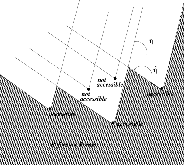
Figure 2: Picture of ${\cal P}_{\eta}\cap{\cal P}_{\tilde{\eta}}$.

We generalize propositions 3 of [3] without any assumptions on the values of $\lambda^{\prime}_{1},...,\lambda^{\prime}_{n}$.

Proposition 5

i) Let $\lambda_{k}$ be accessible w.r.t. some admissible $\eta$ and $\tilde{\eta}$. Then

$$\vec{\Psi}_{k}^{(k)}(\lambda,\eta)=\vec{\Psi}_{k}^{(k)}(\lambda,\tilde{\eta})~{}~{}\hbox{ and }~{}~{}\vec{\Psi}_{k}(\lambda,\eta)=\vec{\Psi}_{k}(\lambda,\tilde{\eta}),~{}~{}~{}\forall\lambda\in{\cal P}_{\eta}\cap{\cal P}_{\tilde{\eta}}$$

ii) Let $\eta$ and $\tilde{\eta}$ lie between two consecutive critical values: namely $\eta_{\nu+1}<\eta<\tilde{\eta}<\eta_{\nu}$. Then

$$C(\eta)=C(\tilde{\eta})$$

iii) Let again $\eta_{\nu+1}<\eta<\tilde{\eta}<\eta_{\nu}$. Then

$$\Psi^{*}(\lambda,\eta)=\Psi^{*}(\lambda,\tilde{\eta}),~{}~{}~{}\forall\lambda\in{\cal P}_{\eta}\cap{\cal P}_{\tilde{\eta}}.$$

whenever $\Psi^{*}$ is uniquely defined (namely, when $A_{1}$ has no negative integer eigenvalues).

Proof: See the Appendix. $\Box$

The above implies that the dependence on $\eta$ is discrete, namely it changes when a critical value is crossed. Thus, if $\eta_{\nu+1}<\eta<\eta_{\nu}$, we follow [3] and write

$$\Psi_{\nu}(\lambda):=\Psi(\lambda,\eta),~{}~{}~{}\Psi_{\nu}^{*}(\lambda):=\Psi^{*}(\lambda,\eta),~{}~{}~{}C_{\nu}=(c_{jk}^{(\nu)}):=C(\eta).$$

We now compute how $\Psi^{*}(\lambda,\eta)$ changes when $\eta$ changes, so generalizing proposition 4 of [3], without assumptions on $\lambda^{\prime}_{1},..,\lambda^{\prime}_{n}$.

Proposition 6

Suppose that $A_{1}$ has no negative integer eigenvalues, so that the $\Psi^{*}_{\nu}(\lambda)$’s exist, for $\nu\in\mathbb{Z}$. Let $\eta_{\nu+1}<\eta<\eta_{\nu}<\tilde{\eta}<\eta_{\nu-1}$. Then

$$\Psi^{*}_{\nu-1}(\lambda)=\Psi^{*}_{\nu}(\lambda)~{}W_{\nu},~{}~{}~{}~{}\forall\lambda\in{\cal P}_{\eta}\cap{\cal P}_{\tilde{\eta}},$$ (19)

where the invertible matrix $W_{\nu}=(W_{jk}^{(\nu)})$ is

$$W_{jk}^{(\nu)}=-\alpha_{k}c_{jk}^{(\nu)},~{}~{}\hbox{ for }j\succ k~{}\hbox{ such that }~{}\arg(\lambda_{j}-\lambda_{k})=\eta_{\nu}$$ (20)

$$W_{jj}^{(\nu)}=1,~{}~{}~{}j=1,\cdots,n;~{}~{}~{}~{}~{}~{}~{}~{}W_{jk}^{(\nu)}=0\hbox{ otherwise}.$$ (21)

where $\prec$ is the dominance relation w.r.t. $\eta$. In the same way,

$$\Psi^{*}_{\nu}(\lambda)=\Psi^{*}_{\nu-1}(\lambda)~{}W_{\nu}^{-1},~{}~{}~{}~{}\forall\lambda\in{\cal P}_{\eta}\cap{\cal P}_{\tilde{\eta}},$$

where $W_{\nu}^{-1}$ has zero entries except for

$$[W_{\nu}^{-1}]_{jj}=1,~{}~{}~{}j=1,\cdots,n,$$

$$[W_{\nu}^{-1}]_{jk}=-\beta_{k}c_{jk}^{(\nu-1)},~{}~{}\hbox{ for }j\succ k~{}\hbox{ s.t. }~{}\arg(\lambda_{j}-\lambda_{k})=\eta_{\nu}.$$

Note that $W_{jk}^{(\nu)}=-\alpha_{k}c_{jk}(\eta)$ for $\arg(\lambda_{j}-\lambda_{k})=\eta_{\nu}$ implies that $~{}j\succ k$, Proof: See the Appendix. $\Box$

In an angular interval $(\theta-2\pi,\theta]$, there are $m$ critical values, $m$ even. Let $\mu=m/2$. Let $\eta_{\nu+1}<\eta<\eta_{\nu}$ and introduce, as in [3], the matrices $C_{\nu}^{+}$ and $C_{\nu}^{-}$ such that

$$\Psi_{\nu+\mu}^{*}(\lambda)=\Psi_{\nu}^{*}(\lambda)C_{\nu}^{+},~{}~{}~{}~{}~{}~{}~{}\lambda\in{\cal P}_{\eta}\cap{\cal P}_{\eta-\pi}.$$ (22)

$$\Psi_{\nu+\mu}^{*}(\lambda)=\Psi_{\nu+m}^{*}(\lambda)C_{\nu}^{-},~{}~{}~{}~{}~{}~{}~{}\lambda\in{\cal P}_{\eta-\pi}\cap{\cal P}_{\eta-2\pi}$$ (23)

Immediately it follows that

$$C_{\nu}^{+}=(W_{\nu+\mu}\cdots W_{\nu+1})^{-1},~{}~{}~{}C_{\nu}^{-}=W_{\nu+m}\cdots W_{\nu+\mu+1}.$$ (24)

Note

Remark 6

${\cal P}_{\eta}\cap{\cal P}_{\eta-\pi}$ is the half plane to the left hand side of all lines whose positive parts are the cuts of direction $\eta$, while ${\cal P}_{\eta-\pi}\cap{\cal P}_{\eta-2\pi}$ is the half plane to the right hand side of all lines whose positive parts are the cuts of direction $\eta-2\pi$.

We restate remark 3.3 of [3] with no assumptions on $A_{1}$:

Lemma 4

Let $\Lambda^{\prime}:=\hbox{diag}(\lambda^{\prime}_{1},...,\lambda^{\prime}_{n})$, $\lambda^{\prime}_{k}\in\mathbb{C}$, $1\leq k\leq n$. Then

$$\Psi_{\nu+m}(\lambda)=\Psi_{\nu}(\lambda)e^{2\pi i\Lambda^{\prime}},$$

for any $\lambda$ in the universal covering of $\mathbb{C}\backslash\{\lambda_{1},...,\lambda_{n}\}$. Moreover

$$C_{\nu}=e^{2\pi i\Lambda^{\prime}}~{}C_{\nu+m}~{}e^{-2\pi i\Lambda^{\prime}},~{}~{}~{}~{}(\hbox{namely: }C(\eta)=e^{2\pi i\Lambda^{\prime}}~{}C(\eta-2\pi)~{}e^{-2\pi i\Lambda^{\prime}}).$$

Proof: See the Appendix. $\Box$

We generalize proposition 5 of [3], with no assumptions on diag$(A_{1})=(\lambda^{\prime}_{1},...,\lambda^{\prime}_{k})$.

Proposition 7

Let $\eta_{\nu+1}<\eta<\eta_{\nu}$, and let $c_{jk}^{(\nu)}~{}=c_{jk}(\eta)$. Consider the relation (22) and (23). The connection matrices $C_{\nu}^{+}$, $C_{\nu}^{-}$ are

$$[C_{\nu}^{+}]_{jk}=\left\{\matrix{-\beta_{k}~{}c_{jk}^{(\nu)}&=&e^{2\pi i\lambda^{\prime}_{k}}\alpha_{k}~{}c_{jk}^{(\nu)}&~{}~{}~{}\hbox{ for }j\prec k\cr\cr 1&&&~{}~{}~{}\hbox{ for }j=k\cr\cr 0&&&~{}~{}~{}\hbox{ for }j\succ k}\right.$$ (25)

$$[C_{\nu}^{-}]_{jk}=\left\{\matrix{0&&&~{}~{}~{}\hbox{ for }j\prec k\cr\cr 1&&&~{}~{}~{}\hbox{ for }j=k\cr\cr e^{-2\pi i\lambda^{\prime}_{j}}\beta_{k}~{}c_{jk}^{(\nu)}&=&-e^{2\pi i(\lambda^{\prime}_{k}-\lambda^{\prime}_{j})}\alpha_{k}~{}c_{jk}^{(\nu)}&~{}~{}~{}\hbox{ for }j\succ k}\right.$$ (26)

where $\alpha_{k}=e^{-2\pi i\lambda^{\prime}_{k}}-1$ if $\lambda^{\prime}_{k}\not\in\mathbb{Z}$, $\alpha_{k}=2\pi i$ if $\lambda^{\prime}_{k}\in\mathbb{Z}$, $\beta_{k}=e^{-2\pi i\lambda^{\prime}_{k}}\alpha_{k}$.

Proof: See the Appendix. $\Box$

The matrices $C_{\nu}^{+}$ and $C_{\nu}^{-}$ can be defined by formulae (25) and (26), independently of the fact that $A_{1}$ has no negative integer eigenvalues, namely independently of (22) and (23). The following corollary is a direct computation.

Corollary 5

Let the matrices $C_{\nu}^{+}$ and $C_{\nu}^{-}$ be defined by formulae (25) and (26). Then

$$\hbox{\rm Tr}(M_{k})=n-1+e^{-2\pi i\lambda^{\prime}_{k}}$$

$$\hbox{\rm Tr}(M_{j}M_{k})=\left\{\matrix{n-2+e^{-2\pi i\lambda^{\prime}_{j}}+e^{-2\pi i\lambda^{\prime}_{k}}-e^{-2\pi i\lambda^{\prime}_{j}}~{}[C_{\nu}^{+}]_{jk}[C_{\nu}^{-}]_{kj}&\hbox{ if }j\prec k,\cr\cr n-2+e^{-2\pi i\lambda^{\prime}_{j}}+e^{-2\pi i\lambda^{\prime}_{k}}-e^{-2\pi i\lambda^{\prime}_{k}}~{}[C_{\nu}^{-}]_{jk}[C_{\nu}^{+}]_{kj}&\hbox{ if }j\succ k.}\right.$$

If moreover $A_{1}$ has no integer eigenvalues, then

$$\hbox{\rm Tr}(M_{k}^{*})=\hbox{\rm Tr}(M_{k}),~{}~{}~{}~{}~{}~{}~{}~{}\hbox{\rm Tr}(M_{j}^{*}M_{k}^{*})=\hbox{\rm Tr}(M_{j}M_{k}).$$

5 Fundamental Solutions of (1) as Laplace Integrals

5.1 Fundamental solutions of (1) and Stokes Matrices

Definition 3

Stokes rays are the oriented rays from 0 to $\infty$ contained in the universal covering of $\mathbb{C}\backslash\{0\}$, defined by the condition

$$\Re(z(\lambda_{j}-\lambda_{k}))=0,~{}~{}~{}i\neq j,~{}~{}~{}1\leq i,j\leq n,~{}~{}~{}~{}~{}~{}~{}z\in\widetilde{\mathbb{C}\backslash\{0\}}.$$

Let $\eta\in\mathbb{R}$ be admissible, namely $\eta\neq\arg(\lambda_{i}-\lambda_{j})\hbox{ mod }2\pi$, for any $i\neq j$. We choose the Stokes rays

$$r_{jk}:=\Bigl{\{}z\in\mathbb{C}~{}|~{}z=\rho\exp\left\{i\left({3\pi\over 2}-\eta_{jk}\right)\right\},~{}\rho>0\Bigr{\}},~{}~{}~{}j\neq k,~{}~{}~{}1\leq j,k\leq n,$$

where

$$\eta_{jk}=\hbox{ determination of }\arg(\lambda_{j}-\lambda_{k})~{}~{}\hbox{ s.t. }\eta_{jk}\in(\eta-2\pi,\eta].$$

If follows that

$$\left\{\matrix{\Re(z(\lambda_{j}-\lambda_{k}))=0,&\hbox{for $z$ belonging to the ray,}\cr\Re(z(\lambda_{j}-\lambda_{k}))<0,&\hbox{for $z$ in the half plane to the right of $r_{jk}$.}}\right.$$

According to the definition, all the Stokes rays are characterized by

$$\arg z={3\pi\over 2}-\eta_{jk}~{}\hbox{ mod }2\pi.$$

Moreover, for any $(j,k)$ such that $\eta_{jk}<\eta<\eta_{jk}+\pi$ we have

$$\Re(z(\lambda_{j}-\lambda_{k}))<0~{}~{}~{}\hbox{\rm if }~{}~{}\arg z={3\pi\over 2}-\eta\hbox{ mod }2\pi.$$

This means that when we fix an admissible $\eta$ for system (2)-(3), we have

$$\Re(z(\lambda_{j}-\lambda_{k}))<0\hbox{ for }\arg z={3\pi\over 2}-\eta\hbox{ mod }2\pi~{}~{}~{}\Longleftrightarrow~{}~{}~{}j\prec k$$ (27)

Indeed, by (18), $j\prec k$ means that $-\pi+\eta<\eta_{jk}<\eta$. Relation (27) explains why we have called $\prec$ a dominance relation: in the half plane to the right of $r_{jk}$ the eigenvalue $\lambda_{k}$ is dominant w.r.t. $\lambda_{j}$, in the usual sense of asymptotic theory of ODE with singularities of the II kind. A Stokes ray is represented in figure 3.

Figure 3: Stokes’ ray $r_{jk}$, defined by $\arg z={3\pi\over 2}-\eta_{jk}$ mod $2\pi$. To the right of $r_{jk}$, $z={3\pi\over 2}-\eta$, with $\eta_{jk}<\eta<\eta_{jk}+\pi$, and $\Re(z(\lambda_{j}-\lambda_{k}))<0$.

In the same way as all the critical values $\eta_{\nu}$, $\nu\in\mathbb{Z}$, are obtained from $\eta_{jk}$ by adding multiples of $2\pi$, so all the Stokes rays are given by $\arg z=\tau_{\nu}$, where

$$\tau_{\nu}:={3\pi\over 2}-\eta_{\nu},$$

$$0\leq\tau_{0}<\tau_{1}<\cdots<\tau_{n}<2\pi;~{}~{}~{}~{}~{}\tau_{\nu+mh}=\tau_{n}+2\pi h,~{}~{}~{}h\in\mathbb{Z}.$$

Let us denote a sector in the universal covering $\widetilde{\mathbb{C}\backslash\{0\}}$ of $\mathbb{C}\backslash\{0\}$ in the following way

$$S(\alpha,\beta):=\{z\in\widetilde{\mathbb{C}\backslash\{0\}}~{}|~{}~{}~{}\alpha<\arg(z)<\beta\}.$$

The following result is known [13], [2]: in any sector

$${\cal S}_{\nu}:=S(\tau_{\nu}-\pi,\tau_{\nu+1}),~{}~{}~{}~{}~{}\nu\in\mathbb{Z},$$

equation (1) has a fundamental matrix solution

$$Y_{\nu}(z)=\hat{Y}_{\nu}(z)~{}e^{A_{0}z+\Lambda^{\prime}\ln z},~{}~{}~{}~{}~{}z\in{\cal S}_{\nu}$$ (28)

where $\Lambda^{\prime}=\hbox{ diag}(A_{1})$, and $\hat{Y}_{\nu}(z)$ is an invertible matrix, analytic in a neighbourhood of $\infty$, with asymptotic expansion

$$\hat{Y}_{\nu}(z)~{}\sim~{}I+{F_{1}\over z}+{F_{2}\over z^{2}}+\cdots~{}=I+\sum_{k=1}^{\infty}{F_{k}\over z^{k}},~{}~{}~{}~{}~{}~{}\hbox{ for }z\to\infty\hbox{ in }{\cal S}_{\nu}.$$ (29)

The sector ${\cal S}_{\nu}$ is the maximal sector where the asymptotic behavior holds, and $Y_{\nu}(z)$ is unique, namely it is uniquely determined by its asymptotic behavior. The $n\times n$ matrices $F_{k}$ are determined as rational functions of $A_{0}$ and $A_{1}$, by formal substitution into (1) (see [13], [2]).

Definition 4 (Stokes Matrices)

Given two fundamental matrices $Y_{\nu}$ and $Y_{\nu^{\prime}}$ as above, whose maximal sectors ${\cal S}_{\nu}$ and ${\cal S}_{\nu^{\prime}}$ intersect in such a way that no Stokes rays are contained in ${\cal S}_{\nu}\cap{\cal S}_{\nu^{\prime}}$, then the connection matrix $S$ such that $Y_{\nu^{\prime}}(z)=Y_{\nu}(z)S$, $z\in{\cal S}_{\nu}\cap{\cal S}_{\nu^{\prime}}$, is called a Stokes matrix.

Recall that in a sector $(\theta-2\pi,\theta]$ there are $m$ (even) critical values $\eta_{\nu}$, $\nu=\nu_{0},\nu_{0}+1,~{}...~{},\nu_{0}+m-1$, therefore in $[{3\pi\over 2}-\theta,{3\pi\over 2}-\theta+2\pi)$ there are $m$ Stokes rays with directions $\tau_{\nu}$, $\nu=\nu_{0},\nu_{0}+1,~{}...~{},\nu_{0}+m-1$. Again, let $\mu={m\over 2}$. Observe that $\eta_{\nu+\mu}=\eta_{\nu}-\pi$, therefore $\tau_{\nu+\mu}=\tau_{\nu}+\pi$. It follows that two matrices $Y_{\nu}$ and $Y_{\nu^{\prime}}$ satisfying the conditions above are precisely $Y_{\nu}(z)$ and $Y_{\nu+\mu}(z)$. Therefore (see figure 4):

Definition 4^′ (Stokes Matrices) For any $\nu\in\mathbb{Z}$ is defined the Stokes matrix $S_{\nu}$, which is the connection matrix such that

$$Y_{\nu+\mu}(z)=Y_{\nu}(z)S_{\nu},~{}~{}~{}~{}~{}z\in{\cal S}_{\nu}\cap{\cal S}_{\nu+\mu}=S(\tau_{\nu},\tau_{\nu+1}).$$

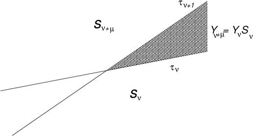
Figure 4: $Y_{\nu+\mu}(z)=Y_{\nu}(z)S_{\nu}$, $z\in{\cal S}_{\nu}\cap{\cal S}_{\nu+\mu}=S(\tau_{\nu},\tau_{\nu+1})$, $\nu\in\mathbb{Z}.$

Observe that $\Re(z(\lambda_{j}-\lambda_{k}))<0$ for $j\prec k$ when $z\in S(\tau_{\nu},\tau_{\nu+1})$, where the dominance relation is referred to a any $\eta\in(\eta_{\nu+1},\eta_{\nu})$. From the asymptotic behaviours of $Y_{\nu+\mu}(z)$ and $Y_{\nu}(z)$, it follows that $\delta_{jk}\sim e^{(\lambda_{j}-\lambda_{k})z}(S_{\nu})_{jk}$ and thus

$$(S_{\nu})_{jj}=1,~{}~{}~{}~{}~{}(S_{\nu})_{jk}=0~{}\hbox{ for }j\succ k.$$

Definition 5 (Stokes Factors)

The Stokes factors are the connection matrices $V_{\nu}$ such that

$$Y_{\nu-1}(z)=Y_{\nu}(z)V_{\nu},~{}~{}~{}~{}~{}z\in{\cal S}_{\nu-1}\cap{\cal S}_{\nu}=S(\tau_{\nu}-\pi,\tau_{\nu}).$$

It follows that $Y_{\nu+1}(z)=Y_{\nu+\mu}(z)V_{\nu+\mu}\cdots V_{\nu+1}$, (the r.h.s. is seen as the analytic continuation of the l.h.s.), and thus

$$S_{\nu}=\Bigl{(}V_{\nu+\mu}\cdots V_{\nu+1}\Bigr{)}^{-1}.$$ (30)

Observe that $\tau_{\nu}$ and $\tau_{\nu-\mu}=\tau_{\nu}-\pi=-\tau_{\nu}$ are not contained in $S(\tau_{\nu}-\pi,\tau_{\nu})$, while $\tau_{\nu-1},...,\tau_{\nu-\mu+1}$ are. It follows that $\Re(z(\lambda_{j}-\lambda_{k}))$ change sign in $S(\tau_{\nu}-\pi,\tau_{\nu})$ except for $(j,k)$ such that $\arg(\lambda_{j}-\lambda_{k})=\eta_{\nu}$, or $\eta_{\nu}-\pi$. Precisely, $\Re(z(\lambda_{j}-\lambda_{k}))<0$ if $\arg(\lambda_{j}-\lambda_{k})=\eta_{\nu}$, and $j\succ k$ with respect to $\eta\in(\eta_{\nu+1},\eta_{\nu})$. As above, we conclude that

$$(V_{\nu})_{jj}=1,$$

$$(V_{\nu})_{jk}=0~{}~{}~{}\forall~{}j\neq k,\hbox{ except possibly for }(j,k)\hbox{ s.t. }\left\{\matrix{\arg(\lambda_{j}-\lambda_{k})={3\pi\over 2}-\tau_{\nu}.\cr j\succ k\hbox{ w.r.t. }\eta\in(\eta_{\nu+1},\eta_{\nu}).}\right.$$

Remark 7

i) The monodromy of $Y_{\nu}(z)$ is completely described by the monodromy data $S_{\nu}$, $S_{\nu+\mu}$ and $\Lambda^{\prime}$, because the following holds

$$Y_{\nu}(ze^{2\pi i})=Y_{\nu}(z)e^{2\pi i\Lambda^{\prime}}(S_{\nu}S_{\nu+\mu})^{-1},~{}~{}~{}~{}~{}z\in{\cal S}_{\nu}.$$ (31)

For the above reason, $S_{\nu}$ and $S_{\nu+\mu}$ are a complete set of Stokes multiplies. Any other Stokes matrix can be expressed in terms of entries of $S_{\nu}$, $S_{\nu+\mu}$ and $\Lambda^{\prime}$.

ii) $S_{\nu}$ and $S_{\nu+\mu}$ are completely determined by $Y_{\nu}(z)$, $Y_{\nu+\mu}(z)$ and $\Lambda^{\prime}$, because

$$Y_{\nu+\mu}(z)=Y_{\nu}(z)S_{\nu},~{}~{}~{}~{}~{}z\in{\cal S}_{\nu}\cap{\cal S}_{\nu+\mu},$$ (32)

$$Y_{\nu}(ze^{-2\pi i})=Y_{\nu+\mu}(z)S_{\nu+\mu}e^{-2\pi i\Lambda^{\prime}},~{}~{}~{}~{}~{}z\in{\cal S}_{\nu+\mu}\cap{\cal S}_{\nu+m}.$$ (33)

iii) $Y_{\nu+m}(z)$ is determined by $Y_{\nu}(z)$ and $\Lambda^{\prime}$, because

$$Y_{\nu+m}(ze^{2\pi i})=Y_{\nu}(z)e^{2\pi i\Lambda^{\prime}},~{}~{}~{}~{}~{}z\in{\cal S}_{\nu}.$$ (34)

Remark 8

In [6], [7], [8], and oriented admissible line $l$, namely a line not containing Stokes rays, is introduced to define the analytic continuation of $Y_{\nu}$ and $Y_{\nu+\mu}$. The branch cut is taken to be the negative part of $l$. We can take $l=l(\eta)$ such that its positive part is the ray from 0 to $\infty$ with angle $\tau={3\pi\over 2}-\eta$.

Remark 9

If $A_{1}$ has some symmetries, then there may be a relation between $S_{\nu}$ and $S_{\nu+\mu}$. For example, in [6], [7] the case $A_{1}^{T}=-A_{1}$ is considered (where $T$ means transposition). This implies that

$$S_{\nu+\mu}^{T}=S_{\nu}^{-1}.$$

5.2 Solutions of (1) as Laplace Integrals

We consider a path $\gamma_{k}(\eta)$ which comes from infinity along the left side of the cut $L_{k}$ of direction $\eta$, encircles $\lambda_{k}$ with a small loop excluding all the other poles, and goes back to infinity along the right side of $L_{k}$ (where $L_{k}$ is oriented from $\lambda_{k}$ to $\infty$). See figure 5.

1) Case of $\lambda^{\prime}_{k}\not\in\mathbb{Z}$. We define

$$\overline{\underline{\left|\matrix{\cr~{}~{}\vec{Y}_{k}(z,\eta):={1\over 2\pi i}\int_{\gamma_{k}(\eta)}e^{z\lambda}~{}\vec{\Psi}_{k}(\lambda,\eta)~{}d\lambda~{}\equiv{1\over 2\pi i}\int_{\gamma_{k}(\eta)}e^{z\lambda}~{}\vec{\Psi}_{k}^{(k)}(\lambda,\eta)~{}d\lambda~{}~{}\cr\cr}\right|}}$$ (35)

Figure 5: The path $\gamma_{k}(\eta)$

Due to the fact that $\lambda_{k}$ is a regular singularity, the exponential ensures that the integral converges in the sector

$${\cal S}(\eta):=\left\{z\in\widetilde{\mathbb{C}\backslash\{0\}}~{}|~{}\Re(ze^{i\eta})<0\right\}~{}~{}~{}\Longrightarrow~{}~{}~{}{\pi\over 2}-\eta<\arg z<{3\pi\over 2}-\eta.$$ (36)

The asymptotic behaviour of (35) can be computed by expanding the integrand $\vec{\Psi}_{k}(\lambda)$ in series at $\lambda_{k}$ and then formally exchanging integration and series (see [5]). Namely, for any ${\cal N}>0$ integer,

$$\vec{Y}_{k}(z,\eta)={1\over 2\pi i}\int_{\gamma_{k}(\eta)}e^{z\lambda}~{}\left[\Gamma(\lambda^{\prime}_{k}+1)\vec{e}_{k}+\sum_{l\geq 1}\vec{b}_{l}^{~{}(k)}(\lambda-\lambda_{k})^{l}\right](\lambda-\lambda_{k})^{-\lambda^{\prime}_{k}-1}~{}d\lambda=(*)$$

Now write $\sum_{l\geq 1}=\sum_{l=1}^{\cal N}+\sum_{l>{\cal N}}$, and use the formula (see [5]):

$$\int_{\gamma_{k}(\eta)}(\lambda-\lambda_{k})^{-a}e^{z\lambda}d\lambda={z^{a-1}e^{\lambda_{k}z}\over\Gamma(a)}.$$

We obtain

$$(*)=\left(\vec{e}_{k}+\sum_{l=1}^{\cal N}{\vec{b}_{l}^{~{}(k)}\over\Gamma(\lambda^{\prime}_{k}+1-l)}~{}{1\over z^{l}}+{\cal R}(z)\right)~{}e^{\lambda_{k}z}z^{\lambda^{\prime}_{k}},$$ (37)

where ${\cal R}(z)$ is the integral of $\sum_{l>{\cal N}}$. It is standard computation to show that ${\cal R}(z)=O(z^{\cal N})$. Thus, formula (37) allows us to write the asymptotic expansion

$$\vec{Y}_{k}(z,\eta)~{}e^{-\lambda_{k}z}z^{-\lambda^{\prime}_{k}}\sim\vec{e}_{k}+\sum_{l=1}^{\infty}{\vec{b}_{l}^{~{}(k)}\over\Gamma(\lambda^{\prime}_{k}+1-l)}~{}{1\over z^{l}},~{}~{}~{}~{}~{}~{}~{}~{}z\to\infty,~{}~{}z\in{\cal S}(\eta).$$

Lemma 5

Assume $\lambda^{\prime}_{k}\not\in\mathbb{Z}$. Let $\eta\in(\eta_{\nu+1},\eta_{\nu})$, and $\tau_{\nu}:=3\pi/2-\eta_{\nu}$. Then, $\vec{Y}_{k}(z,\eta)$ defined by (35) is the $k$-th column of the unique fundamental solution of (1) identified by the asymptotic behavior (28), (29) in the sector

$${\cal S}_{\nu}=S(\tau_{\nu}-\pi,\tau_{\nu+1}).$$

Proof: If $\eta_{\nu+1}<\eta<\tilde{\eta}<\eta_{\nu}$, then $Y_{k}(z,\eta)=Y_{k}(z,\tilde{\eta})$. This defines the analytic continuation of (35) to

$$S(\tau_{\nu}-\pi,\tau_{\nu+1})=\bigcup_{\eta_{\nu+1}<\eta<\eta_{\nu}}{\cal S}(\eta),$$

with the required asymptotic behaviour. It remains to prove that $Y_{k}(z,\eta)$ is a vector solution of (1). This follows from integration by parts, as shown in the Introduction, since $\gamma_{k}(\eta)$ is such that $e^{\lambda z}(\lambda-A_{0})\vec{\Psi}_{k}(\lambda)\Bigl{|}_{\gamma_{k}}=0$. $\Box$

We write coefficients in (29) as

$$F_{k}=[~{}\vec{f}_{1}^{~{}(k)}~{}|~{}\cdots~{}|~{}\vec{f}_{n}^{~{}(k)}~{}]$$

Thus, we can write (6) for $\eta_{\nu+1}<\eta<\eta_{\nu}$ as

$$\overline{\underline{\left|\matrix{\cr~{}~{}\vec{\Psi}_{k}(\lambda,\eta)\equiv\vec{\Psi}_{k}^{(k)}(\lambda)=\sum_{l\geq 0}\Gamma(\lambda^{\prime}_{k}+1-l)~{}\vec{f}_{l}^{~{}(k)}~{}(\lambda-\lambda_{k})^{l-\lambda^{\prime}_{k}-1},~{}~{}~{}~{}~{}~{}~{}\vec{f}_{0}^{~{}(k)}=\vec{e}_{k}~{}~{}\cr\cr}\right|}}$$

2) Case of $\lambda^{\prime}_{k}=-1$. We define

$$\vec{Y}_{k}(z,\eta):=\int_{L_{k}}e^{z\lambda}~{}\vec{\Psi}_{k}(\lambda,\eta)~{}d\lambda~{}=-\int_{-L_{k}}e^{z\lambda}~{}\vec{\Psi}_{k}(\lambda,\eta)~{}d\lambda$$ (38)

along the cut $L_{k}$ from $\lambda_{k}$ to infinity. This is convergent in ${\cal S}(\eta)$ as before. Its asymptotic behaviour is obtained as before by expanding $\vec{\Psi}_{k}$ in the convergent series (7), and then exchanging integration and series, the result having meaning of asymptotic series. We obtain, by elementary integration:

$$Y_{k}(z,\eta)=\vec{e}_{k}\int_{-L_{k}}e^{z\lambda}d\lambda-\sum_{l\geq 1}\vec{b}_{l}^{~{}(k)}\int_{-L_{k}}(\lambda-\lambda_{k})^{l}e^{z\lambda}~{}d\lambda=$$

$$={e^{\lambda_{k}z}\over z}\left[\vec{e}_{k}+\sum_{l=1}^{\infty}(-1)^{l+1}~{}l!~{}~{}\vec{b}_{l}^{~{}(k)}{1\over z^{l}}\right].$$

where we have used the fact that

$$\int_{-L_{k}}(\lambda-\lambda_{k})^{l}e^{\lambda z}d\lambda={e^{\lambda_{k}z}\over z^{l+1}}\int_{+\infty e^{i\phi}}^{0}\xi^{l}e^{\xi}d\xi={e^{\lambda_{k}z}\over z^{l+1}}~{}l!~{}(-1)^{l},~{}~{}~{}~{}~{}{\pi\over 2}<\phi<{3\pi\over 2}.$$

The same proof of Lemma 5 yields the following

Lemma 6

Assume $\lambda^{\prime}_{k}=-1$. Let $\eta\in(\eta_{\nu+1},\eta_{\nu})$, and $\tau_{\nu}:=3\pi/2-\eta_{\nu}$. Then, $Y_{k}(z,\eta)$ defined by (38) is the $k$-th column of the unique fundamental solution of (1) identified by the asymptotic behavior (28), (29) in the sector

$${\cal S}_{\nu}=S(\tau_{\nu}-\pi,\tau_{\nu+1}).$$

By virtue of the lemma, we rewrite (7), for $\eta_{\nu+1}<\eta<\eta_{\nu}$, as follows

$$\overline{\underline{\left|\matrix{\cr~{}~{}\vec{\Psi}_{k}(\lambda,\eta)=-\vec{e}_{k}+\sum_{l\geq 1}{(-1)^{l+1}\over l!}\vec{f}_{l}^{~{}(k)}(\lambda-\lambda_{k})^{l}~{}~{}\cr\cr}\right|}}$$

Lemma 7

In case $\lambda^{\prime}_{k}=-1$, the solution (38) has also the representation

$$\overline{\underline{\left|\matrix{\cr~{}~{}\vec{Y}_{k}(z,\eta)=\int_{L_{k}}e^{z\lambda}~{}\vec{\Psi}_{k}(\lambda,\eta)~{}d\lambda~{}\equiv{1\over 2\pi i}\int_{\gamma_{k}(\eta)}\vec{\Psi}_{k}^{(k)}(\lambda)e^{z\lambda}~{}d\lambda~{}~{}\cr\cr}\right|}}$$ (39)

where $\gamma_{k}(\eta)$ is the same of (35).

Proof: Recall that $\vec{\Psi}_{k}^{(k)}=\vec{\Psi}_{k}(\lambda)\ln(\lambda-\lambda_{k})+\hbox{reg}(\lambda-\lambda_{k})$. Since

$$\int_{\gamma_{k}}\hbox{reg}(\lambda-\lambda_{k})~{}e^{z\lambda}~{}d\lambda=0$$

we have

$$\int_{\gamma_{k}(\eta)}\vec{\Psi}_{k}^{(k)}(\lambda)~{}e^{z\lambda}~{}d\lambda=\int_{\gamma_{k}(\eta)}\vec{\Psi}_{k}(\lambda)\ln(\lambda-\lambda_{k})~{}e^{z\lambda}~{}d\lambda$$

Indicate with $L_{k}^{L}$ and $L_{k}^{R}$ the left and right sides of $L_{k}$ (oriented from $\lambda_{k}$ to $\infty$), and with $(\lambda-\lambda_{k})_{R/L}$ the branch of $(\lambda-\lambda_{k})$ to the right/left of $L_{k}$. Then

$$\int_{\gamma_{k}(\eta)}=\int_{-L_{k}^{L}}~{}+\int_{L_{k}^{R}}~{}=\int_{L_{k}^{R}}~{}-\int_{L_{k}^{L}}~{}=(*)$$

Moreover

$$(\lambda-\lambda_{k})_{L}=e^{-2\pi i}(\lambda-\lambda_{k})_{R},~{}~{}~{}\hbox{ where }\arg((\lambda-\lambda_{k})_{R})=\eta.$$

Therefore

$$(*)=\int_{L_{k}^{R}}\vec{\Psi}_{k}(\lambda)\ln(\lambda-\lambda_{k})_{R}~{}e^{z\lambda}~{}d\lambda+\left\{2\pi i\int_{L_{k}}\vec{\Psi}_{k}(\lambda)~{}e^{z\lambda}~{}d\lambda-\int_{L_{k}^{R}}\vec{\Psi}_{k}(\lambda)\ln(\lambda-\lambda_{k})_{R}~{}e^{z\lambda}~{}d\lambda\right\}$$

$$\equiv 2\pi i\int_{L_{k}}\vec{\Psi}_{k}(\lambda)~{}e^{z\lambda}~{}d\lambda.$$

$\Box$

3) Case of $\lambda^{\prime}_{k}\in\mathbb{N}$. Define the convergent in ${\cal S}(\eta)$ integral

$$\overline{\underline{\left|\matrix{\cr~{}~{}\vec{Y}_{k}(z,\eta):={1\over 2\pi i}\int_{\gamma_{k}(\eta)}e^{z\lambda}~{}\vec{\Psi}_{k}^{(k)}(\lambda,\eta)~{}d\lambda~{}~{}\cr\cr}\right|}}$$ (40)

where

$$\vec{\Psi}^{(k)}_{k}(\lambda)=\vec{\Psi}_{k}(\lambda)\ln(\lambda-\lambda_{k})+{P_{N_{k}}^{(k)}(\lambda)\over(\lambda-\lambda_{k})^{N_{k}+1}}+\hbox{reg}(\lambda-\lambda_{k}),$$

$$\vec{\Psi}_{k}=\sum_{l\geq 0}{\vec{d}_{l}}^{~{}(k)}(\lambda-\lambda_{k})^{l},~{}~{}~{}P_{N_{k}}^{(k)}=N_{k}!~{}\vec{e}_{k}+\sum_{l=0}^{N_{k}}\vec{b}_{l}^{~{}(k)}(\lambda-\lambda_{k})^{l},$$

As before, we prove that

$${1\over 2\pi i}\int_{\gamma_{k}(\eta)}e^{z\lambda}\vec{\Psi}_{k}(\lambda)\ln(\lambda-\lambda_{k})d\lambda=\int_{L_{k}}e^{z\lambda}\vec{\Psi}_{k}(\lambda)d\lambda$$

$$=\sum_{l=0}^{\infty}(-1)^{l+1}~{}l!~{}d_{l}^{~{}(k)}~{}{1\over z^{l+1}}~{}e^{z\lambda_{k}}.$$

where ”$=$” means asymptotic for $z\to\infty$. On the other hand, by Cauchy theorem,

$${1\over 2\pi i}\int_{\gamma_{k}(\eta)}e^{z\lambda}{P^{(k)}(\lambda)\over(\lambda-\lambda_{k})^{N_{k}+1}}={1\over N_{k}!}{d^{N_{k}}\over d\lambda^{N_{k}}}\left.\left(P^{(k)}(\lambda)e^{z\lambda}\right)\right|_{\lambda=\lambda_{k}}$$

$$=e^{\lambda_{k}z}~{}\sum_{q=0}^{N_{k}}{\vec{b}_{N_{k}-q}^{~{}(k)}\over q!}~{}z^{q}=\left[\vec{e}_{k}+\cdots+{\vec{b}_{N_{k}}^{(k)}\over z^{N_{k}}}\right]z^{N_{k}}e^{\lambda_{k}z},~{}~{}~{}~{}~{}\vec{b}_{0}^{~{}(k)}=N_{k}!~{}\vec{e}_{k}.$$

We conclude that $\vec{Y}_{k}(z,\eta)$ has the correct asymptotics. The same proof of Lemma 5 yields the following

Lemma 8

Assume $\lambda^{\prime}_{k}\in\mathbb{N}$. Let $\eta\in(\eta_{\nu+1},\eta_{\nu})$, and $\tau_{\nu}:=3\pi/2-\eta_{\nu}$. Then, $\vec{Y}_{k}(z,\eta)$ defined by (40) is the $k$-th column of the unique fundamental solution of (1) identified by the asymptotic behavior (28), (29) in the sector

$${\cal S}_{\nu}=S(\tau_{\nu}-\pi,\tau_{\nu+1}).$$

Accordingly, we rewrite for $\eta_{\nu+1}<\eta<\eta_{\nu}$:

$$\overline{\underline{\left|\matrix{\cr~{}~{}\vec{\Psi}_{k}^{(k)}(\lambda,\eta)=\sum_{l=0}^{N_{k}}(N_{k}-l)!~{}\vec{f}_{l}^{~{}(k)}~{}u^{l-N_{k}-1}+\left[\sum_{l=0}^{\infty}{(-1)^{l+1}~{}\vec{f}_{N_{k}+l+1}^{~{}(k)}\over l!}~{}u^{l}\right]\ln(u)+\hbox{reg}(u)~{}~{}\cr\cr}\right|}}$$

where $u:=\lambda-\lambda_{k}$.

4) case of $\lambda^{\prime}_{k}=N_{k}\in-\mathbb{N}-2$. We define

$$\overline{\underline{\left|\matrix{\cr~{}~{}\vec{Y}_{k}(z,\eta):=\int_{L_{k}}e^{z\lambda}\vec{\Psi}_{k}(\lambda)d\lambda~{}~{}\cr\cr}\right|}}$$ (41)

The asymptotic behaviour of the above is readily computed:

$$\int_{L_{k}}e^{z\lambda}\vec{\Psi}_{k}(\lambda)d\lambda=\int_{L_{k}}e^{z\lambda}\sum_{l\geq 0}\vec{b}_{l}^{(k)}(\lambda-\lambda_{k})^{l-N_{k}-1}d\lambda$$

$$=e^{\lambda_{k}z}(-1)^{N_{k}}\sum_{l\geq 0}{(-1)^{l}(l-N_{k}-1)!~{}\vec{b}_{l}^{(k)}\over z^{l-N_{k}}}$$

$$=\left[\vec{e}_{k}+(-1)^{N_{k}}\sum_{l\geq 1}(-1)^{l}(l-N_{k}-1)!~{}\vec{b}_{l}^{(k)}~{}{1\over z^{l}}\right]z^{N_{k}}e^{\lambda_{k}z}.$$

where we have used the normalization $\vec{b}_{0}^{(k)}=(-1)^{N_{k}}\vec{e}_{k}/(-N_{k}-1)!$. We conclude that $\vec{Y}_{k}(z,\eta)$ has the correct asymptotics. The same proof of Lemma 5 yields the following

Lemma 9

Assume $\lambda^{\prime}_{k}=N_{k}\in-\mathbb{N}-2$. Let $\eta\in(\eta_{\nu+1},\eta_{\nu})$, and $\tau_{\nu}:=3\pi/2-\eta_{\nu}$. Then, $\vec{Y}_{k}(z,\eta)$ defined by (41) is the $k$-th column of the unique fundamental solution of (1) identified by the asymptotic behaviour (28), (29) in the sector

$${\cal S}_{\nu}=S(\tau_{\nu}-\pi,\tau_{\nu+1}).$$

Accordingly:

$$\overline{\underline{\left|\matrix{\cr~{}~{}\vec{\Psi}_{k}(\lambda)=\sum_{l\geq 0}{(-1)^{l-N_{k}}\over(l-N_{k}-1)!}~{}\vec{f}_{l}^{(k)}~{}(\lambda-\lambda_{k})^{l-N_{k}-1}~{}~{}\cr\cr}\right|}}$$

Also in this case we have

$${1\over 2\pi i}\int_{\gamma_{k}(\eta)}e^{z\lambda}\vec{\Psi}_{k}(\lambda)\ln(\lambda-\lambda_{k})d\lambda=\int_{L_{k}}e^{z\lambda}\vec{\Psi}_{k}(\lambda)d\lambda$$

Therefore, when the singular solution $\vec{\Psi}_{k}(\lambda)\ln(\lambda-\lambda_{k})+\hbox{reg}(\lambda-\lambda_{k})$ exists, we have

$$\overline{\underline{\left|\matrix{\cr~{}~{}\vec{Y}_{k}(z,\eta)=\int_{\gamma_{k}(\eta)}e^{z\lambda}\Bigl{(}\vec{\Psi}_{k}(\lambda)\ln(\lambda-\lambda_{k})+\hbox{reg}(\lambda-\lambda_{k})\Bigr{)}d\lambda.~{}~{}\cr\cr}\right|}}$$

Proposition 8

The following are the fundamental matrix solutions of (1) uniquely identified by the asymptotic behaviour (28), (29) in ${\cal S}_{\nu}$, $\nu\in\mathbb{Z}$:

$$Y_{\nu}(z)=\left[~{}\vec{Y}_{1}(z,\eta)~{}|~{}\cdots~{}|~{}\vec{Y}_{n}(z,\eta)~{}\right]$$

$$\vec{Y}_{k}(z,\eta)={1\over 2\pi i}\int_{\gamma_{k}(\eta)}e^{z\lambda}~{}\vec{\Psi}_{k}^{(sing)}(\lambda,\eta)~{}d\lambda,~{}~{}~{}1\leq k\leq n,~{}~{}~{}~{}\eta_{\nu}<\eta<\eta_{\nu+1},$$ (42)

where $\vec{\Psi}_{k}^{(sing)}$ is defined in (13). In case it happens that $\vec{\Psi}^{(sing)}=0$, $\lambda^{\prime}_{k}\in-\mathbb{N}-2$, then (42) is replaced by (41).

Proof: The above is a consequence of the preceding discussion. Linear independence of the columns of $Y_{\nu}(z)$ follows from the independence of the first term of the asymptotic behaviour of each column. Uniqueness follows from the maximality of the sector. $\Box$

Lemma 10

If $A_{1}$ has no negative integer eigenvalues, then, $\vec{\Psi}_{k}^{(sing)}$ in the integral (42) can be replaced by $\vec{\Psi}_{k}^{*}$ . Namely:

$$\vec{Y}_{k}(z,\eta)={1\over 2\pi i}\int_{\gamma_{k}(\eta)}e^{z\lambda}~{}\vec{\Psi}_{k}^{*}(\lambda,\eta)~{}d\lambda,~{}~{}~{}1\leq k\leq n,~{}~{}~{}~{}\eta_{\nu}<\eta<\eta_{\nu+1}.$$

Proof: Recall that if $A_{1}$ has no negative integer eigenvalues, then $\vec{\Psi}^{(sing)}\neq 0$ also for $\lambda^{\prime}_{k}\in-\mathbb{N}-2$. Since $\vec{\Psi}_{k}^{(sing)}-\vec{\Psi}_{k}^{*}=\hbox{reg}(\lambda-\lambda_{k})$, we have

$$\int_{\gamma_{k}(\eta)}\left(\vec{\Psi}_{k}^{(sing)}(\lambda)-\vec{\Psi}_{k}^{*}(\lambda)\right)e^{z\lambda}d\lambda=0.$$

$\Box$

6 Stokes Factors and Matrices in terms of $C$ - Main Theorem (Th. 1)

In this section we state the main result of the paper, which is Theorem 1 and Corollary 6.

Consider as in [3] a new path of integration $\gamma(\eta)$ homotopic to the product $\gamma_{k_{n}}(\eta)\cdots\gamma_{k_{1}}(\eta)$, $k_{1}\prec k_{2}\prec...\prec k_{n}$, namely a path coming from $\infty$ in direction $\eta$ to the left of all the poles $\lambda_{1},...,\lambda_{n}$, encircling all the poles, and going back to $\infty$ in direction $\eta$ to the right of all the poles. The following Proposition is the generalization of Theorem $2^{\prime}$ of [3] when no assumptions are made on diag$(A_{1})$.

Proposition 9

If $A_{1}$ has no negative integer eigenvalues the fundamental matrix of Proposition 8 is

$$Y_{\nu}(z)={1\over 2\pi i}\int_{\gamma(\eta)}~{}e^{z\lambda}~{}\Psi^{*}(\lambda,\eta)~{}d\lambda,~{}~{}~{}~{}~{}\eta_{\nu+1}<\eta<\eta_{\nu}.$$

and

$$Y_{\nu-1}(z)=Y_{\nu}(z)W_{\nu},~{}~{}~{}~{}~{}z\in{\cal S}_{\nu-1}\cap{\cal S}_{\nu}=S(\tau_{\nu}-\pi,\tau_{\nu}).$$

where the $W_{\nu}$’s are given in Proposition 6. Therefore, the Stokes factors are

$$V_{\nu}=W_{\nu}$$

Moreover,

$$S_{\nu}=C_{\nu}^{+},~{}~{}~{}~{}~{}S_{\nu+m}^{-1}=C_{\nu}^{-}.$$

Proof: The first statement is easy. Indeed $\Psi_{k}^{*}(\lambda)=\hbox{reg}(\lambda-\lambda_{j})$ for any $j\neq k$ implies

$$\int_{\gamma_{k}(\eta)}~{}e^{z\lambda}~{}\vec{\Psi}_{k}^{*}(\lambda,\eta)~{}d\lambda=\int_{\gamma(\eta)}~{}e^{z\lambda}~{}\vec{\Psi}_{k}^{*}(\lambda,\eta)~{}d\lambda$$

Then,we consider $\eta_{\nu+1}<\eta<\eta_{\nu}<\tilde{\eta}<\eta_{\nu-1}$ and

$$2\pi iY_{\nu-1}(z)=\int_{\gamma(\tilde{\eta})}~{}e^{z\lambda}~{}\Psi^{*}(\lambda,\tilde{\eta})~{}d\lambda=(*)$$

We can define the analytic continuation of $\Psi^{*}(\lambda,\tilde{\eta})$ along $\gamma(\eta)$ as follows. We consider on $\gamma(\tilde{\eta})$ a reference point $\lambda_{0}$ w.r.t. both $\tilde{\eta}$ and $\eta$, and deform $\gamma(\tilde{\eta})$ by keeping $\lambda_{0}$ fixed, until we obtain $\gamma(\eta)$. See fifure 6. Since $\lambda_{0}$ is a reference point, $\Psi^{*}(\lambda_{0},\tilde{\eta})=\Psi^{*}(\lambda_{0},\eta)$. Thus the analytic continuation of $\Psi^{*}(\lambda,\tilde{\eta})$ along $\gamma(\eta)$ is $\Psi^{*}(\lambda,\eta)W_{\nu}$. Consequently

$$(*)=\int_{\gamma(\eta)}~{}e^{z\lambda}~{}\left(\Psi^{*}(\lambda,\eta)W_{\nu}\right)~{}d\lambda=\left(\int_{\gamma(\eta)}~{}e^{z\lambda}~{}\Psi^{*}(\lambda,\eta)~{}d\lambda\right)~{}W_{\nu}~{}\equiv 2\pi iY_{\nu}(z)W_{\nu}.$$

The last statement follows from (24) and (30). $\Box$

Figure 6: The paths $\gamma(\eta)$ and $\gamma(\tilde{\eta})$.

We are going to prove that the statement of the above Proposition holds also for any $A_{1}$, without assumptions. This result is the following

Theorem 1

Let $A_{1}$ be any $n\times n$ matrix, with no assumptions. The Stokes multipliers and matrices of system (1) are given in terms of the connection coefficients $c_{jk}^{(\nu)}$ of system (2) according to the formulae

$$\overline{\underline{\left|\matrix{\cr~{}~{}V_{\nu}=W_{\nu},~{}~{}~{}~{}~{}~{}S_{\nu}=C_{\nu}^{+},~{}~{}~{}~{}~{}S_{\nu+m}^{-1}=C_{\nu}^{-},~{}~{}~{}~{}~{}\forall\nu\in\mathbb{Z}~{}~{}\cr\cr}\right|}}$$

where $W_{\nu}$ is defined by formulae (20), (21), and $C_{\nu}^{+}$ and $C_{\nu}^{-}$ are defined by formulae (25) and (26).

Remark: Here formulae (20), (21), (25) and (26) are taken as the definitions of $W_{\nu}$, $C_{\nu}^{+}$ and $C_{\nu}^{-}$, independently of the existence of $\Psi^{*}(\lambda)$.

Corollary 6

Let $A_{1}$ be any $n\times n$ matrix, with no assumptions. The following equalities hold for the monodromy matrices of $\Psi(\lambda)$ of system (2)-(3), defined in (14):

$$\overline{\underline{\left|\matrix{\cr~{}~{}\hbox{\rm Tr}(M_{k})=n-1+e^{-2\pi i\lambda^{\prime}_{k}}~{}~{}\cr\cr}\right|}}$$

$$\overline{\underline{\left|\matrix{\cr~{}~{}\hbox{\rm Tr}(M_{j}M_{k})=\left\{\matrix{n-2+e^{-2\pi i\lambda^{\prime}_{j}}+e^{-2\pi i\lambda^{\prime}_{k}}-e^{-2\pi i\lambda^{\prime}_{j}}~{}[S_{\nu}]_{jk}[S_{\nu+m}^{-1}]_{kj}&\hbox{ if }j\prec k,\cr\cr n-2+e^{-2\pi i\lambda^{\prime}_{j}}+e^{-2\pi i\lambda^{\prime}_{k}}-e^{-2\pi i\lambda^{\prime}_{k}}~{}[S_{\nu+m}^{-1}]_{jk}[S_{\nu}]_{kj}&\hbox{ if }j\succ k.}\right.~{}~{}\cr\cr}\right|}}$$

The corollary above is a restatement of Corollary 5. We prove Theorem 1 in a few steps.

7 Proof of Theorem 1

We define

$${}_{\gamma}Y(z):=z^{-\gamma}Y(z),$$

which yields a gauge transformation of the linear systems (1):

$$\frac{d}{dz}~{}({}_{\gamma}Y)=\left(A_{0}+{A_{1}-\gamma\over z}\right)~{}{}_{\gamma}Y$$ (43)

The fundamental solutions ${}_{\gamma}Y_{\nu}(z)=z^{-\gamma}Y_{\nu}(z)$, have the same Stokes multiplier and Stokes matrices than $Y_{\nu}(z)$, and their columns are obtained as Laplace transforms of solutions of

$$(A_{0}-\lambda){d\over d\lambda}(~{}{}_{\gamma}\Psi)=(A_{1}-\gamma+I)~{}{}_{\gamma}\Psi.$$ (44)

If $A_{1}$ has diagonal entries $\lambda^{\prime}_{1},...,\lambda^{\prime}_{n}$, some of which may be integers, then we can always find a sufficiently small $\gamma_{0}>0$ such that, for any $0<\gamma<\gamma_{0}$, $A_{1}-\gamma$ has diagonal entries $\lambda^{\prime}_{1}-\gamma,...,\lambda^{\prime}_{n}-\gamma$ which are not integers, and moreover has no integer eigenvalues, so that $\Psi^{*}$ exists. In the following, we assume that $\gamma$ has this property.

For system (2), the matrix $C_{\nu}=(c_{jk}^{(\nu)})$ is defined by (4). Consequently, the matrices $C_{\nu}^{+}$ and $C_{\nu}^{-}$ are always defined by the formulae of Proposition 7, independently of the existence of $\Psi^{*}$ and formulae (22) and (23). On the other hand, for system (44) the matrices $C_{\nu}^{+}$ and $C_{\nu}^{-}$ (which depend on $\gamma$, so we write $C_{\nu}^{+}[\gamma]$ and $C_{\nu}^{-}[\gamma]$), are well defined by formulae (22) and (23). According to Proposition 7, their entries are again given in terms of $\gamma$-dependent connection coefficients $c_{jk}^{(\nu)}=c_{jk}^{(\nu)}[\gamma]$’s. The latter are defined by the first equality of (4) applied to the solutions $~{}{}_{\gamma}\vec{\Psi}_{k}$, namely:

$${}_{\gamma}\vec{\Psi}_{k}(\lambda)=~{}{}_{\gamma}\vec{\Psi}_{j}(\lambda)~{}c_{jk}^{(\nu)}[\gamma]~{}+\hbox{reg}(\lambda-\lambda_{j})$$ (45)

The following Proposition is the key step to prove Theorem 1

Proposition 10

Let $\gamma_{0}>0$ be small enough such that the diagonal part of $A_{1}-\gamma I$ has no integer entries and $A_{1}$ has no integer eigenvalues for any $0<\gamma<\gamma_{0}$. Let $\eta_{\nu+1}<\eta<\eta_{\nu}$ be fixed. Let $c_{jk}^{(\nu)}$ be the corresponding connection coefficients of system (2), defined by (4), and $c_{jk}^{(\nu)}[\gamma]$ be the connection coefficients of (44), defined by (45). Finally, let

$$\alpha_{k}=\left\{\matrix{e^{-2\pi i\lambda^{\prime}_{k}}-1,&\lambda^{\prime}_{k}\not\in\mathbb{Z}\cr\cr 2\pi i,&\lambda^{\prime}_{k}\in\mathbb{Z}}\right.;~{}~{}~{}~{}~{}~{}~{}~{}\alpha_{k}[\gamma]=e^{-2\pi i(\lambda^{\prime}_{k}-\gamma)}-1$$

Then, the following equalities hold

$$\alpha_{k}c_{jk}^{(\nu)}=e^{-2\pi i\gamma}\alpha_{k}[\gamma]~{}c_{jk}^{(\nu)}[\gamma],~{}~{}~{}\hbox{ if }k\succ j$$

$$\alpha_{k}c_{jk}^{(\nu)}=\alpha_{k}[\gamma]~{}c_{jk}^{(\nu)}[\gamma],~{}~{}~{}~{}~{}~{}~{}~{}~{}~{}~{}\hbox{ if }k\prec j$$

where the partial ordering $\prec$ refers to $\eta$.

Corollary 7

Let $\gamma$ be as in Proposition 10. Let $C_{\nu}^{+}[\gamma]$ and $C_{\nu}^{-}[\gamma]$ be the connection matrices defined in (22) and (23) for system (44). Let $C_{\nu}^{+}$ and $C_{\nu}^{-}$ be the matrices for system (2) defined by (25) and (26), where the $c_{jk}^{(\nu)}$ are defined by (4). Then

$$C_{\nu}^{+}=C_{\nu}^{+}[\gamma],~{}~{}~{}~{}~{}C_{\nu}^{-}=C_{\nu}^{-}[\gamma],~{}~{}~{}~{}~{}~{}~{}~{}\forall\nu\in\mathbb{Z}.$$

Also, let $W_{\nu}$ be defined by (20) and (21) for system (2), and $W_{\nu}[\gamma]$ be the matrix defined by (19) for system (44). Then

$$W_{\nu}=W_{\nu}[\gamma],~{}~{}~{}~{}~{}~{}~{}~{}\forall\nu\in\mathbb{Z}.$$

Proof of Corollary 7: It is enough to compare the formulae of Proposition 10 with those of Propositions 7 and 6. $\Box$

Before proving Proposition 10, we give the proof of Theorem 1.

Proof of Theorem 1: The $S_{\nu}$’s are unchanged by the gauge ${}_{\gamma}Y(z)=z^{-\gamma}Y(z)$. Moreover, Proposition 9 applies to the system (44), therefore

$$S_{\nu}=C_{\nu}^{+}[\gamma],~{}~{}~{}~{}~{}S_{\nu+m}^{-1}=C_{\nu}^{-}[\gamma],~{}~{}~{}~{}~{}V_{\nu}=W_{\nu}[\gamma].$$

Thus, Corollary 7 implies Theorem 1. $\Box$.

7.1 Proof of Proposition 10, by steps

The idea is the same of the proof of Lemma $2^{\prime}$ in [3], but with considerably more technical efforts, do to the fact that, unlike [3], we do not make any assumption on the diagonal entries of $A_{1}$. We need a few steps, which are Propositions 11 and 12 , and Lemmas 11, 12 below. First, we introduce the $q$-primitives of vector solutions of system (3).

– For $\lambda^{\prime}_{k}\in\mathbb{C}\backslash\mathbb{N}$ we have solutions

$$\vec{\Psi}_{k}(\lambda)=\sum_{l=0}^{\infty}\Gamma(\lambda^{\prime}_{k}+1-l)\vec{f}_{l}^{~{}(k)}~{}(\lambda-\lambda_{k})^{l-\lambda^{\prime}_{k}-1},~{}~{}~{}~{}~{}\lambda^{\prime}_{k}\not\in\mathbb{Z}$$

and

$$\vec{\Psi}_{k}(\lambda)=\sum_{l=0}^{\infty}{(-1)^{l-N_{k}}\over(l-N_{k}-1)!}~{}\vec{f}_{l}^{~{}(k)}~{}(\lambda-\lambda_{k})^{l-N_{k}-1},~{}~{}~{}~{}~{}\lambda^{\prime}_{k}=N_{k}\in\mathbb{Z}_{-}.$$

We define the $q$ primitive of $\vec{\Psi}_{k}$. This is the function $(\vec{\Psi}_{k})^{[-q]}(\lambda)$, $q\in\mathbb{N}$, given by analytic continuation of the series obtained by $q$-fold term wise integration of the corresponding term in $\vec{\Psi}_{k}(\lambda)$. Namely:

$$(\vec{\Psi}_{k})^{[-q]}(\lambda):=(-1)^{q}~{}\sum_{l=q}^{\infty}\Gamma(\lambda^{\prime}_{k}+1-l)\vec{f}_{l-q}^{~{}(k)}~{}(\lambda-\lambda_{k})^{l-\lambda^{\prime}_{k}-1},~{}~{}~{}~{}~{}\lambda^{\prime}_{k}\not\in\mathbb{Z}$$ (46)

$$(\vec{\Psi}_{k})^{[-q]}(\lambda):=(-1)^{q}\sum_{l=q}^{\infty}{(-1)^{l-N_{k}}\over(l-N_{k}-1)!}~{}\vec{f}_{l-q}^{~{}(k)}~{}(\lambda-\lambda_{k})^{l-N_{k}-1},~{}~{}~{}~{}~{}\lambda^{\prime}_{k}=N_{k}\leq-1.$$ (47)

They above converge in a neighbourhood of $\lambda_{k}$, contained in ${\cal P}_{\eta}$, where $\vec{\Psi}_{k}$ has convergent series. Indeed, if $\lambda_{0}\neq\lambda_{k}$ is in the neighbourhood, then

$$\int_{\lambda_{0}}^{\lambda}ds_{1}\int_{\lambda_{0}}^{s_{1}}ds_{2}\cdots\int_{\lambda_{0}}^{s_{q-1}}ds_{q}\vec{\Psi}_{k}(s_{q})=(\vec{\Psi}_{k})^{[-q]}(\lambda)-Q_{q-1}(\lambda-\lambda_{0})$$ (48)

where

$$Q_{q-1}(\lambda-\lambda_{0})=(\vec{\Psi}_{k})^{[-q]}(\lambda_{0})+(\vec{\Psi}_{k})^{[1-q]}(\lambda_{0})(\lambda-\lambda_{0})+~{}~{}~{}~{}~{}~{}~{}~{}~{}~{}~{}~{}~{}~{}~{}~{}~{}~{}~{}$$

$$~{}~{}~{}~{}~{}~{}~{}~{}~{}~{}~{}~{}~{}~{}~{}~{}~{}~{}~{}~{}~{}~{}~{}~{}+{(\vec{\Psi}_{k})^{[2-q]}(\lambda_{0})\over 2!}(\lambda-\lambda_{0})^{2}+\cdots+{(\vec{\Psi}_{k})^{[-1]}(\lambda_{0})\over(q-1)!}(\lambda-\lambda_{0})^{q-1}$$

is a polynomial in $(\lambda-\lambda_{0})$ of degree $q-1$. The path of integration is any in ${\cal P}_{\eta}$, such that $|\lambda-\lambda_{0}|$ is small enough for the series of $\vec{\Psi}_{k}$ to converge. In particular, for $\Re\lambda^{\prime}_{k}<0$,

$$(\vec{\Psi}_{k})^{[-q]}(\lambda)=\int_{\lambda_{k}}^{\lambda}ds_{1}\int_{\lambda_{k}}^{s_{1}}ds_{2}\cdots\int_{\lambda_{k}}^{s_{q-1}}ds_{q}\vec{\Psi}_{k}(s_{q})$$

Once $(\vec{\Psi}_{k})^{[-q]}(\lambda)$ is defined by the convergent series, then it is analytically continued to ${\cal P}_{\eta}$.

– For $\lambda^{\prime}_{k}=N_{k}\in\mathbb{N}$ integer, consider the solution

$$\vec{\Psi}_{k}^{(k)}(\lambda)=\vec{\Psi}_{k}(\lambda)\ln(\lambda-\lambda_{k})+{P_{N_{k}}^{(k)}(\lambda)\over(\lambda-\lambda_{k})^{N_{k}+1}}+\hbox{reg}(\lambda-\lambda_{k})$$

$$P_{N_{k}}^{(k)}(\lambda)=\sum_{l=0}^{N_{k}}(N_{k}-l)!~{}\vec{f}_{l}^{~{}(k)}~{}(\lambda-\lambda_{k})^{l}$$

$$\vec{\Psi}_{k}(\lambda)=\sum_{l=0}^{\infty}{(-1)^{l+1}\over l!}~{}\vec{f}_{N_{k}+l+1}^{~{}(k)}~{}(\lambda-\lambda_{k})^{l}$$

The series is convergent in a neighbourhood of $\lambda_{k}$ contained in ${\cal P}_{\eta}$. Let $\lambda_{0}$ belong to the neighbourhood. Let $q\geq 0$ integer, and compute $q$ times the integral of $\vec{\Psi}_{k}^{(k)}(\lambda)$. Due to convergence of the series, we can take integration term by term. We obtain:

i) For $q\leq N_{k}$:

$$\int_{\lambda_{0}}^{\lambda}ds_{1}\int_{\lambda_{0}}^{s_{1}}ds_{2}\cdots\int_{\lambda_{0}}^{s_{q-1}}ds_{q}\vec{\Psi}_{k}^{(k)}(s_{q})=$$

$$=\sum_{l=0}^{\infty}{(-1)^{l+1-q}\over l!}~{}\vec{f}_{N_{k}+1+l-q}^{~{}(k)}~{}(\lambda-\lambda_{k})^{l}~{}\ln(\lambda-\lambda_{k})+{P_{N_{k}-q}^{(k)}(\lambda)\over(\lambda-\lambda_{k})^{N_{k}+1-q}}+\hbox{reg}(\lambda-\lambda_{k})$$

$$P_{N_{k}-q}^{(k)}(\lambda)=(-1)^{q}\sum_{l=0}^{N_{k}-q}(N_{k}-l-q)!~{}\vec{f}_{l}^{~{}(k)}~{}(\lambda-\lambda_{k})^{l}$$

ii) For $q=N_{k}+1$:

$$\int_{\lambda_{0}}^{\lambda}ds_{1}\int_{\lambda_{0}}^{s_{1}}ds_{2}\cdots\int_{\lambda_{0}}^{s_{N_{k}}}ds_{N_{k}+1}\vec{\Psi}_{k}^{(k)}(s_{N_{k}+1})=\hat{\Psi}_{k}(\lambda)\ln(\lambda-\lambda_{k})+\hbox{reg}(\lambda-\lambda_{k})$$

where we defined

$$\overline{\underline{\left|\matrix{\cr~{}~{}\hat{\Psi}_{k}(\lambda):=\sum_{l=0}^{\infty}{(-1)^{l+N_{k}}\over l!}~{}\vec{f}_{l}^{~{}(k)}~{}(\lambda-\lambda_{k})^{l}~{}~{}\cr\cr}\right|}}$$ (49)

The function $\hat{\Psi}_{k}(\lambda)$ is defined by the series, that converges in the neighbourhood of $\lambda_{k}$ in ${\cal P}_{\eta}$, where the series of $\vec{\Psi}_{k}^{(k)}$ converges. Then it is analytically continued in ${\cal P}_{\eta}$. Note that if all $r_{j}^{(k)}=0$, $\forall j$, namely when there is no logarithmic term in $\vec{\Psi}_{k}^{(k)}$, then the sum in $\hat{\Psi}_{k}(\lambda)$ is truncated to $\sum_{l=0}^{N_{k}}$, giving a polynomial of degree $N_{k}$.

iii) For $q=N_{k}+1+\tilde{q}$, with $\tilde{q}\geq 0$:

$$\int_{\lambda_{0}}^{\lambda}ds_{1}\int_{\lambda_{0}}^{s_{1}}ds_{2}\cdots\int_{\lambda_{0}}^{s_{q-1}}ds_{q}\vec{\Psi}_{k}^{(k)}(s_{q})=(\hat{\Psi}_{k})^{[-\tilde{q}]}(\lambda)\ln(\lambda-\lambda_{k})+\hbox{reg}(\lambda-\lambda_{k})$$

$$\overline{\underline{\left|\matrix{\cr~{}~{}(\hat{\Psi}_{k})^{[-\tilde{q}]}(\lambda)=(-1)^{\tilde{q}}\sum_{l=\tilde{q}}^{\infty}{(-1)^{l+N_{k}}\over l!}~{}\vec{f}_{l-\tilde{q}}^{~{}(k)}~{}(\lambda-\lambda_{k})^{l}~{}~{}\cr\cr}\right|}}$$

The function $(\hat{\Psi}_{k})^{[-q]}(\lambda)$ is the $q$ primitive of $\hat{\Psi}_{k}(\lambda)$, and the same computation of (48) yields

$$\int_{\lambda_{0}}^{\lambda}ds_{1}\int_{\lambda_{0}}^{s_{1}}ds_{2}\cdots\int_{\lambda_{0}}^{s_{q-1}}ds_{q}\hat{\Psi}_{k}(s_{q})=(\hat{\Psi}_{k})^{[-q]}(\lambda)-Q_{q-1}(\lambda-\lambda_{0})$$ (50)

where $Q_{q-1}$ is as in (48) with substitution $\vec{\Psi}_{k}\mapsto\hat{\Psi}_{k}$.

Remark 10

The computation at point i) above can be also read as follows. Let

$$(\hat{\Psi}_{k})^{[r]}(\lambda):={d^{r}\over d\lambda^{r}}\left(\hat{\Psi}(\lambda)\right)$$

$$=\sum_{l=0}^{\infty}{(-1)^{l+N_{k}-r}\over l!}~{}\vec{f}_{l+r}^{~{}(k)}~{}(\lambda-\lambda_{k})^{l},~{}~{}~{}~{}~{}0\leq r\leq N_{k}+1$$

In particular

$$(\hat{\Psi}_{k})^{[N_{k}+1]}(\lambda)=\vec{\Psi}_{k}(\lambda).$$

Then

$${d^{r}\over d\lambda^{r}}\Bigl{(}\hat{\Psi}_{k}(\lambda)\ln(\lambda-\lambda_{k})+\hbox{reg}(\lambda-\lambda_{k})\Bigr{)}=(\hat{\Psi}_{k})^{[r]}(\lambda)\ln(\lambda-\lambda_{k})+{P_{r-1}^{(k)}(\lambda)\over(\lambda-\lambda_{k})^{r}}+\hbox{reg}(\lambda-\lambda_{k})$$

with

$$P_{r-1}^{(k)}(\lambda)=(-1)^{N_{k}+1-r}\sum_{l=0}^{r-1}(r-1-l)!~{}\vec{f}_{l}^{~{}(k)}~{}(\lambda-\lambda_{k})^{l}.$$

We summarize (48) and (50) and the computations involving logarithmic solutions in the following

Proposition 11

Let $\lambda_{0}\neq\lambda_{j}$ for any $j=1,2,...,n$.

$\diamond$ For a given $k\in\{1,...,n\}$ define

$$\phi_{k}(\lambda):=\left\{\matrix{\vec{\Psi}_{k}(\lambda),&\hbox{ if }\lambda^{\prime}_{k}\in\mathbb{C}\backslash\mathbb{N},\cr\cr\hat{\Psi}_{k}(\lambda),&\hbox{ if }\lambda^{\prime}_{k}\in\mathbb{N},}\right.$$

$$\Phi_{k}^{[-q]}(\lambda,\lambda_{0}):=\int_{\lambda_{0}}^{\lambda}ds_{1}\int_{\lambda_{0}}^{s_{1}}ds_{2}\cdots\int_{\lambda_{0}}^{s_{q-1}}ds_{q}\phi_{k}(s_{q}),$$ (51)

where $\vec{\Psi}_{k}$ are defined in (12) , and $\hat{\Psi}$ is defined in (49). Then

$$\Phi_{k}^{[-q]}(\lambda,\lambda_{0})=(\phi_{k})^{[-q]}(\lambda)-Q_{q-1}^{(k)}(\lambda-\lambda_{0})$$ (52)

where $Q_{q-1}^{(k)}$ is a polynomial of degree $q-1$ in $(\lambda-\lambda_{0})$. It follows from the definition that

$$\int_{\lambda_{0}}^{\lambda}ds~{}\Phi_{k}^{[-q]}(s,\lambda_{0})~{}=~{}\Phi_{k}^{[-q-1]}(\lambda,\lambda_{0})$$ (53)

$\diamond$ For $\lambda^{\prime}_{k}\in\mathbb{Z}$, consider the singular solutions $\vec{\Psi}_{k}^{(sing)}$ of system (2):

$$\varepsilon_{k}\vec{\Psi}_{k}(\lambda)\ln(\lambda-\lambda_{k})+\hbox{\rm reg}(\lambda-\lambda_{k}),~{}~{}~{}~{}~{}\lambda^{\prime}_{k}\in\mathbb{Z}_{-},$$

$$\vec{\Psi}_{k}(\lambda)\ln(\lambda-\lambda_{k})+{P^{(k)}(\lambda)\over(\lambda-\lambda_{k})^{N_{k}+1}}+\hbox{\rm reg}(\lambda-\lambda_{k}),~{}~{}~{}~{}~{}\lambda^{\prime}_{k}=N_{k}\in\mathbb{N}.$$

In the above, $\varepsilon_{k}=0$ if  $\vec{\Psi}_{k}^{(sing)}\equiv 0$, otherwise $\varepsilon_{k}=1$. Then, for $\lambda^{\prime}_{k}\in\mathbb{Z}_{-}$:

$$\int_{\lambda_{0}}^{\lambda}ds_{1}\int_{\lambda_{0}}^{s_{1}}ds_{2}\cdots\int_{\lambda_{0}}^{s_{q-1}}ds_{q}\Bigl{(}\varepsilon_{k}\vec{\Psi}_{k}(s_{q})\ln(s_{q}-\lambda_{k})+\hbox{\rm reg}(s_{q}-\lambda_{k})\Bigr{)}=$$

$$=\varepsilon_{k}(\vec{\Psi}_{k})^{[-q]}(\lambda)\ln(\lambda-\lambda_{k})+\hbox{\rm reg}(\lambda-\lambda_{k}),~{}~{}~{}~{}~{}q\geq 0,$$ (54)

and for $\lambda^{\prime}_{k}\in\mathbb{N}$:

$$\int_{\lambda_{0}}^{\lambda}ds_{1}\int_{\lambda_{0}}^{s_{1}}ds_{2}\cdots\int_{\lambda_{0}}^{s_{q-1}}ds_{q}\left(\vec{\Psi}_{k}(s_{q})\ln(s_{q}-\lambda_{k})+{P_{N_{k}}^{(k)}(s_{q})\over(s_{q}-\lambda_{k})^{N_{k}+1}}+\hbox{reg}(s_{q}-\lambda_{k})\right)=$$

$$=\left\{\matrix{(\hat{\Psi}_{k})^{[N_{k}+1-q]}(\lambda)\ln(\lambda-\lambda_{k})+{P_{N_{k}-q}^{(k)}(\lambda)\over(\lambda-\lambda_{k})^{N_{k}+1-q}}+\hbox{\rm reg}(\lambda-\lambda_{k})~{},&0\leq q\leq N_{k}\cr\cr\cr(\hat{\Psi}_{k})^{[-q+N_{k}+1]}(\lambda)\ln(\lambda-\lambda_{k})+\hbox{\rm reg}(\lambda-\lambda_{k})~{},&q\geq N_{k}+1}\right.$$ (55)

The above expressions hold by analytic continuation for $\lambda\in{\cal P}_{\eta}$.

Corollary 8

Let $\lambda^{\prime}_{k}=N_{k}\in\mathbb{N}$. Let $c_{jk}$ denote $c_{jk}(\eta)=c_{jk}^{(\nu)}$. The vector function $\hat{\Psi}_{k}(\lambda)$ in (49), $\lambda\in{\cal P}_{\eta}$, has the following behaviours at $\lambda_{j}\neq\lambda_{k}$.

For $\lambda^{\prime}_{j}\not\in\mathbb{Z}$:

$$\hat{\Psi}_{k}(\lambda)=\vec{\Psi}_{j}^{[-N_{k}-1]}(\lambda)c_{jk}+\hbox{\rm reg}(\lambda-\lambda_{j})$$ (56)

For $\lambda^{\prime}_{j}=N_{j}\in\mathbb{N}$,

$$\hat{\Psi}_{k}(\lambda)=\left\{\matrix{\left(\hat{\Psi}_{j}^{[N_{j}-N_{k}]}(\lambda)\log(\lambda-\lambda_{j})+{{P}_{N_{j}-N_{k}-1}(\lambda)\over(\lambda-\lambda_{j})^{N_{j}-N_{k}}}\right)c_{jk}+\hbox{\rm reg}(\lambda-\lambda_{j})&N_{j}\geq N_{k}+1\cr\cr\hat{\Psi}_{j}^{[-N_{k}+N_{j}]}(\lambda)\log(\lambda-\lambda_{j})~{}c_{jk}~{}+\hbox{\rm reg}(\lambda-\lambda_{j})&N_{k}\geq N_{j}}\right.$$ (57)

For $\lambda^{\prime}_{j}=N_{j}\in\mathbb{Z}_{-}$:

$$\hat{\Psi}_{k}(\lambda)=\vec{\Psi}_{j}^{[-N_{k}-1]}\ln(\lambda-\lambda_{j})~{}c_{jk}+\hbox{\rm reg}(\lambda-\lambda_{j}),$$ (58)

Note that (58) always makes sense, because $c_{jk}=0$ for any $k=1,..,n$ when $\vec{\Psi}_{j}^{(sing)}\equiv 0$.

Proof of Corollary 8: We use the formulae of Proposition 11. We observe that

$$\int_{\lambda_{0}}^{\lambda}d\xi_{N_{k}+1}\int_{\lambda_{0}}^{\xi_{N_{k}}}\cdots\int d\xi_{1}\hat{\Psi}_{k}^{[N_{k}+1]}(\xi_{1})=$$

$$=\hat{\Psi}_{k}(\lambda)-\sum_{l=0}^{N_{k}}{(-1)^{l+N_{k}}\over l!}~{}\vec{f}_{l}^{~{}(k)}~{}(\lambda-\lambda_{k})^{l}-Q_{N_{k}}(\lambda-\lambda_{0})$$

$$=\hat{\Psi}_{k}(\lambda)+\hbox{reg}(\lambda)$$ (59)

where $Q_{N_{k}}$ is a polynomial in $(\lambda-\lambda_{0})$ of degree $N_{k}$ and $\hbox{reg}(\lambda)$ is analytic of $\lambda\in\mathbb{C}$ . Now recall that $\hat{\Psi}_{k}^{[N_{k}+1]}=\vec{\Psi}_{k}$. Using (4), we have

$$\hat{\Psi}_{k}^{[N_{k}+1]}(\xi_{1})=\left\{\matrix{\vec{\Psi}_{j}(\xi_{1})c_{jk}+\hbox{reg}(\xi_{1}-\lambda_{j}),&~{}~{}~{}\lambda^{\prime}_{j}\not\in\mathbb{Z}\cr\cr\left(\vec{\Psi}_{j}(\xi_{1})\log(\xi_{1}-\lambda_{j})+{P^{(j)}(\xi_{1})\over(\xi_{1}-\lambda_{j})^{N_{j}+1}}\right)c_{jk}+\hbox{reg}(\xi_{1}-\lambda_{j}),&~{}~{}~{}\lambda^{\prime}_{j}=N_{j}\in\mathbb{N}\cr\cr\vec{\Psi}_{j}(\xi_{1})\log(\xi_{1}-\lambda_{j})c_{jk}+\hbox{reg}(\xi_{1}-\lambda_{j}),&~{}~{}~{}\lambda^{\prime}_{j}\in\mathbb{Z}_{-}}\right.$$

When $\lambda^{\prime}_{j}\not\in\mathbb{Z}$, from (4) and (59), we have

$$\hat{\Psi}_{k}(\lambda)=\hbox{reg}(\lambda)+\int_{\lambda_{0}}^{\lambda}d\xi_{N_{k}+1}\int_{\lambda_{0}}^{\xi_{N_{k}}}\cdots\int d\xi_{1}\left[\vec{\Psi}_{j}(\xi_{1})c_{jk}+\hbox{reg}(\xi_{1}-\lambda_{j})\right]=$$

$$=\hbox{reg}(\lambda)+\Phi_{j}^{[-N_{k}-1]}(\lambda)c_{jk}+\hbox{reg}(\lambda-\lambda_{j})$$

$$=\hbox{reg}(\lambda)+\Bigl{(}\vec{\Psi}_{j}^{[-N_{k}-1]}(\lambda)-Q_{N_{k}}(\lambda-\lambda_{0})\Bigr{)}c_{jk}+\hbox{reg}(\lambda-\lambda_{j})$$

$$=\vec{\Psi}_{j}^{[-N_{k}-1]}(\lambda)c_{jk}+\hbox{reg}(\lambda-\lambda_{j}).$$

When $\lambda^{\prime}_{j}=N_{j}\in\mathbb{N}$,

$$\hat{\Psi}_{k}(\lambda)=\hbox{reg}(\lambda)+$$

$$+\int_{\lambda_{0}}^{\lambda}d\xi_{N_{k}+1}\int_{\lambda_{0}}^{\xi_{N_{k}}}\cdots\int d\xi_{1}\left[\left({\vec{\Psi}}_{j}(\xi_{1})\ln(\xi_{1}-\lambda_{j})+{P_{N_{j}}^{(j)}(\xi_{1})\over(\xi_{1}-\lambda_{j})^{N_{j}+1}}\right)c_{jk}+\hbox{reg}(\xi_{1}-\lambda_{j})\right]$$

$$=\left\{\matrix{\left(\hat{\Psi}_{j}^{[N_{j}-N_{k}]}(\lambda)\log(\lambda-\lambda_{j})+{P_{N_{j}-N_{k}-1}(\lambda)\over(\lambda-\lambda_{j})^{N_{j}-N_{k}}}\right)c_{jk}+\hbox{reg}(\lambda-\lambda_{j})&N_{j}\geq N_{k}+1\cr\cr\hat{\Psi}_{j}^{[-N_{k}+N_{j}]}(\lambda)\log(\lambda-\lambda_{j})~{}c_{jk}~{}+\hbox{reg}(\lambda-\lambda_{j})&N_{k}\geq N_{j}}\right.$$

where the last step follows form Proposition 11.

When $\lambda^{\prime}_{j}=N_{j}\in\mathbb{Z}_{-}$, again from Proposition 11 we have:

$$\hat{\Psi}_{k}(\lambda)=\hbox{reg}(\lambda)+$$

$$+\int_{\lambda_{0}}^{\lambda}d\xi_{N_{k}+1}\int_{\lambda_{0}}^{\xi_{N_{k}}}\cdots\int d\xi_{1}\left(\vec{\Psi}_{j}(\xi_{1})\ln(\xi_{1}-\lambda_{j})c_{jk}+\hbox{reg}(\xi_{1}-\lambda_{j})\right)$$

$$=\vec{\Psi}_{j}^{[-N_{k}-1]}\ln(\lambda-\lambda_{j})~{}c_{jk}+\hbox{reg}(\lambda-\lambda_{j})$$

$\Box$

Next, we introduce the ”$\gamma$ deformed” series corresponding to ${}_{\gamma}\vec{\Psi}_{k}$. For $\gamma_{0}>0$ sufficiently small and $0<\gamma<\gamma_{0}$, $A_{1}-\gamma$ has non integer diagonal entries and $A_{1}$ no integer eigenvalues, therefore:

$$({}_{\gamma}\vec{\Psi}_{k})^{[-q]}(\lambda)=(-1)^{q}~{}\sum_{l=q}^{\infty}\Gamma(\lambda^{\prime}_{k}-\gamma+1-l)\vec{f}_{l-q}^{~{}(k)}~{}(\lambda-\lambda_{k})^{l-\lambda^{\prime}_{k}+\gamma-1},~{}~{}~{}~{}~{}\forall q\geq 0$$

and in particular $({}_{\gamma}\vec{\Psi}_{k})^{[0]}(\lambda)={}_{\gamma}\vec{\Psi}_{k}(\lambda)$. Recall that the coefficients $\vec{f}_{l-q}^{~{}(k)}$ are the same for any $\gamma\in\mathbb{C}$.

Lemma 11

Let $0<\gamma<\gamma_{0}$ be such that $(A_{1}-\gamma)$ has no integer diagonal entries and no integer eigenvalues. Let $q_{1},q_{2}\in\mathbb{N}$. Then

$$\overline{\underline{\left|\matrix{\cr~{}~{}\int_{\lambda_{k}}^{\lambda}ds~{}(\lambda-s)^{q_{1}+\gamma-1}(\vec{\Psi}_{k})^{[-q_{2}]}(s)={\Gamma(q_{1}+\gamma)~{}\sin\pi(\lambda^{\prime}_{k}-\gamma)\over\sin\pi\lambda^{\prime}_{k}}~{}({}_{\gamma}\vec{\Psi}_{k})^{[-q_{1}-q_{2}]}(\lambda),~{}~{}~{}~{}~{}\lambda^{\prime}_{k}\not\in\mathbb{Z}~{}~{}\cr\cr}\right|}}$$

$$\overline{\underline{\left|\matrix{\cr~{}~{}\int_{\lambda_{k}}^{\lambda}ds~{}(\lambda-s)^{q_{1}+\gamma-1}(\vec{\Psi}_{k})^{[-q_{2}]}(s)={\Gamma(q_{1}+\gamma)~{}\sin\pi\gamma\over\pi}~{}({}_{\gamma}\vec{\Psi}_{k})^{[-q_{1}-q_{2}]}(\lambda),~{}~{}~{}~{}~{}\lambda^{\prime}_{k}\in\mathbb{Z}_{-}~{}~{}\cr\cr}\right|}}$$

The branch of $(\lambda-s)^{\gamma}$ in the integrals, for $\lambda\in{\cal P}_{\eta}$, is given by $\eta-2\pi<\arg(\lambda-s)|_{s=\lambda_{k}}<\eta$, and the continuous change along the path of integration. The integrals are well defined for $0<\gamma<\gamma_{0}$, $q_{1}\geq 0$ and $q_{2}$ sufficiently big.

Proof: If $\lambda^{\prime}_{k}\not\in\mathbb{Z}$ the statement is proved in [3], Lemma $2^{\prime}$. The same computations bring the result also for $\lambda^{\prime}_{k}=N_{k}\in\mathbb{Z}_{-}$. It is enough to integrate expressions (46) and (47) term by term (where $|\lambda-\lambda_{k}|$ is small enough to make the series converge). In each term, the following integral appears

$$\int_{\lambda_{k}}^{\lambda}(\lambda-s)^{q_{1}+\gamma-1}(s-\lambda_{k})^{l-\lambda^{\prime}_{k}-1}~{}ds=(*)$$

Since one can integrate along a line from $\lambda_{k}$ to $\lambda$, we parametrize the line with parameter $x\in[0,1]$ as follows: $s=\lambda_{k}+x(\lambda-\lambda_{k})$. This yealds the integral representation of the Beta function $B(a,b)=\Gamma(a)\Gamma(b)/\Gamma(a+b)$. Indeed

$$(*)=(\lambda-\lambda_{k})^{q_{1}+\gamma+l-\lambda^{\prime}_{k}-1}~{}\int_{0}^{1}(1-x)^{q_{1}+\gamma-1}x^{l-\lambda^{\prime}_{k}-1}dx$$

$$=(\lambda-\lambda_{k})^{q_{1}+\gamma+l-\lambda^{\prime}_{k}-1}~{}{\Gamma(q_{1}+\gamma)\Gamma(l-\lambda^{\prime}_{k})\over\Gamma(q_{1}+\gamma+l-\lambda^{\prime}_{k})}$$

The formula holds for any value of $\lambda^{\prime}_{k}$. Note that $l\geq q_{2}$, thus if $q_{1}$ and $q_{2}$ are big enough, the integrals converge. Note also that for $\lambda^{\prime}_{k}=N_{k}\leq-1$, the integrals converge for $q_{2}\geq 0$. Moreover, since we have assumed $\gamma>0$, the integrals converge for any $q_{1}\geq 0$. Finally, some manipulations using $\Gamma(x)\Gamma(1-x)=\pi/\sin(\pi x)$, yield the result. For example, in case $\lambda^{\prime}_{k}=N_{k}\leq-1$, we have

$$\int_{\lambda_{k}}^{\lambda}ds~{}(\lambda-s)^{q_{1}+\gamma-1}(\vec{\Psi}_{k})^{[-q_{2}]}(s)=$$

$$=(-1)^{q_{2}}\sum_{l\geq q_{2}}{(-1)^{l-N_{k}}\over(l-N_{k}-1)!}~{}\vec{f}_{l-q_{2}}^{~{}(k)}~{}(\lambda-\lambda_{k})^{q_{1}+\gamma+l-N_{k}-1}~{}{\Gamma(q_{1}+\gamma)\Gamma(l-N_{k})\over\Gamma(q_{1}+\gamma+l-N_{k})}=(**)$$

We use

$$\Gamma(l-N_{k})=(l-N_{k}-1)!~{},~{}~{}~{}~{}~{}{1\over\Gamma(q_{1}+\gamma+l-N_{k})}={\Gamma(N_{k}+1-\gamma-l-q_{1})\sin(q_{1}+l-N_{k}+\gamma)\over\pi}$$

and change $l\mapsto l-q_{1}$ . We get

$$(**)=(-1)^{q_{1}+q_{2}}{\Gamma(q_{1}+\gamma)\sin\pi\gamma\over\pi}~{}\sum_{l\geq q_{1}+q_{2}}\Gamma(N_{k}-\gamma_{1}-l)\vec{f}_{l-q_{1}-q_{2}}^{~{}(k)}~{}(\lambda-\lambda_{k})^{l-(N_{k}-\gamma)-1}$$

$$={\Gamma(q_{1}+\gamma)~{}\sin\pi\gamma\over\pi}~{}({}_{\gamma}\vec{\Psi}_{k})^{[-q_{1}-q_{2}]}(\lambda).$$

$\Box$

Lemma 12

Let $0<\gamma<\gamma_{0}$ be such that $(A_{1}-\gamma)$ has no integer diagonal entries and no integer eigenvalues. Then

$$\overline{\underline{\left|\matrix{\cr~{}~{}\int_{\lambda_{k}}^{\lambda}ds~{}(\lambda-s)^{\gamma-1}(\hat{\Psi}_{k})^{[-q]}(s)={\Gamma(\gamma)~{}\sin\pi\gamma\over\pi}~{}({}_{\gamma}\vec{\Psi}_{k})^{[-N_{k}-1-q]}(\lambda),~{}~{}~{}~{}~{}\lambda^{\prime}_{k}=N_{k}\in\mathbb{N}~{}~{}\cr\cr}\right|}}$$

The integral is well defined for $0<\gamma<\gamma_{0}$ and $q\geq 0$ integer. The branch of $(\lambda-s)^{\gamma}$ is defined in the same way as in Lemma 11.

Proof: Integration term by term yields

$$(\hat{\Psi}_{k})^{[-q]}(s)=(-1)^{N_{k}+1+q}\sum_{l\geq q}{(-1)^{l+1}\over l!}\vec{f}_{l-q}^{~{}(k)}(\lambda-\lambda_{k})^{l},$$

$$({}_{\gamma}\vec{\Psi}_{k})^{[-N_{k}-1-q]}(\lambda)=(-1)^{N_{k}+1+q}\sum_{l\geq N_{k}+1+q}\Gamma(N_{k}-\gamma+1-l)\vec{f}_{l-N_{k}-1-q}^{~{}(k)}~{}(\lambda-\lambda_{k})^{l-N_{k}+\gamma-1}.$$

As in the previous lemma, we compute

$$\int_{\lambda_{k}}^{\lambda}ds~{}(\lambda-s)^{\gamma-1}(s-\lambda_{k})^{l}=(\lambda-\lambda_{k})^{\gamma+l}~{}{\Gamma(\gamma)\Gamma(l+1)\over\Gamma(\gamma+l+1)}$$

and use $1/\Gamma(\gamma+l+1)=(-1)^{l+1}\sin(\pi\gamma)\Gamma(-\gamma-l)/\pi$. This implies that

$$\int_{\lambda_{k}}^{\lambda}ds~{}(\lambda-s)^{\gamma-1}(\hat{\Psi}_{k})^{[-q]}(s)=(-1)^{N_{k}+1+q}{\Gamma(\gamma)\sin\pi\gamma\over\pi}\sum_{l\geq q}\Gamma(-l-\gamma)\vec{f}_{l-q}^{~{}(k)}(\lambda-\lambda_{k})^{l+\gamma}.$$

After redefining $l^{\prime}=l+N_{k}+1$ we obtain the final result. $\Box$

We establish the monodromy of $\vec{\Psi}_{k}^{[-q]}$ and $\hat{\Psi}_{k}^{[-q]}$ in the following

Proposition 12

Let $\lambda\in{\cal P}_{\eta}$. Let $q\geq 0$ be an integer. Let $\alpha_{j}=2\pi i$ when $\lambda^{\prime}_{j}\in\mathbb{Z}$, and $\alpha_{j}=e^{-2\pi i\lambda^{\prime}_{j}}-1$ when $\lambda^{\prime}_{j}\not\in\mathbb{Z}$. The following transformations hold for a loop $\gamma_{j}$ around a pole $\lambda_{j}$.

a) If $\lambda^{\prime}_{k}\not\in\mathbb{Z}$ or $\lambda^{\prime}_{k}\in\mathbb{Z}_{-}$:

$$\vec{\Psi}_{k}^{[-q]}(\lambda)\longmapsto\vec{\Psi}_{k}^{[-q]}(\lambda)+\left\{\matrix{\alpha_{j}c_{jk}~{}\vec{\Psi}_{j}^{[-q]}(\lambda),&~{}~{}~{}\lambda^{\prime}_{j}\not\in\mathbb{Z}\hbox{ or }\lambda^{\prime}_{j}\in\mathbb{Z}_{-}\cr\cr\alpha_{j}c_{jk}~{}\hat{\Psi}_{j}^{[-q+N_{j}+1]}(\lambda),&~{}~{}~{}\lambda^{\prime}_{j}\in\mathbb{N}}\right.$$

b) If $\lambda^{\prime}_{k}\in\mathbb{N}$:

$$\hat{\Psi}_{k}^{[-q]}(\lambda)\longmapsto\hat{\Psi}_{k}^{[-q]}(\lambda)+\left\{\matrix{\alpha_{j}c_{jk}~{}\vec{\Psi}_{j}^{[-q-1-N_{k}]}(\lambda),&~{}~{}~{}\lambda^{\prime}_{j}\not\in\mathbb{Z}\hbox{ or }\lambda^{\prime}_{j}\in\mathbb{Z}_{-}\cr\cr\alpha_{j}c_{jk}~{}\hat{\Psi}_{j}^{[-q+N_{j}-N_{k}]}(\lambda),&~{}~{}~{}\lambda^{\prime}_{j}\in\mathbb{N},}\right.$$

Proof: We consider the function $\Phi_{k}^{[-q]}(\lambda,\lambda_{0})$ defined in (51) for $\lambda,~{}\lambda_{0}\in{\cal P}_{\eta}$. For simplicity of notation, we omit $\lambda_{0}$, namely we write

$$\Phi_{k}^{[-q]}(\lambda)=\int_{\lambda_{0}}^{\lambda}d\xi_{q}\int_{\lambda_{0}}^{\xi_{q}}d\xi_{q-1}\cdots\int_{\lambda_{0}}^{\xi_{2}}d\xi_{1}~{}\phi_{k}(\xi_{1}).$$

$$\Phi_{k}^{[-q]}(\lambda)=\phi_{k}(\lambda),~{}~{}~{}~{}\hbox{ if }q=0$$

In the cut-plane ${\cal P}_{\eta}$, we consider $\lambda$ close to $\lambda_{j}\neq\lambda_{k}$ in such a way that the series representations of $(\phi_{j})^{[-q]}(\lambda)$ converge. We also consider a loop $\gamma_{j}$ around $\lambda_{j}$ in counter-clockwise direction, represented by $(\lambda-\lambda_{j})\mapsto(\lambda-\lambda_{j})e^{2\pi i}$. See figure 7. We have the following transformation after the loop

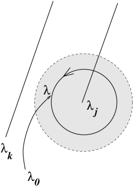
Figure 7: The paths of analytic continuation.

$$\Phi_{k}^{[-q]}(\lambda)\longmapsto\Phi_{k}^{[-q]}(\lambda)+\oint_{\gamma_{j}}d\xi_{q}\int_{\lambda_{0}}^{\xi_{q}}d\xi_{q-1}\cdots\int_{\lambda_{0}}^{\xi_{2}}d\xi_{1}~{}\phi_{k}(\xi_{1}).$$

By formula (52) it follows that the analytic continuation of $(\phi_{k})^{[-q]}(\lambda)$ along the loop $\gamma_{j}$ is

$$(\phi_{k})^{[-q]}(\lambda)\longmapsto(\phi_{k})^{[-q]}(\lambda)+\oint_{\gamma_{j}}d\xi_{q}\int_{\lambda_{0}}^{\xi_{q}}d\xi_{q-1}\cdots\int_{\lambda_{0}}^{\xi_{2}}d\xi_{1}~{}\phi_{k}(\xi_{1}),~{}~{}~{}~{}~{}~{}\forall q\geq 0.$$

Next, we express $\phi_{k}(\xi_{1})$ in terms of the solutions $\phi_{j}$ at $\lambda_{j}$. We distinguish the two cases in the lemma.

Case a): $\lambda^{\prime}_{k}\not\in\mathbb{Z}$ or $\lambda^{\prime}_{k}\in\mathbb{Z}_{-}$. We have $\phi_{k}(\xi_{1})=\vec{\Psi}_{k}(\xi_{1})$, therefore we use (4), namely

$$\phi_{k}(\xi_{1})=\left\{\matrix{\vec{\Psi}_{j}(\xi_{1})c_{jk}+\hbox{reg}(\xi_{1}-\lambda_{j}),&~{}~{}~{}~{}~{}\lambda^{\prime}_{j}\not\in\mathbb{Z}\cr\cr\vec{\Psi}_{j}(\xi_{1})\ln(\xi_{1}-\lambda_{j})~{}c_{jk}+\hbox{reg}(\xi_{1}-\lambda_{j}),&~{}~{}~{}~{}~{}\lambda^{\prime}_{j}\in\mathbb{Z}_{-}\cr\cr\left(\vec{\Psi}_{j}(\xi_{1})\ln(\xi_{1}-\lambda_{j})+{P^{(j)}(\xi_{1})\over(\xi_{1}-\lambda_{j})^{N_{j}+1}}\right)c_{jk}+\hbox{reg}(\xi_{1}-\lambda_{j}),&~{}~{}~{}~{}~{}\lambda^{\prime}_{j}=N_{j}\in\mathbb{N}}\right.$$

a.1) When $\lambda^{\prime}_{j}\not\in\mathbb{Z}$, we have

$$\oint_{\gamma_{j}}d\xi_{q}\int_{\lambda_{0}}^{\xi_{q}}d\xi_{q-1}\cdots\int_{\lambda_{0}}^{\xi_{2}}d\xi_{1}~{}\left(\vec{\Psi}_{j}(\xi_{1})c_{jk}+\hbox{reg}(\xi_{1}-\lambda_{j})\right)=$$

$$=\oint_{\gamma_{j}}d\xi_{q}~{}\Phi_{j}^{[-(q-1)]}(\xi_{q})~{}c_{jk}+\oint_{\gamma_{j}}d\xi_{q}~{}\hbox{reg}(\xi_{q}-\lambda_{j})\equiv\oint_{\gamma_{j}}d\xi_{q}~{}\Phi_{j}^{[-(q-1)]}(\xi_{q})~{}c_{jk}~{}+0,$$

because the loop integral of regular terms at $\lambda_{j}$ vanishes. Now, by (53) and (52), we have

$$\oint_{\gamma_{j}}d\xi_{q}~{}\Phi_{j}^{[-(q-1)]}(\xi_{q})~{}c_{jk}=c_{jk}~{}\Phi_{j}^{[-q]}(\xi_{q})\Big{|}_{\lambda-\lambda_{j}}^{(\lambda-\lambda_{j})e^{2\pi i}}$$

$$\equiv c_{jk}~{}\vec{\Psi}_{j}^{[-q]}(\xi_{q})\Big{|}_{\lambda-\lambda_{j}}^{(\lambda-\lambda_{j})e^{2\pi i}}~{}=\vec{\Psi}_{j}^{[-q]}(\lambda)(e^{-2\pi i\lambda^{\prime}_{j}}-1)c_{jk},~{}~{}~{}~{}~{}q\geq 0$$

The last step follows from the series representation (46). This proves the Lemma in case a.1).

a.2) When $\lambda^{\prime}_{j}\in\mathbb{Z}_{-}$, we use (54) and compute

$$\oint_{\gamma_{j}}d\xi_{q}\int_{\lambda_{0}}^{\xi_{q}}d\xi_{q-1}\cdots\int_{\lambda_{0}}^{\xi_{2}}d\xi_{1}\Bigl{(}\vec{\Psi}_{j}(\xi_{1})\ln(\xi_{1}-\lambda_{j})~{}c_{jk}+\hbox{reg}(\xi_{1}-\lambda_{j})\Bigr{)}=$$

$$=c_{jk}~{}(\vec{\Psi})_{j}^{[-q]}(\xi_{q})\ln(\xi_{q}-\lambda_{j})\Big{|}_{\lambda-\lambda_{j}}^{(\lambda-\lambda_{j})e^{2\pi i}}=2\pi ic_{jk}~{}(\vec{\Psi})_{j}^{[-q]}(\lambda),~{}~{}~{}~{}~{}~{}q\geq 0$$

This implies the Lemma in case a.2).

a.3) When $\lambda^{\prime}_{j}=N_{j}\in\mathbb{N}$, we use (55) and compute

$$\oint_{\gamma_{j}}d\xi_{q}\int_{\lambda_{0}}^{\xi_{q}}d\xi_{q-1}\cdots\int_{\lambda_{0}}^{\xi_{2}}d\xi_{1}\left[\left(\vec{\Psi}_{j}(\xi_{1})\ln(\xi_{1}-\lambda_{j})+{P^{(j)}(\xi_{1})\over(\xi_{1}-\lambda_{j})^{N_{j}+1}}\right)c_{jk}+\hbox{reg}(\xi_{1}-\lambda_{j})\right]=$$

$$=c_{jk}~{}\hat{\Psi}_{j}^{[-q+N_{j}+1]}(\xi_{q})\ln(\xi_{q}-\lambda_{j})\Big{|}_{\lambda-\lambda_{j}}^{(\lambda-\lambda_{j})e^{2\pi i}}=2\pi ic_{jk}\hat{\Psi}_{j}^{[-q+N_{j}+1]}(\lambda),~{}~{}~{}~{}~{}q\geq N_{j}+1$$

This proves the Lemma in case a.3).

Case b): when $\lambda^{\prime}_{k}=N_{k}\in\mathbb{N}$, we need to compute

$$\oint_{\gamma_{j}}d\xi_{q}\int_{\lambda_{0}}^{\xi_{q}}d\xi_{q-1}\cdots\int_{\lambda_{0}}^{\xi_{2}}d\xi_{1}\hat{\Psi}_{k}(\xi_{1}).$$ (60)

b.1) In the case of $\lambda^{\prime}_{j}\not\in\mathbb{Z}$, we use (56), and find

$$(\ref{acid})=\oint_{\gamma_{j}}d\xi_{q}\int_{\lambda_{0}}^{\xi_{q}}d\xi_{q-1}\cdots\int_{\lambda_{0}}^{\xi_{2}}d\xi_{1}\Bigl{(}\vec{\Psi}_{j}^{[-N_{k}-1]}(\xi_{1})c_{jk}+\hbox{reg}(\xi_{1}-\lambda_{j})\Bigr{)}$$

$$=\Bigl{(}c_{jk}\vec{\Psi}_{j}^{[-N_{k}-1-q]}(\xi_{q})+\hbox{reg}(\xi_{q}-\lambda_{j})\Bigr{)}\Big{|}_{(\lambda-\lambda_{j})}^{e^{2\pi i}(\lambda-\lambda_{j})}=c_{jk}(e^{-2\pi i\lambda^{\prime}_{j}}-1)\vec{\Psi}_{j}^{[-N_{k}-1-q]}(\lambda).$$

b.2) In the case of $\lambda^{\prime}_{j}\in\mathbb{N}$, we use (57) and Proposition 11, and find

$$(\ref{acid})=$$

$$\oint_{\gamma_{j}}d\xi_{q}\int_{\lambda_{0}}^{\xi_{q}}d\xi_{q-1}\cdots\int_{\lambda_{0}}^{\xi_{2}}d\xi_{1}\left[\left(\hat{\Psi}_{j}^{[N_{j}-N_{k}]}(\xi_{1})\log(\xi_{1}-\lambda_{j})+{P_{N_{j}-N_{k}-1}(\xi_{1})\over(\xi_{1}-\lambda_{j})^{N_{j}-N_{k}}}\right)c_{jk}+\hbox{reg}(\xi_{1}-\lambda_{j})\right]$$

where ${P}_{N_{j}-N_{k}-1}=0$ for $N_{k}\geq N_{j}$.

For $0\leq q\leq N_{j}-N_{k}-1$, the integral is

$$=\left[c_{jk}\left(\vec{\Psi}_{j}^{[N_{j}-N_{k}-q]}(\xi_{q})\ln(\lambda-\lambda_{j})+{P_{N_{j}-N_{k}-1-q}^{(j)}(\xi_{q})\over(\xi_{q}-\lambda_{j})^{N_{j}-N_{k}-q}}\right)+\hbox{reg}(\xi_{q}-\lambda_{j})\right]\Big{|}_{(\lambda-\lambda_{j})}^{e^{2\pi i}(\lambda-\lambda_{j})}.$$

For $q\geq N_{j}-N_{k}\geq 0$, the integral is

$$=\left[c_{jk}\vec{\Psi}_{j}^{[N_{j}-N_{k}-q]}(\xi_{q})\ln(\xi_{q}-\lambda_{j})+\hbox{reg}(\xi_{q}-\lambda_{j})\right]\Big{|}_{(\lambda-\lambda_{j})}^{e^{2\pi i}(\lambda-\lambda_{j})}.$$

In both cases, the above expressions yield

$$(\ref{acid})=2\pi ic_{jk}\vec{\Psi}_{j}^{[N_{j}-N_{k}-q]}(\lambda)$$

b.3) In case $\lambda^{\prime}_{j}\in\mathbb{Z}_{-}$, we use (58) and Proposition 11, and find

$$(\ref{acid})=\oint_{\gamma_{j}}d\xi_{q}\int_{\lambda_{0}}^{\xi_{q}}d\xi_{q-1}\cdots\int_{\lambda_{0}}^{\xi_{2}}d\xi_{1}\Bigl{(}\vec{\Psi}_{j}^{[-N_{k}-1]}(\xi_{1})\ln(\xi_{1}-\lambda_{j})c_{jk}+\hbox{reg}(\xi_{1}-\lambda_{j})\Bigr{)}$$

$$=\left[\vec{\Psi}_{j}^{[-N_{k}-1-q]}(\xi_{q})\ln(\xi_{q}-\lambda_{j})~{}c_{jk}~{}+\hbox{reg}(\xi_{q}-\lambda_{j})\right]\Big{|}_{(\lambda-\lambda_{j})}^{e^{2\pi i}(\lambda-\lambda_{j})}=2\pi ic_{jk}~{}\vec{\Psi}_{j}^{[-N_{k}-1-q]}(\lambda).$$

The above computations imply the Lemma in case b). $\Box$

Proof of Proposition 10: Given a function $f(\lambda)$, $\lambda\in{\cal P}_{\eta}$, we denote with $f_{+}(\lambda)$ the value on the left side of $L_{j}$, where $\arg(\lambda-\lambda_{j})=\eta-2\pi$. We denote with $f_{-}(\lambda)$ the value on the right side, where $\arg(\lambda-\lambda_{j})=\eta$. By Lemmas 11 and 12 we have:

$$\left({}_{\gamma}\vec{\Psi}_{k}\right)^{[-q(\lambda^{\prime}_{k})]}_{\pm}(\lambda)=F(\lambda^{\prime}_{k})\left\{\int_{\lambda_{k}}^{\lambda_{j}}(\lambda-s)^{\gamma-1}\phi_{k}^{[-q]}(s)ds~{}+\int_{\lambda_{j}}^{\lambda}(\lambda-s)^{\gamma-1}\left(\phi_{k}^{[-q]}\right)_{\pm}(s)ds\right\}$$

where

$$q(\lambda^{\prime}_{k})=\left\{\matrix{q&\hbox{ if }\lambda^{\prime}_{k}\not\in\mathbb{Z}\hbox{ or }\lambda^{\prime}_{k}\in\mathbb{Z}_{-},\cr\cr q+N_{k}+1&\hbox{ if }\lambda^{\prime}_{k}\in\mathbb{N},}\right.$$

$$\phi_{k}=\left\{\matrix{\vec{\Psi}_{k}&\hbox{ if }\lambda^{\prime}_{k}\not\in\mathbb{Z}\hbox{ or }\lambda^{\prime}_{k}\in\mathbb{Z}_{-},\cr\cr\hat{\Psi}_{k}&\hbox{ if }\lambda^{\prime}_{k}\in\mathbb{N},}\right.$$

$$F(\lambda^{\prime}_{k})=\left\{\matrix{{\sin\pi\lambda^{\prime}_{k}\over\Gamma(\gamma)\sin\pi(\lambda^{\prime}_{k}-\gamma)}&\hbox{ if }\lambda^{\prime}_{k}\not\in\mathbb{Z},\cr\cr{\pi\over\Gamma(\gamma)\sin\pi\gamma}&\hbox{ if }\lambda^{\prime}_{k}\in\mathbb{Z}.}\right.$$

In the integral, $\arg(\lambda-s)$, $s\in{\cal P}_{\eta}$, has the value obtained by the continuous change along the path of integration from $\lambda_{k}$ up to $s$ belonging to $L_{j}$. Change from $f_{-}$ to $f_{+}$ is obtained along a small loop encircling only $\lambda_{j}$. Therefore, Lemma 12 yields

$$\left({}_{\gamma}\vec{\Psi}_{k}\right)^{[-q(\lambda^{\prime}_{k})]}_{-}(\lambda)-\left({}_{\gamma}\vec{\Psi}_{k}\right)^{[-q(\lambda^{\prime}_{k})]}_{+}(\lambda)=\alpha_{j}[\gamma]c_{jk}[\gamma]\left({}_{\gamma}\vec{\Psi}_{j}\right)^{[-q(\lambda^{\prime}_{k})]}_{+}(\lambda).$$ (61)

By Lemmas 11 and 12 we write

$$\left({}_{\gamma}\vec{\Psi}_{k}\right)^{[-q(\lambda^{\prime}_{k})]}_{-}(\lambda)-\left({}_{\gamma}\vec{\Psi}_{k}\right)^{[-q(\lambda^{\prime}_{k})]}_{+}(\lambda)=F(\lambda^{\prime}_{k})\int_{\lambda_{j}}^{\lambda}(\lambda-s)^{\gamma-1}\left[\left(\phi_{k}^{[-q]}\right)_{-}(s)-\left(\phi_{k}^{[-q]}\right)_{+}(s)\right]$$ (62)

We need to distinguish two cases.

1) $\lambda^{\prime}_{k}\not\in\mathbb{Z}$, or $\lambda^{\prime}_{k}\in\mathbb{Z}_{-}$. In this case (61), (62) and Lemma 12 applied to the integrand yield the following equalities.

1.a) for $\lambda^{\prime}_{j}\not\in\mathbb{Z}$ or $\lambda^{\prime}_{j}\in\mathbb{Z}_{-}$:

$$\alpha_{j}[\gamma]c_{jk}[\gamma]\left({}_{\gamma}\vec{\Psi}_{j}\right)^{[-q]}_{+}(\lambda)=F(\lambda^{\prime}_{k})\int_{\lambda_{j}}^{\lambda}ds~{}(\lambda-s)^{\gamma-1}\alpha_{j}c_{jk}\left(\vec{\Psi}_{j}\right)^{[-q]}_{+}(s),$$ (63)

1.b) for $\lambda^{\prime}_{j}\in\mathbb{N}$:

$$\alpha_{j}[\gamma]c_{jk}[\gamma]\left({}_{\gamma}\vec{\Psi}_{j}\right)^{[-q]}_{+}(\lambda)=F(\lambda^{\prime}_{k})\int_{\lambda_{j}}^{\lambda}ds~{}(\lambda-s)^{\gamma-1}\alpha_{j}c_{jk}\left(\hat{\Psi}_{j}\right)^{[-q+N_{j}+1]}_{+}(s),$$ (64)

We apply again Lemmas (11) and (12) to express the r.h.s. of the above equalities. To this end, we need $(\lambda-s)_{+}$ in the integrand. Observe that

$$(\lambda-s)^{\gamma-1}\hbox{ in the integrand }=\left\{\matrix{~{}~{}(\lambda-s)_{-}^{\gamma-1}=\left[e^{2\pi i}(\lambda-s)_{+}\right]^{\gamma-1}&\hbox{ when }k\succ j\cr\cr(\lambda-s)_{+}^{\gamma-1}&\hbox{ when }k\prec j.}\right.$$

Indeed, when $\lambda$ belongs to the left side of $L_{j}$ and $s\in{\cal P}_{\eta}$, then $\eta-2\pi<\arg(\lambda-s)<\eta$. When $s$ reaches $L_{j}$ from the left, then $\arg(\lambda-s)\to\eta$ if $L_{k}$ is to the left of $L_{j}$, namely $k\succ j$: in this case we obtain $(\lambda-s)_{-}$. On the other hand, $\arg(\lambda-s)\to\eta-2\pi$ if $L_{k}$ is to the right of $L_{j}$, namely $k\prec j$: in this case we obtain $(\lambda-s)_{+}$. See figure 8.

Figure 8: The figure shows $\arg(\lambda-s)$ as $s\to\lambda_{j}$.

Applying Lemmas (11) and (12) we find

$$\hbox{r.h.s. of (\ref{tm3}) and (\ref{tm4}) }=\left\{\matrix{{F(\lambda^{\prime}_{k})\over F(\lambda^{\prime}_{j})}e^{2\pi i\gamma}\alpha_{j}c_{jk}\left({}_{\gamma}\vec{\Psi}_{j}\right)_{+}^{[-q]}(\lambda)&k\succ j,\cr\cr{F(\lambda^{\prime}_{k})\over F(\lambda^{\prime}_{j})}\alpha_{j}c_{jk}\left({}_{\gamma}\vec{\Psi}_{j}\right)_{+}^{[-q]}(\lambda)&k\prec j.}\right.$$

Namely:

$$\alpha_{j}[\gamma]c_{jk}[\gamma]=\left\{\matrix{{F(\lambda^{\prime}_{k})\over F(\lambda^{\prime}_{j})}e^{2\pi i\gamma}\alpha_{j}c_{jk}&k\succ j,\cr\cr{F(\lambda^{\prime}_{k})\over F(\lambda^{\prime}_{j})}\alpha_{j}c_{jk}&k\prec j.}\right.$$ (65)

Finally, we compute the ratio $F(\lambda^{\prime}_{k})/F(\lambda^{\prime}_{j})$. For $\lambda^{\prime}_{j}\not\in\mathbb{Z}$:

$${F(\lambda^{\prime}_{k})\over F(\lambda^{\prime}_{j})}={\sin\pi\lambda^{\prime}_{k}~{}\sin\pi(\lambda^{\prime}_{j}-\gamma)\over\sin\pi\lambda^{\prime}_{j}~{}\sin\pi(\lambda^{\prime}_{k}-\gamma)}={(1-e^{-2\pi i\lambda^{\prime}_{k}})(1-e^{-2\pi i(\lambda^{\prime}_{j}-\gamma)})\over(1-e^{-2\pi i\lambda^{\prime}_{j}})(1-e^{-2\pi i(\lambda^{\prime}_{k}-\gamma)})}={\alpha_{k}\alpha_{j}[\gamma]\over\alpha_{j}\alpha_{k}[\gamma]}.$$

For $\lambda^{\prime}_{j}\in\mathbb{Z}$:

$${F(\lambda^{\prime}_{k})\over F(\lambda^{\prime}_{j})}={\sin\pi\gamma~{}\sin\pi\lambda^{\prime}_{k}\over\pi~{}\sin\pi(\lambda^{\prime}_{k}-\gamma)}={e^{2\pi i\gamma}-1\over 2\pi i}{e^{-2\pi i\lambda^{\prime}_{k}}-1\over e^{-2\pi i(\lambda^{\prime}_{k}-\gamma)}-1}={\alpha_{j}[\gamma]\over\alpha_{j}}{\alpha_{k}\over\alpha_{k}[\gamma]}$$

where we have used the fact that $\alpha_{j}=2\pi i$ and $\alpha_{j}[\gamma]=e^{2\pi i\gamma}-1$.

The above computations imply the statement of Proposition 10 when $\lambda^{\prime}_{k}\not\in\mathbb{Z}$ and $\lambda^{\prime}_{k}\in\mathbb{Z}_{-}$.

2) $\lambda^{\prime}_{k}\in\mathbb{N}$. In this case (61), (62) and Lemma 12 applied to the integrand yield the following equalities.

2.a) for $\lambda^{\prime}_{j}\not\in\mathbb{Z}$ or $\lambda^{\prime}_{j}\in\mathbb{Z}_{-}$:

$$\alpha_{j}[\gamma]c_{jk}[\gamma]\left({}_{\gamma}\vec{\Psi}_{j}\right)^{[-q-N_{k}-1]}_{+}(\lambda)=F(\lambda^{\prime}_{k})\int_{\lambda_{j}}^{\lambda}ds~{}(\lambda-s)^{\gamma-1}\alpha_{j}c_{jk}\left(\vec{\Psi}_{j}\right)^{[-q-N_{k}-1]}_{+}(s)$$ (66)

2.b) for $\lambda^{\prime}_{j}\in\mathbb{N}$:

$$\alpha_{j}[\gamma]c_{jk}[\gamma]\left({}_{\gamma}\vec{\Psi}_{j}\right)^{[-q-N_{k}-1]}_{+}(\lambda)=F(\lambda^{\prime}_{k})\int_{\lambda_{j}}^{\lambda}ds~{}(\lambda-s)^{\gamma-1}\alpha_{j}c_{jk}\left(\hat{\Psi}_{j}\right)^{[-q-N_{k}-1+N_{j}+1]}_{+}(s).$$ (67)

We apply again Lemmas (11) and (12) to express the r.h.s. of the above equalities, keeping into account the branch of $(\lambda-s)^{\gamma-1}$ as before. We find

$$\hbox{r.h.s. of (\ref{tm5}) and (\ref{tm6}) }=\left\{\matrix{{F(\lambda^{\prime}_{k})\over F(\lambda^{\prime}_{j})}e^{2\pi i\gamma}\alpha_{j}c_{jk}\left({}_{\gamma}\vec{\Psi}_{j}\right)_{+}^{[-q-N_{k}-1]}(\lambda)&k\succ j,\cr\cr{F(\lambda^{\prime}_{k})\over F(\lambda^{\prime}_{j})}\alpha_{j}c_{jk}\left({}_{\gamma}\vec{\Psi}_{j}\right)_{+}^{[-q-N_{k}-1]}(\lambda)&k\prec j.}\right.$$

Namely, we obtain again

$$\alpha_{j}[\gamma]c_{jk}[\gamma]=\left\{\matrix{{F(\lambda^{\prime}_{k})\over F(\lambda^{\prime}_{j})}e^{2\pi i\gamma}\alpha_{j}c_{jk}&k\succ j,\cr\cr{F(\lambda^{\prime}_{k})\over F(\lambda^{\prime}_{j})}\alpha_{j}c_{jk}&k\prec j.}\right.$$ (68)

Finally, we compute the ratio $F(\lambda^{\prime}_{k})/F(\lambda^{\prime}_{j})$. For $\lambda^{\prime}_{j}\not\in\mathbb{Z}$:

$${F(\lambda^{\prime}_{k})\over F(\lambda^{\prime}_{j})}={\pi\over\sin\pi\gamma}{\sin\pi(\lambda^{\prime}_{j}-1)\over\sin\pi\lambda^{\prime}_{j}}={2\pi i\over e^{2\pi i\gamma}-1}{e^{-2\pi i(\lambda^{\prime}_{j}-\gamma)}-1\over e^{-2\pi i\lambda^{\prime}_{j}}-1}={\alpha_{k}\over\alpha_{k}[\gamma]}{\alpha_{j}[\gamma]\over\alpha_{j}}$$

where we have used the fact that $\alpha_{k}=2\pi i$ and $\alpha_{k}[\gamma]=e^{2\pi i\gamma}-1$.

For $\lambda^{\prime}_{j}\in\mathbb{Z}$:

$${F(\lambda^{\prime}_{k})\over F(\lambda^{\prime}_{j})}=1$$

In this last case, observe that $\alpha_{k}=\alpha_{j}=2\pi i$ and $\alpha_{k}[\gamma]=\alpha_{j}[\gamma]=e^{2\pi i\gamma}-1$.

The above computations imply the statement of Proposition 10 when $\lambda^{\prime}_{k}\in\mathbb{N}$. $\Box$

8 Appendix

Some statements of the main body of the paper are proved in [3] with the assumption (i) of [3], namely $\lambda^{\prime}_{1},...,\lambda^{\prime}_{n}$ not integers. Here we prove the statements without assumptions on $A_{1}$.

Proof of Proposition 1: It goes as the proof of Proposition 1 in [3], which was done assuming no integer $\lambda^{\prime}_{k}$’s, $k=1,...,n$. We repeat the proof with no assumptions on the $\lambda^{\prime}_{k}$’s. For the proof, recall Remark 1 and Lemma 2.

Vector solutions of the equation (2) form a $n$ dimensional linear space. In Section 2 we have proved that for any $j=1,...,n$, the vector solutions regular at one $\lambda_{j}$ form a linear space $V_{j}$ of dimension dim$V_{j}\geq n-1$. Now, choose a $\lambda_{k}$. The number of independent solutions which are regular at each of the $n-1$ poles $\lambda_{j}\neq\lambda_{k}$ is equal to dim$(\cap_{j\neq k}V_{j})\geq 1$. Therefore, there exist at least one vector solutions $\vec{\Psi}^{*}_{k}(\lambda)$, analytic at all $\lambda_{j}\neq\lambda_{k}$, $1\leq j\leq n$, $j\neq k$.

If dim$(\cap_{j\neq k}V_{j})>1$, then there must exist a polynomial solution of (2). Indeed, suppose that dim$(\cap_{j\neq k}V_{j})>1$. So there are at least two independent solutions, regular at each $\lambda_{j}\neq\lambda_{k}$. Let them be $\vec{\psi}_{1}(\lambda)$ and $\vec{\psi}_{2}(\lambda)$. At $\lambda_{k}$ they must have representation $\vec{\psi}_{q}=c_{q}~{}\vec{\Psi}_{k}^{(sing)}+\hbox{reg}_{q}(\lambda-\lambda_{k})$, $q=1,2$, $c_{q}\in\mathbb{C}\backslash\{0\}$. But now, $c_{1}^{-1}\vec{\psi}_{1}-c_{2}^{-1}\vec{\psi}_{2}$ is not vanishing (by independence of the two solutions) and is analytic also at $\lambda=\lambda_{k}$. It follows that there is an analytic solution at each $\lambda_{i}$, $1\leq i\leq n$, which therefore must be polynomial (Remark 1). This can occur if and only if $A_{1}$ has at least one negative integer eigenvalue (Lemma 2). Thus, if we assume that $A_{1}$ has no negative integer eigenvalues, so that there are no polynomial solutions, then dim$(\cap_{j\neq k}V_{j})=1$. Therefore, for any $k$ there exists a unique (up to normalization) solution which is regular at all $\lambda_{j}\neq\lambda_{k}$ and must be singular at $\lambda_{k}$. It is the unique $\vec{\Psi}_{k}^{*}$ with normalization (16). Obviously, $\vec{\Psi}_{1}^{*},...,\vec{\Psi}_{n}^{*}$ are independent. In particular, observe that if $\lambda^{\prime}_{k}\in-\mathbb{N}-2$, necessarily the log-singular solution must exist (i.e. $\vec{\Psi}_{k}^{(sing)}\neq 0$).

Conversely, if $\vec{\Psi}_{1}^{*}(\lambda),...,\vec{\Psi}_{n}^{*}(\lambda)$ exist satisfying (15) and (16), then they are independent, because $\sum_{l=1}^{n}c_{l}\vec{\Psi}_{l}^{*}(\lambda)=0$ holds when $\lambda\to\lambda_{i}$, $\forall i=1,...,n$, only if $c_{i}=0$. Moreover, $\sum_{l=1}^{n}c_{l}\vec{\Psi}_{l}^{*}(\lambda)$ is analytic at all $\lambda_{j}\neq\lambda_{k}$ for a chosen $k$, only if $c_{j}=0$ for all $j\neq k$. Therefore, there is only one solution analytic at all $\lambda_{j}\neq\lambda_{k}$, which is a multiple of $\vec{\Psi}_{k}^{*}(\lambda)$. In other words, the space $\cap_{j\neq k}V_{j}$ of solutions regular at all $\lambda_{j}\neq\lambda_{k}$ is one dimensional, thus there are no polynomial solutions and $A_{1}$ cannot have a negative integer eigenvalue.

To prove the last assertion, write $\Psi(\lambda)=\Psi^{*}(\lambda)\tilde{C}$. Thus $\vec{\Psi}_{k}(\lambda)=\vec{\Psi}_{k}^{*}(\lambda)\tilde{C}_{kk}+\sum_{j\neq k}\vec{\Psi}_{j}^{*}(\lambda)\tilde{C}_{jk}$. Now, consider the behaviours at $\lambda=\lambda_{k}$ of l.h.s. and r.h.s. By (12), (15) and (16) we conclude that $\tilde{C}_{kk}=1$ in case $\lambda^{\prime}_{k}\not\in\mathbb{Z}$, and $\tilde{C}_{kk}=0$ in cases $\lambda^{\prime}_{k}\in\mathbb{Z}$. Thus $\tilde{C}_{kk}=c_{kk}$. Now consider the behaviours at $\lambda=\lambda_{j}$, $j\neq k$, of l.h.s. and r.h.s. By (4), (15) and (16) we obtain $\tilde{C}_{jk}=c_{jk}$. $\Box$

Proof of Proposition 5: i) is immediate, because if $\lambda_{k}$ is accessible and $\lambda\in{\cal P}_{\eta}\cap{\cal P}_{\tilde{\eta}}$, then $\vec{\Psi}_{k}^{(k)}(\lambda,\eta)$ and $\vec{\Psi}_{k}^{(k)}(\lambda,\tilde{\eta})$ are the same branch. The same holds for the solutions $\vec{\Psi}_{k}$.

ii) and iii) are proved noticing that $\lambda_{1},...,\lambda_{n}$ are all accessible from ${\cal P}_{\eta}\cap{\cal P}_{\tilde{\eta}}$, therefore i) holds for any $k$. Thus $C(\eta)=C(\tilde{\eta})$. From Proposition 1 we see that $\Psi^{*}$ is uniquely defined starting from the $\vec{\Psi}_{k}$’s and $C$. $\Box$

Proof of Proposition 6: The proof follows that of Proposition 4 of [3], here generalized to the general case when $\lambda^{\prime}_{1},...,\lambda^{\prime}_{k}$ are any complex numbers.

Choose a $\lambda_{k}$. In the plane ${\cal P}_{\eta}$ add the cut $\arg(\lambda-\lambda_{k})=\tilde{\eta}$. Pet $\Pi_{\eta,\tilde{\eta}}^{k}$ be the connected region given by the reference points relative to these cuts, namely all points satisfying both conditions $\eta-2\pi<\arg(\lambda-\lambda_{j})<\eta$, $\forall j=1,..,n$, and $\tilde{\eta}-2\pi<\arg(\lambda-\lambda_{k})<\tilde{\eta}$. See figure 9. We have then a relation between fundamental matrices

$$\vec{\Psi}_{k}^{*}(\lambda,\tilde{\eta})=\sum_{j=1}^{n}\vec{\Psi}_{j}^{*}(\lambda,{\eta})~{}W_{jk},~{}~{}~{}~{}~{}\lambda\in\Pi_{\eta,\tilde{\eta}}^{k}.$$

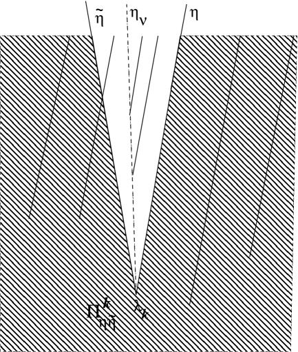
Figure 9: The connected region $\Pi_{\eta,\tilde{\eta}}^{k}$

– If $\lambda_{j}$ is accessible and $j\neq k$, then $W_{jk}=0$, because $\vec{\Psi}_{j}^{*}(\lambda,{\eta})$ is singular at $\lambda_{j}$ and $\vec{\Psi}_{k}^{*}(\lambda,\tilde{\eta})$ is not. Both are the same branch.

– At $\lambda_{k}$, both $\vec{\Psi}_{k}^{*}(\lambda,\tilde{\eta})$ and $\vec{\Psi}_{k}^{*}(\lambda,\tilde{\eta})$ have the same singular behavior with the same branch of logarithm (Proposition 1), therefore $\vec{\Psi}_{k}^{*}(\lambda,\tilde{\eta})=\vec{\Psi}_{k}^{*}(\lambda,\tilde{\eta})+$reg$(\lambda-\lambda_{k})$. This implies $W_{kk}=1$. Thus

$$\vec{\Psi}_{k}^{*}(\lambda,\tilde{\eta})=\vec{\Psi}_{k}^{*}(\lambda,{\eta})+\sum_{j~{}not~{}acc.}\vec{\Psi}_{j}^{*}(\lambda,{\eta})~{}W_{jk},~{}~{}~{}~{}~{}\lambda\in\Pi_{\eta,\tilde{\eta}}^{k}.$$ (69)

where the sum is on indexes of non accessible points.

– If $\lambda_{j}$ is not accessible, in order to access it and evaluate the behaviour of l.h.s. and r.h.s. of (69), we need to analytically continue the r.h.s beyond the cut $\arg(\lambda-\lambda_{k})=\eta$, crossing it in anticlockwise direction. The l.h.s is already defined beyond this cut. Also, all $\vec{\Psi}_{j}^{*}(\lambda,{\eta})$ for $\lambda_{j}$ not accessible are already defined beyond this cut. Therefore, after crossing the cut, only $\vec{\Psi}_{k}^{*}(\lambda,{\eta})$ is analytically continued by $M_{k}^{*}$, according to Proposition 2, and (69) becomes

$$\vec{\Psi}_{k}^{*}(\lambda,\tilde{\eta})=m_{kk}\vec{\Psi}_{k}^{*}(\lambda,{\eta})+\alpha_{k}\sum_{j\neq k}c_{jk}\vec{\Psi}_{j}^{*}(\lambda,{\eta})+\sum_{j~{}not~{}acc.}\vec{\Psi}_{j}^{*}(\lambda,{\eta})~{}W_{jk}$$

Since the l.h.s is not singular at inaccessible points, we conclude that $W_{jk}=-\alpha_{k}c_{jk}$, for any inaccessible $\lambda_{j}$. Finally, we note that the inaccessible points are those such that $\arg(\lambda_{j}-\lambda_{k})=\eta_{\nu}$. We also see that $j\succ k$ w.r.t $\eta$.

The same argument is repeated for any $k$.

As for $W_{\nu}^{-1}$, the argument does not change, but this time $C$ and $M_{k}^{*}$ are referred to $\tilde{\eta}$. $\Box$

Proof of Lemma 4: If we write $\lambda_{\eta}$ if $\lambda\in{\cal P}_{\eta}$. Then

$$\lambda_{\eta}-\lambda_{k}=(\lambda_{\eta-2\pi}-\lambda_{k})e^{2\pi i}$$

It follows from the definition of $\Psi$ that, whatever the values $\lambda^{\prime}_{1},...,\lambda^{\prime}_{n}$ are, we have

$$\Psi(\lambda,\eta-2\pi)=\Psi(\lambda,\eta)e^{2\pi i\Lambda^{\prime}}.$$

on the universal covering of $\mathbb{C}\backslash\{\lambda_{1},...,\lambda_{n}\}$. From the above and the connection relations we have

$$\vec{\Psi}_{k}(\lambda,\eta)=\vec{\Psi}_{j}^{(sing)}(\lambda,\eta)~{}c_{jk}(\eta)+\hbox{reg}(\lambda-\lambda_{j}),$$

and

$$\vec{\Psi}_{k}(\lambda,\eta)=e^{-2\pi i\lambda^{\prime}_{k}}\vec{\Psi}_{k}(\lambda,\eta-2\pi)=$$

$$=e^{-2\pi i\lambda^{\prime}_{k}}~{}\vec{\Psi}_{j}^{(sing)}(\lambda,\eta-2\pi)~{}c_{jk}(\eta-2\pi)+\hbox{reg}(\lambda-\lambda_{j}),$$

Now we use the fact that $\vec{\Psi}_{j}^{(sing)}(\lambda,\eta-2\pi)=\vec{\Psi}_{j}(\lambda,\eta-2\pi)$ when $\lambda^{\prime}_{j}\not\in\mathbb{Z}$, and when $\lambda^{\prime}_{j}\in\{-1\}\cup\mathbb{N}$ we have

$$\vec{\Psi}_{j}^{(j)}(\lambda,\eta-2\pi)=\vec{\Psi}_{j}(\lambda,\eta-2\pi)\left[\ln(\lambda_{\eta-2\pi}-\lambda_{j})+{P^{(j)}_{N_{j}}(\lambda_{\eta-2\pi})\over(\lambda-\lambda_{j})^{N_{j}+1}}\right]+\hbox{reg}(\lambda_{\eta-2\pi}-\lambda_{j})$$

$$=e^{2\pi i\lambda^{\prime}_{j}}\vec{\Psi}_{j}(\lambda,\eta)\left\{\left[\ln(\lambda_{\eta}-\lambda_{j})-2\pi i\right]+{P^{(j)}_{N_{j}}(\lambda_{\eta})\over(\lambda-\lambda_{j})^{N_{j}+1}}\right\}+\hbox{reg}(\lambda_{\eta}-\lambda_{j})$$

$$=e^{2\pi i\lambda^{\prime}_{j}}\vec{\Psi}_{j}^{(sing)}(\lambda,\eta)+\hbox{reg}(\lambda-\lambda_{j}).$$

The last step is due to the fact that $\vec{\Psi}_{j}(\lambda,\eta)$ is analytic at $\lambda_{j}$ (note that $e^{2\pi i\lambda^{\prime}_{j}}=1$) and is absorbed into $\hbox{reg}(\lambda-\lambda_{j})$. Therefore, in all cases we have (in full generality, taking $P^{(j)}_{N_{j}}\equiv 0$ when $\lambda^{\prime}_{j}\in\mathbb{Z}_{-}$):

$$\vec{\Psi}_{j}^{(sing)}(\lambda,\eta)~{}c_{jk}(\eta)+\hbox{reg}(\lambda-\lambda_{j})=e^{2\pi i(\lambda^{\prime}_{j}-\lambda^{\prime}_{k})}~{}\vec{\Psi}_{j}^{(sing)}(\lambda,\eta)~{}c_{jk}(\eta-2\pi)+\hbox{reg}(\lambda-\lambda_{j}).$$

Finally, since $\vec{\Psi}_{j}^{(sing)}(\lambda,\eta)$ is singular at $\lambda_{j}$, the statement of the lemma follows. $\Box$

Proof of Proposition 7: Compared to [3], we only need to consider more general monodromy matrices. Relation (22) is

$$\vec{\Psi}_{k}^{*}(\lambda,\eta-\pi)=\sum_{j=1}^{n}\vec{\Psi}_{j}^{*}(\lambda,\eta)C_{jk}^{+},~{}~{}~{}\lambda\in{\Pi}_{\eta,\eta-\pi}^{k}$$

See proof of Proposition 6 for the definition of ${\Pi}_{\eta,\eta-\pi}^{k}$. See also figure 10.

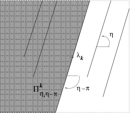
Figure 10: The connected region $\Pi_{\eta,\eta-\pi}^{k}$, branch cuts at angle $\eta$ and one branch cut at angle $\eta-\pi$ at $\lambda_{k}$

- If $\lambda_{j}\neq\lambda_{k}$ is accessible, it means that $j\succ k$. At $\lambda_{j}$, $\vec{\Psi}_{j}^{*}(\lambda,\eta)$ is singular, while $\vec{\Psi}_{k}^{*}(\lambda,\eta-\pi)$ is not. Both have the same branch of $\ln(\lambda-\lambda_{j})$, so we must conclude that $C_{jk}^{+}=0$.

- At $\lambda_{k}$, $\vec{\Psi}_{k}^{*}(\lambda,\eta)$ and $\vec{\Psi}_{k}^{*}(\lambda,\eta-\pi)$ are both singular with the same branch of $\ln(\lambda-\lambda_{k})$, so we must conclude that $C_{kk}^{+}=1$.

- If $\lambda_{j}\neq\lambda_{k}$ is not accessible, it means that $j\prec k$. The l.h.s. is define also at $\lambda_{j}$, while the r.h.s. needs analytic continuation in order to reach $\lambda_{j}$. The continuation is given by $\Psi^{*}(\lambda,\eta)\mapsto\Psi^{*}(\lambda,\eta)(M_{k}^{*}(\eta))^{-1}$. therefore

$$\vec{\Psi}_{k}^{*}(\lambda,\eta-\pi)=\vec{\Psi}_{k}^{*}(\lambda,\eta)e^{2\pi i\lambda^{\prime}_{k}}+\sum_{l\neq k}\beta_{k}c_{lk}(\eta)~{}\vec{\Psi}_{l}^{*}(\lambda,\eta)+\sum_{j~{}not~{}access.}\vec{\Psi}_{j}^{*}(\lambda,\eta)C_{jk}^{+}.$$

Since $\vec{\Psi}_{k}^{*}(\lambda,\eta-\pi)$ is not singular at a non accessible $\lambda_{j}$ , while $\vec{\Psi}_{l}^{*}(\lambda,\eta)$ is, we conclude that $C_{jk}^{+}+\beta_{k}c_{jk}(\eta)=0$.

The same reasoning is repeated for (23). This time the monodromy which gives analytic continuation is $M_{k}^{*}(\eta-2\pi)$. Thus, we obtain that $C_{jk}^{-}=-\alpha_{k}c_{jk}(\eta-2\pi)$ when $j\succ k$ (non accessible case), $C_{jk}^{-}=0$ for $j\prec k$ (accessible case) and $C_{kk}^{-}=1$ . Then, we use Lemma 4. $\Box$

References

- [1] W. Balser: Birkhoff’s reduction Problem. Russian Math. Surveys 59:6 (2004), 1047-1059.
- [2] W.Balser, W.B.Jurkat, D.A.Lutz: Birkhoff Invariants and Stokes’ Multipliers for Meromorphic Linear Differential Equations, Journal Math. Analysis and Applications, 71, (1979), 48-94.
- [3] W. Balser, W. B. Jurkat, D. A. Lutz: On the reduction of connection problems for differential equations with an irregular singular point to ones with only regular singularities, I, SIAM J. Math. Anal. Vol 12, No 5, (1981), 691-721.
- [4] G. D. Birkhoff: Singular points of ordinary linear differential equations, Trans. Amer. Math. Soc. 10 (1909), 436-470.
- [5] G. Doetsch: Introduction to the Theory and Application of the Laplace Transformation. Springer (1974)
- [6] B.Dubrovin: Geometry of 2D topological field theories, Lecture Notes in Math, 1620, (1996), 120-348.
- [7] B.Dubrovin: Painlevé trascendents in two-dimensional topological field theory, in “The Painlevé Property, One Century later” edited by R.Conte, Springer (1999).
- [8] B.Dubrovin: On almost duality for Frobenius manifolds, in Geometry, Topology, and Mathematical Physics, Amer. Math. Soc. Transl. Ser. 2, (2004), 75-132. arXiv: math/0307374v2 (2004).
- [9] S. Galkin, V. Golyshev, H. Iritani: Gamma Classes and Quantum Cohomology of Fano Manifolds: Gamma Conjectures. arXiv: 1404.6407 [math.AG] (2014)
- [10] E.L. Ince: Ordinary differential equations. Dover, (1956).
- [11] M. Loday-Richaud, P. Remy: Resurgence, Stokes phenomenon and alien derivatives for level-one linear differential systems. J. Differential Equations 250, (2011), 1591-1630.
- [12] M. Mazzocco: Painlevé sixth equation as isomonodromy deformations equations of an irregular system, in: The Kowalewski property, CRM Proceedings and Lecture Notes 32:221–240 (2002).
- [13] W. Wasow: Asymptotic Expansions for Ordinary Differential Equations, Dover