Comparison of multivariate distributions using quantile–quantile plots and related tests

Abstract

The univariate quantile–quantile (Q–Q) plot is a well-known graphical tool for examining whether two data sets are generated from the same distribution or not. It is also used to determine how well a specified probability distribution fits a given sample. In this article, we develop and study a multivariate version of the Q–Q plot based on the spatial quantile. The usefulness of the proposed graphical device is illustrated on different real and simulated data, some of which have fairly large dimensions. We also develop certain statistical tests that are related to the proposed multivariate Q–Q plot and study their asymptotic properties. The performance of those tests are compared with that of some other well-known tests for multivariate distributions available in the literature.

,
and

1 Introduction

The univariate quantile–quantile (Q–Q) plot is a diagnostic tool, which is widely used to assess the distributional similarities and differences between two independent samples (see, e.g., Gnanadesikan and Wilk [18], Gnanadesikan [17] and Chambers et al. [9]). As discussed in Doksum [12], Doksum and Sievers [13] and Koenker ([23], pages 31 and 32), there are some fundamental connections between the Q–Q plot and the two-sample problem involving a semi-parametric treatment effect model. The Q–Q plot is also a popular device for checking the appropriateness of a specified probability distribution for a given univariate data. While the univariate Q–Q plot has a long history as a graphical tool for data analysis, there are only limited attempts in the literature to generalize the Q–Q plot for multivariate samples. One can construct the Q–Q plot for multivariate data using the marginal quantiles. However, a Q–Q plot based on the marginal quantiles fails to capture the nature of dependence among the marginals of a multivariate distribution. Such a Q–Q plot can only compare the marginal distributions, but it is inadequate for a proper comparison of two multivariate distributions because the marginal quantiles do not characterize a multivariate distribution (see the supplemental article (Dhar, Chakraborty and Chaudhuri [11]) for an illustrative example).

Breckling and Chambers [7], Chaudhuri [10] and Koltchinskii [24] extensively studied a multivariate quantile, which is popularly known as the spatial quantile. Koltchinskii ([24], Corollary 2.9, page 446) established that these spatial quantiles characterize multivariate distributions. In this article, we propose an extension of the Q–Q plot using the spatial quantiles for multivariate data. As we will see in subsequent sections, these Q–Q plots are in many ways natural generalizations of the univariate Q–Q plot. In particular, for a $d$-dimensional multivariate data, there will be $d$ two-dimensional plots, where the points in each plot cluster around a straight line with slope $=1$ and intercept $=0$ if and only if the two multivariate distributions under comparison are identical.

Motivated by the one-sample Q–Q plot, Shapiro and Wilk [33] proposed a test for normality of univariate data. We also propose and study some statistical tests for multivariate distributions, which are related to our multivariate Q–Q plots. In our numerical and asymptotic studies, those tests turn out to have either comparable or superior performance when compared with the Kolmogorov–Smirnov and the Cramer–von Mises tests for multivariate distributions.

2 Multivariate Q–Q plots

Recall that a univariate Q–Q plot based on two samples with sizes $n$ and $m$ consists of $r$ ($r=n+m$ if $n\neq m$ and $r=n$ if $n=m$) points in the two-dimensional plane, where for $i=1,2,\ldots,r$, the two coordinates of the $i$th point are the $(i/r)$th quantiles of the two samples. Here, in order to compare the quantiles, one has to match the quantiles of one data set with the corresponding quantiles of another data set. Easton and McCulloch [14] made an attempt to solve a similar matching problem for multivariate data. Their procedure was based on the permutation of the data that produced the minimum sum of the Euclidean distances between the matching data points in the two given samples. Consequently, in order to assess how well a specified probability distribution fits a given multivariate sample, they used a sample simulated from the specified distribution. The Q–Q plots proposed by them can be used in two-sample problems only if the two samples have the same size. In this paper, we use a matching procedure based on the spatial rank and the spatial quantile. The procedure is computationally simple and can be used in a two-sample problem even if the two samples do not have the same size. Further, in the case of a one-sample problem, where one tries to test whether a specified distribution fits the data well or not, the construction of our Q–Q plot does not require generation of a sample from the specified distribution.

The spatial rank of ${\mathbf{z}}\in\mathbb{R}^{d}$ with respect to the data cloud formed by the observations ${\cal{X}}=\{{\mathbf{x}}_{1},\ldots,{\mathbf{x}}_{n}\}$ is defined as $n^{-1}\sum_{i:{\mathbf{x}}_{i}\neq{\mathbf{z}}}\|{\mathbf{z}}-{\mathbf{x}}_{i}\|^{-1}({\mathbf{z}}-{\mathbf{x}}_{i})$ (see, e.g., Möttönen and Oja [29], Chaudhuri [10] and Serfling [32]). For a random vector ${\mathbf{x}}$ with a probability distribution $F$ on $\mathbb{R}^{d}$, the $d$-dimensional spatial quantile $Q_{F}({\mathbf{u}})=(Q_{F,1}({\mathbf{u}}),\ldots,Q_{F,d}({\mathbf{u}}))$ is defined as $Q_{F}({\mathbf{u}})=\arg\min_{Q\in\mathbb{R}^{d}}E\{\Phi({\mathbf{u}},{\mathbf{x}}-Q)-\Phi({\mathbf{u}},{\mathbf{x}})\}$ (see Chaudhuri [10] and Koltchinskii [24]). Here $\Phi({\mathbf{u}},{\mathbf{s}})=\|{\mathbf{s}}\|+\langle{\mathbf{u}},{\mathbf{s}}\rangle$, ${\mathbf{u}}\in B^{d}=\{{\mathbf{v}}\colon\ {\mathbf{v}}\in\mathbb{R}^{d},\|{\mathbf{v}}\|<1\}$, $\langle\cdot,\cdot\rangle$ is the Euclidean inner product, and $\|\cdot\|$ is the Euclidean norm induced by the inner product. For a random sample ${\cal{X}}=\{{\mathbf{x}}_{1},\ldots,{\mathbf{x}}_{n}\}$, the empirical spatial quantile $Q_{{\cal{X}}}({\mathbf{u}})=(Q_{{\cal{X}},1}({\mathbf{u}}),\ldots,Q_{{\cal{X}},d}({\mathbf{u}}))$ is obtained by replacing $F$ with its empirical version $F_{n}$. When different coordinate variables in a multivariate data are measured in different units, the spatial quantiles and the spatial ranks are usually computed after standardizing each coordinate variable appropriately. Note that when our objective is to compare the distributions of two random vectors $\mathbf{x}$ and $\mathbf{y}$, the problem is equivalent to comparing the distributions of ${\mathbf{A}}^{-1}{\mathbf{x}}$ and ${\mathbf{A}}^{-1}{\mathbf{y}}$, where $\mathbf{A}$ is any appropriate positive definite matrix used to standardize the variables.

We now consider a one-sample multivariate problem involving a $d$-dimensional data set ${\cal{X}}={\{\mathbf{x}}_{1},\ldots,{\mathbf{x}}_{n}\}$, where ${\mathbf{x}}_{i}=(x_{i,1},\ldots,x_{i,d})$ has distribution $F$, and let $F_{0}$ be a specified probability distribution on $\mathbb{R}^{d}$. Let ${\mathbf{u}}_{1},\ldots,{\mathbf{u}}_{n}$ be the spatial ranks of the data points ${\mathbf{x}}_{i},i=1,\ldots,n$. Suppose that $Q_{F_{0}}({\mathbf{u}}_{k})=(Q_{F_{0},1}({\mathbf{u}}_{k}),\ldots,Q_{F_{0},d}({\mathbf{u}}_{k}))$ is the ${\mathbf{u}}_{k}$th spatial quantile of the specified distribution $F_{0}$, where $k=1,\ldots,n$. Note that since $Q_{{\cal{X}}}({\mathbf{u}}_{k})={\mathbf{x}}_{k}$, where $Q_{{\cal{X}}}({\mathbf{u}}_{k})$ is the ${\mathbf{u}}_{k}$th empirical spatial quantile of the data set ${\cal{X}}$, a natural way of matching the quantiles of the data set with those of the specified probability distribution will be by setting the correspondence between ${\mathbf{x}}_{k}$ and $Q_{F_{0}}({\mathbf{u}}_{k})$ (see also Marden [27, 28]). Consider the set of points in $\mathbb{R}^{2}$ defined as $S_{n,i}({\cal{X}},F_{0})=\{(x_{k,i},Q_{F_{0},i}({\mathbf{u}}_{k}))\colon\ k=1,\ldots,n\}$, where $Q_{F_{0},i}({\mathbf{u}}_{k})$ and $x_{k,i}$ are the $i$th components of $Q_{F_{0}}({\mathbf{u}}_{k})$ and ${\mathbf{x}}_{k}$, respectively, and $i=1,\ldots,d$. In particular, when $d=1$, $S_{n,1}({\cal{X}},F_{0})$ coincides with the set of points that form the univariate Q–Q plot for the one-sample problem. Theorem 2.1, stated below, ensures that for all $i=1,\ldots,d$, the points in the $i$th two-dimensional plot will lie close to a straight line with slope $=1$ and intercept $=0$ if and only if $F=F_{0}$.

Theorem 2.1

Suppose that $F_{0}$ is a specified distribution having a positive density function, which is bounded on every bounded subset of $\mathbb{R}^{d}$ $(d\geq 2)$, and the same is true for $F$, the true distribution of the data. Assume that $S_{n,i}({\cal{X}},F_{0})$ is constructed using the ${\mathbf{u}}_{k}$’s lying in any given closed ball in $\mathbb{R}^{d}$ with the center at the origin and the radius strictly smaller than one. Let $L(\varepsilon)$ be the collection of points that lie in an $\varepsilon$-neighborhood of a straight line with slope $=1$ and intercept $=0$. Then, for every $\varepsilon>0$, we have

$$\lim_{n\rightarrow\infty}P\Biggl{(}\bigcap_{i=1}^{d}\bigl{[}S_{n,i}({\cal{X}},F_{0})\subseteq L(\varepsilon)\bigr{]}\Biggr{)}=1,$$

if and only if $F=F_{0}$.

An implication of Theorem 2.1 is that the plots constructed using $S_{n,i}({\cal{X}},F_{0})$ for $i=1,\ldots,d$ can be used, just like the univariate Q–Q plot, to determine whether the specified distribution $F_{0}$ fits the data well or not. In practice, $F_{0}$ may involve some unspecified parameters that need to be estimated from the data. For instance, there may be some unknown location and scatter parameters associated with $F_{0}$, and we can estimate them using standard techniques like the maximum likelihood method. In such a case, we can make an affine transformation of the data using the maximum likelihood estimates of the location and the scatter parameters. In view of the asymptotic consistency of the maximum likelihood estimate under appropriate conditions, the assertion in Theorem 2.1 about the linearity of the Q–Q plots remains valid if we construct the Q–Q plots using such transformed data, and the data are actually generated from $F_{0}$. One may also use other consistent estimates of the location and the scale parameters having high breakdown points (e.g., the minimum covariance determinant estimates; see Rousseeuw and Leroy [30]), which are robust against outliers. It will be appropriate to point out that Easton and McCulloch [14] also proposed an affine transformation of the data before constructing their Q–Q plots in the one-sample problem. Their proposal is not related in any way to the maximum likelihood estimation based on the specified distribution $F_{0}$, and it involves an iterative algorithm for computing the affine transformation. Easton and McCulloch [14] did not consider the case when the specified distribution involves unknown parameters other than the location and the scatter parameters. Any such parameter can be estimated by the maximum likelihood method using $F_{0}$ and the data.

We next consider the two-sample multivariate problem involving two independent $d$-dimensional data sets, namely, ${\cal{X}}=\{{\mathbf{x}}_{1},\ldots,{\mathbf{x}}_{n}\}$ and ${\cal{Y}}={\{\mathbf{y}}_{1},\ldots,{\mathbf{y}}_{m}\}$, where ${\mathbf{x}}_{i}=(x_{i,1},\ldots,x_{i,d})$ has distribution $F$, and ${\mathbf{y}}_{j}=(y_{j,1},\ldots,y_{j,d})$ has distribution $G$. Suppose that ${\mathbf{u}}_{1},\ldots,{\mathbf{u}}_{n}$ and ${\mathbf{u}}_{n+1},\ldots,{\mathbf{u}}_{n+m}$ are the spatial ranks of these observations within their respective data sets ${\cal{X}}$ and ${\cal{Y}}$, respectively. As in the case of the one-sample problem, $Q_{{\cal{X}}}({\mathbf{u}}_{k})={\mathbf{x}}_{k}$ for $k=1,\ldots,n$, and $Q_{{\cal{Y}}}({\mathbf{u}}_{k})={\mathbf{y}}_{k}$ for $k=n+1,\ldots,n+m$. We compute $Q_{{\cal{X}}}({\mathbf{u}}_{k})$ for $k=n+1,\ldots,n+m$ and $Q_{{\cal{Y}}}({\mathbf{u}}_{k})$ for $k=1,\ldots,n$ using the algorithm given in Chaudhuri ([10], pages 864 and 865). Then, we can match the two sets of quantiles by setting the correspondence between $Q_{{\cal{X}}}({\mathbf{u}}_{k})$ and $Q_{{\cal{Y}}}({\mathbf{u}}_{k})$ for $k=1,\ldots,n+m$. As in the case of the one-sample problem, one may construct the Q–Q plots for the two-sample problem as a collection of $d$ two-dimensional plots, where each plot corresponds to a component of the spatial quantile. Let $S_{n,m,i}({\cal{X}},{\cal{Y}})=\{(Q_{{\cal{X}},i}({\mathbf{u}}_{k}),Q_{{\cal{Y}},i}({\mathbf{u}}_{k}))\colon\ k=1,\ldots,(n+m)\}$, where $Q_{{\cal{X}},i}({\mathbf{u}}_{k})$ and $Q_{{\cal{Y}},i}({\mathbf{u}}_{k})$ are the $i$th components of $Q_{{\cal{X}}}({\mathbf{u}}_{k})$ and $Q_{{\cal{Y}}}({\mathbf{u}}_{k})$, respectively, and $i=1,\ldots,d$. Note that when $d=1$, our proposed multivariate matching coincides with the usual way of matching the univariate quantiles in a two-sample problem, and the points in $S_{n,m,1}({\cal{X}},{\cal{Y}})$ are same as those used in constructing the univariate two-sample Q–Q plot. Theorem 2.2, stated below, ensures that for all $i=1,\ldots,d$, the points in the $i$th two-dimensional plot will lie close to a straight line with slope $=1$ and intercept $=0$ if and only if $F=G$.

Theorem 2.2

Suppose that $F$ and $G$ have positive density functions, which are bounded on every bounded subset of $\mathbb{R}^{d}$ $(d\geq 2)$, and $S_{n,m,i}({\cal{X}},{\cal{Y}})$ is constructed using the ${\mathbf{u}}_{k}$’s lying in any given closed ball in $\mathbb{R}^{d}$ with the center at the origin and the radius strictly smaller than one. Further, let $L(\varepsilon)$ be the collection of points that lie in an $\varepsilon$-neighborhood of a straight line with slope $=1$ and intercept $=0$, and assume that $n,m\rightarrow\infty$ in such a way that $\lim_{n,m\rightarrow\infty}\frac{n}{(n+m)}=\lambda\in(0,1)$. Then, for every $\varepsilon>0$, we have

$$\lim_{n,m\rightarrow\infty}P\Biggl{(}\bigcap_{i=1}^{d}\bigl{[}S_{n,m,i}({\cal{X}},{\cal{Y}})\subseteq L(\varepsilon)\bigr{]}\Biggr{)}=1,$$

if and only if $F=G$.

In view of the equivariance of the spatial quantiles under location and homogeneous scale transformations, the assertions in Theorems 2.1 and 2.2 will also hold for the straight line with slope $=\sigma$ and intercept $=\mu_{i}$ ($i=1,\ldots,d$) if and only if $F({\mathbf{x}})=F_{0}(({\mathbf{x}}-\bolds\mu)/\sigma)$ and $F({\mathbf{x}})=G(({\mathbf{x}}-\bolds\mu)/\sigma)$, respectively, where $\bolds\mu=(\mu_{1},\ldots,\mu_{d})\in\mathbb{R}^{d}$ and $\sigma>0$.

We now briefly discuss some earlier attempts to develop graphical tools for comparing multivariate distributions. For bivariate data, Marden [27, 28] proposed a version of the Q–Q plot, which is based on drawing arrows from the spatial quantiles in one sample to the corresponding spatial quantiles in another sample in a two-sample problem (or to the corresponding spatial quantiles of a specified probability distribution in a one-sample problem). However, such an arrow plot can be drawn only for a bivariate data. Also, when the two samples are related to each other by a location and a homogeneous scale transformation, such arrow plots cannot detect that unlike our Q–Q plots. Friedman and Rafsky [16] proposed a different visualization procedure for comparing the distributions of two multivariate samples. Their methodology is based on the idea of a minimal spanning tree. Liu, Parelius and Singh [26] proposed an alternative visualization device called the DD-plot for comparing two multivariate data sets based on the concept of data depth. However, none of these graphical tools developed by Marden [27, 28], Friedman and Rafsky [16] and Liu, Parelius and Singh [26] will coincide with the usual univariate Q–Q plot when they are applied to the univariate data, and none of them can be taken as a natural multivariate extension of the univariate Q–Q plot.

3 Tests for comparing multivariate distributions

For each two-dimensional plot in our Q–Q plots, the overall deviation of the points from the straight line with slope $=1$ and intercept $=0$ can be measured by $\int\{Q_{{\cal{X}},i}({\mathbf{u}})-Q_{F_{0},i}({\mathbf{u}})\}^{2}\,\mathrm{d}{\mathbf{u}}$ and $\int\{Q_{{\cal{X}},i}({\mathbf{u}})-Q_{{\cal{Y}},i}({\mathbf{u}})\}^{2}\,\mathrm{d}{\mathbf{u}}$ for the one-sample and the two-sample problems, respectively, where $i=1,\ldots,d$. These deviations in $d$ different plots can be aggregated as $\sum_{i=1}^{d}\int\{Q_{{\cal{X}},i}({\mathbf{u}})-Q_{F_{0},i}({\mathbf{u}})\}^{2}\,\mathrm{d}{\mathbf{u}}=\int\|Q_{\cal{X}}({\mathbf{u}})-Q_{F_{0}}({\mathbf{u}})\|^{2}\,\mathrm{d}{\mathbf{u}}$ and $\sum_{i=1}^{d}\int\{Q_{{\cal{X}},i}({\mathbf{u}})-Q_{{\cal{Y}},i}({\mathbf{u}})\}^{2}\,\mathrm{d}{\mathbf{u}}=\int\|Q_{{\cal{X}}}({\mathbf{u}})-Q_{{\cal{Y}}}({\mathbf{u}})\|^{2}\,\mathrm{d}{\mathbf{u}}$ for the one-sample and the two-sample problems, respectively. These aggregated quantities can be taken as the total deviations in our Q–Q plots. These measures of total deviations can be used to construct tests for comparing multivariate distributions. Such tests will be rotationally invariant in view of the rotational equivariance of the spatial quantiles.

Let ${\cal{X}}=\{{\mathbf{x}}_{1},\ldots,{\mathbf{x}}_{n}\}$ consist of i.i.d. observations from an unknown distribution $F$ having a density function, which is assumed to be bounded on every bounded subset of $\mathbb{R}^{d}$ ($d\geq 2$). Suppose that we want to test $H_{0}\colon\ F=F_{0}(\Leftrightarrow Q_{F}({\mathbf{u}})=Q_{F_{0}}({\mathbf{u}})$ for all ${\mathbf{u}}\in B^{d}$) against the alternative $H_{1}\colon\ F\neq F_{0}(\Leftrightarrow Q_{F}({\mathbf{u}})\neq Q_{F_{0}}({\mathbf{u}})$ for some ${\mathbf{u}}\in B^{d}$), where $F_{0}$ is a specified distribution having a density function, which is bounded on every bounded subset of $\mathbb{R}^{d}$ ($d\geq 2$). In order to test $H_{0}$ against $H_{1}$, we can use the test statistic $V_{n}=n\int\|Q_{\cal{X}}({\mathbf{u}})-Q_{F_{0}}({\mathbf{u}})\|^{2}\,\mathrm{d}{\mathbf{u}}$, where the integral is over a closed ball with the center at the origin and the radius strictly smaller than one. Note that the test statistic $V_{n}$ (as well as the test statistic $T_{n,m}$ considered later in this section) can be viewed as the sum of the arrow lengths in the arrow plot considered by Marden [27] for a bivariate data.

Consider now a multivariate Gaussian process $Z_{1}({\mathbf{u}})$ having zero mean and the covariance kernel

$$k_{1}({\mathbf{u}}_{1},{\mathbf{u}}_{2})=\bigl{[}D_{1}\bigl{\{}Q_{F_{0}}({\mathbf{u}}_{1})\bigr{\}}\bigr{]}^{-1}\bigl{[}D_{2}\bigl{\{}Q_{F_{0}}({\mathbf{u}}_{1}),Q_{F_{0}}({\mathbf{u}}_{2}),{\mathbf{u}}_{1},{\mathbf{u}}_{2}\bigr{\}}\bigr{]}\bigl{[}D_{1}\bigl{\{}Q_{F_{0}}({\mathbf{u}}_{2})\bigr{\}}\bigr{]}^{-1}.$$

Here $D_{1}\{Q_{F_{0}}({\mathbf{u}})\}=E_{F_{0}}[\|{\mathbf{x}}-Q_{F_{0}}({\mathbf{u}})\|^{-1}\{I_{d}-\|{\mathbf{x}}-Q_{F_{0}}({\mathbf{u}})\|^{-2}({\mathbf{x}}-Q_{F_{0}}({\mathbf{u}}))({\mathbf{x}}-\break Q_{F_{0}}({\mathbf{u}}))^{T}\}]$, $D_{2}\{Q_{F_{0}}({\mathbf{u}}),Q_{F_{0}}({\mathbf{v}}),{\mathbf{u}},{\mathbf{v}}\}=E_{F_{0}}[\{\|{\mathbf{x}}-Q_{F_{0}}({\mathbf{u}})\|^{-1}({\mathbf{x}}-Q_{F_{0}}({\mathbf{u}}))+{\mathbf{u}}\}\{\|{\mathbf{x}}-Q_{F_{0}}({\mathbf{v}})\|^{-1}({\mathbf{x}}-Q_{F_{0}}({\mathbf{v}}))+{\mathbf{v}}\}^{T}]$. Henceforth, $I_{d}$ denotes the $d\times d$ identity matrix, all vectors are assumed to be column vectors, and the superscript $T$ denotes the transpose of a vector. Let ${\cal{V}}=\int\|Z_{1}({\mathbf{u}})\|^{2}\,\mathrm{d}{\mathbf{u}}$, where the integral is over the same closed ball as in the definition of $V_{n}$. We now state a theorem describing the asymptotic behaviour of the test based on $V_{n}$.

Theorem 3.1

Let $c_{1}(\alpha)$ be the $(1-\alpha)$th quantile $(0<\alpha<1)$ of the distribution of ${\cal{V}}$. A test, which rejects $H_{0}$ for $V_{n}>c_{1}(\alpha)$, will have asymptotic size $\alpha$. Further, when $H_{1}$ is true, the asymptotic power of the test will be one if the integral defining $V_{n}$ is taken over an appropriately large closed ball in $\mathbb{R}^{d}$.

In order to implement our test, we need to compute $V_{n}$, and we have approximated the integral that appears in this test statistic by an average of the integrand over $1000$ i.i.d. Monte Carlo replications obtained from the random generations of ${\mathbf{u}}$ from the uniform distribution on a closed ball with the center at the origin and the radius $=0.99$. In view of the asymptotic Gaussian distribution of the process $\sqrt{n}\{Q_{{\cal{X}}}({\mathbf{u}})-Q_{F_{0}}({\mathbf{u}})\}$ under $H_{0}$ and the well-known orthogonal decomposition of a finite-dimensional multivariate normal distribution, the distribution of the test statistic $V_{n}$ under $H_{0}\colon\ F=F_{0}$ can be approximated by a weighted sum of chi-square random variables each with one degree of freedom. In our numerical work, we have computed $c_{1}(\alpha)$ by generating 1000 Monte Carlo replications from a weighted sum of chi-square variables, where the weights are the eigenvalues of the covariance matrices of appropriate normal random vectors. Note that the covariance matrices involve the spatial quantiles and certain expectations under the specified distribution $F_{0}$, and those can be computed numerically.

Let us next consider a two-sample problem with two independent sets of i.i.d. observations ${\cal{X}}=\{{\mathbf{x}}_{1},\ldots,{\mathbf{x}}_{n}\}$ and ${\cal{Y}}=\{{\mathbf{y}}_{1},\ldots,{\mathbf{y}}_{m}\}$ from the distributions $F$ and $G$, respectively. We assume the same conditions on the density functions of $F$ and $G$ as for the density functions of $F$ and $F_{0}$ in the one-sample problem discussed above. In this two-sample problem, our hypotheses are $H_{0}^{*}\colon\ F=G(\Leftrightarrow Q_{F}({\mathbf{u}})=Q_{G}({\mathbf{u}})$ for all ${\mathbf{u}}\in B^{d}$) and $H_{1}^{*}\colon\ F\neq G(\Leftrightarrow Q_{F}({\mathbf{u}})\neq Q_{G}({\mathbf{u}})$ for some ${\mathbf{u}}\in B^{d}$). In order to test $H_{0}^{*}$ against $H_{1}^{*}$, one can use the test statistic $T_{n,m}=(n+m)\int\|Q_{{\cal{X}}}({\mathbf{u}})-Q_{{\cal{Y}}}({\mathbf{u}})\|^{2}\,\mathrm{d}{\mathbf{u}}$, where the integral is over a closed ball with the center at the origin and the radius strictly smaller than one.

Let $Z_{2}({\mathbf{u}})$ be a multivariate Gaussian process having zero mean and the covariance kernel

$$k_{2}({\mathbf{u}}_{1},{\mathbf{u}}_{2})=\frac{[D_{1}\{Q_{F}({\mathbf{u}}_{1})\}]^{-1}[D_{2}\{Q_{F}({\mathbf{u}}_{1}),Q_{F}({\mathbf{u}}_{2}),{\mathbf{u}}_{1},{\mathbf{u}}_{2}\}][D_{1}\{Q_{F}({\mathbf{u}}_{2})\}]^{-1}}{\lambda(1-\lambda)},$$

where $\lambda$ is as defined in the statement of Theorem 2.2, and $D_{1}$, $D_{2}$ are as defined before the statement of Theorem 3.1. Define ${\cal{T}}=\int\|Z_{2}({\mathbf{u}})\|^{2}\,\mathrm{d}{\mathbf{u}}$, where the integral is over the same closed ball as in the definition of $T_{n,m}$. We now state a theorem describing the asymptotic behaviour of the test based on $T_{n,m}$.

Theorem 3.2

Let $c_{2}(\alpha)$ be the $(1-\alpha)$th quantile $(0<\alpha<1)$ of the distribution of $\cal{T}$. A test, which rejects $H_{0}^{*}$ for $T_{n,m}>c_{2}(\alpha)$, will have asymptotic size $\alpha$. Further, when $H_{1}^{*}$ is true, the test will have asymptotic power one if the integral defining $T_{n,m}$ is taken over an appropriately large closed ball in $\mathbb{R}^{d}$.

For numerical implementation, one can compute $T_{n,m}$ and $c_{2}(\alpha)$ for the two-sample problem in a similar way as we have computed $V_{n}$ and $c_{1}(\alpha)$, respectively, in the one-sample problem. However, here we have estimated the unknown quantities (i.e., the spatial quantiles and certain expectations under $H_{0}^{*}$) appearing in the covariance kernel based on the combined sample of the ${\mathbf{x}}$’s and the ${\mathbf{y}}$’s. In Sections 5 and 6, we have compared the performance of our tests with that of the Kolmogorov–Smirnov and the Cramer–von Mises tests for multivariate distributions. For numerical implementation, we have used $R$ codes that are available from the first author of the paper.

4 Demonstration of multivariate Q–Q plots using simulated and real data

We begin with the one-sample problem and consider two simulated data sets each consisting of 100 i.i.d. observations. The observations in the first set were generated from the trivariate normal distribution having zero mean and scatter matrix $\Sigma=((\sigma_{ij}))_{1\leq i,j\leq 3}$ with $\sigma_{i,i}=1$ for $i=1,2,3$, $\sigma_{1,2}=0.5$, $\sigma_{1,3}=0.2$ and $\sigma_{2,3}=0.3$. For the second set, the observations were generated from the trivariate Laplace distribution with p.d.f. $f({\mathbf{x}})=(1/8\pi)\exp^{-\|{\mathbf{x}}\|}$. For both of them, we considered the trivariate normal distribution as the specified distribution $F_{0}$ with unknown parameters $\bolds\mu$ and $\Sigma$. Following the remarks after Theorem 2.1, $\bolds\mu$ and $\Sigma$ were estimated from each data set using the sample mean vector and the sample dispersion matrix, respectively, which are the maximum likelihood estimates in this case. We standardized the data sets using these estimates and compared the spatial quantiles of the standardized data with those of the standard trivariate normal distribution. We computed the spatial quantiles for standard trivariate normal distributions using the results in Marden ([27], pages 824 and 825). The Q–Q plots for the two simulated data sets are displayed in Figure 1.

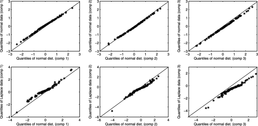
Figure 1: The Q–Q plots for the one-sample examples, where the specified distribution is trivariate normal. The plots in the first and the second rows are for the examples, where the distributions of the data are trivariate normal and trivariate Laplace, respectively.

It is clearly evident from the plots in the first row of Figure 1 that the specified distribution fits the data well as the points in those plots are tightly clustered around the straight line with slope $=1$ and intercept $=0$. On the other hand, in each Q–Q plot in the second row, the points are significantly deviating from the straight line with slope $=1$ and intercept $=0$, and the points are actually clustered around a nonlinear curve. We have also computed the $p$-values for the one-sample test discussed in Section 3 for testing $H_{0}\colon\ F=F_{0}$ against $H_{1}\colon\ F\neq F_{0}$ for these two simulated data sets. We have obtained a high $p$-value $=0.784$ for the first sample whereas the $p$-value for the second example is $0.049$, which is quite small.

We next consider two simulated data sets to demonstrate our Q–Q plots for the two-sample problem. In both the data sets, the distribution of the first sample $F$ was chosen to be the standard trivariate normal distribution while $G$, the distribution of the second sample, was taken to be the standard trivariate normal in one set and the trivariate Laplace distribution in the other set. The size of each sample was 100. The Q–Q plots for the two data sets are displayed in Figure 2. In each plot in the first row of Figure 2, the points are tightly clustered around the straight line with slope $=1$ and intercept $=0$. On the other hand, the points are significantly deviating from the straight line with slope $=1$ and intercept $=0$ in each plot in the second row of Figure 2. We also carried out the two-sample test described in Section 3 for testing $H_{0}^{*}\colon\ F=G$ against $H_{1}^{*}\colon\ F\neq G$, and we obtained a high $p$-value $=0.731$ for the first data set whereas a small $p$-value $=0.048$ was obtained for the second data set.

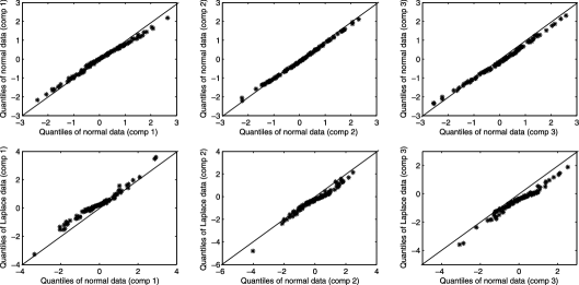
Figure 2: The Q–Q plots for the two-sample problem. The plots in the first row for an example, where the samples are generated from the same distribution, and those in the second row for an example, where the samples are generated from different distributions.

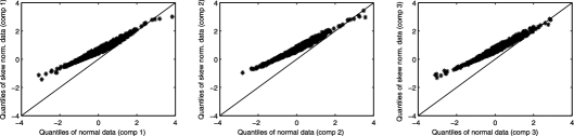
Figure 3: The Q–Q plots for the two-sample problem, where the first sample is generated from the standard trivariate normal distribution, and the second sample is generated from a trivariate skew-normal distribution.

4.1 Detection of special features using multivariate Q–Q plots

We now consider a two-sample problem, where the first sample consists of 100 i.i.d. observations from the standard trivariate normal distribution ($F$), and the second sample consists of 100 i.i.d. observations from a trivariate skew-normal distribution ($G$) (see Azzalini and Dalla Valle ([4], page 717)). The p.d.f. of the trivariate skew-normal distribution is given by $f({\mathbf{z}})=2\phi_{3}({\mathbf{z}};\Omega)\Phi(\alpha^{T}{\mathbf{z}})$, where ${\mathbf{z}}\in\mathbb{R}^{3}$, $\alpha^{T}=\frac{\lambda^{T}\Psi^{-1}\Delta^{-1}}{\sqrt{1+\lambda^{T}\Psi^{-1}\lambda}}$, $\Delta=\operatorname{diag}(\sqrt{1-\delta_{1}^{2}},\sqrt{1-\delta_{2}^{2}},\sqrt{1-\delta_{3}^{2}})$, $\lambda=(\frac{\delta_{1}}{\sqrt{1-\delta_{1}^{2}}},\frac{\delta_{2}}{\sqrt{1-\delta_{2}^{2}}},\frac{\delta_{3}}{\sqrt{1-\delta_{3}^{2}}})^{T}$, and $\Omega=\Delta(\Psi+\lambda\lambda^{T})\Delta$. Here $\phi_{3}({\mathbf{z}};\Omega)$ denotes the p.d.f. of a trivariate normal distribution with standardized marginals and correlation matrix $\Omega$, and $\Phi$ is the distribution function of the standard univariate normal distribution. In this study, we have considered $\delta_{1}=\delta_{2}=\delta_{3}=0.9$ and $\Psi=I_{d}$. The Q–Q plots for this two-sample problem are displayed in Figure 3, and we see a heavier tail in one direction in each plot in this figure. This is an indication that one sample is generated from a more skewed distribution than the other. Also, the small $p$-value $=0.048$ obtained using our two-sample test for testing $H_{0}^{*}\colon\ F=G$ against $H_{1}^{*}\colon\ F\neq G$ implies that the two distributions are significantly different in this data set.

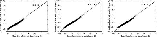
Figure 4: The Q–Q plots for the two-sample problem, where the first sample is generated from the standard trivariate normal distribution, and the second sample contains some outliers.

We next consider an example to demonstrate how our Q–Q plots can be used to detect outliers present in the data. We again consider a two-sample problem, where the first sample consists of 100 i.i.d. observations from the standard trivariate normal distribution. The second sample consists of 97 i.i.d. observations from the standard trivariate normal distribution and the remaining three data points in the sample are $(10,10,10)$, $(9,9,9)$ and $(8,8,8)$. The Q–Q plots for this data set are displayed in Figure 4. The presence of three outliers in the second sample is clearly indicated by the plots in Figure 4.

4.2 Analysis of real data

We first consider Fisher’s Iris data, which is available in http://archive.ics.uci.edu/ml. In this data, there are three multivariate samples corresponding to three different varieties of Iris, namely, Iris setosa, Iris virginica and Iris versicolor. Each sample has size 50. In each sample, there are four measurements, namely, the sepal length, the sepal width, the petal length and the petal width. We would like to determine how close is the distribution of each sample to a four-dimensional normal distribution. This can be formulated as a one-sample problem, where $F$ is the distribution of a sample, and the four-dimensional normal distribution is our specified distribution $F_{0}$. Note that $F_{0}$ involves an unknown mean $\bolds\mu$ and an unknown dispersion $\Sigma$. For each species, following the remarks after Theorem 2.1, we estimated $\bolds\mu$ and $\Sigma$ by the sample mean vector and the sample dispersion matrix, which are maximum likelihood estimates. Then we standardized the data in each sample using the corresponding sample mean vector and the corresponding sample dispersion matrix. The Q–Q plots in Figure 5 were constructed using the spatial quantiles of a standardized sample and the spatial quantiles of the standard four-dimensional normal distribution.

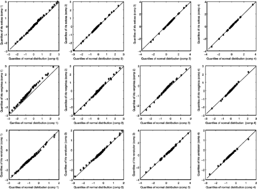
Figure 5: The Q–Q plots for Iris setosa (first row), Iris virginica (second row) and Iris versicolor (third row).

It is visible in the plots in Figure 5 that in almost all cases, the points are tightly clustered around the straight line with slope $=1$ and intercept $=0$ except in the first plot for Iris virginica, where the points deviate to some extent from that straight line. Our one-sample test for testing $H_{0}\colon\ F=F_{0}$ against $H_{1}\colon\ F\neq F_{0}$ led to very high $p$-values, namely, $0.841$, $0.413$ and $0.582$ for Iris setosa, Iris virginica and Iris versicolor, respectively. These $p$-values imply that $H_{0}$ is to be accepted, and multivariate normal distributions seem to fit the data well for all three Iris species.

Our next real data set is the Vertebral Column data, which is available in http://archive.ics.uci.edu/ml/datasets/Vertebral+Column. This data set contains six variables on 310 patients, who belong to two groups. Among the 310 patients, 100 are normal, and the remaining 210 of them are abnormal. We view it as a two-sample problem with $F$ as the distribution of the measurements corresponding to the normal patients, and $G$ as the distribution of the measurements corresponding to the abnormal patients. In this study, we considered only two variables, namely, the pelvic incidence and the pelvic tilt as these two pelvic parameters are strongly associated with the severity and the stiffness of lumbosacral spondylolisthesis. Both the pelvic incidence and the pelvic tilt are angles and measured in the same unit, and no standardization of the data is necessary in order to compute and compare the spatial quantiles of these two samples. In Figure 6, we display the Q–Q plots for this data. The points in the Q–Q plots are clearly not clustered around any straight line. In fact, most of the points in each plot lie on a stretched S-shaped curve, which indicates that the distribution $G$ associated with the abnormal patients has heavier tails than the distribution $F$ associated with the normal patients. The $p$-value obtained using the two-sample test for testing $H_{0}^{*}\colon\ F=G$ against $H_{1}^{*}\colon\ F\neq G$ is $0.038$, which also indicates that the two distributions are significantly different.

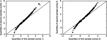
Figure 6: The Q–Q plots for the vertebral column data.

The third real data set that we consider is the Monthly Sunspot number data, which is available in http://www.ngdc.noaa.gov/stp/solar/ssndata.html. This data set contains monthly average number of sunspots during the period of 1749 to 2009. As data for 1749 and 2009 are incomplete, we have carried out our analysis on the observations for the remaining 259 (1750 to 2008) years. We divided the data into two samples. One sample contains six-dimensional data corresponding to the six months January, February, March, October, November and December, and the other one consists of six-dimensional data corresponding to the months April, May, June, July, August and September. The motivation behind splitting the data into two parts corresponding to the periods October–March and April–September comes from the fact that one equinox in a year occurs on March 20–21 and another on September 22–23. We treat this as a two-sample problem, where $F$ and $G$ are the distributions corresponding to the sunspot numbers during the periods October–March and April–September, respectively. The Q–Q plots for the data are presented in Figure 7. In each of the plots, the points lie very close to a straight line with slope $=2$ and intercept $=0$. In view of the remark after Theorem 2.2, these plots indicate that the distributions $F$ and $G$ are related by the equation $F({\mathbf{x}})=G({\mathbf{x}}/2)$. Hence, the two multivariate samples corresponding to the two periods October–March and April–September have distributions that differ only in the scales of the variables. The two distributions have the same location, and one distribution can be obtained from the other by a scale transformation using the scale factor $2$. This fact was further confirmed when we carried out some alternative statistical analysis of the data such as the comparison of the marginal quantiles and the direct comparison of the means and the variances of the variables.

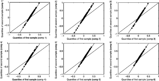
Figure 7: The Q–Q plots for the monthly sunspot number data.

4.3 Multivariate Q–Q plots for data with large dimensions

When the dimension of the data is large, there will be too many two-dimensional plots, and it will be inconvenient to display and visually examine all of them. In that case, one can plot $(l,Q_{{\cal{X}},l}({\mathbf{u}}_{k})-Q_{{\cal{Y}},l}({\mathbf{u}}_{k}))$ for $k=1,\ldots,(n+m)$ and $l=1,\ldots,d$ in a single two-dimensional plot with $d$ vertical lines parallel to one another. We next demonstrate this procedure on some simulated and real data sets.

First, we consider a two-sample problem, where the data in each sample consists of 10 i.i.d. observations from a standard Brownian motion with its mean function $m(t)=0$ and covariance kernel $k(s,t)=\min(s,t)$, where $s$, $t\in[0,1]$ (note that $F=G$ here). For our second data set, one sample consists of 10 i.i.d. observations from a standard Brownian motion with its mean function $m_{1}(t)=0$ and covariance kernel $k_{1}(s,t)=\min(s,t)$ as before (i.e., we have the same $F$ as before). However, the second sample in the second data consists of 10 i.i.d. observations from a Brownian motion with its mean function $m_{2}(t)=2$ and covariance kernel $k_{2}(s,t)=2\min(s,t)$ (which corresponds to the distribution $G$). In our study, we considered equally spaced points $t_{1},\ldots,t_{20}$ in $[0,1]$ and sampled the observations at those time points.

The fourth real data set that we consider is the Sea Level Pressures data, which is available in http://www.cpc.noaa.gov/data/indices/darwin and http://www.cpc.noaa.gov/data/indices/tahiti. This data set consists of monthly sea level pressures from two different islands in the southern Pacific ocean, namely, Darwin ($13^{\circ}$S, $131^{\circ}$E) and Tahiti ($17^{\circ}$S, $149^{\circ}$W) during the period 1850–2008. Thus, we have a two-sample problem with each sample corresponding to an island and containing 159 twelve-dimensional observations. Here $F$ and $G$ are the distributions of the multivariate observations corresponding to the two islands. For this data, each data point corresponds to a year, and each coordinate of a data point corresponds to an observation in a particular month.

The plots of the quantile differences for the above three data sets are displayed in Figure 8. In the first plot in Figure 8, the points in each vertical line are tightly clustered around a horizontal straight line passing through the origin, which indicates that the samples are obtained from similar distributions. It is further confirmed by the large $p$-value $=0.623$ obtained using our two-sample test for testing $H_{0}^{*}\colon\ F=G$ against $H_{1}^{*}\colon\ F\neq G$. On the other hand, the difference in the locations and the scales of the two distributions $F$ and $G$ are clearly visible in the second plot in Figure 8. The $p$-value obtained using our two-sample test in this case is $0.042$, which indicates significant difference between the two distributions and strong support in favour of $H_{1}^{*}\colon\ F\neq G$. It is also amply indicated by the third plot in Figure 8 as well as the small $p$-value $=0.045$ obtained using our two-sample test that the distributions $F$ and $G$ for the two samples corresponding to the two islands Darwin and Tahiti are significantly different.

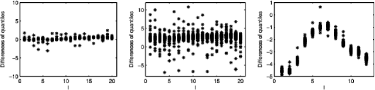
Figure 8: The quantile difference plots for the data on Brownian motions and sea level pressures.

5 Finite sample level and power study for different tests

Here we carry out some simulation studies to compare our tests with the well-known multivariate extensions of the Kolmogorov–Smirnov (KS) and the Cramer–von Mises (CVM) tests (see, e.g., Burke [8] and Justel, Peña and Zamar [20]) in the one-sample and the two-sample problems. For testing $H_{0}\colon\ F=F_{0}$ against $H_{1}\colon\ F\neq F_{0}$, the KS and the CVM test statistics are $T_{n}^{(1)}=\sup_{{\mathbf{x}}\in\mathbb{R}^{d}}\sqrt{n}|F_{n}({\mathbf{x}})-F_{0}({\mathbf{x}})|$ and $T_{n}^{(2)}=n\int_{{\mathbf{x}}\in\mathbb{R}^{d}}[F_{n}({\mathbf{x}})-F_{0}({\mathbf{x}})]^{2}\,\mathrm{d}F_{0}({\mathbf{x}})$, respectively, where $F_{n}({\mathbf{x}})$ is the empirical version of $F({\mathbf{x}})$. To test $H_{0}^{*}\colon\ F=G$ against $H_{1}^{*}\colon\ F\neq G$, the KS and the CVM test statistics are $T_{n,m}^{(1)}=\sup_{{\mathbf{x}}\in\mathbb{R}^{d}}\sqrt{n+m}|F_{n}({\mathbf{x}})-G_{m}({\mathbf{x}})|$ and $T_{n,m}^{(2)}=(n+m)\int_{{\mathbf{x}}\in\mathbb{R}^{d}}[F_{n}({\mathbf{x}})-G_{m}({\mathbf{x}})]^{2}\,\mathrm{d}M_{(n,m)}({\mathbf{x}})$, respectively, where $(n+m)M_{(n,m)}({\mathbf{x}})=nF_{n}({\mathbf{x}})+mG_{m}({\mathbf{x}})$, and $F_{n}$ and $G_{m}$ are the empirical versions of $F$ and $G$, respectively. The KS and the CVM tests for multivariate data can be implemented using the asymptotic distributions of the corresponding test statistics.

For the one-sample problem, we have considered $F_{0}=N_{d}$ and $F=(1-\beta)N_{d}+\beta C_{d}$ and $(1-\beta)N_{d}+\beta L_{d}$. Here $\beta\in[0,1]$, $N_{d}$, $L_{d}$ and $C_{d}$ are the $d$-dimensional standard normal distribution, the $d$-dimensional Laplace distribution with p.d.f. $f({\mathbf{x}})=(\Gamma(d/2)/2\Gamma(d)\pi^{d/2})\exp^{-\|{\mathbf{x}}\|}$ and the $d$-dimensional Cauchy distribution with p.d.f. $f({\mathbf{x}})=(\Gamma((d+1)/2)/\sqrt{\pi}\Gamma(d/2))(1+\|{\mathbf{x}}\|^{2})^{-(d+1)/2}$, respectively. In the case of the two-sample problem, we have considered $F=N_{d}$ and $G=(1-\beta)N_{d}+\beta C_{d}$ and $(1-\beta)N_{d}+\beta L_{d}$.

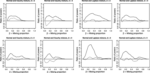
Figure 9: The graphs of the ratios of empirical powers based on 1000 Monte Carlo replications at $5\%$ nominal level. The numerator in each ratio is the power of our test while the denominators of the ratios corresponding to the solid and the dotted curves are the powers of the KS and the CVM tests, respectively. The first row corresponds to the one-sample problem with $n=10$, and the second row corresponds to the two-sample problem with $n=m=10$.

In Figure 9, we have plotted the ratio between the empirical power of our test (numerator) and that of another test (denominator) for different values of the parameter $\beta$. It is evident from Figure 9 that our test is significantly more powerful than the KS test in all the cases considered in our simulation study. However, the CVM test performs better than our test in some cases, and our test outperforms the CVM test in some other cases.

Friedman and Rafsky [15] proposed a multivariate generalization of the Wald–Wolfowitz run test using the idea of minimum spanning tree (the MST-run test). We have compared the empirical powers of our two-sample test with those of the MST-run test for $F=N_{d}({\mathbf{0}},I_{d})$ and $G=N_{d}(d^{-1/2}\Delta{\mathbf{1}}_{d},\sigma I_{d})$, where $N_{d}(\bolds\mu,\Sigma)$ is the $d$-dimensional normal distribution with mean $\bolds\mu$ and dispersion $\Sigma$, ${\mathbf{1}}_{d}$ is the $d$-dimensional vector of $1$’s, and the values of $\Delta$ and $\sigma$ are chosen as in Friedman and Rafsky ([16], page 706). For sample sizes $n=m=100$ and $5\%$ nominal level, the results are reported in Table 1, and it is clear that the MST-run test has inferior performance compared to our test.

Table 1: Comparison of the empirical powers based on 100 Monte Carlo replications of our two-sample test and the MST-run test in different dimensions

	$d=2$	$d=5$	$d=10$	$d=20$
	$\Delta=0.5,\sigma=1$	$\Delta=0.75,\sigma=1$	$\Delta=1.0,\sigma=1$	$\Delta=1.2,\sigma=1$
Our test	$0.55$	$0.70$	$0.83$	$0.99$
MST-run test	$0.35$	$0.64$	$0.78$	$0.86$
	$\Delta=0,\sigma=1.2$	$\Delta=0,\sigma=1.2$	$\Delta=0,\sigma=1.1$	$\Delta=0,\sigma=1.075$
Our test	$0.17$	$0.26$	$0.07$	$0.14$
MST-run test	$0.14$	$0.21$	$0.09$	$0.13$

For univariate data, our proposed tests in the one-sample and the two-sample problems lead to new tests that have previously not been considered in the literature. In addition to the KS and the CVM tests, there are several other tests that are available in the literature (see, e.g., Shapiro and Wilk [33], Anderson and Darling [3] and Ahmad [1, 2]) for comparing the distributions of univariate data in the one-sample and the two-sample problems. We have discussed and compared the performance of these tests for univariate data in detail in the supplemental article (see Dhar, Chakraborty and Chaudhuri [11]).

6 Asymptotic power study under contiguous alternatives

Since our tests, the KS and the CVM tests are all asymptotically consistent, a natural question is how the asymptotic powers of our tests and the KS and the CVM tests compare with one another under contiguous alternatives (see Hájek and Šidák [19]). In the case of the one-sample problem, the null hypothesis is given by $H_{0}\colon\ F({\mathbf{x}})=F_{0}({\mathbf{x}})$, and we consider a sequence of contiguous alternatives $H_{n}\colon\ F({\mathbf{x}})=(1-\gamma/\sqrt{n})F_{0}({\mathbf{x}})+(\gamma/\sqrt{n})H({\mathbf{x}})$ for a fixed $\gamma>0$ and $n=1,2,\ldots\,$. Consider a multivariate Gaussian process $Z_{1}^{\prime}({\mathbf{u}})$ with the mean function

$$m_{1}({\mathbf{u}})=\gamma\bigl{[}D_{1}\bigl{\{}Q_{F_{0}}({\mathbf{u}})\bigr{\}}\bigr{]}^{-1}E_{H}\biggl{\{}\frac{{\mathbf{x}}-Q_{F_{0}}({\mathbf{u}})}{\|{\mathbf{x}}-Q_{F_{0}}({\mathbf{u}})\|}+{\mathbf{u}}\biggr{\}}$$

and the covariance kernel $k_{1}({\mathbf{u}}_{1},{\mathbf{u}}_{2})$, where $k_{1}({\mathbf{u}}_{1},{\mathbf{u}}_{2})$ is as defined before Theorem 3.1. Let ${\cal{V}}^{\prime}=\int\|Z_{1}^{\prime}({\mathbf{u}})\|^{2}\,\mathrm{d}{\mathbf{u}}$, where the integral is over the same closed ball as in the definition of $V_{n}$ in Section 3. We now state a theorem describing the asymptotic powers of the test based on $V_{n}$ as well as the KS and the CVM tests under contiguous alternatives.

Theorem 6.1

Assume that $F_{0}$ and $H$ have continuous and positive densities $f_{0}$ and $h$, respectively, on $\mathbb{R}^{d}(d\geq 2)$, and $E_{F_{0}}\{\frac{h({\mathbf{x}})}{f_{0}({\mathbf{x}})}-1\}^{2}<\infty$. Then, the sequence of alternatives $H_{n}$ form a contiguous sequence. Under such alternatives, the asymptotic power of the test based on $V_{n}$ is given by $P_{\gamma}[{\cal{V}}^{\prime}>c_{1}(\alpha)]$, where $c_{1}(\alpha)$ is as defined in Theorem 3.1 such that $P_{\gamma=0}[{\cal{V}}^{\prime}>c_{1}(\alpha)]=\alpha$. Further, under those alternatives, the asymptotic powers of the tests based on $T_{n}^{(1)}$ and $T_{n}^{(2)}$ are given by $P_{\gamma}[\sup_{{\mathbf{t}\in\mathbb{R}^{d}}}|Z_{1}^{\prime\prime}({\mathbf{t}})|>c_{1}^{*}(\alpha)]$ and $P_{\gamma}[\int_{{\mathbf{t}}\in\mathbb{R}^{d}}\{Z_{1}^{\prime\prime}({\mathbf{t}})\}^{2}\,\mathrm{d}F_{0}({\mathbf{t}})>c_{1}^{**}(\alpha)]$, respectively, where $Z_{1}^{\prime\prime}({\mathbf{t}})$ $({\mathbf{t}}\in\mathbb{R}^{d})$ is a Gaussian process with its mean function $m_{1}^{\prime}({\mathbf{t}})=\gamma\{H({\mathbf{t}})-F_{0}({\mathbf{t}})\}$ and covariance kernel $k_{3}({\mathbf{t}}_{1},{\mathbf{t}}_{2})=F_{0}(\min({\mathbf{t}}_{1},{\mathbf{t}}_{2}))-F_{0}({\mathbf{t}}_{1})F_{0}({\mathbf{t}}_{2})$. Here “$\min$” denotes the coordinatewise minimum of the two vectors in $\mathbb{R}^{d}$, and $c_{1}^{*}(\alpha)$ and $c_{1}^{**}(\alpha)$ satisfy $P_{\gamma=0}[\sup_{{\mathbf{t}}\in\mathbb{R}^{d}}|Z_{1}^{\prime\prime}({\mathbf{t}})|>c_{1}^{*}(\alpha)]=\alpha$ and $P_{\gamma=0}[\int_{{\mathbf{t}}\in\mathbb{R}^{d}}\{Z_{1}^{\prime\prime}({\mathbf{t}})\}^{2}\,\mathrm{d}F_{0}({\mathbf{t}})>c_{1}^{**}(\alpha)]=\alpha$.

Next, for the two-sample problem, the null hypothesis is given by $H_{0}^{*}\colon\ F({\mathbf{x}})=G({\mathbf{x}})$, and we consider a sequence of alternatives $H_{n,m}^{*}\colon\ G({\mathbf{x}})=(1-\gamma/\sqrt{n+m})F({\mathbf{x}})+(\gamma/\sqrt{n+m})H({\mathbf{x}})$ for a fixed $\gamma>0$ and $n,m=1,2,\ldots\,$. Consider a multivariate Gaussian process $Z_{2}^{\prime}({\mathbf{u}})$ with the mean function

$$m_{2}({\mathbf{u}})=-\gamma\bigl{[}D_{1}\bigl{(}Q_{F}({\mathbf{u}})\bigr{)}\bigr{]}^{-1}E_{H}\biggl{\{}\frac{{\mathbf{y}}-Q_{F}({\mathbf{u}})}{\|{\mathbf{y}}-Q_{F}({\mathbf{u}})\|}+{\mathbf{u}}\biggr{\}}$$

and the covariance kernel $k_{2}({\mathbf{u}}_{1},{\mathbf{u}}_{2})$. Here $k_{2}({\mathbf{u}}_{1},{\mathbf{u}}_{2})$ is as defined before Theorem 3.2. Let ${\cal{T}}^{\prime}=\int\|Z_{2}^{\prime}({\mathbf{u}})\|^{2}\,\mathrm{d}{\mathbf{u}}$, where the integral is over the same closed ball as in the definition of $T_{n,m}$ in Section 3. We now state a theorem describing the asymptotic powers of the test based on $T_{n,m}$ as well as the KS and the CVM tests under contiguous alternatives.

Theorem 6.2

Assume that $F$ and $H$ have continuous and positive densities $f$ and $h$, respectively, on $\mathbb{R}^{d}$ $(d\geq 2)$, $E_{F}\{\frac{h({\mathbf{y}})}{f({\mathbf{y}})}-1\}^{2}<\infty$, and $n,m\rightarrow\infty$ in such a way that $\lim_{n,m\rightarrow\infty}\frac{n}{(n+m)}=\lambda\in(0,1)$. Then, the sequence of densities associated with alternatives $H_{n,m}^{*}$ form a contiguous sequence. Under such alternatives, the asymptotic power of the test based on $T_{n,m}$ is given by $P_{\gamma}[{\cal{T}}^{\prime}>c_{2}(\alpha)]$, where $c_{2}(\alpha)$ is as defined in Theorem 3.2 such that $P_{\gamma=0}[{\cal{T}}^{\prime}>c_{2}(\alpha)]=\alpha$. Further, under those alternatives, the asymptotic powers of the tests based on $T_{n,m}^{(1)}$ and $T_{n,m}^{(2)}$ are given by $P_{\gamma}[\sup_{{\mathbf{t}}\in\mathbb{R}^{d}}|Z_{2}^{\prime\prime}({\mathbf{t}})|>c_{2}^{*}(\alpha)]$ and $P_{\gamma}[\int_{{\mathbf{t}}\in\mathbb{R}^{d}}\{Z_{2}^{\prime\prime}({\mathbf{t}})\}^{2}\,\mathrm{d}F({\mathbf{t}})>c_{2}^{**}(\alpha)]$, respectively, where $Z_{2}^{\prime\prime}({\mathbf{t}})$ $({\mathbf{t}}\in\mathbb{R}^{d})$ is a Gaussian process with its mean function $m_{2}^{\prime}({\mathbf{t}})=-\gamma\{H({\mathbf{t}})-F({\mathbf{t}})\}$ and covariance kernel $k_{4}({\mathbf{t}}_{1},{\mathbf{t}}_{2})=\frac{F(\min({\mathbf{t}}_{1},{\mathbf{t}}_{2}))-F({\mathbf{t}}_{1})F({\mathbf{t}}_{2})}{\lambda(1-\lambda)}$. Here also “$\min$” denotes the coordinatewise minimum of the two vectors in $\mathbb{R}^{d}$, and $c_{2}^{*}(\alpha)$ and $c_{2}^{**}(\alpha)$ are such that $P_{\gamma=0}[\sup_{{\mathbf{t}}\in\mathbb{R}^{d}}|Z_{2}^{\prime\prime}({\mathbf{t}})|>c_{2}^{*}(\alpha)]=\alpha$ and $P_{\gamma=0}[\int_{{\mathbf{t}}\in\mathbb{R}^{d}}\{Z_{2}^{\prime\prime}({\mathbf{t}})\}^{2}\,\mathrm{d}F({\mathbf{t}})>c_{2}^{**}(\alpha)]=\alpha$.

Theorems 6.1 and 6.2 enable us to derive the Pitman efficacies of our tests relative to the KS and the CVM tests. The Pitman efficacy (see, e.g., Serfling [31] and Lehmann and Romano [25]) of our test relative to another test for varying choices of the asymptotic power (determined by $\gamma$) is given by $(\gamma^{\prime}/\gamma)^{2}$, where $\gamma$ and $\gamma^{\prime}$ are such that the asymptotic power of our test under contiguous alternatives $(1-\gamma/\sqrt{n})F_{0}({\mathbf{x}})+(\gamma/\sqrt{n})H({\mathbf{x}})$ (or $(1-\gamma/\sqrt{n+m})F({\mathbf{x}})+(\gamma/\sqrt{n+m})H({\mathbf{x}})$) is the same as the asymptotic power of the other test under contiguous alternatives $(1-\gamma^{\prime}/\sqrt{n})F_{0}({\mathbf{x}})+(\gamma^{\prime}/\sqrt{n})H({\mathbf{x}})$ (or $(1-\gamma^{\prime}/\sqrt{n+m})F({\mathbf{x}})+(\gamma^{\prime}/\sqrt{n+m})H({\mathbf{x}})$).

In order to compute the critical values and the powers of our one-sample and two-sample tests, we have used 1000 simulations of each Gaussian process and approximated the integral of the squared norm of a multivariate Gaussian process by the average of the squared norms of some appropriate multivariate normal random vectors. In this numerical study, we could compute the true covariance matrices as the underlying distributions were known. We have computed the critical value and the asymptotic power of the CVM test in a similar way. However, in the case of the KS test, we have approximated the supremum of a Gaussian process by a maximum over 1000 simulations of the process.

Figure 10: The Pitman efficacy of our test relative to the KS test (solid curve) and the CVM test (dotted curve) at $5\%$ nominal level. The first row corresponds to the one-sample problem, and the second row corresponds to the two-sample problem.

In Figure 10, we have plotted the Pitman efficacy of our test for different values of the asymptotic power. It is clearly indicated by Figure 10 that our test and the CVM test outperform the KS test in terms of the Pitman efficacy in all the cases considered here. However, between our test and the CVM test, one has superior performance in some cases while the other has superior performance in some other cases, and there is only a small difference in their performance.

Appendix: Proofs

Proof of Theorem 2.1 In view of the results in Chaudhuri [10] and Koltchinskii [24], we have

$$\sup_{{\mathbf{u}}}\bigl{\|}Q_{{\cal{X}}}({\mathbf{u}})-Q_{F}({\mathbf{u}})\bigr{\|}=\mathrm{o}_{P}(1),$$ (1)

where the supremum is taken over any given closed ball with the center at the origin and the radius strictly smaller than one. When $F=F_{0}$, we have $Q_{F}({\mathbf{u}})=Q_{F_{0}}({\mathbf{u}})$ for all $\|{\mathbf{u}}\|<1$. This along with the uniform convergence result in (1) leads to the proof of the “if part” of the theorem.

Next, consider some ${\mathbf{u}}$ with $\|{\mathbf{u}}\|<1$. It follows from the conditions in the theorem that with probability tending to one, the spatial rank vectors ${\mathbf{u}}_{k}$’s form a dense subset of the unit ball around the origin as $n\rightarrow\infty$. Since

$$\lim_{n\rightarrow\infty}P\Biggl{(}\bigcap_{i=1}^{d}\bigl{[}S_{n,i}({\cal{X}},F_{0})\subseteq L(\varepsilon)\bigr{]}\Biggr{)}=1$$

for every $\varepsilon>0$, we must have $Q_{F}({\mathbf{u}})=Q_{F_{0}}({\mathbf{u}})$ in view of (1). It now follows from the characterization of multivariate distributions by the spatial quantiles (see Corollary 2.9 in Koltchinskii ([24], page 446)) that $F=F_{0}$. This completes the proof of the “only if part” of the theorem.

Proof of Theorem 2.2 It follows from the results in Chaudhuri [10] and Koltchinskii [24] that for the two independent samples ${\cal{X}}$ and ${\cal{Y}}$, we have $\sup_{{\mathbf{u}}}\|(Q_{{\cal{X}}}({\mathbf{u}}),Q_{{\cal{Y}}}({\mathbf{u}}))-(Q_{F}({\mathbf{u}}),Q_{G}({\mathbf{u}}))\|=\mathrm{o}_{P}(1)$ when $n$, $m\rightarrow\infty$ in such a way that $\lim_{n,m\rightarrow\infty}\frac{n}{(n+m)}=\lambda\in(0,1)$. Here the supremum is taken over any given closed ball with the center at the origin and the radius strictly smaller than one. Then the proof of the theorem follows by similar arguments as in the proof of Theorem 2.1.

Proof of Theorem 3.1 As proved in Koltchinskii [24], the centered and normalized stochastic process $\sqrt{n}\{Q_{{\cal{X}}}({\mathbf{u}})-Q_{F_{0}}({\mathbf{u}})\}$ converges weakly to the Gaussian process $Z_{1}({\mathbf{u}})$ (defined in Section 3) under $H_{0}$. Here ${\mathbf{u}}$ lies in any given closed ball with the center at the origin and the radius strictly smaller than one. It follows from the continuity of the integral functional that $V_{n}$ converges in distribution to ${\cal{V}}$. Consequently, the asymptotic level of the test will be $\alpha$.

The asymptotic power of the test is given by $\lim_{n\rightarrow\infty}P_{H_{1}}[V_{n}>c_{1}(\alpha)]$. Now, note that $V_{n}>c_{1}(\alpha)$ if and only if $n\int\|\{Q_{{\cal{X}}}({\mathbf{u}})-Q_{F_{0}}({\mathbf{u}})\}-\{Q_{F}({\mathbf{u}})-Q_{F_{0}}({\mathbf{u}})\}\|^{2}\,\mathrm{d}{\mathbf{u}}>c_{1}(\alpha)+n[\int\langle\{Q_{F}({\mathbf{u}})-Q_{F_{0}}({\mathbf{u}})\},\{Q_{F}({\mathbf{u}})-Q_{F_{0}}({\mathbf{u}})\}\rangle\,\mathrm{d}{\mathbf{u}}-2\int\langle\{Q_{{\cal{X}}}({\mathbf{u}})-Q_{F_{0}}({\mathbf{u}})\},\{Q_{F}({\mathbf{u}})-Q_{F_{0}}({\mathbf{u}})\}\rangle\,\mathrm{d}{\mathbf{u}}]$. Here the integrals are over a closed ball with the center at the origin and the radius strictly smaller than one as before.

When $F\neq F_{0}$, in view of the characterization property of the spatial quantiles (see Corollary 2.9 in Koltchinskii [24]), we have $Q_{F}({\mathbf{u}})\neq Q_{F_{0}}({\mathbf{u}})$ for some ${\mathbf{u}}$ with $\|{\mathbf{u}}\|<1$. The uniform convergence of $Q_{{\cal{X}}}({\mathbf{u}})$ to $Q_{F}({\mathbf{u}})$ and the continuity of the spatial quantiles $Q_{F}({\mathbf{u}})$ and $Q_{F_{0}}({\mathbf{u}})$ as functions of ${\mathbf{u}}$ imply that $c_{1}(\alpha)+n[\int\langle\{Q_{F}({\mathbf{u}})-Q_{F_{0}}({\mathbf{u}})\},\{Q_{F}({\mathbf{u}})-Q_{F_{0}}({\mathbf{u}})\}\rangle\,\mathrm{d}{\mathbf{u}}-2\int\langle\{Q_{{\cal{X}}}({\mathbf{u}})-Q_{F_{0}}({\mathbf{u}})\},\{Q_{F}({\mathbf{u}})-Q_{F_{0}}({\mathbf{u}})\}\rangle\,\mathrm{d}{\mathbf{u}}]$ tends to $-\infty$ in probability as $n\rightarrow\infty$. Hence, $P_{H_{1}}[V_{n}>c_{1}(\alpha)]\rightarrow 1$ as $n\rightarrow\infty$. This completes the proof.

Proof of Theorem 3.2 Arguing in a similar way as in the proof of Theorem 3.1 and using the weak convergence results in Koltchinskii [24], and the independence of the two samples, if $n,m\rightarrow\infty$ in such a way that $\lambda=\lim_{n,m\rightarrow\infty}\frac{n}{(n+m)}\in(0,1)$, one can show that $T_{n,m}$ converges in distribution to ${\cal{T}}$ under $H_{0}^{*}$, and consequently, the asymptotic level of the test that rejects $H_{0}^{*}$ when $T_{n,m}>c_{2}(\alpha)$ will be $\alpha$. Next, the asymptotic power of the test is given by $P_{H_{1}^{*}}[T_{n,m}>c_{2}(\alpha)]$. Using similar arguments as in the second part of the proof of Theorem 3.1, one can establish that $P_{H_{1}^{*}}[T_{n,m}>c_{2}(\alpha)]\rightarrow 1$ as $n,m\rightarrow\infty$.

Proof of Theorem 6.1 The logarithm of the likelihood ratio for testing $H_{0}$ against $H_{n}$ is

$$L_{n} = \sum_{i=1}^{n}\log\frac{(1-\gamma/\sqrt{n})f_{0}({\mathbf{x}}_{i})+(\gamma/\sqrt{n})h({\mathbf{x}}_{i})}{f_{0}({\mathbf{x}}_{i})}=\sum_{i=1}^{n}\log\biggl{[}1+(\gamma/\sqrt{n})\biggl{\{}\frac{h({\mathbf{x}}_{i})}{f_{0}({\mathbf{x}}_{i})}-1\biggr{\}}\biggr{]}$$

$$= \frac{\gamma}{\sqrt{n}}\sum_{i=1}^{n}\biggl{\{}\frac{h({\mathbf{x}}_{i})}{f_{0}({\mathbf{x}}_{i})}-1\biggr{\}}-\frac{\gamma^{2}}{2n}\sum_{i=1}^{n}\biggl{\{}\frac{h({\mathbf{x}}_{i})}{f_{0}({\mathbf{x}}_{i})}-1\biggr{\}}^{2}+R_{n}$$

$$= \frac{\gamma}{\sqrt{n}}\sum_{i=1}^{n}k_{i}-\frac{\gamma^{2}}{2}\times\frac{1}{n}\sum_{i=1}^{n}k^{2}_{i}+R_{n},$$

where $k_{i}=\frac{h({\mathbf{x}}_{i})}{f_{0}({\mathbf{x}}_{i})}-1$. Note that $R_{n}\stackrel{{\scriptstyle P}}{{\rightarrow}}0$ as $n\rightarrow\infty$ since $\sigma^{2}:=E_{F_{0}}[\frac{h({\mathbf{x}})}{f_{0}({\mathbf{x}})}-1]^{2}<\infty$. Further, by a straightforward application of the central limit theorem, the first term in (Appendix: Proofs) is asymptotically normal with its mean $=0$ and variance $=\gamma^{2}\sigma^{2}$, and the second term in (Appendix: Proofs) converges in probability to $\frac{\gamma^{2}}{2}\sigma^{2}$ by the weak law of large numbers. So, using Slutsky’s theorem, $L_{n}$ is asymptotically normal with mean $=-\frac{\gamma^{2}}{2}\sigma^{2}$ and variance $=\gamma^{2}\sigma^{2}$. This ensures the contiguity of the sequence $H_{n}$ using the corollary to Lecam’s first lemma in Hájek and Šidák ([19], pages 204).

Now, we consider ${\mathbf{u}}_{1},\ldots,{\mathbf{u}}_{k}$ in a given closed ball with the center at the origin and the radius strictly smaller than one, and ${\mathbf{t}}_{1},\ldots,{\mathbf{t}}_{l}\in\mathbb{R}^{d}$. Then, under $H_{0}$, one can establish that the joint distribution of $\sqrt{n}\{Q_{{\cal{X}}}({\mathbf{u}}_{1})-Q_{F_{0}}({\mathbf{u}}_{1}),\ldots,Q_{{\cal{X}}}({\mathbf{u}}_{k})-Q_{F_{0}}({\mathbf{u}}_{k}),F_{n}({\mathbf{t}}_{1})-F_{0}({\mathbf{t}}_{1}),\ldots,F_{n}({\mathbf{t}}_{l})-F_{0}({\mathbf{t}}_{l}),L_{n}/\sqrt{n}\}$ is asymptotically multivariate normal. This follows using the Bahadur type linear expansion of $\{Q_{{\cal{X}}}({\mathbf{u}})-Q_{F_{0}}({\mathbf{u}})\}$ (see Chaudhuri [10]), the expansion of $L_{n}$ (see (Appendix: Proofs) above) and the fact that $F_{n}({\mathbf{t}})-F_{0}({\mathbf{t}})$ is a simple average of i.i.d. random variables. Note that for any $p=1,\ldots,k$, the covariance between $\sqrt{n}\{Q_{{\cal{X}}}({\mathbf{u}}_{p})-Q_{F_{0}}({\mathbf{u}}_{p})\}$ and $L_{n}$ is

$$\frac{\gamma}{n}E_{F_{0}}\Biggl{[}\sum_{i=1}^{n}\biggl{\{}D_{1}\bigl{[}Q_{F_{0}}({\mathbf{u}}_{p})\bigr{]}^{-1}\biggl{\{}\frac{{\mathbf{x}}_{i}-Q_{F_{0}}({\mathbf{u}}_{p})}{\|{\mathbf{x}}_{i}-Q_{F_{0}}({\mathbf{u}}_{p})\|}+{\mathbf{u}}_{p}\biggr{\}}\biggr{\}}\times\biggl{\{}\frac{h({\mathbf{x}}_{i})}{f_{0}({\mathbf{x}}_{i})}-1\biggr{\}}\Biggr{]}$$

$$\quad=\gamma\bigl{[}D_{1}\bigl{\{}Q_{F_{0}}({\mathbf{u}}_{p})\bigr{\}}\bigr{]}^{-1}E_{H}\biggl{\{}\frac{{\mathbf{x}}-Q_{F_{0}}({\mathbf{u}}_{p})}{\|{\mathbf{x}}-Q_{F_{0}}({\mathbf{u}}_{p})\|}+{\mathbf{u}}_{p}\biggr{\}}=m_{1}({\mathbf{u}}_{p}),$$

because $E_{F_{0}}\{\frac{{\mathbf{x}}-Q_{F_{0}}({\mathbf{u}}_{p})}{\|{\mathbf{x}}-Q_{F_{0}}({\mathbf{u}}_{p})\|}+{\mathbf{u}}_{p}\}={\mathbf{0}}$. Also, one can show that for any $j=1,\ldots,l$, the covariance between $\sqrt{n}\{F_{n}({\mathbf{t}}_{j})-F_{0}({\mathbf{t}}_{j})\}$ and $L_{n}$ is $m_{1}^{\prime}({\mathbf{t}}_{j})=\gamma\{H({\mathbf{t}}_{j})-F_{0}({\mathbf{t}}_{j})\}$.

Now, by a straightforward application of Lecam’s third lemma (see Hájek and Šidák [19], page 208), one can establish that under contiguous alternatives, $\sqrt{n}\{Q_{{\cal{X}}}({\mathbf{u}}_{1})-Q_{F_{0}}({\mathbf{u}}_{1}),\ldots,Q_{{\cal{X}}}({\mathbf{u}}_{k})-Q_{F_{0}}({\mathbf{u}}_{k})\}$ is asymptotically $kd$-dimensional multivariate normal with the mean vector having the $d$-dimensional $p$th block $m_{1}({\mathbf{u}}_{p})$ ($p=1,2,\ldots,k$), and its $kd\times kd$-dimensional covariance matrix is obtained from the covariance kernel $k_{1}$, which is given before Theorem 3.1. Further, the spatial quantile process satisfies the tightness condition under contiguous alternatives in view of the fact that it is tight under $H_{0}$. The tightness under $H_{0}$ follows from the weak convergence of the spatial quantile process (see Koltchinskii [24]). So, the spatial quantile process $\sqrt{n}\{Q_{{\cal{X}}}({\mathbf{u}})-Q_{F_{0}}({\mathbf{u}})\}$ converges to $Z_{1}^{\prime}({\mathbf{u}})$ under $H_{n}$, where $Z_{1}^{\prime}({\mathbf{u}})$ is a Gaussian process with its mean function $m_{1}({\mathbf{u}})$ and covariance kernel $k_{1}({\mathbf{u}}_{1},{\mathbf{u}}_{2})$. Hence, under $H_{n}$, the asymptotic power of the test based on $V_{n}$ is $P_{\gamma}[{\cal{V}}^{\prime}>c_{1}(\alpha)]$.

Similarly, using the weak convergence of the stochastic process $\sqrt{n}\{F_{n}({\mathbf{t}})-F({\mathbf{t}})\}$ under $H_{0}$ to a Gaussian process (see, e.g., Bickel and Wichura [6]) together with Lecam’s third lemma, one can show that under contiguous alternatives, $\sqrt{n}\{F_{n}({\mathbf{t}}_{1})-F_{0}({\mathbf{t}}_{1}),\ldots,F_{n}({\mathbf{t}}_{l})-F_{0}({\mathbf{t}}_{l})\}$ is asymptotically $l$-dimensional multivariate normal with the mean vector having the $j$th component $m_{1}^{\prime}({\mathbf{t}}_{j})$ ($j=1,\ldots,l$), and its $l\times l$-dimensional covariance matrix is obtained from the covariance kernel $k_{3}$, which is given in the statement of the theorem. Now, it follows from the finite-dimensional asymptotic distribution and the tightness of the process $\sqrt{n}\{F_{n}({\mathbf{t}})-F_{0}({\mathbf{t}})\}$ under contiguous alternatives that the stochastic process $\sqrt{n}\{F_{n}({\mathbf{t}})-F_{0}({\mathbf{t}})\}$ converges to $Z_{1}^{\prime\prime}({\mathbf{t}})$ under $H_{n}$, where $Z_{1}^{\prime\prime}({\mathbf{t}})$ is a Gaussian process with its mean function $m_{1}^{\prime}({\mathbf{t}})$ and covariance kernel $k_{3}({\mathbf{t}}_{1},{\mathbf{t}}_{2})$. Consequently, under $H_{n}$, the asymptotic powers of the tests based on $T_{n}^{(1)}$ and $T_{n}^{(2)}$ are $P_{\gamma}[\sup_{{\mathbf{t}}\in\mathbb{R}^{d}}|Z_{1}^{\prime\prime}({\mathbf{t}})|>c_{1}^{*}(\alpha)]$ and $P_{\gamma}[\int_{{\mathbf{t}}\in\mathbb{R}^{d}}\{Z_{1}^{\prime\prime}({\mathbf{t}})\}^{2}\,\mathrm{d}F_{0}({\mathbf{t}})>c_{1}^{**}(\alpha)]$, respectively.

Proof of Theorem 6.2 The logarithm of the likelihood ratio for testing $H_{0}^{*}$ against $H_{n,m}^{*}$ is

$$L_{n,m} = \log\frac{\prod_{i=1}^{n}f({\mathbf{x}}_{i})\prod_{j=1}^{m}\{(1-\gamma/\sqrt{n+m})f({\mathbf{y}}_{j})+\gamma/\sqrt{n+m}h({\mathbf{y}}_{j})\}}{\prod_{i=1}^{n}f({\mathbf{x}}_{i})\prod_{j=1}^{m}f({\mathbf{y}}_{j})}$$

$$= \sum_{j=1}^{m}\log\biggl{\{}1+\frac{\gamma}{\sqrt{n+m}}\biggl{(}\frac{h({\mathbf{y}}_{j})}{f({\mathbf{y}}_{j})}-1\biggr{)}\biggr{\}}$$

$$= \frac{\gamma}{\sqrt{n+m}}\sum_{j=1}^{m}k^{\prime}_{j}-\frac{\gamma^{2}}{2(n+m)}\times\sum_{j=1}^{m}k^{\prime 2}_{j}+R_{n,m},$$

where $k^{\prime}_{j}=\frac{h({\mathbf{y}}_{j})}{f({\mathbf{y}}_{j})}-1$. Note that $R_{n,m}\stackrel{{\scriptstyle P}}{{\rightarrow}}0$ as $n,m\rightarrow\infty$ since $\sigma_{*}^{2}:=E_{F}\{\frac{h({\mathbf{y}})}{f({\mathbf{y}})}-1\}^{2}<\infty$. Using similar arguments as in the proof of Theorem 6.1, $L_{n,m}$ is asymptotically normal with mean $=-\frac{\gamma^{2}}{2}(1-\lambda)\sigma_{*}^{2}$ and variance $=\gamma^{2}(1-\lambda)\sigma_{*}^{2}$. This fact ensures the contiguity of the sequence of densities under $H_{n,m}^{*}$ using the corollary to Lecam’s first lemma in Hájek and Šidák ([19], page 204).

Now, here also, we consider ${\mathbf{u}}_{1},\ldots,{\mathbf{u}}_{k}$ in a given closed ball with the center at the origin and the radius strictly smaller than one, and ${\mathbf{t}}_{1},\ldots,{\mathbf{t}}_{l}\in\mathbb{R}^{d}$. Then, under $H_{0}$, one can establish that the joint distribution of $\sqrt{n+m}\{Q_{{\cal{X}}}({\mathbf{u}}_{1})-Q_{{\cal{Y}}}({\mathbf{u}}_{1}),\ldots,Q_{{\cal{X}}}({\mathbf{u}}_{k})-Q_{{\cal{Y}}}({\mathbf{u}}_{k}),F_{n}({\mathbf{t}}_{1})-G_{m}({\mathbf{t}}_{1}),\ldots,F_{n}({\mathbf{t}}_{l})-G_{m}({\mathbf{t}}_{l}),L_{n,m}/\sqrt{n+m}\}$ is asymptotically multivariate normal. This asymptotic normality is a consequence of the independence of the two samples, the Bahadur type linear expansion of the difference of the spatial quantiles $Q_{{\cal{X}}}({\mathbf{u}})-Q_{{\cal{Y}}}({\mathbf{u}})$ (see Chaudhuri [10]), the expansion of $L_{n,m}$ given in (Appendix: Proofs) and the fact that $F_{n}({\mathbf{t}})$ and $G_{m}({\mathbf{t}})$ are simple averages of i.i.d. random variables. Note that for any $p=1,\ldots,k$, the covariance between $\sqrt{n+m}\{Q_{{\cal{X}}}({\mathbf{u}}_{p})-Q_{{\cal{Y}}}({\mathbf{u}}_{p})\}$ and $L_{n,m}$ is

$$E_{F}\Biggl{[}\sqrt{n+m}\Biggl{[}\frac{1}{n}\sum_{i=1}^{n}\biggl{\{}D_{1}\bigl{[}Q_{F}({\mathbf{u}}_{p})\bigr{]}^{-1}\biggl{\{}\frac{{\mathbf{x}}_{i}-Q_{F}({\mathbf{u}}_{p})}{\|{\mathbf{x}}_{i}-Q_{F}({\mathbf{u}}_{p})\|}+{\mathbf{u}}_{p}\biggr{\}}\biggr{\}}$$

$$\qquad{}-\frac{1}{m}\sum_{j=1}^{m}\biggl{\{}D_{1}\bigl{[}Q_{F}({\mathbf{u}}_{p})\bigr{]}^{-1}\biggl{\{}\frac{{\mathbf{y}}_{j}-Q_{F}({\mathbf{u}}_{p})}{\|{\mathbf{y}}_{j}-Q_{F}({\mathbf{u}}_{p})\|}+{\mathbf{u}}_{p}\biggr{\}}\biggr{\}}\Biggr{]}\times\frac{\gamma}{\sqrt{n+m}}\sum_{j=1}^{m}\biggl{\{}\frac{h({\mathbf{y}}_{j})}{f({\mathbf{y}}_{j})}-1\biggr{\}}\Biggr{]}$$

$$\quad=-\sqrt{n+m}E_{F}\Biggl{[}\frac{1}{m}\sum_{j=1}^{m}\biggl{\{}D_{1}\bigl{[}Q_{F}({\mathbf{u}}_{p})\bigr{]}^{-1}\biggl{\{}\frac{{\mathbf{y}}_{j}-Q_{F}({\mathbf{u}}_{p})}{\|{\mathbf{y}}_{j}-Q_{F}({\mathbf{u}}_{p})\|}+{\mathbf{u}}_{p}\biggr{\}}\biggr{\}}$$

$$\hskip 59.3pt\qquad{}\times\frac{\gamma}{\sqrt{n+m}}\sum_{j=1}^{m}\biggl{\{}\frac{h({\mathbf{y}}_{j})}{f({\mathbf{y}}_{j})}-1\biggr{\}}\Biggr{]}\qquad\mbox{(since ${\mathbf{x}}$ and ${\mathbf{y}}$ are independent)}$$

$$\quad=-\gamma\bigl{[}D_{1}^{F}\bigl{(}Q({\mathbf{u}})\bigr{)}\bigr{]}^{-1}E_{H}\biggl{\{}\frac{{\mathbf{y}}-Q_{F}({\mathbf{u}}_{p})}{\|{\mathbf{y}}-Q_{F}({\mathbf{u}}_{p})\|}+{\mathbf{u}}_{p}\biggr{\}}=m_{2}({\mathbf{u}}_{p}),$$

because $E_{F}\{\frac{{\mathbf{y}}-Q_{F}({\mathbf{u}}_{p})}{\|{\mathbf{y}}-Q_{F}({\mathbf{u}}_{p})\|}+{\mathbf{u}}_{p}\}={\mathbf{0}}$. Arguing in a similar way as in the proof of Theorem 6.1, one can establish that under $H_{n,m}^{*}$, the process $\sqrt{n+m}\{Q_{{\cal{X}}}({\mathbf{u}})-Q_{{\cal{Y}}}({\mathbf{u}})\}$ converges to $Z_{2}^{\prime}({\mathbf{u}})$, where $Z_{2}^{\prime}({\mathbf{u}})$ is a Gaussian process with its mean function $m_{2}({\mathbf{u}})$ and covariance kernel $k_{2}({\mathbf{u}}_{1},{\mathbf{u}}_{2})$, which is defined before Theorem 3.2. Hence, the asymptotic power of the test based on $T_{n,m}$ is $P_{\gamma}[{\cal{T}}^{\prime}>c_{2}(\alpha)]$.

Also, under $H_{0}^{*}$, one can show that for any $j=1,\ldots,l$, the covariance between $\sqrt{n+m}\times\{F_{n}({\mathbf{t}}_{j})-G_{m}({\mathbf{t}}_{j})\}$ and $L_{n,m}$ is $m_{2}^{\prime}({\mathbf{t}}_{j})=-\gamma\{H({\mathbf{t}}_{j})-F({\mathbf{t}}_{j})\}$. Further, under $H_{0}^{*}$, the stochastic process $\sqrt{n+m}\{F_{n}({\mathbf{t}})-G_{m}({\mathbf{t}})\}$ converges to a Gaussian process with zero mean and the covariance kernel $k_{4}$, which is given in the statement of the theorem (see, e.g., Bickel and Wichura [6]). Now, it follows from the finite-dimensional asymptotic distributions and the tightness of the process $\sqrt{n+m}\{F_{n}({\mathbf{t}})-G_{m}({\mathbf{t}})\}$ under contiguous alternatives that the stochastic process $\sqrt{n+m}\{F_{n}({\mathbf{t}})-G_{m}({\mathbf{t}})\}$ converges to $Z_{2}^{\prime\prime}({\mathbf{t}})$ under $H_{n,m}^{*}$, where $Z_{2}^{\prime\prime}({\mathbf{t}})$ is a Gaussian process with its mean function $m_{2}^{\prime}({\mathbf{t}})$ and covariance kernel $k_{4}({\mathbf{t}}_{1},{\mathbf{t}}_{2})$. Consequently, under $H_{n,m}^{*}$, the asymptotic power of the test based on $T_{n,m}^{(1)}$ is $P_{\gamma}[\sup_{{\mathbf{t}}\in\mathbb{R}^{d}}|Z_{2}^{\prime\prime}({\mathbf{t}})|>c_{2}^{*}(\alpha)]$.

In the case of $T_{n,m}^{(2)}$, we first show that $(n+m)\int_{{\mathbf{x}}\in\mathbb{R}^{d}}[F_{n}({\mathbf{x}})-G_{m}({\mathbf{x}})]^{2}\,\mathrm{d}(M_{n,m}-F)\stackrel{{\scriptstyle P}}{{\rightarrow}}0$ as $n,m\rightarrow\infty$ under $H_{0}^{*}$. For that, it is enough to prove that $T_{n,m}^{(2,1)}=(n+m)\int_{{\mathbf{x}}\in\mathbb{R}^{d}}[F_{n}({\mathbf{x}})-G_{m}({\mathbf{x}})]^{2}\,\mathrm{d}(F_{n}-F)\stackrel{{\scriptstyle P}}{{\rightarrow}}0$ and $T_{n,m}^{(2,2)}=(n+m)\int_{{\mathbf{x}}\in\mathbb{R}^{d}}[F_{n}({\mathbf{x}})-G_{m}({\mathbf{x}})]^{2}\,\mathrm{d}(G_{m}-G)\stackrel{{\scriptstyle P}}{{\rightarrow}}0$ as $n,m\rightarrow\infty$ under $H_{0}^{*}$. Now, it follows from the arguments in the proofs of the lemma on page 424 in Kiefer [21] and Theorem 2 in Kiefer and Wolfowitz [22] that $T_{n,m}^{(2,1)}\stackrel{{\scriptstyle P}}{{\rightarrow}}0$ and $T_{n,m}^{(2,2)}\stackrel{{\scriptstyle P}}{{\rightarrow}}0$ as $n,m\rightarrow\infty$ under $H_{0}^{*}$, and hence, $(n+m)\int_{{\mathbf{x}}\in\mathbb{R}^{d}}[F_{n}({\mathbf{x}})-G_{m}({\mathbf{x}})]^{2}\,\mathrm{d}(M_{n,m}-F)\stackrel{{\scriptstyle P}}{{\rightarrow}}0$ as $n,m\rightarrow\infty$ under $H_{0}^{*}$. Therefore, $(n+m)\int_{{\mathbf{x}}\in\mathbb{R}^{d}}[F_{n}({\mathbf{x}})-G_{m}({\mathbf{x}})]^{2}\,\mathrm{d}(M_{n,m}-F)\stackrel{{\scriptstyle P}}{{\rightarrow}}0$ as $n,m\rightarrow\infty$ under contiguous alternatives $H_{n,m}^{*}$. Hence, the asymptotic power of the test based on $T_{n,m}^{(2)}$ under $H_{n,m}^{*}$ is $P_{\gamma}[\int_{{\mathbf{t}}\in\mathbb{R}^{d}}\{Z_{2}^{\prime\prime}({\mathbf{t}})\}^{2}\,\mathrm{d}F({\mathbf{t}})>c_{2}^{**}(\alpha)]$.

References

- [1] {barticle}[mr] \bauthor\bsnmAhmad, \bfnmIbrahim A.\binitsI.A. (\byear1993). \btitleModification of some goodness-of-fit statistics to yield asymptotically normal null distributions. \bjournalBiometrika \bvolume80 \bpages466–472. \biddoi=10.1093/biomet/80.2.466, issn=0006-3444, mr=1243521 \bptokimsref \endbibitem
- [2] {barticle}[mr] \bauthor\bsnmAhmad, \bfnmIbrahim A.\binitsI.A. (\byear1996). \btitleModification of some goodness of fit statistics. II. Two-sample and symmetry testing. \bjournalSankhyā Ser. A \bvolume58 \bpages464–472. \bidissn=0581-572X, mr=1659118 \bptokimsref \endbibitem
- [3] {barticle}[mr] \bauthor\bsnmAnderson, \bfnmT. W.\binitsT.W. &\bauthor\bsnmDarling, \bfnmD. A.\binitsD.A. (\byear1954). \btitleA test of goodness of fit. \bjournalJ. Amer. Statist. Assoc. \bvolume49 \bpages765–769. \bidissn=0162-1459, mr=0069459 \bptokimsref \endbibitem
- [4] {barticle}[mr] \bauthor\bsnmAzzalini, \bfnmA.\binitsA. &\bauthor\bsnmDalla Valle, \bfnmA.\binitsA. (\byear1996). \btitleThe multivariate skew-normal distribution. \bjournalBiometrika \bvolume83 \bpages715–726. \biddoi=10.1093/biomet/83.4.715, issn=0006-3444, mr=1440039 \bptokimsref \endbibitem
- [5] {bincollection}[mr] \bauthor\bsnmBickel, \bfnmPeter J.\binitsP.J. (\byear1967). \btitleSome contributions to the theory of order statistics. In \bbooktitleProc. Fifth Berkeley Sympos. Math. Statist. and Probability (Berkeley, Calf., 1965/66), Vol. I: Statistics \bpages575–591. \blocationBerkeley, CA: \bpublisherUniv. California Press. \bidmr=0216701 \bptokimsref \endbibitem
- [6] {barticle}[mr] \bauthor\bsnmBickel, \bfnmP. J.\binitsP.J. &\bauthor\bsnmWichura, \bfnmM. J.\binitsM.J. (\byear1971). \btitleConvergence criteria for multiparameter stochastic processes and some applications. \bjournalAnn. Math. Statist. \bvolume42 \bpages1656–1670. \bidissn=0003-4851, mr=0383482 \bptokimsref \endbibitem
- [7] {barticle}[mr] \bauthor\bsnmBreckling, \bfnmJens\binitsJ. &\bauthor\bsnmChambers, \bfnmRay\binitsR. (\byear1988). \btitle-quantiles. \bjournalBiometrika \bvolume75 \bpages761–771. \biddoi=10.2307/2336317, issn=0006-3444, mr=0995118 \bptokimsref \endbibitem
- [8] {barticle}[mr] \bauthor\bsnmBurke, \bfnmMurray D.\binitsM.D. (\byear1977). \btitleOn the multivariate two-sample problem using strong approximations of the EDF. \bjournalJ. Multivariate Anal. \bvolume7 \bpages491–511. \bidissn=0047-259X, mr=0458704 \bptokimsref \endbibitem
- [9] {bbook}[auto:STB—2013/06/05—13:45:01] \bauthor\bsnmChambers, \bfnmJ.\binitsJ., \bauthor\bsnmCleveland, \bfnmW.\binitsW., \bauthor\bsnmKleiner, \bfnmB.\binitsB. &\bauthor\bsnmTukey, \bfnmP.\binitsP. (\byear1983). \btitleGraphical Methods for Data Analysis. \blocationBelmont: \bpublisherWadsworth. \bptokimsref \endbibitem
- [10] {barticle}[mr] \bauthor\bsnmChaudhuri, \bfnmProbal\binitsP. (\byear1996). \btitleOn a geometric notion of quantiles for multivariate data. \bjournalJ. Amer. Statist. Assoc. \bvolume91 \bpages862–872. \biddoi=10.2307/2291681, issn=0162-1459, mr=1395753 \bptokimsref \endbibitem
- [11] {bmisc}[auto:STB—2013/06/05—13:45:01] \bauthor\bsnmDhar, \bfnmS. S.\binitsS.S., \bauthor\bsnmChakraborty, \bfnmB.\binitsB. &\bauthor\bsnmChaudhuri, \bfnmP.\binitsP. (\byear2013). \bhowpublishedSupplement to “Comparison of multivariate distributions using quantile–quantile plots and related tests.” DOI:\doiurl10.3150/13-BEJ530SUPP. \bptokimsref \endbibitem
- [12] {barticle}[mr] \bauthor\bsnmDoksum, \bfnmKjell\binitsK. (\byear1974). \btitleEmpirical probability plots and statistical inference for nonlinear models in the two-sample case. \bjournalAnn. Statist. \bvolume2 \bpages267–277. \bidissn=0090-5364, mr=0356350 \bptokimsref \endbibitem
- [13] {barticle}[mr] \bauthor\bsnmDoksum, \bfnmKjell A.\binitsK.A. &\bauthor\bsnmSievers, \bfnmGerald L.\binitsG.L. (\byear1976). \btitlePlotting with confidence: Graphical comparisons of two populations. \bjournalBiometrika \bvolume63 \bpages421–434. \bidissn=0006-3444, mr=0443210 \bptokimsref \endbibitem
- [14] {barticle}[auto:STB—2013/06/05—13:45:01] \bauthor\bsnmEaston, \bfnmG. S.\binitsG.S. &\bauthor\bsnmMcCulloch, \bfnmR. E.\binitsR.E. (\byear1990). \btitleA multivariate generalization of quantile-quantile plots. \bjournalJ. Amer. Statist. Assoc. \bvolume85 \bpages376–386. \bptokimsref \endbibitem
- [15] {barticle}[mr] \bauthor\bsnmFriedman, \bfnmJerome H.\binitsJ.H. &\bauthor\bsnmRafsky, \bfnmLawrence C.\binitsL.C. (\byear1979). \btitleMultivariate generalizations of the Wald–Wolfowitz and Smirnov two-sample tests. \bjournalAnn. Statist. \bvolume7 \bpages697–717. \bidissn=0090-5364, mr=0532236 \bptokimsref \endbibitem
- [16] {barticle}[mr] \bauthor\bsnmFriedman, \bfnmJerome H.\binitsJ.H. &\bauthor\bsnmRafsky, \bfnmLawrence C.\binitsL.C. (\byear1981). \btitleGraphics for the multivariate two-sample problem. \bjournalJ. Amer. Statist. Assoc. \bvolume76 \bpages277–287. \bptokimsref \endbibitem
- [17] {bbook}[mr] \bauthor\bsnmGnanadesikan, \bfnmR.\binitsR. (\byear1977). \btitleMethods for Statistical Data Analysis of Multivariate Observations. \blocationNew York: \bpublisherWiley. \bidmr=0440802 \bptokimsref \endbibitem
- [18] {barticle}[pbm] \bauthor\bsnmGnanadesikan, \bfnmR.\binitsR. &\bauthor\bsnmWilk, \bfnmM. B.\binitsM.B. (\byear1968). \btitleProbability plotting methods for the analysis of data. \bjournalBiometrika \bvolume55 \bpages1–17. \bptokimsref \endbibitem
- [19] {bbook}[mr] \bauthor\bsnmHájek, \bfnmJaroslav\binitsJ. &\bauthor\bsnmŠidák, \bfnmZbyněk\binitsZ. (\byear1967). \btitleTheory of Rank Tests. \blocationNew York: \bpublisherAcademic Press. \bidmr=0229351 \bptokimsref \endbibitem
- [20] {barticle}[mr] \bauthor\bsnmJustel, \bfnmAna\binitsA., \bauthor\bsnmPeña, \bfnmDaniel\binitsD. &\bauthor\bsnmZamar, \bfnmRubén\binitsR. (\byear1997). \btitleA multivariate Kolmogorov–Smirnov test of goodness of fit. \bjournalStatist. Probab. Lett. \bvolume35 \bpages251–259. \biddoi=10.1016/S0167-7152(97)00020-5, issn=0167-7152, mr=1484961 \bptokimsref \endbibitem
- [21] {barticle}[mr] \bauthor\bsnmKiefer, \bfnmJ.\binitsJ. (\byear1959). \btitle-sample analogues of the Kolmogorov–Smirnov and Cramér–V. Mises tests. \bjournalAnn. Math. Statist. \bvolume30 \bpages420–447. \bidissn=0003-4851, mr=0102882 \bptokimsref \endbibitem
- [22] {barticle}[mr] \bauthor\bsnmKiefer, \bfnmJ.\binitsJ. &\bauthor\bsnmWolfowitz, \bfnmJ.\binitsJ. (\byear1958). \btitleOn the deviations of the empiric distribution function of vector chance variables. \bjournalTrans. Amer. Math. Soc. \bvolume87 \bpages173–186. \bidissn=0002-9947, mr=0099075 \bptokimsref \endbibitem
- [23] {bbook}[mr] \bauthor\bsnmKoenker, \bfnmRoger\binitsR. (\byear2005). \btitleQuantile Regression. \bseriesEconometric Society Monographs \bvolume38. \blocationCambridge: \bpublisherCambridge Univ. Press. \biddoi=10.1017/CBO9780511754098, mr=2268657 \bptokimsref \endbibitem
- [24] {barticle}[mr] \bauthor\bsnmKoltchinskii, \bfnmV. I.\binitsV.I. (\byear1997). \btitle-estimation, convexity and quantiles. \bjournalAnn. Statist. \bvolume25 \bpages435–477. \biddoi=10.1214/aos/1031833659, issn=0090-5364, mr=1439309 \bptokimsref \endbibitem
- [25] {bbook}[mr] \bauthor\bsnmLehmann, \bfnmE. L.\binitsE.L. &\bauthor\bsnmRomano, \bfnmJoseph P.\binitsJ.P. (\byear2005). \btitleTesting Statistical Hypotheses. \blocationNew Delhi: \bpublisherSpringer. \bptokimsref \endbibitem
- [26] {barticle}[mr] \bauthor\bsnmLiu, \bfnmRegina Y.\binitsR.Y., \bauthor\bsnmParelius, \bfnmJesse M.\binitsJ.M. &\bauthor\bsnmSingh, \bfnmKesar\binitsK. (\byear1999). \btitleMultivariate analysis by data depth: Descriptive statistics, graphics and inference. \bjournalAnn. Statist. \bvolume27 \bpages783–840. \bptokimsref \endbibitem
- [27] {barticle}[mr] \bauthor\bsnmMarden, \bfnmJohn I.\binitsJ.I. (\byear1998). \btitleBivariate qq-plots and spider web plots. \bjournalStatist. Sinica \bvolume8 \bpages813–826. \bidissn=1017-0405, mr=1651510 \bptokimsref \endbibitem
- [28] {barticle}[mr] \bauthor\bsnmMarden, \bfnmJohn I.\binitsJ.I. (\byear2004). \btitlePositions and QQ plots. \bjournalStatist. Sci. \bvolume19 \bpages606–614. \biddoi=10.1214/088342304000000512, issn=0883-4237, mr=2185582 \bptokimsref \endbibitem
- [29] {barticle}[mr] \bauthor\bsnmMöttönen, \bfnmJyrki\binitsJ. &\bauthor\bsnmOja, \bfnmHannu\binitsH. (\byear1995). \btitleMultivariate spatial sign and rank methods. \bjournalJ. Nonparametr. Stat. \bvolume5 \bpages201–213. \biddoi=10.1080/10485259508832643, issn=1048-5252, mr=1346895 \bptokimsref \endbibitem
- [30] {bbook}[mr] \bauthor\bsnmRousseeuw, \bfnmPeter J.\binitsP.J. &\bauthor\bsnmLeroy, \bfnmAnnick M.\binitsA.M. (\byear1987). \btitleRobust Regression and Outlier Detection. \bseriesWiley Series in Probability and Mathematical Statistics: Applied Probability and Statistics. \blocationNew York: \bpublisherWiley. \biddoi=10.1002/0471725382, mr=0914792 \bptokimsref \endbibitem
- [31] {bbook}[mr] \bauthor\bsnmSerfling, \bfnmRobert J.\binitsR.J. (\byear1980). \btitleApproximation Theorems of Mathematical Statistics. \blocationNew York: \bpublisherWiley. \bidmr=0595165 \bptokimsref \endbibitem
- [32] {barticle}[mr] \bauthor\bsnmSerfling, \bfnmRobert J.\binitsR.J. (\byear2004). \btitleNonparametric multivariate descriptive measures based on spatial quantiles. \bjournalJ. Statist. Plann. Inference \bvolume123 \bpages259–278. \biddoi=10.1016/S0378-3758(03)00156-3, issn=0378-3758, mr=2062982 \bptokimsref \endbibitem
- [33] {barticle}[mr] \bauthor\bsnmShapiro, \bfnmS. S.\binitsS.S. &\bauthor\bsnmWilk, \bfnmM. B.\binitsM.B. (\byear1965). \btitleAn analysis of variance test for normality: Complete samples. \bjournalBiometrika \bvolume52 \bpages591–611. \bidissn=0006-3444, mr=0205384 \bptokimsref \endbibitem
- [34] {bbook}[mr] \bauthor\bsnmShorack, \bfnmGalen R.\binitsG.R. &\bauthor\bsnmWellner, \bfnmJon A.\binitsJ.A. (\byear1986). \btitleEmpirical Processes with Applications to Statistics. \bseriesWiley Series in Probability and Mathematical Statistics: Probability and Mathematical Statistics. \blocationNew York: \bpublisherWiley. \bidmr=0838963 \bptokimsref \endbibitem
- [35] {bbook}[mr] \bauthor\bsnmSilverman, \bfnmB. W.\binitsB.W. (\byear1986). \btitleDensity Estimation for Statistics and Data Analysis. \bseriesMonographs on Statistics and Applied Probability. \blocationLondon: \bpublisherChapman & Hall. \bidmr=0848134 \bptokimsref \endbibitem