Event-triggered Consensus for Multi-agent Systems with Asymmetric and Reducible Topologies

Abstract

This paper studies the consensus problem of multi-agent systems with asymmetric and reducible topologies. Centralized event-triggered rules are provided so as to reduce the frequency of system’s updating. The diffusion coupling feedbacks of each agent are based on the latest observations from its in-neighbors and the system’s next observation time is triggered by a criterion based on all agents’ information. The scenario of continuous monitoring is first considered, namely all agents’ instantaneous states can be observed. It is proved that if the network topology has a spanning tree, then the centralized event-triggered coupling strategy can realize consensus for the multi-agent system. Then the results are extended to discontinuous monitoring, where the system computes its next triggering time in advance without having to observe all agents’ states continuously. Examples with numerical simulation are provided to show the effectiveness of the theoretical results.

Keywords:Asymmetric, irreducible, reducible, consensus, multi-agent systems, event-triggered, self-triggered.

1 Introduction

In the past decade, consensus problem in multi-agent systems, i.e. a group of agents seeks to agree upon certain quantity of interest, has attracted many researchers. There are many excellent results in this field, for example, see [1]-[5]. In these works, the network topologies can be fixed or stochastically switching, and to realize a consensus a fundamental assumption is that the underlying graph of the network system has a spanning tree [1].

However, the above studies are all using the simultaneous state as feedback control to realize a consensus. In the near future, each agent could be equipped with embedded microprocessors with limited resources that will transmit and gather information, etc. Motivated by that, event-triggered control [6]-[14] and self-triggered control [15]-[19] have been proposed and studied. Instead of using the simultaneous state to realize a consensus, the control in event-triggered control strategy is piecewise constant between the triggering times which need been determined. Self-triggered control is a natural extension of the event-triggered control since the derivative of the concern multi-agent system’s state is piecewise constant (a very simple linear constant coefficient ordinary differential equations) in mathematical respect, which means it is very easy to work out solutions (agents’ states) of the equations. In [6], the triggering times are determined when a certain error becomes large enough with respect to the norm of the state. In [11], under the condition that the graph is undirected and strongly connected, the authors provide event-triggered and self-triggered approaches in both centralized and distributed formulations. It should be emphasized that the approaches cannot be applied to directed graphes. In [12], the authors investigate the average-consensus problem of multi-agent systems with directed and weighted topologies, but they need an additional assumption that the directed topology must be balanced. In [14], the authors propose a new combinational measurement approach to event design and as a result, control of agents is only triggered at their own even time, which is an improvement.

In fact, event-driven strategies for multi-agent systems can be viewed as linearization and discretization process, which has been considered and investigated in early papers [25, 26]. For example, in the paper [25], following algorithm was investigated

$$x^{i}(t+1)=f(x^{i}(t))+c_{i}\sum_{j=1}^{m}a_{ij}(f(x^{j}(t)))$$ (1)

which can be considered as nonlinear consensus algorithm.

As a special case, let $f(x(t))=x(t)$ and $c_{i}=(t_{k+1}^{i}-t_{k}^{i})$, then

$$x^{i}(t_{k+1}^{i})=x^{i}(t_{k}^{i})+(t_{k+1}^{i}-t_{k}^{i})\sum_{j=1}^{m}a_{ij}x^{j}(t_{k}^{i})$$ (2)

which is just the event triggering (distributed, self triggered) model for consensus problem, though the term ”event triggering” is not used. In centralized control, the bound for $(t_{k+1}^{i}-t_{k}^{i})=(t_{k+1}-t_{k})$ to reach synchronization was given in that paper when the coupling graph is indirected, too.

In this paper, continuing with previous works, we study centralized event-triggered and centralized self-triggered consensus in multi-agent system with asymmetric, reducible and weighted topology. Firstly, under the irreducible topology condition, i.e. the underlying directed graph is strongly connected, we derive two centralized event-triggered rules. Secondly, by mathematical induction, we generalize above results to reducible topology case. It is proved that if the network topology has a spanning tree, then the centralized event-triggered coupling strategies can realize consensus for the multi-agent system. Here, we point out that we do not need that the directed topology must be balanced or any other additional conditions. The consensus value is a weighted average of all agents’ initial values by the nonnegative left eigenvector of the graph Laplacian matrix corresponding to eigenvalue zero. Finally, the results are extended to discontinuous monitoring, i.e. self-triggered control, where the system computes its next triggering time in advance without having to observe all agents’ states continuously. In addition, we provide a novel and very simple self-triggered rule (see Theorem 6) of which the time interval length is bigger than the result in [11]. And we even give a self-triggered strategy with a fixed time interval between two continuous triggering, i.e. we give a periodic self-triggered strategy. It should be emphasized that the period is decided by the maximum in-degree of the network only.

The paper is organized as follows: in Section 2, some necessary definitions and lemmas are given; in Section 3, the event-triggered consensus for multi-agent with asymmetrical topologies is discussed; in Section 4, the self-triggered formulation of the frameworks in Section 3 is presented; in Section 5, examples with numerical simulation are provided to show the effectiveness of the theoretical results; in Section 6, we conclude this paper and indicate further research directions.

2 Preliminaries

In this section we first review some related definitions and results on algebraic graph theory [20, 21] which will be used later in this paper.

For a weighted asymmetric graph (digraph or directed graph) $\mathcal{G}=(\mathcal{V},\mathcal{E},\mathcal{A})$ with $m$ agents (vertices or nodes), the set of agents $\mathcal{V}=\{v_{1},\cdots,v_{m}\}$, set of links (edges) $\mathcal{E}\subseteq\mathcal{V}\times\mathcal{V}$, and the weighted adjacency matrix $\mathcal{A}=(a_{ij})$ with nonnegative adjacency elements $a_{ij}$. A link of $\mathcal{G}$ is denoted by $e(i,j)=(v_{i},v_{j})\in\mathcal{E}$ if there is a directed link from agent $j$ to agent $i$. The adjacency elements associated with the links of the graph are positive, i.e., $e(i,j)\in\mathcal{E}\iff a_{ij}>0$, for all $i,j\in\mathcal{I}$, where $\mathcal{I}=\{1,2,\cdots,m\}$. It is assumed that $a_{ii}=0$ for all $i\in\mathcal{I}$. We define the link set $\mathcal{E}^{in}=\{e^{in}(i,j)\}$ is composed of directed links $e^{in}(i,j)$ if $a_{ij}>0$, i.e., $\mathcal{E}^{in}=\mathcal{E}$. Equivalently, we can define a dual link set $\mathcal{E}^{out}=\{(e^{out}(i,j)\}$ composed of $e^{out}(i,j)$ if $a_{ji}>0$. Moreover, the in-neighbours set of agent $v_{i}$ is defined as

$$N^{in}_{i}=\{v_{j}\in\mathcal{V}\mid a_{ij}>0\}.$$

The in-degree of agent $v_{i}$ is defined as follows:

$$deg^{in}(v_{i})=\sum\limits_{j=1}^{m}a_{ij}.$$

The degree matrix of digraph $\mathcal{G}$ is defined as $D=diag[deg^{in}(v_{1}),\cdots,deg^{in}(v_{m})]$. The weighted Laplacian matrix associated with the digraph $\mathcal{G}$ is defined as $L=\mathcal{A}-D$. A directed path from agent $v_{0}$ to agent $v_{k}$ is a directed graph with distinct agents $v_{0},...,v_{k}$ and links $e_{0},...,e_{k-1}$ such that $e_{i}$ is a link directed from $v_{i}$ to $v_{i+1}$, for all $i<k$.

Definition 1

We say an asymmetric graph $\mathcal{G}$ is strongly connected if for any two distinct agents $v_{i},~{}v_{j}$, there exits a directed path from $v_{i}$ to $v_{j}$.

By [21], we know that $\mathcal{G}$ is strongly connected is equivalent to the corresponding Laplacian matrix $L$ is irreducible.

Definition 2

We say an asymmetric graph $\mathcal{G}$ has a spanning tree if exists at least one agent $v_{i_{0}}$ such that for any other agent $v_{j}$, there exits a directed path from $v_{i_{0}}$ to $v_{j}$.

By Perron-Frobenius theorem [21], we have

Lemma 1

If $L$ is irreducible, then $rank(L)=m-1$, zero is an algebraically simple eigenvalue of $L$ and there is a positive vector $\xi^{\top}=[\xi_{1},\cdots,\xi_{m}]$ such that $\xi^{\top}L=0$ and $\sum_{i=1}^{m}\xi_{i}=1$. And if the asymmetric graph $\mathcal{G}$ just has a spanning tree then we should change the positive vector to nonnegative vector in above conclusion.

Let $\Xi=diag[\xi_{1},\cdots,\xi_{m}]$, also by Perron-Frobenius theorem, we have

Lemma 2

If $L$ is irreducible, then $\Xi L+L^{\top}\Xi$ is a symmetric Metzler matrix with all row sums equal to zeros and has zero eigenvalue with algebraic dimension one.

Denote $R=[R_{ij}]_{i,j=1}^{m}=(1/2)(\Xi L+L^{\top}\Xi)$. By Lemma 2, $R$ can be regarded as a Laplacian matrix of some bi-directed graph with strongly connected topology. Denote this graph as $\mathcal{G}^{s}=\{\mathcal{V},\mathcal{E}^{s}\}$ with the same agent set as $\mathcal{G}$, and the link set $\mathcal{E}^{s}$ is composed of $e^{s}(i,j)$ for either $e(i,j)\in\mathcal{E}$ or $e(j,i)\in\mathcal{E}$, i.e, $\mathcal{E}^{s}=\mathcal{E}^{in}\bigcup\mathcal{E}^{out}$. Obviously, $R$ is negative semi-definite. Let $0=\lambda_{1}<\lambda_{2}\leq\cdots\leq\lambda_{m}$ be the eigenvalue of $-R$, counting the multiplicities. Let $\Lambda=diag[\lambda_{1},\cdots,\lambda_{m}]$, from [21], there is a real orthogonal matrix $\Sigma$ satisfies $-R=\Sigma^{\top}\Lambda\Sigma$. Thus

$$-R=B^{2},$$ (3)

where $B=\Sigma^{\top}\sqrt{\Lambda}\Sigma$. From [21], we know that $B$ is the unique positive semi-definite matrix satisfies (3).

In the sequel, we need following three matrices: matrix $-R=-(1/2)(\Xi L+L^{\top}\Xi)$, matrix $Q=\Xi LL^{\top}\Xi$, and matrix $U=\Xi-\xi\xi^{\top}$ with eigenvalues $0=\lambda_{1}\leq\cdots\leq\lambda_{m}$, $0=\beta_{1}<\beta_{2}\leq\cdots\leq\beta_{m}$ and $0=\mu_{1}<\mu_{2}\leq\cdots\leq\mu_{m}$, (counting their multiplicities), respectively.

Following three inequalities are used frequently in the rest of the paper:

$$\lambda_{m}x^{T}x\geq\min_{x\bot 1}\{x^{T}(-R)x\}\geq\lambda_{2}x^{T}x,$$

$$\beta_{m}x^{T}x\geq\min_{x\bot 1}\{x^{T}Qx\}\geq\beta_{2}x^{T}x,$$

and

$$\mu_{2}x^{T}x\leq\max_{x\bot 1}\{x^{T}Ux\}\leq\mu_{m}x^{T}x.$$

Therefore, we have

$$\frac{\lambda_{2}}{\beta_{m}}Q\leq-R\leq\frac{\lambda_{m}}{\beta_{2}}Q,$$ (4)

$$\frac{\lambda_{2}}{\mu_{m}}U\leq-R\leq\frac{\lambda_{m}}{\mu_{2}}U.$$ (5)

By [3], we have

Lemma 3

Let $A\in M_{n}(\mathbb{R})$ be a be a stochastic matrix. If $A$ has a spanning tree and positive diagonal elements, then $\lim_{m\rightarrow\infty}A^{m}=\mathbf{1}v^{\top}$, where $v$ satisfies $A^{\top}v=v$ and $\mathbf{1}^{\top}v=1$. Furthermore, each element of $v$ is nonnegative.

Notations: $\|\cdot\|$ represents the Euclidean norm for vectors or the induced 2-norm for matrices. The notation $\bf 1$ denotes a column vector with each component 1 and proper dimension. The notation $\rho(\cdot)$ stands for the spectral radius for matrices and $\rho_{2}(\cdot)$ indicates the minimum positive eigenvalue for matrices which have positive eigenvalues.

3 Event-triggered control

Consider following multi-agent system

$$\begin{cases}\dot{x}_{i}(t)=u_{i}(t)\\ u_{i}(t)=\sum_{j=1}^{m}L_{ij}x_{j}(t_{k(t)}),~{}i=1,\cdots,m\end{cases}$$ (6)

where $x_{i}$ represents the state of the agent $i$ at time $t$ and $L=[L_{ij}]_{i,j=1}^{m}$ is the weighted Laplacian matrix associated with the underlying graph of the network system, and

$$k(t)=\arg\max_{k^{\prime}=1,2,\cdots}\{t_{k^{\prime}}\leq t\}$$

with $t_{1}=0\leq t_{2}\leq t_{3}\leq\cdots$ which are the triggering time points to be determined.

In order to design the appropriate triggering times, we define the state measurement error as:

$$\Delta x(t)=x(t_{k})-x(t),~{}t\in[t_{k},t_{k+1}),~{}k=0,1,2,\cdots$$ (7)

or

$$\Delta x(t)=x(t_{k(t)})-x(t),$$ (8)

where $x(t)=[x_{1}(t),\cdots,x^{m}(t)]^{\top}\in{\mathbb{R}}^{m}$.

3.1 Asymmetric and irreducible topology

In this subsection, we consider the case that $L$ is irreducible. Equivalently, $\mathcal{G}$ is strongly connected. To depict the event that triggers the next coupling term basing time point, we consider the following candidate Lyapunov function:

$$V(t)=\frac{1}{2}\sum_{i=1}^{m}\xi_{i}(x_{i}(t)-\bar{x}(t))^{2}=\frac{1}{2}(x(t)-\bar{X}(t))^{\top}\Xi(x(t)-\bar{X}(t))=\frac{1}{2}x(t)^{\top}Ux(t)$$ (9)

where $\bar{x}(t)=\sum_{i=1}^{m}\xi_{i}x_{i}(t)$ is the weighted average of $x(t)$ with respect to $\xi$, $\bar{X}(t)=[\bar{x}(t),\cdots,\bar{x}(t)]^{\top}$. Then, by the definition of $\Delta x(t)$, $L$, $\dot{\bar{X}}(t)=0$ and (4), for any $a>0$, the derivative of $V(t)$ along (6) is

$$(x(t)-\bar{X}(t))=[1+(t-t_{k})L](x(t_{k})-\bar{X}(t_{k}))$$ (10)

$$(x(t)-\bar{X}(t))^{\top}\Xi(x(t)-\bar{X}(t))$$

$$= {(x(t_{k})-\bar{X}(t_{k}))}^{\top}[I+(t-t_{k})L^{T}]\Xi[1+(t-t_{k})L](x(t_{k})-\bar{X}(t_{k}))$$

$$= (x(t_{k})-\bar{X}(t_{k}))^{\top}\Xi(x(t_{k})-\bar{X}(t_{k}))$$

$$+(t-t_{k})(x(t_{k})-\bar{X}(t_{k}))^{\top}L(x(t_{k})-\bar{X}(t_{k}))$$

$$= [1+(t-t_{k})](x(t_{k})-\bar{X}(t_{k}))^{\top}R(x(t_{k})-\bar{X}(t_{k}))$$

$$\frac{d}{dt}V(t)= (x(t)-\bar{X}(t))^{\top}\Xi(\dot{x}(t)-\dot{\bar{X}}(t))$$

$$= (x(t)-\bar{X}(t))^{\top}\Xi L(x(t_{k})-\bar{X}(t_{k}))$$

$$= (x(t_{k})-\bar{X}(t_{k}))^{\top}\Xi L(x(t_{k})-\bar{X}(t_{k}))$$

$$+(t-t_{k})(x(t_{k})-\bar{X}(t_{k}))^{\top}\Xi L(x(t_{k})-\bar{X}(t_{k}))$$

$$= [1+(t-t_{k})](x(t_{k})-\bar{X}(t_{k}))^{\top}R(x(t_{k})-\bar{X}(t_{k}))$$

$$(x(t)-\bar{X}(t))^{\top}\Xi L(x(t)+\Delta x(t))$$

$$= (x(t)-\bar{X}(t))^{\top}\Xi L(x(t)+\Delta x(t))$$

$$= x^{\top}(t)\Xi Lx(t)+x^{\top}(t)\Xi L\Delta x(t)$$

$$\leq x^{\top}(t)Rx(t)+\frac{a}{2}x^{\top}(t)\Xi LL^{\top}\Xi x(t)+\frac{1}{2a}\|\Delta x(t)\|^{2}$$

$$\leq x^{\top}(t)Rx(t)+\frac{a\beta_{m}}{2\lambda_{2}}x^{\top}(t)(-R)x(t)+\frac{1}{2a}\|\Delta x(t)\|^{2}$$

$$= -(1-\frac{a\beta_{m}}{2\lambda_{2}})x^{\top}(t)(-R)x(t)+\frac{1}{2a}\|\Delta x(t)\|^{2}.$$ (13)

Therefore, we can give

Theorem 1

Suppose that $\mathcal{G}$ is strongly connected. Set $t_{k+1}$ as the time point such that for some fixed $\gamma\in(0,1)$ and $0<a<\frac{2\lambda_{2}}{\beta_{m}}$

$$t_{k+1}=\max\left\{\tau\geq t_{k}:~{}\|x(t_{k})-x(t)\|\leq\sqrt{2\gamma a(1-\frac{a\beta_{m}}{2\lambda_{2}})x^{\top}(t)(-R)x(t)},~{}\forall t\in[t_{k},\tau]\right\}$$ (14)

Then, system (6) reaches a consensus; In addition, for all $i\in\mathcal{I}$, we have

$$\lim_{t\to\infty}x_{i}(t)=\sum_{j=1}^{m}\xi_{j}x_{j}(0)$$

and

$$\lim_{t\to\infty}x_{i}(t_{k(t)})=\sum_{j=1}^{m}\xi_{j}x_{j}(0).$$

Proof.   From (14), we know

$$\|\Delta x(t)\|=\|x(t_{k(t)})-x(t)\|\leq\sqrt{2\gamma a(1-\frac{a\beta_{m}}{2\lambda_{2}})x^{\top}(t)(-R)x(t)}.$$ (15)

From (15), (13) and (5), we have

$$\frac{d}{dt}V(t)\leq -(1-\frac{a\beta_{m}}{2\lambda_{2}})(1-\gamma)x^{\top}(t)(-R)x(t)$$

$$\leq -(1-\frac{a\beta_{m}}{2\lambda_{2}})\frac{\lambda_{2}(1-\gamma)}{\mu_{m}}x^{\top}(t)Ux(t)$$

$$= -(1-\frac{a\beta_{m}}{2\lambda_{2}})\frac{2\lambda_{2}(1-\gamma)}{\mu_{m}}V(t)$$ (16)

valid for all $t\geq 0$. It means when $t_{k+1}\geq t\geq t_{k}$

$$V(t)\leq V(t_{k})\bigg{(}exp\bigg{\{}-(1-\frac{a\beta_{m}}{2\lambda_{2}})\frac{2\lambda_{2}(1-\gamma)}{\mu_{m}}(t-t_{k})\bigg{\}}\bigg{)}$$ (17)

Thus

$$V(t)\leq V(0)\bigg{(}exp\bigg{\{}-(1-\frac{a\beta_{m}}{2\lambda_{2}})\frac{2\lambda_{2}(1-\gamma)}{\mu_{m}}t\bigg{\}}\bigg{)}$$ (18)

This implies that system (6) reaches a consensus and for all $i=1,\cdots,m,$

$$x_{i}(t)-\sum_{j=1}^{m}\xi_{j}x_{j}(0)=O\bigg{(}exp\bigg{\{}-(1-\frac{a\beta_{m}}{2\lambda_{2}})\frac{2\lambda_{2}(1-\gamma)}{\mu_{m}}{\color[rgb]{0,0,1}t}\bigg{\}}\bigg{)}$$ (19)

and

$$x_{i}(t)-x_{i}(t_{k(t)})=O\bigg{(}exp\bigg{\{}-(1-\frac{a\beta_{m}}{2\lambda_{2}})\frac{2\lambda_{2}(1-\gamma)}{\mu_{m}}t\bigg{\}}\bigg{)}$$ (20)

The proof is completed.  

Next, we will prove that the above event-triggered rule is realizable, i.e. the inter-event times $\{t_{k+1}-t_{k}\}$ are up limited and strictly positive, which are also known as not exhibiting singular triggering or Zeno behavior [22]. Those are proven in the following theorem.

Theorem 2

Under the proposed event-triggered rule (14), the next inter-event time is finite and strictly positive.

Proof.   Firstly, we will prove that in case $\|x(t_{k})-\bar{X}(0)\|\neq 0$, there exists a finite triggering time $t_{k+1}>t_{k}$.

In fact, it is easy to see that for any $t>t_{k}$, we have

$$V(t)\leq V(t_{k})\bigg{(}exp\bigg{\{}-(1-\frac{a\beta_{m}}{2\lambda_{2}})\frac{2\lambda_{2}(1-\gamma)}{\mu_{m}}(t-t_{k})\bigg{\}}\bigg{)}$$

Then,

$$\|x(t)-\bar{X}(0)\| =\sqrt{\|x(t)-\bar{X}(0)\|^{2}}\leq\sqrt{\frac{2}{min_{i}\{\xi_{i}\}}V(t)}$$

$$\leq\sqrt{\frac{2}{min_{i}\{\xi_{i}\}}V(t_{k})\bigg{(}exp\bigg{\{}-(1-\frac{a\beta_{m}}{2\lambda_{2}})\frac{2\lambda_{2}(1-\gamma)}{\mu_{m}}(t-t_{k})\bigg{\}}\bigg{)}}$$

which means $\|x(t)-\bar{X}(0)\|$ eventually exponentially decreases with respect to $t$.

On the other hand, it is easy to check that

$$\sqrt{2\gamma a(1-\frac{a\beta_{m}}{2\lambda_{2}})x^{\top}(t)(-R)x(t)}$$

$$= \sqrt{2\gamma a(1-\frac{a\beta_{m}}{2\lambda_{2}})(x(t)-\bar{X}(0))^{\top}(-R)(x(t)-\bar{X}(0))}$$

$$\leq \sqrt{2\gamma a(1-\frac{a\beta_{m}}{2\lambda_{2}})\lambda_{m}}\|x(t)-\bar{X}(0)\|,$$

Thus, for sufficient large $t>t_{k}$, we have

$$\|x(t_{k})-x(t)\| \geq\|x(t_{k})-\bar{X}(0)\|-\|x(t)-\bar{X}(0)\|$$

$$>\bigg{(}\sqrt{2\gamma a(1-\frac{a\beta_{m}}{2\lambda_{2}})\lambda_{m}}+1\bigg{)}\|x(t)-\bar{X}(0)\|-\|x(t)-\bar{X}(0)\|$$

$$=\sqrt{2\gamma a(1-\frac{a\beta_{m}}{2\lambda_{2}})\lambda_{m}}~{}\|x(t)-\bar{X}(0)\|$$

$$\geq\sqrt{2\gamma a(1-\frac{a\beta_{m}}{2\lambda_{2}})x^{\top}(t)(-R)x(t)}$$

On the other hand, $\|x(t_{k})-x(t)\|=0$ and $x^{\top}(t)(-R)x(t)\neq 0$ at $t=t_{k}$, since $\|x(t_{k})-\bar{X}(0)\|\neq 0$. Therefore, there exists $t_{k+1}>t_{k}$ satisfying

$$\|x(t_{k})-x(t)\|\leq\sqrt{2\gamma a(1-\frac{a\beta_{m}}{2\lambda_{2}})x^{\top}(t)(-R)x(t)}~{}\forall t\in[t_{k},t_{k+1}]$$ (21)

This completes the proof that the next inter-event time is finite.

(2) Similar to [6], we can calculate the time derivative of $\frac{\|\Delta x(t)\|}{\|Bx(t)\|}$.

$$\frac{d}{dt}\frac{\|\Delta x(t)\|}{\|Bx(t)\|}=\frac{-(\Delta x(t))^{\top}\dot{x}(t)}{\|\Delta x(t)\|\|Bx(t)\|}-\frac{\|\Delta x(t)\|x^{\top}(t)BB\dot{x}(t)}{\|Bx(t)\|^{2}\|Bx(t)\|}$$

$$=\frac{-(\Delta x(t))^{\top}L(x(t)+\Delta x(t))}{\|\Delta x(t)\|\|Bx(t)\|}-\frac{\|\Delta x(t)\|x^{\top}(t)BBL(x(t)+\Delta x(t))}{\|Bx(t)\|^{2}\|Bx(t)\|}$$

$$\leq\sqrt{\frac{\rho(L^{\top}L)}{\lambda_{2}}}+\|L\|\frac{\|\Delta x(t)\|}{\|Bx(t)\|}+\|B\|\sqrt{\frac{\rho(L^{\top}L)}{\lambda_{2}}}\frac{\|\Delta x(t)\|}{\|Bx(t)\|}+\|L\|\|B\|\frac{\|\Delta x(t)\|^{2}}{\|Bx(t)\|^{2}}$$

$$=\Big{[}\|L\|\frac{\|\Delta x(t)\|}{\|Bx(t)\|}+\sqrt{\frac{\rho(L^{\top}L)}{\lambda_{2}}}\Big{]}\Big{[}\|B\|\frac{\|\Delta x(t)\|}{\|Bx(t)\|}+1\Big{]}.$$

Via comparison principle, we have $\frac{\|\Delta x(t)\|}{\|Bx(t)\|}\leq\phi(t,\phi_{0})$, where $\phi(t,\phi_{0})$ is the solution of following differential equation

$$\begin{cases}\frac{d\phi}{dt}=\Big{[}\|L\|\phi+\sqrt{\frac{\rho(L^{\top}L)}{\lambda_{2}}}\Big{]}\Big{[}\|B\|\phi+1\Big{]}\\ \phi(t,\phi_{0})=\phi_{0}\end{cases}.$$

Hence the inter-event times are bounded from below by the time $\tau_{0}$ which satisfies $\phi(\tau_{0},0)=\sqrt{\gamma 2a(1-\frac{a\beta_{m}}{2\lambda_{2}})}$. We can calculate $\tau_{0}$ as follows.

$$\int_{0}^{\sqrt{\gamma 2a(1-\frac{a\beta_{m}}{2\lambda_{2}})}}\frac{d\phi}{\Big{[}\|L\|\phi+\frac{\rho(L^{\top}L)}{\lambda_{2}}\Big{]}\Big{[}\|B\|\phi+1\Big{]}}=\int_{0}^{\tau_{0}}dt,$$

which yields

$$\tau_{0}=\begin{cases}g_{1}(\|B\|\sqrt{\gamma 2a(1-\frac{a\beta_{m}}{2\lambda_{2}})})-g_{1}(0),~{}if~{}k_{1}\neq k_{2}\\ 1-g_{2}(\sqrt{\gamma 2a(1-\frac{a\beta_{m}}{2\lambda_{2}})}),~{}if~{}k_{1}=k_{2}\end{cases}$$ (22)

with $k_{1}=\|B\|\sqrt{\frac{\rho(L^{\top}L)}{\lambda_{2}}},~{}k_{2}=\|L\|,~{}g_{1}(s)=\frac{1}{|k_{1}-k_{2}|}ln|\frac{2k_{2}s+(k_{1}+k2)-|k_{1}-k_{2}|}{2k_{2}s+(k_{1}+k2)+|k_{1}-k_{2}|}|,~{}g_{2}(s)=\frac{1}{1+s}$. This completes the proof the next inter-event time is strictly positive.  

Just as the discussion in [12], we have

Remark 1

Since larger $\tau_{0}$ implies less control updating times, thus the larger $\tau_{0}$, the less resources needed for the equipment, like embedded microprocessors, to communicate between agents. On the other hand, the smaller $\dot{V}(t)$ means the faster convergence speed. We know from (22) that $\tau_{0}$ is increasing with respect to $\gamma$. Then a larger $\gamma$ leads to less control updating times for each agent, while a smaller $\gamma$ leads to bigger low bound of the system convergence rate according to (16). It should be emphasized that we can not say a smaller $\gamma$ leads to faster system convergence according to (16). Therefore, the protocol designer should choose a proper $\gamma$ so as to make a compromise between the control actuation times and the system convergence speed.

In the following, we will propose an alternative event-triggered rule.

Corollary 1

Suppose that $\mathcal{G}$ is strongly connected. Set $t_{k+1}$ as the time point such that for any fixed $\gamma\in(0,1)$

$$t_{k+1}=\max\left\{\tau\geq t_{k}:~{}|x^{\top}(t)\Xi L(x(t_{k})-x(t))|\leq\gamma x^{\top}(t)(-R)x(t),~{}\forall t\in[t_{k},\tau]\right\}.$$ (23)

Then, system (6) reaches a consensus; In addition, for all $i\in\mathcal{I}$, we have

$$\lim_{t\to\infty}x_{i}(t)=\sum_{j=1}^{m}\xi_{j}x_{j}(0)$$

and

$$\lim_{t\to\infty}x_{i}(t_{k(t)})=\sum_{j=1}^{m}\xi_{j}x_{j}(0).$$

Proof.   From (23) and (13), we have

$$\frac{d}{dt}V(t)\leq(1-\gamma)x^{\top}(t)Rx(t).$$

By the same arguments as in the proof of Theorem 1, one can conclude

$$V(t)=O\bigg{(}exp\bigg{\{}-\frac{2\lambda_{2}(1-\gamma)}{\mu_{m}}t\bigg{\}}\bigg{)}$$

and

$$x^{\top}(t)(-R)x(t)=O\bigg{(}exp\bigg{\{}-\frac{2\lambda_{2}(1-\gamma)}{\mu_{m}}t\bigg{\}}\bigg{)}.$$ (24)

This implies that system (6) reaches a consensus and

$$\lim_{t\to\infty}x_{i}(t)=\sum_{j=1}^{m}\xi_{j}x_{j}(0).$$

If we can prove that the above event-triggered rule (23) is realisable, i.e., the inter-event times are up limited and strictly positive, then we have

$$\lim_{t\to\infty}x_{i}(t_{k(t)})=\sum_{j=1}^{m}\xi_{j}x_{j}(0).$$

The proof of the above event-triggered rule (23) is realisable can be found in the following theorem. This completes the proof of this theorem.  

Theorem 3

Under the proposed event-triggered rule (23), the next inter-event time is finite and strictly positive.

Proof.   (1) Firstly, we will prove that in case $\|x(t_{k})-\bar{X}(0)\|\neq 0$, there exists a finite triggering time $t_{k+1}>t_{k}$. Otherwise, we have

$$t_{k(t)}=t_{k},~{}\forall t\geq t_{k}.$$ (25)

Thus

$$\lim_{t\to\infty}x(t_{k(t)})=x(t_{k})\neq X(t_{k}),$$

and

$$\dot{x}(t)=Lx(t_{k}),~{}\forall t\geq t_{k}.$$

Additionally, noting $rank(L)=m-1$, we have

$$\lim_{t\to\infty}\dot{x}(t)\neq\bf 0.$$

But from

$$\lim_{t\to\infty}x_{i}(t)=\sum_{j=1}^{m}\xi_{j}x_{j}(0)$$

we can conclude

$$\lim_{t\to\infty}\dot{x}(t)=\bf 0.$$

This is a contradiction, which means the next triggering time after $t_{k}$, i.e., $t_{k+1}$ exists. This completes the proof that the next inter-event time is finite.

(2)Let

$$t^{3}_{k+1}=\max\left\{\tau\geq t_{k}:~{}\|x(t_{k})-x(t)\|\leq\frac{\gamma x^{\top}(t)(-R)x(t)}{\|x^{\top}(t)\Xi L\|},~{}\forall t\in[t_{k},\tau]\right\}.$$

Obviously, $t_{k+1}$ in (23) is not less than above $t^{3}_{k+1}$. Since $0<a<\frac{2\lambda_{2}}{\beta_{m}}$, we have

$$\frac{\gamma x^{\top}(t)(-R)x(t)}{\|x^{\top}(t)\Xi L\|}\geq\frac{\gamma x^{\top}(t)(-R)x(t)}{\sqrt{\frac{\beta_{m}}{\lambda_{2}}x^{\top}(t)(-R)x(t)}}$$

$$\geq\gamma\sqrt{\frac{\lambda_{2}}{\beta_{m}}x^{\top}(t)(-R)x(t)}\geq\gamma\sqrt{2a(1-\frac{a\beta_{m}}{2\lambda_{2}})x^{\top}(t)(-R)x(t)}.$$ (26)

So

$$t_{k+1}-t_{k}\geq t^{3}_{k+1}-t_{k}\geq\tau_{0}.$$

This completes the proof the next inter-event time is strictly positive.  

Remark 2

The next update time $t_{k+1}$ in (23) is not less than the next update time in (14) if under the same $x(t_{k})$. And the influence of $\gamma$ in the above event-triggered rule (23) is analogous to those in the discussion of Remark 1.

3.2 Asymmetric and reducible topology

In this subsection, we consider the case that $L$ is reducible. The following mathematic methods are inspired by the thoughts given in [23]. By proper permutation, we rewrite $L$ as the following Perron-Frobenius form:

$$L=\left[\begin{array}[]{llll}L^{1,1}&L^{1,2}&\cdots&L^{1,K}\\ 0&L^{2,2}&\cdots&L^{2,K}\\ \vdots&\vdots&\ddots&\vdots\\ 0&0&\cdots&L^{K,K}\end{array}\right]$$ (31)

with $L^{k,k}$, with dimension $n_{k}$, associated with the $k$-th strongly connected component of $\mathcal{G}$, denoted by $SCC_{k}$, $k=1,\cdots,K$. Accordingly, define $x^{k}=[x_{1}^{k},\cdots,x_{n_{k}}^{k}]^{\top}$, corresponding to the $SCC_{k}$. Let $\Delta x^{k}(t)=x^{k}(t_{l})-x^{k}(t),~{}t\in[t_{l},t_{l+1}),~{}l=0,1,2,\cdots$

If $\mathcal{G}$ has spanning trees, then each $L^{k,k}$ is irreducible or has one dimension and for each $k<K$, $L^{k,q}\neq 0$ for at least one $q>k$. Define an auxiliary matrix $\tilde{L}^{k,k}=[\tilde{L}^{k,k}_{ij}]_{i,j=1}^{n_{k}}$ as

$$\tilde{L}^{k,k}_{ij}=\begin{cases}L^{k,k}_{ij}&i\neq j\\ -\sum_{p=1,p\not=i}^{n_{k}}L^{k,k}_{ip}&i=j\end{cases}.$$

Then, let $D^{k}=L^{k,k}-\tilde{L}^{k,k}=diag[D^{k}_{1},\cdots,D^{k}_{n_{k}}]$, which is a diagonal semi-negative definite matrix and has at least one diagonal negative (nonzero). Keep the following property in mind [24]:

Property 1

$D^{k}_{i}\neq 0$ if and only if there exists $j\in\bigcup_{l>k}SCC_{l}$ such that there exists an directed link from $j$ to $i+M_{k-1}$, i.e., $L^{k,l}_{i,j-M_{l-1}}>0$ for some $j$ and $l>k$.

This implies that for $k=1,\cdots,K$, $L^{k,k}$ is an $M$-matrix. From [21], one can find some positive definite matrix $\Xi^{k}$ such that $\Xi^{k}L^{k,k}$ is negative definite. In the following, we are to specify $\Xi^{k}$. Let ${\xi^{k}}^{\top}$ be the left eigenvector of $\tilde{L}^{k,k}$ with the eigenvalue zero. Since $\tilde{L}^{k,k}$ is irreducible, we further specify all components of $\xi^{k}$ positive and sum equal to 1. Let $\Xi^{k}=diag[\xi^{k}]$. We have

Property 2

Under the setup above, $\Xi^{k}L^{k,k}$ is negative definite for all $k<K$.

Proof.   Consider a decomposition of the Euclidean space ${\mathbb{R}}^{n}$. Define

$$\mathcal{S}_{n} =\left\{x\in{\mathbb{R}}^{n}:\quad x_{i}=x_{j}\quad\forall~{}i,j=1,\cdots,n\right\}$$

$$\mathcal{L}_{\zeta} =\left\{x\in{\mathbb{R}}^{n}:\quad\sum_{i=1}^{n}\zeta_{i}x_{i}=0\right\}$$

for some positive vector $\zeta\in{\mathbb{R}}^{n}$. In this way, we can decompose ${\mathbb{R}}^{n_{k}}=\mathcal{S}_{n_{k}}\oplus\mathcal{L}_{\xi^{k}}$. For any $y\in{\mathbb{R}}^{n_{k}}$ and $x\neq 0$, we can find a unique decomposition of $y=y_{S}+y_{L}$ such that $y_{S}\in\mathcal{S}_{n_{k}}$ and $y_{L}\in\mathcal{L}_{\xi^{k}}$. Then, noting

$$y^{\top}\Xi^{k}L^{k,k}y=y^{\top}\Xi^{k}\tilde{L}^{k,k}y+y^{\top}\Xi^{k}D^{k}y.$$

From Lemma 2, if $y_{L}\neq 0$, then $y^{\top}\Xi^{k}\tilde{L}^{kk}y<0$; otherwise, $y=y_{S}=\alpha{\bf 1}$ for some $\alpha\neq 0$, then we have

$$y^{\top}\Xi^{k}D^{k}y=\sum_{i=1}^{n_{k}}D^{k}_{i}\xi^{k}_{i}\alpha^{2}<0.$$

Therefore, we have $y^{\top}\Xi^{k}L^{k,k}y<0$ in any cases, which implies that $\Xi^{k}L^{k,k}$ is negative definite. This completes the proof.  

If only consider the $K$-th SCC, we can employ the same rule of event time sequence $\{t_{l}\}$, as in Theorem 1, restricted in this $K$-th SCC. By Theorem 1, the subsystem of (6) in the $K$-th SCC can each a consensus with the agreement value equal to $\nu=\sum_{p=1}^{n_{K}}\xi^{K}_{p}x^{K}_{p}(0)$ and all $x_{j}^{K}(t_{k(t)})$ converge to this value for all $v_{j+M_{K-1}}\in SCC_{K}$. Here we point out that the nonnegative vector $[0,\cdots,0,\xi^{K}_{1},\cdots,\xi^{K}_{n_{K}}]$ is the left eigenvector of $L$ corresponding to zero. Thus $\nu=\bar{x}(0)$.

Let us consider the $K-1$-th SCC. Construct a candidate Lyapunov function as follows

$$V_{K-1}(t)=\frac{1}{2}(x^{K-1}(t)-\nu{\bf 1})^{\top}\Xi^{K-1}(x^{K-1}(t)-\nu{\bf 1}).$$ (32)

Let $R^{K-1}=\frac{1}{2}[\Xi^{K-1}\tilde{L}^{K-1,K-1}+(\Xi^{K-1}\tilde{L}^{K-1,K-1})^{\top}]=[R^{K-1}_{ij}]_{i,j=1}^{n_{K-1}}$, which is all row sums equal to zeros and has zero eigenvalue with algebraic dimension one. Let $Q^{K-1}=\frac{1}{2}[\Xi^{K-1}L^{K-1,K-1}+(\Xi^{K-1}L^{K-1,K-1})^{\top}]=[Q^{K-1}_{ij}]_{i,j=1}^{n_{K-1}}=R^{K-1}+\Xi^{K-1}D^{K-1}$, which is all row sums less than zeros, and from Property 2, we know $Q^{K-1}$ is negative definite. Let $\hat{Q}^{K-1}=\Xi^{K-1}L^{K-1,K-1}[\Xi^{K-1}L^{K-1,K-1}]^{\top}$ which is positive (semi-)definite. Similar to (4), we have

$$\hat{Q}^{K-1}\leq\frac{\rho(\hat{Q}^{K-1})}{\rho_{2}(-Q^{K-1})}(-Q^{K-1}),$$ (33)

$$\Xi^{K-1}<I\leq\frac{1}{\rho_{2}(-Q^{K-1})}(-Q^{K-1}).$$ (34)

The derivative of $V_{K-1}(t)$ along (6) is

$$\frac{d}{dt}V_{K-1}(t)=(x^{K-1}(t)-\nu{\bf 1})^{\top}\Xi^{K-1}(\dot{x}^{K-1})$$

$$= (x^{K-1}(t)-\nu{\bf 1})^{\top}\Xi^{K-1}\Big{\{}L^{K-1,K-1}x^{K-1}(t_{k(t)})+L^{K-1,K}x^{K}(t_{k(t)})\Big{\}}$$

$$= (x^{K-1}(t)-\nu{\bf 1})^{\top}\Xi^{K-1}\Big{\{}L^{K-1,K-1}(x^{K-1}(t)-\nu{\bf 1})$$

$$+L^{K-1,K-1}\Delta x^{K-1}(t)+L^{K-1,K}(x^{K}(t_{k(t)})-\nu{\bf 1})\Big{\}}$$

$$= Q^{K-1}_{3}(t)+(x^{K-1}(t)-\nu{\bf 1})^{\top}\Xi^{K-1}L^{K-1,K-1}\Delta x^{K-1}(t)+Q^{K-1}_{1}(t)$$ (35)

where

$$Q^{K-1}_{1}(t)= (x^{K-1}(t)-\nu{\bf 1})^{\top}\Xi^{K-1}L^{K-1,K}(x^{K}(t_{k(t)})-\nu{\bf 1}),$$

$$Q^{K-1}_{3}(t)= (x^{K-1}(t)-\nu{\bf 1})^{\top}\Xi^{K-1}L^{K-1,K-1}(x^{K-1}(t)-\nu{\bf 1})$$

$$= [x^{K-1}(t)-\nu{\bf 1}]^{\top}Q^{K-1}[x^{K-1}(t)-\nu{\bf 1}].$$

For any $\upsilon^{K-1}>0$, we have

$$Q^{K-1}_{1}(t)\leq\upsilon^{K-1}V_{K-1}(t)+F_{1,\upsilon^{K-1}}(t).$$

where

$$F_{1,\upsilon^{K-1}}(t)=\frac{1}{2\upsilon^{K-1}}[L^{K-1,K}(x^{K}(t_{k(t)})-\nu{\bf 1})]^{\top}\Xi^{K-1}L^{K-1,K}(x^{K}(t_{k(t)})-\nu{\bf 1}).$$

According to the discussion of $SCC_{K}$ and Theorem 1, for all $p=1,\cdots,n_{K}$, we have

$$\lim_{t\to\infty}x^{K}_{p}(t_{k(t)})=\nu,$$

exponentially. So,

$$\lim_{t\to\infty}F_{1,\upsilon^{K-1}}(t)=0,$$ (36)

exponentially.

From (33), for any $a^{K-1}>0$, (35) can be rewritten as

$$\frac{d}{dt}V_{K-1}(t)=Q^{K-1}_{3}(t)+(x^{K-1}(t)-\nu{\bf 1})^{\top}\Xi^{K-1}L^{K-1,K-1}\Delta x^{K-1}(t)+Q^{K-1}_{1}(t)$$

$$\leq Q^{K-1}_{3}(t)+\frac{1}{2a^{K-1}}\|\Delta x^{K-1}(t)\|^{2}+Q^{K-1}_{1}(t)$$

$$+\frac{a^{K-1}}{2}(x^{K-1}(t)-\nu{\bf 1})^{\top}\hat{Q}^{K-1}(x^{K-1}(t)-\nu{\bf 1})$$

$$\leq(1-\frac{a^{K-1}\rho(\hat{Q}^{K-1})}{2\rho_{2}(-Q^{K-1})})Q^{K-1}_{3}(t)+\frac{1}{2a^{K-1}}\|\Delta x^{K-1}(t)\|^{2}+Q^{K-1}_{1}(t).$$ (37)

Analogy, we can define the above quantities for general $k<K$ by replacing $K-1$ by $k$.

Immediately, we have

Theorem 4

Suppose that $\mathcal{G}$ has spanning tree and $L$ is written in the form of (31). Set $t_{l+1}$ as the time point such that for any fixed $\gamma\in(0,1)$ and $0<a^{k}<\frac{2\rho_{2}(-Q^{k})}{\rho(\hat{Q}^{k})}$

$$t_{l+1}=\min_{k}\big{\{}\omega^{k}_{l+1}\big{\}}$$ (38)

with

$$\omega^{k}_{l+1}= \max\left\{\tau\geq t_{l}:~{}\|x^{k}(t_{l})-x^{k}(t)\|\leq\sqrt{2a^{k}\gamma(\frac{a^{k}\rho(\hat{Q}^{k})}{2\rho_{2}(-Q^{k})}-1)Q^{k}_{3}(t)},~{}\forall t\in[t_{l},\tau]\right\}.$$ (39)

Then, system (6) reaches a consensus; In addition, for all $i\in\mathcal{I}$, we have

$$\lim_{t\to\infty}x_{i}(t)=\sum_{p=1}^{n_{K}}\xi^{K}_{p}x^{K}_{p}(0)$$

and

$$\lim_{t\to\infty}x_{i}(t_{k(t)})=\sum_{p=1}^{n_{K}}\xi^{K}_{p}x^{K}_{p}(0).$$

Proof.   For the $K$-th SCC, the event-triggered rule (38) is the same as (14) in Theorem 1, since $L$ is written in the form of (31). By Theorem 1, we can conclude that under the updating rule (38) for each $v_{j+M_{K-1}}\in SCC_{K}$, the subsystem restricted in $SCC_{K}$ reaches a consensus. And, $\lim_{t\to\infty}x^{K}_{j}(t_{k(t)})=\nu,~{}j=1,\cdots,n_{K}$ as well.

In the following, we are to prove that the state of the agent $v_{p+M_{K-2}}\in SCC_{K-1}$ converges to $\nu$ and so it is with $x^{K-1}_{p}(t_{k(t)})$. The remaining can be proved similarly by induction. From (38) and (37), we have

$$\frac{d}{dt}V_{K-1}(t)\leq(1-\gamma)(1-\frac{a^{K-1}\rho(\hat{Q}^{K-1})}{2\rho_{2}(-Q^{K-1})})Q^{K-1}_{3}(t)+\upsilon^{K-1}V_{K-1}(t)+F_{1,\upsilon^{K-1}}(t).$$

From (34), we have

$$V_{K-1}(t)\leq\frac{1}{2\rho_{2}(-Q^{K-1})}(-Q^{K-1}_{3}(t)).$$

Picking sufficiently small $\upsilon^{K-1}$, there exists some $\upsilon^{K-1}_{0}>0$ such that

$$\frac{d}{dt}V_{K-1}(t)\leq-\upsilon^{K-1}_{0}V_{K-1}(t)+F_{1,\upsilon^{K-1}}(t).$$

From (36), we have $\lim_{t\to\infty}V_{K-1}(t)=0$ exponentially. This implies that

$$\lim_{t\to\infty}x_{p}^{K-1}(t)=\nu$$

exponentially for all $p=1,\cdots,n_{K-1}$. By the same argument in the proof of Theorem 1, we can conclude

$$\lim_{t\to\infty}x_{p}^{K-1}(t_{k(t)})=\nu$$

exponentially for all $p=1,\cdots,n_{K-1}$, too. Then, we can complete the proof by induction to $SCC_{k}$ for $k<K-1$.  

Like Corollary 1, we have

Corollary 2

Suppose that $\mathcal{G}$ has spanning tree and $L$ is written in the form of (31). Set $t_{l+1}$ as the time point such that for any fixed $\gamma\in(0,1)$ and

$$t_{l+1}=\min_{k}\big{\{}\omega^{k}_{l+1}\big{\}}$$ (40)

with

$$\omega^{k}_{l+1}= \max\bigg{\{}\tau\geq t_{l}:~{}|(x^{k}(t)-\nu{\bf 1})^{\top}\Xi^{k}L^{k,k}(x^{k}(t_{l})-x^{k}(t))|\leq-\gamma Q^{k}_{3}(t),~{}\forall t\in[t_{l},\tau]\bigg{\}}.$$ (41)

Then, system (6) reaches a consensus; In addition, for all $i\in\mathcal{I}$, we have

$$\lim_{t\to\infty}x_{i}(t)=\sum_{p=1}^{n_{K}}\xi^{K}_{p}x^{K}_{p}(0)$$

and

$$\lim_{t\to\infty}x_{i}(t_{k(t)})=\sum_{p=1}^{n_{K}}\xi^{K}_{p}x^{K}_{p}(0).$$

Similar to (26), we have

$$\frac{-\gamma Q^{k}_{3}(t)}{\|(x^{k}(t)-\nu{\bf 1})^{\top}\Xi^{k}L^{k,k}\|}\geq\gamma\sqrt{2a^{k}(\frac{a^{k}\rho(\hat{Q}^{k})}{2\rho_{2}(-Q^{k})}-1)Q^{k}_{3}(t)}.$$ (42)

Remark 3

The next update time $t_{k+1}$ in (40) is not less than the next update time in (38) if under the same $x(t_{k})$. As similar with the proof of Theorem 2 and Theorem 3, by mathematical induction we can prove that the above event-triggered rules (38) and (40) are also realisable, i.e. the inter-event times are up limited and strictly positive. Since the methods are very similar, we omit the proof. And the influence of $\gamma$ in the reducible case is analogous to those in the discussion of Remark 1.

Remark 4

Different SCC could have different $\gamma$ in (39) and (41).

Remark 5

When using the above event-triggered rules (38) and (40), in the early stages, one could only consider $SCC_{K}$ which reaches consensus exponentially, then after some time, one could take $SCC_{K-1}$ into considered which also reaches consensus exponentially. This process goes on each strongly connected component of $\mathcal{G}$ in a parallel fashion.

4 Self-triggered control

In this section, we present self-triggered strategies for the consensus problem (6). In the above event-triggered strategy, it is apparently that all agents’ states should be observed simultaneously in order to check condition (14), (23), (39) or (41). In the following, the next triggering time $t_{k+1}$ is predetermined at previous triggering time $t_{k}$ or even at the beginning. In time interval $[t_{k},t_{k+1})$ ($t_{k+1}$ is waiting to be determined), all agents’ states can be formulated as:

$$x(t)=(t-t_{k})Lx(t_{k})+x(t_{k}).$$ (43)

4.1 Asymmetric and irreducible topology

In this subsection, we consider the case of irreducible $L$. Let $\zeta=t-t_{k(t)}$. From (43), we can rewrite all agents’ states as

$$x(t)=\zeta Lx(t_{k(t)})+x(t_{k(t)}).$$

$\|x(t_{k(t)})-x(t)\|^{2}=\|Lx(t_{k(t)})\|^{2}\zeta^{2}$. (14) and (23) can be written as

$$x^{\top}(t)Rx(t)=x^{\top}(t_{k(t)})L^{\top}RLx(t_{k(t)})\zeta^{2}+2x^{\top}(t_{k(t)})RLx(t_{k(t)})\zeta+x^{\top}(t_{k(t)})Rx(t_{k(t)}),$$

$$|x^{\top}(t)\Xi L(x(t_{k(t)})-x(t))|^{2}=|x^{\top}(t_{k(t)})L^{\top}L^{\top}\Xi Lx(t_{k(t)})\zeta^{2}+x^{\top}(t_{k(t)})L^{\top}L^{\top}\Xi x(t_{k(t)})\zeta|^{2}.$$

Denote $\psi=\gamma 2a(1-\frac{a\beta_{m}}{2\lambda_{2}}),$ solve the following inequality to maximise $\zeta$ so that

$$\tau_{l+1}=\max\Big{\{} \zeta:\|Lx(t_{k(t)})\|^{2}s^{2}\leq-\psi x^{\top}(t_{k(t)})L^{\top}RLx(t_{k(t)})s^{2}$$

$$-2\psi x^{\top}(t_{k(t)})RLx(t_{k(t)})s-\psi x^{\top}(t_{k(t)})Rx(t_{k(t)}),~{}\forall s\in[0,\zeta]\Big{\}}$$ (44)

or

$$\tau_{l+1}=\max\Big{\{} \zeta:|x^{\top}(t_{k(t)})L^{\top}L^{\top}\Xi Lx(t_{k(t)})s^{2}+x^{\top}(t_{k(t)})L^{\top}L^{\top}\Xi x(t_{k(t)})s|^{2}$$

$$\leq\gamma^{2}|x^{\top}(t_{k(t)})L^{\top}RLx(t_{k(t)})s^{2}+2x^{\top}(t_{k(t)})RLx(t_{k(t)})s$$

$$+x^{\top}(t_{k(t)})Rx(t_{k(t)})|^{2},~{}\forall s\in[0,\zeta]\Big{\}}.$$ (45)

Then, we have the following results

Theorem 5

Suppose that $\mathcal{G}$ is strongly connected. At each update time $t_{l}$, giving $\tau_{l+1}$ as in (44) then the next update time $t_{l+1}=t_{l}+\tau_{l+1}$ with any fixed $\gamma\in(0,1)$ and $0<a<\frac{2\lambda_{2}}{\beta_{m}}$. Then, system (6) reaches a consensus; in addition, $\lim_{t\to\infty}x_{i}(t)=\sum_{j=1}^{m}\xi_{j}x_{j}(0)$ and $\lim_{t\to\infty}x_{i}(t_{k(t)})=\sum_{j=1}^{m}\xi_{j}x_{j}(0)$ for all $i\in\mathcal{I}$.

Proof.   Under the maximisation process (44), by the same arguments as in the proof of Theorem 1, one can prove this theorem.  

Corollary 3

Suppose that $\mathcal{G}$ is strongly connected. At each update time $t_{l}$, giving $\tau_{l+1}$ as in (45) then the next update time $t_{l+1}=t_{l}+\tau_{l+1}$ with any fixed $\gamma\in(0,1)$. Then, system (6) reaches a consensus; in addition, $\lim_{t\to\infty}x_{i}(t)=\sum_{j=1}^{m}\xi_{j}x_{j}(0)$ and $\lim_{t\to\infty}x_{i}(t_{k(t)})=\sum_{j=1}^{m}\xi_{j}x_{j}(0)$ for all $i\in\mathcal{I}$.

Next we will give a simpler self-triggered rule. From (13) and (43), we have

$$\frac{d}{dt}V(t)= (x(t)-\bar{X})^{\top}\Xi\dot{x}(t)$$

$$= (x(t)-\bar{X})^{\top}\Xi Lx(t_{k})$$

$$= [((t-t_{k})L+I)x(t_{k})]^{\top}\Xi Lx(t_{k})$$

$$= (t-t_{k})x^{\top}(t_{k})L^{\top}\Xi Lx(t_{k})+x^{\top}(t_{k})\Xi Lx(t_{k})$$

$$= (t-t_{k})x^{\top}(t_{k})L^{\top}\Xi Lx(t_{k})+x^{\top}(t_{k})Rx(t_{k}).$$ (46)

Immediately, we have

Theorem 6

Suppose that $\mathcal{G}$ is strongly connected. Set $t_{k+1}$ as the time point such that for any fixed $\gamma\in(0,1)$

$$t_{k+1}\leq t_{k}+\gamma\frac{-x^{\top}(t_{k})Rx(t_{k})}{x^{\top}(t_{k})L^{\top}\Xi Lx(t_{k})}.$$ (47)

Then, system (6) reaches a consensus; In addition, for all $i\in\mathcal{I}$, we have

$$\lim_{t\to\infty}x_{i}(t)=\sum_{j=1}^{m}\xi_{j}x_{j}(0)$$

and

$$\lim_{t\to\infty}x_{i}(t_{k(t)})=\sum_{j=1}^{m}\xi_{j}x_{j}(0).$$

Remark 6

An very important insight of (44) is that it is an one-variable quadratic inequality regarding $s$. And (45) is an one-variable inequality with order four. Obviously, (47) is simpler than (44), and from (13), the next update time $t_{k+1}$ in (47) is not less than the next update time in (44) if under the same $x(t_{k})$.

By the way, if $\mathcal{G}$ is symmetric and has a spanning tree, then zero is an algebraically simple eigenvalue of $L$, $\Xi=\frac{1}{m}I$ and $R=\frac{1}{m}L$. Immediately, from Theorem 6, we have

Corollary 4

Suppose that $\mathcal{G}$ is symmetric and has a spanning tree. Set $t_{i+1}$ as the time point such that for any fixed $\sigma\in(0,1)$

$$t_{i+1}\leq t_{i}+\sigma\frac{-x^{\top}(t_{i})Lx(t_{i})}{x^{\top}(t_{i})LLx(t_{i})}.$$ (48)

Then, system (6) reaches a consensus; in addition, $\lim_{t\to\infty}x_{i}(t)=\sum_{j=1}^{m}\frac{1}{m}x_{j}(0)$ and $\lim_{t\to\infty}x_{i}(t_{k(t)})=\sum_{j=1}^{m}\frac{1}{m}x_{j}(0)$ for all $i\in\mathcal{I}$.

Obviously, the self-triggered rule (48) is simpler than (13) in [11], which is

$$t_{i+1}-t_{i}\leq\frac{-2\sigma^{2}(Lx(t_{i}))^{\top}LLx(t_{i})+\sqrt{\Delta}}{2(\|Lx(t_{i})\|^{2}\|L\|^{2}-\sigma^{2}\|L^{2}x(t_{i})\|^{2})}$$

where

$$\Delta=4\sigma^{4}\|(Lx(t_{i}))^{\top}LLx(t_{i})\|^{2}+4\sigma^{4}\|L^{2}x(t_{i})\|^{2}(\|Lx(t_{i})\|^{2}\|L\|^{2}-\sigma^{2}\|L^{2}x(t_{i})\|^{2}).$$

Next we will prove that the time interval length given by (48) is bigger than the time interval length given by (13) in [11].

Let $0=\alpha_{1}<\alpha_{2}\leq\cdots\alpha_{m}$ be the eigenvalue of $-L$, counting the multiplicities. Let $\Theta=diag[\alpha_{1},\cdots,\alpha_{m}]$ and $\Gamma$ be the unique real orthogonal matrix satisfies $-L=\Gamma^{\top}\Theta\Gamma$. Let $y(t)=\Gamma^{\top}x(t)=[y_{1}(t),\cdots,y_{m}(t)]$. So we have

$$-x^{\top}(t_{i})Lx(t_{i})=\sum_{j=2}^{m}\alpha_{j}(y_{j}(t_{i}))^{2},~{}x^{\top}(t_{i})LLx(t_{i})=\sum_{j=2}^{m}(\alpha_{j})^{2}(y_{j}(t_{i}))^{2},$$

$$-x^{\top}(t_{i})LLLx(t_{i})=\sum_{j=2}^{m}(\alpha_{j})^{3}(y_{j}(t_{i}))^{2}.$$

Since

$$\Big{(}\sum_{j=2}^{m}\alpha_{j}(y_{j}(t_{i}))^{2}\Big{)}\Big{(}\sum_{j=2}^{m}(\alpha_{j})^{3}(y_{j}(t_{i}))^{2}\Big{)}$$

$$= \sum_{j=2}^{m}(\alpha_{j})^{4}(y_{j}(t_{i}))^{4}+\sum_{j=2}^{m}\sum_{l=2,l\neq j}^{m}\big{[}\alpha_{j}(\alpha_{l})^{3}+(\alpha_{j})^{3}\alpha_{l}\big{]}(y_{j}(t_{i})y_{l}(t_{i}))^{2}$$

$$\geq \sum_{j=2}^{m}(\alpha_{j})^{4}(y_{j}(t_{i}))^{4}+\sum_{j=2}^{m}\sum_{l=2,l\neq j}^{m}2(\alpha_{j}\alpha_{l})^{2}(y_{j}(t_{i})y_{l}(t_{i}))^{2}$$

$$= \Big{(}\sum_{j=2}^{m}(\alpha_{j})^{2}(y_{j}(t_{i}))^{2}\Big{)}\Big{(}\sum_{j=2}^{m}(\alpha_{j})^{2}(y_{j}(t_{i}))^{2}\Big{)},$$

then

$$\sigma\frac{-x^{\top}(t_{i})Lx(t_{i})}{x^{\top}(t_{i})LLx(t_{i})}\geq\sigma\frac{x^{\top}(t_{i})LLx(t_{i})}{-x^{\top}(t_{i})LLLx(t_{i})}=\tau^{1}_{i}.$$

Denote the righthand side of (13) in [11] as $\tau^{0}_{i}$. Next we will prove $\tau^{1}_{i}\geq\tau^{0}_{i}$. From [11], we know that $\tau^{0}_{i}$ is the maximum which satisfies (6) in [11], which is

$$\|e(t)\|\leq\sigma\frac{\|Lx(t)\|}{\|L\|},~{}\forall t\in[t_{i},t_{i}+\tau^{0}_{i}].$$

Since

$$e(t_{i}+\tau^{1}_{i})=x(t_{i}+\tau^{1}_{i})-x(t_{i})=\tau^{1}_{i}Lx(t_{i}),$$

then

$$\|e(t_{i}+\tau^{1}_{i})\| =\|\tau^{1}_{i}Lx(t_{i})\|=\sigma\frac{x^{\top}(t_{i})LLx(t_{i})}{-x^{\top}(t_{i})LLLx(t_{i})}\|Lx(t_{i})\|$$

$$\geq\sigma\frac{\|Lx(t_{i})\|}{\|L\|}\geq\sigma\frac{\|Lx(t)\|}{\|L\|},~{}\forall t\in[t_{i},t_{i}+\tau^{0}_{i}].$$

Thus $\tau^{1}_{i}\geq\tau^{0}_{i}$. So we can conclude that the time interval length given by (48) is bigger than the time interval length given by (13) in [11].

At the end of this subsection, under the condition $\mathcal{G}$ is symmetric and has a spanning tree, we will give a novel self-triggered formulation which not uses agents’ states but only relays the system topology. In time interval $[t_{k},t_{k+1})$ ($t_{k+1}$ is waiting to be determined), we have:

$$y(t)=(t-t_{k})\Theta y(t_{k})+y(t_{k}).$$

Corollary 5

Suppose that $\mathcal{G}$ is symmetric and has a spanning tree. Set $\Delta_{k}=t_{k+1}-t_{k}$ as the inter-event times such that for some fixed $\frac{\alpha_{m}-\alpha_{2}}{\alpha_{m}+\alpha_{2}}\leq\gamma<1$

$$\frac{1-\gamma}{\alpha_{2}}\leq\Delta_{k}\leq\frac{1+\gamma}{\alpha_{m}}.$$ (49)

Then, system (6) reaches a consensus; in addition, $\lim_{t\to\infty}x_{i}(t)=\sum_{j=1}^{m}\frac{1}{m}x_{j}(0)$ for all $i\in\mathcal{I}$.

Proof.   Let $B_{k}=(t_{k+1}-t_{k})\Theta+I,k=0,1,\cdots$. From (49) we know that the absolute value of $B_{k}$’s diagonal elements are all strictly less than 1 except the first diagonal element. Thus

$$y(t)=[(t-t_{k})\Theta+I]B_{k-1}\cdots B_{0}y(0),$$

and $\lim_{t\to\infty}y(t)=\lim_{k\to\infty}B_{k-1}\cdots B_{0}y(0)=diag[1,0,\cdots,0]y(0)$. So

$$\lim_{t\to\infty}x(t)=\Gamma diag[1,0,\cdots,0]\Gamma^{\top}x(0)=\sum_{j=1}^{m}\frac{1}{m}x_{j}(0)\mathbf{1}.$$

 

4.2 Asymmetric and reducible topology

In this subsection, we consider the case of reducible $L$ and we still suppose $L$ is written in the form of (31). Let $\zeta^{p}=t-t_{k(t)}$. From (43), we can rewrite the $SCC_{p}$ agents states as:

$$x^{p}(t)=\zeta^{p}\sum^{K}_{j=p}L^{p,j}x^{j}(t_{k(t)})+x^{p}(t_{k(t)}).$$

Thus, to specify (39), we can rewrite

$$\psi^{p}=2a^{p}\gamma(\frac{a^{p}\rho(\hat{Q}^{p})}{2\rho_{2}(-Q^{p})}-1),~{}\|x^{p}(t_{k(t)})-x^{p}(t)\|^{2}=\|\sum^{K}_{j=p}L^{p,j}x^{j}(t_{k(t)})\|^{2}(\zeta^{p})^{2},$$

$$Q^{p}_{3}(t)=[\sum^{K}_{j=p}L^{p,j}x^{j}(t_{k(t)})]^{\top}Q^{p}[\sum^{K}_{j=p}L^{p,j}x^{j}(t_{k(t)})](\zeta^{p})^{2}+2[\sum^{K}_{j=p}L^{p,j}x^{j}(t_{k(t)})]^{\top}Q^{p}[x^{p}(t_{k(t)})-\nu{\bf 1}]\zeta^{p}$$

$$+[x^{p}(t_{k(t)})-\nu{\bf 1}]^{\top}Q^{p}[x^{p}(t_{k(t)})-\nu{\bf 1}]:=\hat{Q}^{p}_{3}(\zeta^{p}),$$

$$|(x^{p}(t)-\nu{\bf 1})^{\top}\Xi^{p}L^{p,p}(x^{p}(t_{k(t)})-x^{p}(t))|=|[\sum^{K}_{j=p}L^{p,j}x^{j}(t_{k(t)})]^{\top}Q^{p}[\sum^{K}_{j=p}L^{p,j}x^{j}(t_{k(t)})](\zeta^{p})^{2}$$

$$+[\sum^{K}_{j=p}L^{p,j}x^{j}(t_{k(t)})]^{\top}(L^{p,p})^{\top}\Xi^{p}[x^{p}(t_{k(t)})-\nu{\bf 1}]\zeta^{p}|:=\tilde{Q}^{p}_{3}(\zeta^{p}).$$

Solve the following inequality to maximise $\zeta^{p}$ so that

$$\tau^{p}_{l+1}=\max\Big{\{}\zeta^{p}:\|\sum^{K}_{j=p}L^{p,j}x^{j}(t_{k(t)})\|^{2}(s)^{2}\leq\psi^{p}\hat{Q}^{p}_{3}(s),~{}\forall s\in[0,\zeta^{p}]\Big{\}},$$ (50)

or

$$\tau^{p}_{l+1}=\max\Big{\{}\zeta^{p}:\tilde{Q}^{p}_{3}(s)\leq(\gamma\hat{Q}^{p}_{3}(s))^{2},~{}\forall s\in[0,\zeta^{p}]\Big{\}}.$$ (51)

Then, we have the following results

Theorem 7

Suppose that $\mathcal{G}$ has spanning tree and $L$ is written in the form of (31). At each update time $t_{l}$, giving $\tau^{1}_{l+1},\cdots,\tau^{K}_{l+1}$ as in (50) then the next update time $t_{l+1}=t_{l}+\min_{p}\{\tau^{p}_{l+1}\}$ with any fixed $\gamma\in(0,1)$ and $0<a^{p}<\frac{2\rho_{2}(-Q^{p})}{\rho(\hat{Q}^{p})}$. Then, system (6) reaches a consensus; in addition, $\lim_{t\to\infty}x_{i}(t)=\sum_{j=1}^{n_{K}}\xi^{K}_{j}x^{K}_{j}(0)$ and $\lim_{t\to\infty}x_{i}(t_{k(t)})=\sum_{j=1}^{n_{K}}\xi^{K}_{j}x^{K}_{j}(0)$ for all $i\in\mathcal{I}$.

Proof.   Under the maximisation process (50), by the same arguments as in the proof of Theorem 4, one can prove this theorem.  

Corollary 6

Suppose that $\mathcal{G}$ has spanning tree and $L$ is written in the form of (31). At each update time $t_{l}$, giving $\tau^{1}_{l+1},\cdots,\tau^{K}_{l+1}$ as in (51) then the next update time $t_{l+1}=t_{l}+\min_{p}\{\tau^{p}_{l+1}\}$ with any fixed $\gamma\in(0,1)$. Then, system (6) reaches a consensus; in addition, $\lim_{t\to\infty}x_{i}(t)=\sum_{j=1}^{n_{K}}\xi^{K}_{j}x^{K}_{j}(0)$ and $\lim_{t\to\infty}x_{i}(t_{k(t)})=\sum_{j=1}^{n_{K}}\xi^{K}_{j}x^{K}_{j}(0)$ for all $i\in\mathcal{I}$.

Like Theorem 6, next we will give a simpler self-triggered rule. Since $L$ is written in the form of (31), the $SCC_{K-1}$ agents’ states can be formulated as:

$$x^{K-1}(t)=(t-t_{k(t)})L^{K-1,K-1}x^{K-1}(t_{k(t)})+(t-t_{k(t)})L^{K-1,K}x^{K}(t_{k(t)})+x^{K-1}(t_{k(t)}).$$

Thus

$$\frac{d}{dt}V_{K-1}(t)=(x^{K-1}(t)-\nu{\bf 1})^{\top}\Xi^{K-1}(\dot{x}^{K-1}(t))$$

$$= (x^{K-1}(t)-\nu{\bf 1})^{\top}\Xi^{K-1}\Big{\{}L^{K-1,K-1}x^{K-1}(t_{k(t)})+L^{K-1,K}x^{K}(t_{k(t)})\Big{\}}$$

$$= \Big{\{}(t-t_{k(t)})L^{K-1,K-1}(x^{K-1}(t_{k(t)})-\nu{\bf 1})+(t-t_{k(t)})L^{K-1,K}(x^{K}(t_{k(t)})-\nu{\bf 1})$$

$$+(x^{K-1}(t_{k(t)})-\nu{\bf 1})\Big{\}}^{\top}\Xi^{K-1}\Big{\{}L^{K-1,K-1}(x^{K-1}(t_{k(t)})-\nu{\bf 1})$$

$$+L^{K-1,K}(x^{K}(t_{k(t)})-\nu{\bf 1})\Big{\}}$$

$$= (t-t_{k(t)})[L^{K-1,K-1}(x^{K-1}(t_{k(t)})-\nu{\bf 1})]^{\top}\Xi^{K-1}L^{K-1,K-1}(x^{K-1}(t_{k(t)})-\nu{\bf 1})$$

$$+ Q^{K-1}_{4}(t)+Q^{K-1}_{5}(t)$$ (52)

where

$$Q^{K-1}_{4}(t)= (x^{K-1}(t_{k(t)})-\nu{\bf 1})^{\top}\Xi^{K-1}L^{K-1,K-1}(x^{K-1}(t_{k(t)})-\nu{\bf 1})$$

$$= (x^{K-1}(t_{k(t)})-\nu{\bf 1})^{\top}Q^{K-1}(x^{K-1}(t_{k(t)})-\nu{\bf 1}),$$

$$Q^{K-1}_{5}(t)= Q^{K-1}_{6}(t)+Q^{K-1}_{7}(t)+Q^{K-1}_{8}(t),$$

$$Q^{K-1}_{6}(t)= 2(t-t_{k(t)})[L^{K-1,K}(x^{K}(t_{k(t)})-\nu{\bf 1})]^{\top}\Xi^{K-1}L^{K-1,K-1}(x^{K-1}(t_{k(t)})-\nu{\bf 1}),$$

$$Q^{K-1}_{7}(t)= [x^{K-1}(t_{k(t)})-\nu{\bf 1}]^{\top}\Xi^{K-1}L^{K-1,K}(x^{K}(t_{k(t)})-\nu{\bf 1}),$$

$$Q^{K-1}_{8}(t)= (t-t_{k(t)})[L^{K-1,K}(x^{K}(t_{k(t)})-\nu{\bf 1})]^{\top}\Xi^{K-1}L^{K-1,K}(x^{K}(t_{k(t)})-\nu{\bf 1}).$$

From (34), for any $\upsilon^{K-1}_{5},~{}\upsilon^{K-1}_{6}>0$, we have

$$Q^{K-1}_{6}(t)\leq \upsilon^{K-1}_{5}(x^{K-1}(t_{k(t)})-\nu{\bf 1})^{\top}(x^{K-1}(t_{k(t)})-\nu{\bf 1})+F_{1,\upsilon^{K-1}_{5}}(t)$$

$$\leq -\upsilon^{K-1}_{5}\frac{1}{\rho_{2}(-Q^{K-1})}Q^{K-1}_{4}(t)+F_{1,\upsilon^{K-1}_{5}}(t),$$

$$Q^{K-1}_{7}(t)\leq \upsilon^{K-1}_{6}(x^{K-1}(t_{k(t)})-\nu{\bf 1})^{\top}(x^{K-1}(t_{k(t)})-\nu{\bf 1})+F_{1,\upsilon^{K-1}_{6}}(t)$$

$$\leq -\upsilon^{K-1}_{6}\frac{1}{\rho_{2}(-Q^{K-1})}Q^{K-1}_{4}(t)+F_{1,\upsilon^{K-1}_{6}}(t),$$

where

$$F_{1,\upsilon^{K-1}_{5}}(t)=\frac{1}{4\upsilon^{K-1}_{5}}\|2(t-t_{k(t)})[L^{K-1,K}(x^{K}(t_{k(t)})-\nu{\bf 1})]^{\top}\Xi^{K-1}L^{K-1,K-1}\|^{2}$$

$$F_{1,\upsilon^{K-1}_{6}}(t)=\frac{1}{4\upsilon^{K-1}_{6}}\|\Xi^{K-1}L^{K-1,K}(x^{K}(t_{k(t)})-\nu{\bf 1})\|^{2}.$$

According to the discussion of $SCC_{K}$ and Theorem 6, for all $p=1,\cdots,n_{K}$, we have

$$\lim_{t\to\infty}x^{K}_{p}(t_{k(t)})=\nu,$$

exponentially. So,

$$\lim_{t\to\infty}F_{1,\upsilon^{K-1}_{5}}(t)=0,~{}\lim_{t\to\infty}F_{1,\upsilon^{K-1}_{6}}(t)=0,\lim_{t\to\infty}~{}Q^{K-1}_{8}(t)=0,$$ (53)

exponentially. Immediately, we have

Theorem 8

Suppose that $\mathcal{G}$ has spanning tree and $L$ is written in the form of (31). Set $t_{l+1}$ as the time point such that for any fixed $\gamma\in(0,1)$

$$t_{l+1}\leq t_{l}+\gamma\min_{p}\{\tau^{p}_{l+1}\}$$ (54)

with

$$\tau^{p}_{l+1}=\frac{-(x^{p}(t_{l})-\nu{\bf 1})^{\top}Q^{p}(x^{p}(t_{l})-\nu{\bf 1})}{[L^{p,p}(x^{p}(t_{l})-\nu{\bf 1})]^{\top}\Xi^{p}L^{p,p}(x^{p}(t_{l})-\nu{\bf 1})}$$ (55)

Then, system (6) reaches a consensus; in addition, for all $i\in\mathcal{I}$, we have

$$\lim_{t\to\infty}x_{i}(t)=\sum_{j=1}^{n_{K}}\xi^{K}_{j}x^{K}_{j}(0)$$

and

$$\lim_{t\to\infty}x_{i}(t_{k(t)})=\sum_{j=1}^{n_{K}}\xi^{K}_{j}x^{K}_{j}(0).$$

Proof.   For the $K$-th SCC, the self-triggered rule (55) is the same as (47) in Theorem 6, since $L$ is written in the form of (31). By Theorem 6, we can conclude that under the updating rule of $\{t_{l}\}$for each $v_{j+M_{K-1}}\in SCC_{K}$, the subsystem restricted in $SCC_{K}$ reaches a consensus. And, $\lim_{t\to\infty}x^{K}_{j}(t_{k(t)})=\nu$ for all $j=1,\cdots,n_{K}$ as well.

In the following, we are to prove that the state of the agent $v_{p+M_{K-2}}\in SCC_{K-1}$ converges to $\nu$ and so it is with $x^{K-1}_{p}(t_{k(t)})$. The remaining can be proved similarly by induction.

From (52) and (55), we have

$$\frac{d}{dt}V_{K-1}(t)\leq (1-\gamma)Q^{K-1}_{4}(t)-\upsilon^{K-1}_{5}\frac{1}{\rho_{2}(-Q^{K-1})}Q^{K-1}_{4}(t)+F_{1,\upsilon^{K-1}_{5}}(t)$$

$$-\upsilon^{K-1}_{6}\frac{1}{\rho_{2}(-Q^{K-1})}Q^{K-1}_{4}(t)+F_{1,\upsilon^{K-1}_{6}}(t).$$

By the similar argument in the proof of Theorem 4, we can complete the proof.  

Finally, we give a more simple self-triggered formulation which not uses agents’ states but only relays the system topology.

Theorem 9

Suppose that $\mathcal{G}$ has a spanning tree, then the self-triggered strategy with a fixed time interval $T_{0}\leq\frac{\gamma}{\max_{i}\{-L_{ii}\}}$ for some fixed $\gamma\in(0,1)$ between two continue self-triggered times asymptotically solves the consensus problem (6), where $L_{11},L_{22},\cdots,L_{mm}$ are the diagonal elements of the Laplacian matrix $L$. In addition, $\lim_{t\to\infty}x_{i}(t)=\sum_{j=1}^{m}\eta_{j}x_{j}(0)$ for all $i\in\mathcal{I}$, where nonnegative vector $\eta^{\top}=[\eta_{1},\cdots,\eta_{m}]$ is a left eigenvector of $L$ corresponding eigenvalue zero and $\mathbf{1}^{\top}\eta=1$.

Proof.   We have

$$x(t)=L(t-kT_{0})x(kT_{0})+x(kT_{0})=[I+L(t-kT_{0})][I+T_{0}L]^{k}x_{0},~{}t\in[kT_{0},(k+1)T_{0}).$$

Let $A=I+T_{0}L$, then $A$ satisfies all the conditions demand in Lemma 3 under the condition $T_{0}\leq\frac{\gamma}{\max_{i}\{-L_{ii}\}}$. We have $\lim_{k\rightarrow\infty}A^{k}=\mathbf{1}\eta^{\top}$, where nonnegative vector $\eta$ satisfies $A^{\top}\eta=\eta$ and $\mathbf{1}^{\top}\eta=1$. Actually, $\eta$ is a left eigenvector of $L$ corresponding eigenvalue zero. Furthermore

$$\lim\limits_{t\rightarrow\infty}x(t)=\lim\limits_{k\rightarrow\infty}[I+L(t-kT_{0})][I+T_{0}L]^{k}x_{0}=\mathbf{1}\eta^{\top}x_{0}.$$

This completes the proof.  

Remark 7

A similar result could be found in [25, 27], but the condition required here is weaker since we do not require the graph is strongly connected but just has a spanning tree.

5 Examples

In this section, two numerical examples are given to demonstrate the effectiveness of the presented results. In order to compare the above principles and the normal continuous control, we write the continuous control here:

$$\dot{x}(t)=Lx(t).$$ (56)

Firstly, consider a network of four agents whose Laplacian matrix is given by

$$L=\left[\begin{array}[]{rrrr}-2&2&0&0\\ 0&-4&4&0\\ 0&3&-7&4\\ 4&0&5&-9\end{array}\right].$$

Obviously, this is an asymmetric strongly connected weighted network described by Figure 1 left. The initial value of each agent is randomly selected within the interval $[-5,5]$ in our simulations. Figure 2 shows the four agents evolve under the triggered principles provided in Theorem 5, Corollary 3, Theorem 6 and Theorem 9 with $\gamma=0.9$, and $a=\frac{\lambda_{2}}{\beta_{m}}=0.0666$ and initial value $[3.1470,4.0580,-3.7300,4.1340]^{\top}$, comparing with continuous control, i.e., evolving under (56). Under above initial conditions, the consensus value can be computed, $\bar{x}(0)=1.6304$, and $T_{0}=0.1$ in Theorem 9. The symbol $\cdot$ indicates the agent’s triggering times.

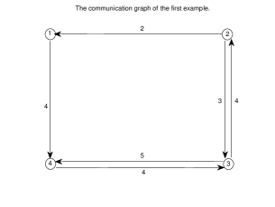
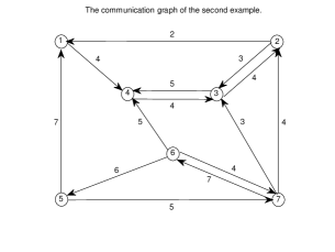
Figure 1: The communication graphs.

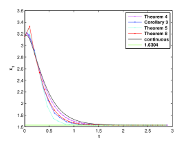
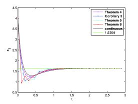
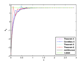
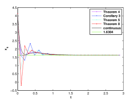
Figure 2: Four agents evolve under the event-triggered principles provided in Theorem 5, Corollary 3, Theorem 6 and Theorem 9 comparing with continuous control.

Then, the parameter $\gamma$ is set to be different values while adopting the triggered principles provided in Theorem 5, Corollary 3 and Theorem 6. The simulation results are list in Table 1, Table 2 and Table 3, respectively. The $T_{1}$ in the table denotes the first time when $\|x(t)-\bar{X}(0)\|\leq 0.0001$, which can be seen as an index representing the convergence speed of the consensus protocol. All the data in this table is the average of 50 runs. It can be seen that all the actual minimum inter-event times are greater than the corresponding $\tau_{0}$ calculated by (22). The minimum value of event interval and the actual number of event decreases with respect to $\gamma$, which is consistent with the theoretical analysis. It is worth noting that $T_{1}$ also decreases with respect to $\gamma$, which is opposite to usually thinking that $T_{1}$ increases with respect to $\gamma$. To sum up, the more close to 1 for $\gamma$, the better for the system to realize a consensus.

$\gamma$	$\tau_{0}$ calculated by (22)	the minimum value of event interval	number of event	$T_{1}$
0.1	0.0044	0.0119	112.88	2.1021
0.2	0.0060	0.0162	81.12	2.0713
0.3	0.0071	0.0193	67.16	2.0524
0.4	0.0080	0.0218	58.78	2.0350
0.5	0.0088	0.0239	53.16	2.0239
0.6	0.0095	0.0257	48.82	2.0062
0.7	0.0100	0.0274	45.54	1.9944
0.8	0.0106	0.0289	42.84	1.9813
0.9	0.0111	0.0302	40.72	1.9748

Table 1: Simulation results with different $\gamma$ under the triggered principles provided in Theorem 5.

$\gamma$	$\tau_{0}$ calculated by (22)	the minimum value of event interval	number of event	$T_{1}$
0.1	0.0044	0.0124	107.40	2.5863
0.2	0.0060	0.0234	56.36	2.4379
0.3	0.0071	0.0333	39.24	2.3251
0.4	0.0080	0.0390	31.00	2.2519
0.5	0.0088	0.0472	25.56	2.1577
0.6	0.0095	0.0478	21.60	2.0541
0.7	0.0100	0.0465	18.46	1.9656
0.8	0.0106	0.0482	17.06	1.9263
0.9	0.0111	0.0483	16.36	1.9058

Table 2: Simulation results with different $\gamma$ under the triggered principles provided in Corollary 3.

$\gamma$	$\tau_{0}$ calculated by (22)	the minimum value of event interval	number of event	$T_{1}$
0.1	0.0044	0.0124	110.70	2.6132
0.2	0.0060	0.0248	53.02	2.4840
0.3	0.0071	0.0371	33.66	2.3436
0.4	0.0080	0.0495	23.92	2.1949
0.5	0.0088	0.0615	18.52	2.0551
0.6	0.0095	0.0719	16.64	1.9798
0.7	0.0100	0.0808	16.32	1.9473
0.8	0.0106	0.0821	14.82	1.8461
0.9	0.0111	0.0787	13.74	1.7856

Table 3: Simulation results with different $\gamma$ under the triggered principles provided in Theorem 6.

Finally, we compare the triggered principles provided in Theorem 5, Corollary 3, Theorem 6, Theorem 9 with $\gamma=0.9$, and $a=0.0666$ and continuous control. The simulation results are list in Table 4. All the data in this table is the average of 50 runs. It can be seen that the triggered principle provided in Theorem 6 is the best, since the corresponding minimum value of event interval is the biggest, the number of event is the smallest and the convergence speed of the consensus protocol is the fastest.

triggered principles	the minimum value of event interval	number of event	$T_{1}$
Theorem 5	0.0281	50.92	2.4554
Corollary3	0.0466	16.36	1.8846
Theorem 6	0.0774	13.18	1.7029
Theorem 9	/	21.58	2.1580
continuous control	/	/	2.7162

Table 4: Simulation results Example 1 with different triggered principles of.

Secondly, we consider a network of seven agents whose Laplacian matrix is given by

$$L=\left[\begin{array}[]{rrrrrrr}-9&2&0&0&7&0&0\\ 0&-8&4&0&0&0&4\\ 0&3&-10&4&0&0&3\\ 4&0&5&-14&0&5&0\\ 0&0&0&0&-6&6&0\\ 0&0&0&0&0&-7&7\\ 0&0&0&0&5&4&-9\end{array}\right].$$

Obviously, this is a asymmetric reducible weighted network with a spanning tree described by Figure 1 right. The seven agents can be divided into two strongly connected components, i.e. the first four agents form a strongly connected component and the rest form anther. The initial value of each agent is also randomly selected within the interval $[-5,5]$ in our simulations. Figure 3 shows the 1st, 3rd, 5th and 7th agents evolve under the triggered principles provided in Theorem 7, Corollary 6, Theorem 8 and Theorem 9 with $\gamma=0.9$, $a^{1}=\frac{\rho_{2}(-Q^{1})}{\rho(\hat{Q}^{1})}=0.0580$, $a^{2}=\frac{\rho_{2}(-Q^{2})}{\rho(\hat{Q}^{2})}=0.0882$ and initial value $[1.3240,-4.0250,-2.2150,0.4690,4.5750,4.6490,-3.4240]^{\top}$, comparing with continuous control, i.e., evolving under (56). Under above initial conditions, the consensus value can be computed, $\nu=2.0409$, and $T_{0}=0.0643$ in Theorem 9. The symbol $\cdot$ indicates the agent’s triggering times.

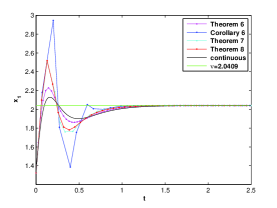
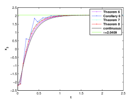
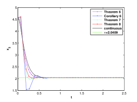
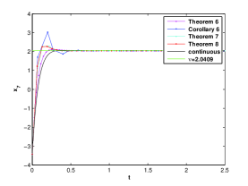
Figure 3: The 1st, 3rd, 5th and 7th agents evolve under the event-triggered principles provided in Theorem 7, Corollary 6, Theorem 8 and Theorem 9 comparing with continuous control.

Finally, we compare the triggered principles provided in Theorem 7, Corollary 6, Theorem 8, Theorem 9 with $\gamma=0.9$, $a^{1}=0.0580$, $a^{2}=0.0882$, and continuous control. The simulation results are list in Table 5. All the data in this table is the average of 50 runs. It can be seen that the triggered principle provided in Theorem 8 is the best, since the corresponding minimum value of event interval is the biggest, the number of event is the smallest and the convergence speed of the consensus protocol is the fastest.

triggered principles	the minimum value of event interval	number of event	$T_{1}$
Theorem 7	0.0232	70.90	2.3220
Corollary 6	0.0402	36.42	2.1177
Theorem 8	0.0559	29.54	2.1063
Theorem 9	/	33.52	2.1549
continuous control	/	/	2.4688

Table 5: Simulation results of Example 2 with different triggered principles.

6 Conclusion

In this paper, we first consider centralized event-triggered strategies for multi-agent systems. The triggering times depend on the ratio of a certain measurement error with respect to the norm of a function of the all agents’ states. It is proved that if the asymmetric network topology has a spanning tree, then the centralized event-triggered coupling strategy we provide can realize consensus exponentially for the multi-agent system and singular triggering and Zeno behavior can be both excluded. Then the results are extended to discontinuous monitoring, where each agent computes its next triggering time in advance without having to observe the system s state continuously and we have pointed out that it is very easy to compute the next triggering time in our principles. In addition, we provide a novel and very simple self-triggered rule (see Theorem 6 for irreducible case, see Theorem 8 for reducible case), and we prove that the time interval length of our rule applied in symmetric topology is bigger comparing with the centralized rule in [11]. Finally, we give a periodic self-triggered strategy. The effectiveness the theoretical results are verified and compared by two examples of numerical simulation. In our numerical simulation, it is worth noting that the time needed to reach consensus decreases with respect to $\gamma$ which is opposite to usually thinking.

In our future paper, inspired by [6, 14], we will focus on the distributed event-triggered and self-triggered strategies with push-based feedback and pull-based feedback for multi-agent systems with asymmetric and reducible topologies.

References

• [1] R. O. Saber, and R. M. Murray, Consensus Problems in Networks of Agents With Switching Topology and Time-Delays, IEEE Trans. Autom. Control, vol. 49, no. 9, pp. 1520–1533, Sep. 2004.
• [2] L. Moreau, Stability of continuous-time distributed consensus algorithms, 43rd IEEE Conference on Decision and Control, 2004. CDC. , vol. 4, pp. 3998-4003, 2004
• [3] R. Wei, and R. W. Beard, Consensus seeking in multiagent systems under dynamically changing interaction topologies, IEEE Trans. Autom. Control, vol. 55, no. 5, pp. 655-661, May 2005.
• [4] L. Cao, Y. F. Zheng, and Q. Zhou, A necessary and sufficient condition for consensus of continuous-time agents over undirected time-varying networks, IEEE Trans. Autom. Control, vol. 56, no. 8, pp. 1915-1920, Aug. 2011.
• [5] B. Liu, W. L. Lu, and T. P. Chen, Consensus in networks of multiagents with switching topologies modeled as adapted stochastic processes, SIAM J. Control optim., vol. 49, no. 1, pp. 227-253, 2011.
• [6] P. Tabuada, Event-triggered real-time scheduling of stabilizing control tasks, IEEE Trans. Autom. Control, vol. 52, no. 9, pp. 1680-1685, Sep. 2007.
• [7] W.P.M.H. Heemels, J.H. Sandee, and P.P.J. Van Den Bosch, Analysis of event-driven controllers for linear systems, Int. J. Control, vol. 81, no. 4, pp. 571-590, 2007.
• [8] X. Wang,and M.D. Lemmon, Event design in event-triggered feedback control systems, in Proc. 47th IEEE Conf. Decision Control, pp. 2105-2110, 2008.
• [9] M. J. Manuel, and P. Tabuada, Decentralized event-triggered control over wireless sensor/actuator networks, IEEE Trans. Autom. Control, vol. 56, no. 10, pp. 2456-2461, Oct. 2011.
• [10] X.Wang, and M. D. Lemmon, Event-triggering distributed networked control systems, IEEE Trans. Autom. Control, vol. 56, no. 3, pp. 586-601, Mar. 2011.
• [11] D. V. Dimarogonas, E. Frazzoli, and K. H. Johansson, Distributed event-triggered control for multi-agent systems, IEEE Trans. Autom. Control, vol. 57, no. 5, pp. 1291-1297, May 2012.
• [12] Z. Liu, Z. Chen, and Z. Yuan, Event-triggered average-consensus of multi-agent systems with weighted and direct topology, Journal of Systems Science and Complexity, vol. 25, no. 5, pp. 845-855, 2012.
• [13] G. S. Seyboth, D. V. Dimarogonas, and K. H. Johansson, Event-based broadcasting for multi-agent average consensus, Automatica, vol. 49, pp. 245-252, 2013.
• [14] Y. Fan, G. Feng, Y. Wang, and C. Song, Distributed event-triggered control of multi-agent systems with combinational measurements, Automatica, vol. 49, pp. 671-675, 2013.
• [15] A. Anta, and P. Tabuada, Self-triggered stabilization of homogeneous control systems, in Proc. Amer. Control Conf., 2008, pp. 4129-4134.
• [16] M. Mazo, and P. Tabuada, On event-triggered and self-triggered control over sensor/actuator networks, in Proc. 47th IEEE Conf. Decision Control, 2008, pp. 435-440.
• [17] X.Wang and M. D. Lemmon, Self-triggered feedback control systems with finite-gain $\mathcal{L}_{2}$ stability, IEEE Trans. Autom. Control, vol. 45, no. 3, pp. 452-467, Mar. 2009.
• [18] M. J. Manuel, A. Anta, and P. Tabuada, An ISS self-triggered implementation of linear controllers, Automatica, vol. 46, no. 8, pp. 1310-1314, 2010.
• [19] A. Anta and P. Tabuada, To sample or not to sample: self-triggered control for nonlinear systems, IEEE Trans. Autom. Control, vol. 55, no. 9, pp. 2030-2042, Sep. 2010.
• [20] R. Diestel, Graph theory, Graduate texts in mathematics 173, New York: Springer-Verlag Heidelberg, 2005.
• [21] R. A. Horn, and C. R. Johnson, Matrix Analysis, Cambridge, U.K.: Cambridge Univ. Press, 1987.
• [22] K.H. Johansson, M. Egerstedt, J. Lygeros, and S.S. Sastry, On the regularization of zeno hybrid automata, Systems and Control Letters, vol. 38, pp. 141-150, 1999.
• [23] T.P. Chen, X.W. Liu, and W.L. Lu, Pinning complex networks by a single controller, IEEE Trans. Circuits and Systems, vol. 54, no. 6, pp. 1317-1326, Jun. 2007.
• [24] C.W. Wu, Synchronization in networks of nonlinear dynamical systems coupled via a directed graph, Nonlinearity, vol. 18, no. 3, pp. 1057-1064, 2005.
• [25] Lu, W., & Chen, T,. (2004). Synchronization Analysis of Linearly Coupled Networks of Discrete Time Systems, Physica D 198 148-168
• [26] Lu, W., & Chen, T,. (2007)., Global Synchronization of Discrete-Time Dynamical Network With a Directed Graph, IEEE Transactions on Circuits and Systems-II: Express Briefs, 54(2), 136-140
• [27] R. Olfati-Saber, J. A. Fax, and R. M. Murray, Consensus and cooperation in networked multi-agent systems, Proc. IEEE, vol. 95, pp. 215-233, 2007.