Interpretation of scanning tunneling quasiparticle interference and impurity states in cuprates

Abstract

We apply a recently developed method combining first principles based Wannier functions with solutions to the Bogoliubov-de Gennes equations to the problem of interpreting STM data in cuprate superconductors. We show that the observed images of Zn on the surface of Bi₂Sr₂CaCu₂O₈ can only be understood by accounting for the tails of the Cu Wannier functions, which include significant weight on apical O sites in neighboring unit cells. This calculation thus puts earlier crude “filter” theories on a microscopic foundation and solves a long standing puzzle. We then study quasiparticle interference phenomena induced by out-of-plane weak potential scatterers, and show how patterns long observed in cuprates can be understood in terms of the interference of Wannier functions above the surface. Our results show excellent agreement with experiment and enable a better understanding of novel phenomena in the cuprates via STM imaging.

Scanning tunneling microscopy (STM) methods were applied to cuprates relatively early on, but dramatic improvements in energy and spatial resolution led to a new set of classic discoveries in the early part of the last decade, giving for the first time a truly local picture of the superconducting and pseudogap states at low temperaturesFischer et al. (2007); Fujita et al. (2012). These measurements revealed gaps that were much more inhomogeneous than had previously been anticipatedCren et al. (2001); Pan et al. (2001); Howald et al. (2001); Lang et al. (2002), exhibited localized impurity resonant statesYazdani et al. (1999); Pan et al. (2000), and gave important clues to the nature of competing orderHowald et al. (2003); Kivelson et al. (2003); Hanaguri et al. (2004); Vershinin et al. (2004); Kohsaka et al. (2007). More recently, STM has again been at the forefront of studies of inhomogeneities, this time as a real space probe of intra-unit cell charge ordering visible in the underdoped systemsFujita et al. (2014). While a microscopic description of such atomic scale phenomena in superconductors is available in terms of the Bogolibuov de-Gennes equations, such calculations are always performed on a lattice with sites centered on the Cu atoms, and thus do not contain intra-unit cell information.

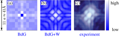
Figure 1: (Color online) (a) Resonant state real-space BdG patterns at $\Omega_{0}=-3.6\,\text{meV}$ as obtained from conventional BdG calculations in logarithmic scale, (b) xy cut through continuous 3D LDOS $(x,y,z\approx 5\text{\AA};\Omega_{0})$ at $\Omega_{0}=-3.6\,\text{meV}$ showing strong similarity to the measured conductance maps (c) reproduced from Ref. [Pan et al., 2000] rotated to match the orientation in (a) and (b) and cropped to 11$\times$11 elementary cells with the impurity located at the center.

The simplest example of a problem that can arise because of the deficiencies of theory in this regard is that of the Zn impurity substituting for Cu in Bi₂Sr₂CaCu₂O₈ (BSCCO), a cuprate material which cleaves well in vacuum, leaving atomically smooth surfaces ideal for STM. The observation of a spectacularly sharp impurity resonance at the impurity siteYazdani et al. (1999); Pan et al. (2000); Machida et al. (2011); Hamidian et al. (2012) was an important local confirmation of unconventional pairing in the cuprates. The differential conductance map near the impurity exhibits a cross-shaped real-space conductance map at resonance, as expected for a pointlike potential scatterer in a $d$-wave superconductor, see Fig. 1(c) Note (1) Upon closer examination, however, the pattern deviates from the expected theoretical one on the Cu square lattice in some important respectsBalatsky et al. (2006); Alloul et al. (2009). First, it displays a central maximum on the impurity site, unlike simple models, which have a minimum (Fig. 1(a)). Second, the longer range intensity tails are rotated 45 degrees from the nodal directions of the $d$-wave gap, where such long quasiparticle decay lengths are expectedBalatsky et al. (2006). There is still no consensus on the origin of this pattern, which has been discussed in terms of nonlocal Kondo correlationsPolkovnikov et al. (2001), postulated extended potentialsFlatté (2000); Tang and Flatté (2002, 2004), Andreev phase impuritiesAndersen et al. (2006), and “filter effects”, which assume that the tunneling process from the surface to the impurity through several insulating layers involves atomic states in several neighboring unit cellsZhu et al. (2000); Martin et al. (2002). So far, these theories have been expressed entirely in terms of phenomenological effective hoppings in the Cu tight-binding model. First principles calculations for Zn in BSCCO in the normal stateWang et al. (2005) provide some evidence in support of the filter picture, but until recently it was not possible to include both superconductivity and the various atomic wave functions extending into the barrier layers responsible for the filter. Nieminen et al. investigated the conductance spectrum in the BSCCO system using an analysis based on atomiclike wave functionsNieminen et al. (2009), and showed that for the homogeneous system it could be decomposed in a series of tunneling paths, as postulated by the earlier crude proposalsZhu et al. (2000); Martin et al. (2002). Using this approach one can explain, e.g., the spectral lineshape at high bias voltage, but presently it is unclear how this approach applies to inhomogeneous problems.

The vast amount of STM data on cuprate surfaces have often been distilled using the quasiparticle interference (QPI), or Fourier transform STM spectroscopy technique, one of the most important modern techniques for unraveling the origin of high temperature superconductivity. This probe is sensitive to the wavelengths of Friedel oscillations caused by disorder, which then, in principle contain information on the electronic structure of the pure systemSprunger et al. (1997); Hoffman et al. (2002). These wavelengths manifest themselves in the form of peaks at wave vectors $\mathbf{q}(\omega)$, which disperse with STM bias $V=\omega/e$ and represent scattering processes of high probability on the given Fermi surface. Many attempts have been made to calculate these patterns assuming simple tight-binding band structures, $d$-wave pairing, and methods ranging from single-impurity $T$ matrixWang and Lee (2003); Capriotti et al. (2003); Pereg-Barnea and Franz (2003); Zhang and Ting (2003); Andersen and Hedegård (2003); Nunner et al. (2006); Nowadnick et al. (2012) to many-impurity solutions of the BdG equationsZhu et al. (2004). While some similarities between the calculated patterns, the simplified so-called “octet model”Wang and Lee (2003), and experiment have been reported, there are always serious discrepancies, typically related not so much to the positions of peaks but rather their shapes and intensities.

In this paper we revisit these classic unsolved problems using a new method called the BdG-Wannier (BdG+W) approachChoubey et al. (2014), which combines traditional solutions of the Bogoliubov-de Gennes (BdG) equations with the microscopic Wannier functions obtained from downfolding density functional theory onto a low-energy effective tight-binding Hamiltonian. We show that the local density of states (LDOS) obtained from the continuum Green’s function for a simple strong nonmagnetic impurity bound state in the BSSCO material with a $d$-wave superconducting gap displays excellent agreement with STM conductance maps (Fig. 1). We show furthermore that the QPI patterns obtained from such states, with generically weaker potentials to simulate out-of-plane native defects, agree much better with experiment than QPI maps obtained in previous theoretical calculations.

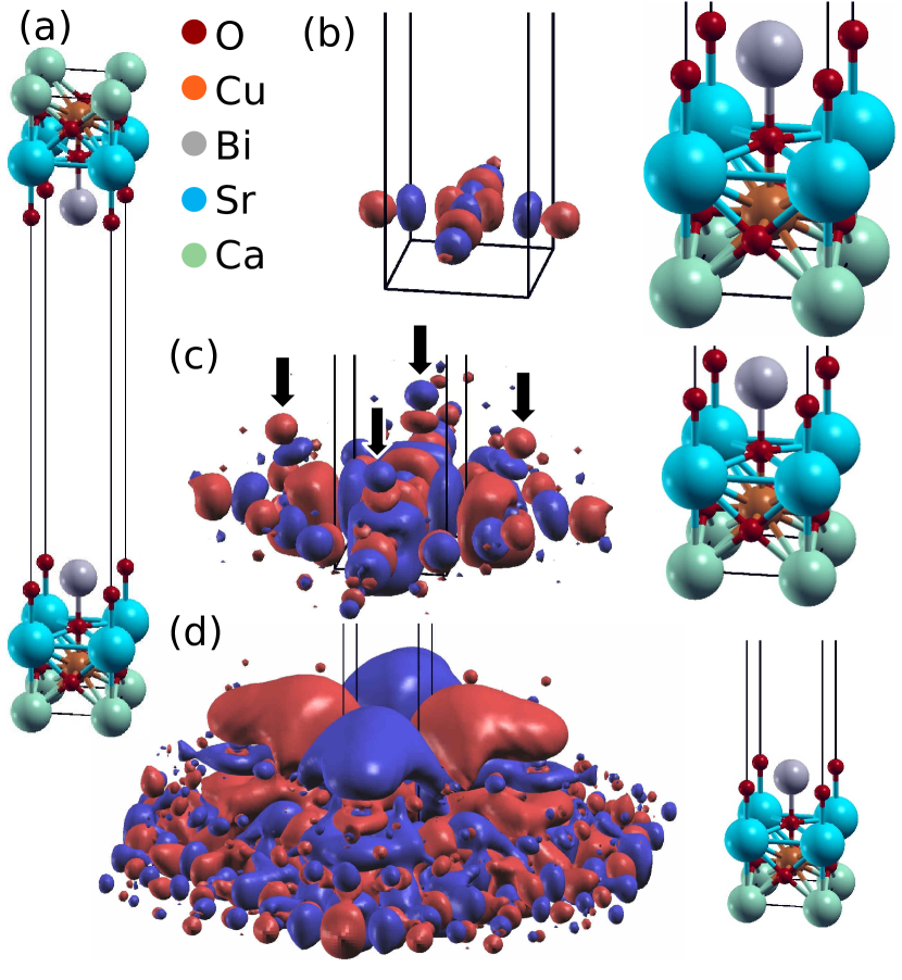
Figure 2: (color online) (a) Elementary cell used in first principles calculation to obtain the electronic structure on the Bi₂Sr₂CaCu₂O₈ surface. Isosurface plots of the Cu-$d_{x^{2}-y^{2}}$ Wannier function at (b) 0.05 bohr^-3/2, (c) 0.005 bohr^-3/2 and (d) 0.0002 bohr^-3/2. Arrows indicate nearest-neighbor apical oxygen tails and red and blue indicate sign of the Wannier function.

Model. The starting point of our investigation is first principles calculations of a BSCCO surface (Fig. 2(a)) that yield a one band tight-binding lattice model for the noninteracting electrons $c_{\mathbf{R}\sigma}$ (with Hamiltonian $H_{0}=\sum_{\mathbf{RR^{\prime}},\sigma}t_{\mathbf{{\mathbf{RR}^{\prime}}}}c_{\mathbf{R}\sigma}^{\dagger}c_{\mathbf{R^{\prime}}\sigma}-\mu_{0}\sum_{\mathbf{R},\sigma}c_{\mathbf{R}\sigma}^{\dagger}c_{\mathbf{R}\sigma}\,,$ where $t_{\mathbf{RR^{\prime}}}$ are hopping elements between unit cells labeled $\mathbf{R}$ and $\mathbf{R}^{\prime}$ and $\mu_{0}$ is the chemical potential), and a Wannier basis $w_{{\mathbf{R}}}({\mathbf{r}})$ with ${\mathbf{r}}$ describing the continuum position. The Wannier function, obtained from a projected Wannier function analysisKu et al. (2002), is primarily of Cu-$d_{x^{2}-y^{2}}$ character with in-plane oxygen $p$-orbital contributions, as can be seen in the isosurface plots for large values of the wave function, Fig. 2(b). However, it also contains contributions from atomic wave functions in neighboring elementary cells, in particular those from the apical oxygen atoms above the Cu plane, Fig. 2(c). These are the main source of the large lobes above the neighboring Cu atoms at the position of the STM tip above the Bi-O plane, Fig. 2(d). There is no weight, however, directly above the center Cu; see Fig. 2(d). This can be understood from the fact that the hybridization of the Cu-$d_{x^{2}-y^{2}}$ orbital with apical O-$p$ and Bi-$p$ orbitals in the same unit cell is forbidden by symmetry. In order to account for correlation effects at low energies, we use a mass renormalization factor of $1/Z=3$ to scale down all hoppings such that the Fermi velocities approximately match the experimentally observed valuesDamascelli et al. (2003) and fix the chemical potential to be at optimal doping, ($n=0.85$).

Next, we solve the inhomogeneous mean field BdG equations for the full Hamiltonian of a superconductor in presence of an impurity $H=H_{0}+H_{\text{BCS}}+H_{\text{imp}},$ where the $d$-wave pairing interaction $\Gamma_{\mathbf{RR^{\prime}}}$ (details in the Supplemental Material Note (2)) enters the calculation of the superconducting order parameter via $\Delta_{\mathbf{RR^{\prime}}}=\Gamma_{\mathbf{RR^{\prime}}}\langle c_{\mathbf{R^{\prime}}\downarrow}c_{\mathbf{R}\uparrow}\rangle$ and gives rise to the second term $H_{\text{BCS}}=-\sum_{\mathbf{R},\mathbf{R^{\prime}}}\Delta_{\mathbf{RR^{\prime}}}c_{\mathbf{R}\uparrow}^{\dagger}c_{\mathbf{R^{\prime}}\downarrow}^{\dagger}+H.c.,$ while the third term is just a nonmagnetic impurity at lattice position $\mathbf{R}^{*}$, e.g. $H_{\text{imp}}=\sum_{\sigma}V_{\text{imp}}c^{\dagger}_{\mathbf{R}^{*}\sigma}c_{\mathbf{R^{*}}\sigma}.$ From the BdG eigenvalues $E_{n\sigma}$ and eigenvectors $u_{n\sigma}$ and $v_{n\sigma}$ we can construct the usual retarded lattice Green’s function

$$\!\,G_{\sigma}({\mathbf{R}},{\mathbf{R}}^{\prime};\omega)\!=\!\sum_{n}\!\left(\!\frac{u^{n\sigma}_{{\mathbf{R}}}u^{n\sigma*}_{{\mathbf{R}}^{\prime}}}{\omega\!-\!E_{n\sigma}\!+\!i0^{+}}\!+\!\frac{v^{n-\sigma}_{{\mathbf{R}}}v^{n-\sigma*}_{{\mathbf{R}}^{\prime}}}{\omega\!+\!E_{n-\sigma}\!+\!i0^{+}}\!\right)\!\!,\!\!\!$$ (1)

and the corresponding continuum Greens functionDell’Anna et al. (2005); Choubey et al. (2014)

$$G_{\sigma}({\mathbf{r}},{\mathbf{r}}^{\prime};\omega)=\sum_{{\mathbf{R}},{\mathbf{R}}^{\prime}}\!G_{\sigma}({\mathbf{R}},{\mathbf{R}}^{\prime};\omega)w_{{\mathbf{R}}}({\mathbf{r}})w^{*}_{{\mathbf{R}}^{\prime}}({\mathbf{r}}^{\prime}),$$ (2)

by a simple basis transformation from the lattice operators $c_{{\mathbf{R}}\sigma}$ to the continuum operators $\psi_{\sigma}({\mathbf{r}})=\sum_{{\mathbf{R}}}c_{{\mathbf{R}}\sigma}w_{{\mathbf{R}}}({\mathbf{r}})$ where the Wannier functions $w_{{\mathbf{R}}}({\mathbf{r}})$ are the matrix elements. A similar transformation has been applied previously to understand neutronWalters et al. (2009) and x-rayLarson et al. (2007); Abbamonte et al. (2008) spectra in the normal state. The continuum Green’s functions can now be used to either calculate the LDOS $\rho({\mathbf{r}},\omega)\equiv-\frac{1}{\pi}\mathop{\text{missing}}{Im}G_{\sigma}({\mathbf{r}},{\mathbf{r}};\omega)$ as measured in STS experimentsTersoff and Hamann (1985) or obtain the QPI patterns by a Fourier transform. Before considering an impurity, we note that the basis transformation in Eq. (2) changes the spectral properties of the Greens function as it also contains terms that are nonlocal in the lattice description, e.g. $G_{\sigma}({\mathbf{R}},{\mathbf{R}}^{\prime};\omega)$ with ${\mathbf{R}}\neq{\mathbf{R}}^{\prime}$. This has implications for the continuum LDOS $\rho({\mathbf{r}},\omega)$, because the sign of $\mathop{\text{missing}}{Im}G_{\sigma}({\mathbf{R}},{\mathbf{R}}^{\prime};\omega)$ is not fixed such that nonlocal contributions will lead to interference effects that can suppress or enhance the continuum LDOS at certain energies. These interference effects between Wannier functions are enhanced at the large distance from the surface where the STM tip is located and the Wannier functions are not confined by the lattice potential. To illustrate this, we show in Fig. 3(c) the spectral dependence of the lattice LDOS for a homogeneous calculation which shows the well-known V-shape. Applying the basis transformation by summing only over terms with ${\mathbf{R}}={\mathbf{R}}^{\prime}$, this behavior is not altered by the continuum LDOS as seen from the overlaied black curve, while in the full expression the spectral dependence is qualitatively modified and displays a clear U-shaped LDOS at low energies. Experimentally obtained conductances reveal exactly such a U-shaped behavior in overdoped samplesKohsaka et al. (2008); McElroy et al. (2005), and the transition from V-shaped LDOS to more U-shaped has been observed with the same tip on samples with spatial inhomogeneous gapsPan et al. (2001); Lang et al. (2002); Alldredge et al. (2008). We believe that these differences can be ascribed to the nonlocal contributions to Eq. (2).

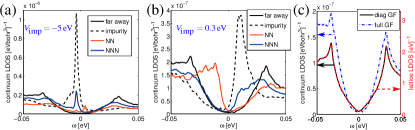
Figure 3: (Color online) (a) Continuum LDOS at $5\text{\AA}$ above the BiO surface in the superconducting state with a single Zn impurity modeled by an onsite $-5\,\text{eV}$ potential. Shown are positions directly above Cu atoms far from the impurity (black), at the impurity position (black, dashed), on the nearest neighbor position (red [light gray]), and on the next-nearest neighbor position (blue [dark gray]), calculated using $20\times 20$ supercells with broadening of $1\;\text{meV}$ and (b) for a weak impurity scatterer with $V_{\text{imp}}=0.3\,\text{eV}$ as used for the QPI analysis. In (c) we compare the spectral properties of the lattice density of states (red [light gray], dashed) with the continuum LDOS above a Cu atom calculated using the diagonal terms of the lattice Greens function $G_{\sigma}({\mathbf{R}},{\mathbf{R}};\omega)$ only (black) and the full Greens function as given in Eq. (2) (blue [gray], dash dotted); all of them calculated for a homogeneous superconductor and scale adjusted such that two curves (black and red [light gray], dashed) exactly overlay.

Zn impurity. A Zn impurity substituting for Cu in BSCCO produces a strong attractive potential which we simply model by an on-site potential of $V_{\text{imp}}=-5\,\text{eV}$, very similar to the value found in our first principles calculation (see Supplemental MaterialNote (2)). Calculating the LDOS, we find a sharp in-gap bound state peak around $\Omega_{0}=-3.6\,\text{meV}$, Fig. 3(a). The lattice LDOS from Eq. (1) shows a minimum at the impurity site and peaks at the NN sites [see Fig. 1(a) and Refs. Balatsky et al. (2006); Alloul et al. (2009)], precisely opposite from the experimental conductance map shown in Fig. 1(c).As pointed out in Refs. Zhu et al. (2000); Wang et al. (2005); Martin et al. (2002); Nieminen et al. (2009), the problem lies in the consideration of the Cu lattice sites far from the BiO surface. The correct quantity to study is the continuum LDOS $\rho({\mathbf{r}},\Omega_{0})$ at the height of the STM tip, which we assume to be at $z=5\,\text{\AA}$ above the BiO surface. The continuum LDOS obtained using Eq. (2) presented in Fig. 1(b) indeed shows a maximum on the impurity site, originating from adding the NN apical oxygen tails of the Cu Wannier functions adjacent to the Zn site, and longer range intensity tails that are rotated 45 degrees from the nodal directions of the $d$-wave gap, in excellent agreement with the experimental observation as taken from Ref.[Pan et al., 2000] Fig. 1(c). We note a discrepancy on the 3rd site along the axis, where some of the reported experimental pattern are more intense than our theoretical resultPan et al. (2000); Machida et al. (2011); Hamidian et al. (2012). However, this peculiar feature seems not to be universal in experimental findings and might either be related to the local disorder environment on the surface of the crystal or the spatial supermodulation. Finer resolution resonances reported in Ref. [Hamidian et al., 2012] are also extremely similar to our calculations. While this is crudely the same agreement reported by “filter”-type theoriesZhu et al. (2000); Martin et al. (2002), our calculation allows many further properties of the pattern to be recognized and provides a simple explanation of why they work. As in Ref. [Wang et al., 2005], the theory allows us to compare the LDOS in the CuO₂ plane to that detected at the surface, but now also includes the redistribution of spectral weight (into, e.g., coherence peaks and impurity bound states) caused by the opening of the superconducting gap.

QPI.

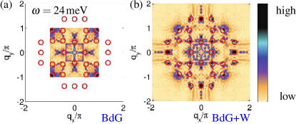
Figure 4: (Color online) Simulated QPI pattern from conductance maps: (a) Fourier transform of the lattice LDOS (BdG) and (b) Fourier transform of the continuum LDOS (BdG+W) at the same energy $\omega=24\,\text{meV}$. Impurity potential for the weak scatterer $V_{\text{imp}}=0.3\,\text{eV}$. The red open symbols indicate the expected positions of the spots from the octet model.

QPI patterns in BSCCO are generated by several different types of disorder, believed to consist primarily of out-of-plane defects such as interstitial oxygens or site switching of Bi and Sr atoms, whose potentials are not known microscopically. To account for these defects, we employ a weak potential scatterer on the Cu site with $V_{\text{imp}}=0.3\,\text{eV}$ and calculate the lattice LDOS and the continuum LDOS $\rho({\mathbf{r}},\omega)$, both of which show only redistribution of spectral weight close to the impurity, compare Fig. 3(b).

Calculating the Fourier transform of the conductances $g({\mathbf{r}},\omega)\propto\rho({\mathbf{r}},\omega)$Hoffman (2011) in order to obtain the conductance maps $|g({\mathbf{q}},\omega)|$ one is immediately faced with the problem that the lattice LDOS only contains information on length scales $\geq a$. Thus, the maps only extend in $\mathbf{q}$ space to the first Brillouin zone $[-\pi/a\ldots\pi/a]$, while the Fourier transform of the continuum LDOS is not restricted in this way. The Fourier transformed maps have often been analyzed in terms of the “octet” model, which predicts a set of seven scattering vectors connecting hot spots at a given energyWang and Lee (2003). To compare to our result, we use the quasiparticle energies of our homogeneous superconductor to derive the expected QPI pattern. Figure 4 shows the calculated conductance maps $|g({\mathbf{q}},\omega)|$ at $\omega=24\,\text{meV}$ for (a) the lattice model (BdG) and (b) the Wannier method (BdG+W) where the $\mathbf{q}$ vectors from the octet model have been marked by circles. In the BdG-only result, a few of the spots are reproduced, others are absent and more importantly, the large $\mathbf{q}$ vectors are not accessible with the lattice model. In contrast, the map generated from the Wannier method shows a much better agreement with the octet model where all spots can be identified and no artificial spots appear. A full scan of energies to visually highlight the dispersive features of the spots can be seen as an animation in the Supplemental MaterialNote (2). Note that it is mathematically not possible to obtain the BdG+W maps from the corresponding BdG maps since the former also contain nonlocal contributions, as explained in Ref. [Choubey et al., 2014].

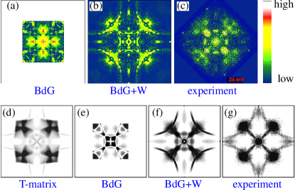
Figure 5: (Color online) (a) QPI Z map obtained from the Fourier transform of the real conventional space BdG patterns at $\omega=24\,\text{meV}$, (b) QPI Z map obtained from the Fourier transform of the continuous 3D LDOS$(x,y,z\approx 5\text{\AA};\omega)$ at $\omega=24\,\text{meV}$ showing strong similarity to (c) the experimental results reproduced from Ref. [Fujita et al., 2014] and rotated to match the orientation in (a) and (b). For the theoretical calculations a weak impurity scatterer of $V_{\text{imp}}=0.3\;\text{eV}$ was used. (d) $T$-matrix scattering interference simulation for $\Lambda(q)$ from Ref. [Fujita et al., 2014], (e) the same obtained from conventional BdG calculations, (f) $\Lambda$ map obtained from the Fourier transform of the continuous 3D LDOS showing strong similarity to the experimental results (g) reproduced from Ref. [Fujita et al., 2014]. All $\bf q$ maps are from $[-2\pi/a\ldots 2\pi/a]$.

In order to compare more closely to experiment, we follow Ref. [Fujita et al., 2014] and simulate the maps of the differential conductance ratios $Z({\mathbf{q}},\omega)$ as well as the energy integrated maps $\Lambda({\mathbf{q}})$ for both approaches, see definition in the Supplemental MaterialNote (2). Figures 5(a-c) show the Z maps of both methods side by side with an experimental result Note (1), demonstrating the improvement of our method (BdG+W) compared to the lattice BdG. Similarly, we compare maps of the integrated ratio $\Lambda({\mathbf{q}})$: In Fig. 5(g) the experimental result is shown next to results from 3 different theoretical methods, (d) $T$-matrix simulation from Ref. [Fujita et al., 2014], (e) lattice BdG and (f) our BdG-Wannier method. While all three theoretical models obtain large weight around $(\pm\pi,\pm\pi)$, in agreement with experiment, only our Wannier method is capable of capturing simultaneously (1) the lines that extend from these large spots to the center, (2) the features along the axes between $\pi$ and $2\pi$ and (3) the arclike features that trace back the Fermi surface as in the analysis of Ref. Fujita et al. (2014).

Conclusions. In this paper we have illustrated the utility of calculating the continuum rather than the lattice Green’s function to compare with STM data in inhomogeneous systems, using a first principles based Wannier function method. We have focused on the cuprate superconductor BSCCO, and calculated the Zn resonant LDOS as well as QPI patterns, showing in both cases dramatic improvement compared to experiment relative to traditional lattice-based BdG analysis. In the case of the Zn impurity, we have provided a first principles high-resolution theory of how electrons are transferred from nearest neighbor unit cells via apical oxygen atoms. In the case of the QPI patterns, the improved agreement is both with experiment and with the “octet” model. This shows that disagreements with the octet model in the past, primarily spurious arclike features and missing peaks, are due to the Fourier transform of the wrong electronic structure information: the lattice density of states in the CuO₂ plane rather than the continuous density of states at the STM tip position. It is clear that our results have implications that go beyond the simple dispersing QPI patterns of a disordered BCS d-wave superconductor. Any new theory of novel phenomena in the CuO₂ plane that seeks to compare with real space or QPI data should now be “dressed” with Wannier information, or risk misidentification of crucial scattering features.

Acknowledgements. The authors are grateful to J. Hoffman, Y. Wang, K. Fujita, and J. C. Davis for useful discussions. P.C., A.K., and P.J.H. were supported by DOE Grant No. DE-FG02-05ER46236, and T.B. as a Wigner Fellow at the Oak Ridge National Laboratory. B.M.A. and A.K. acknowledge support from Lundbeckfond fellowship (grant A9318). W.K. was supported by DOE-BES Grant No. DE-AC02-98CH10886. Work by T.B. was performed at the Center for Nanophase Materials Sciences, a DOE Office of Science user facility.

[Supplemental Material]
In this supplementary material, we collect some technical details of our study, exhibit some additional results illustrating the parameter choices highlighted in the main text, and compare theory and experiment over a wider range of parameters.

First principles based Wannier function calculations. The structural parameters of Bi₂Sr₂CaCu₂O₈ were adopted from Ref. Hybertsen and Mattheiss (1988). We applied the WIEN2KSchwarz et al. (2002) implementation of the full potential linearized augmented plane wave method in the local density approximation. The band structure obtained in our work agrees well with that reported in Ref. Hybertsen and Mattheiss (1988). The calculation was performed for a body-centered tetragonal unit cell terminated at the BiO surface, with a slab of approximately $18.5\,\text{\AA}$ vacuum.

Given the Bloch states $|{\bf k}j\rangle$ corresponding to a set of bands $\epsilon_{{\bf k}j}$, where ${\bf k}$ denotes the crystal momentum and $j$ denotes the band index, one can construct a set of Wannier states $|rn\rangle$ according to $|rn\rangle=\frac{1}{\sqrt{l}}\sum_{{\bf k}j}e^{-i{\bf k}\cdot{\bf R}}|{\bf k}j\rangle U_{jn}({\bf k})$, where $l$ denotes the number of unit cells in the system, ${\bf R}$ denotes the lattice vector and $n$ denotes the Wannier orbital index. The matrix $U_{jn}({\bf k})$ fixes the so called gauge freedom of the Wannier functions. For this purpose we use the projected Wannier function method Ku et al. (2002); Anisimov et al. (2005) in which it is taken to be the projection of $n_{\rm{orb}}$ orbitals $|\varphi_{n}\rangle$ onto the Hilbert space of $n_{\rm{band}}(\geq n_{\rm{orb}})$ bands $|{\bf k}j\rangle$. Given that number of bands in the DFT calculation in this case exceeds the number of Wannier functions, the Wannier transformation is not gauge invariant. In a case like this the projected Wannier function method is preferred because it selects only the correct Hilbert space of the Cu-$d_{x^{2}y^{2}}$ symmetry. When using for example the maximally localization procedureMarzari and Vanderbilt (1997), one risks localizing the Wannier functions at the expense of including other unwanted contributions in the Hilbert space. The Wannier states are constructed by projecting the Cu-$d_{x^{2}-y^{2}}$ orbitals corresponding to the two Cu atoms in the unit cell shown in Fig. 2(a) of the manuscript on a [-3,3]eV window. To simplify the BdG calculation we reduce the resulting two band Hamiltonian to a one band Hamiltonian by cutting the out-of-plane hoppings, since they are an order of magnitude smaller than the in-plane hoppings. The Cu-$d_{x^{2}-y2}$ Wannier function shown in Fig. 2 of the main text consists of a 141$\times$141$\times$67 real space grid centered at Cu and extends over 7$\times$7 unit cells. In Fig. I, the same Wannier function is plotted at 5Å  above the BiO surface on a 501$\times$501 real space grid centered at Cu and extending over 7$\times$7 unit cells such that one can easily see the two features that give rise to the LDOS on the surface which deviates qualitatively from the one in the Cu-O plane: (1) there is no weight above the central Cu atom; (2) dominant weight is at the position of the nearest neighbor Cu atoms and further neighbors.

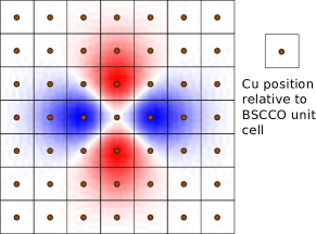
Figure I: (Color online) Plot of the Cu-$d_{x^{2}-y^{2}}$ Wannier function at $5\,\text{\AA}$ above the BiO surface over a region of 7$\times$7 Bi₂Sr₂CaCu₂O₈ (BSCCO) elementary cells.

To calculate the potential of a Zn impurity in Bi₈Sr₈Ca₄Cu₇ZnO₃₂ supercell was used. The k-point mesh was taken to be 7$\times$7$\times$1 for the undoped normal cell and 4$\times$4$\times$1 for the supercell respectively. The basis set sizes were determined by $RK_{\text{max}}=8$. The on-site potential was found to be $-5.6\,\text{eV}$, similar to the value of $-5\,\text{eV}$ used in the calculations described.

Tight binding model.

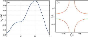
Figure II: (Color online) Band structure (a) and Fermi surface (b) of our one-band tight-binding model for Bi₂Sr₂CaCu₂O₈ at optimal doping.

Table 1: In-plane hoppings with descending magnitude that define our one-band model in Eq. (S1) for Bi₂Sr₂CaCu₂O₈ together with the connection vectors $\mathbf{R-R^{\prime}}$.

	$\mathbf{R-R^{\prime}}$	$t_{\mathbf{R,R^{\prime}}}$ (meV)
$t$	$(\pm 1,0,0)$, $(0,\pm 1,0)$	-465.2
$t^{\prime}$	$(\pm 1,\pm 1,0)$, $(\pm 1,\mp 1,0)$	80.9
	$(\pm 2,0,0)$, $(0,\pm 2,0)$	-65.7
	$(\pm 2,1,0)$, $(1,\pm 2,0)$,$(\pm 2,-1,0)$, $(-1,\pm 2,0)$	-10.5
	$(\pm 3,0,0)$, $(0,\pm 3,0)$	-7.2
	$(\pm 5,0,0)$, $(0,\pm 5,0)$	4.5
	$(\pm 4,0,0)$, $(0,\pm 4,0)$	3.0
	$(\pm 3,1,0)$, $(1,\pm 3,0)$,$(\pm 3,-1,0)$, $(-1,\pm 3,0)$	-2.6
	$(\pm 4,1,0)$, $(1,\pm 4,0)$,$(\pm 4,-1,0)$, $(-1,\pm 4,0)$	1.0

Our tight-binding model

$$H_{0}=\sum_{\mathbf{RR^{\prime}},\sigma}t_{\mathbf{{\mathbf{RR}^{\prime}}}}c_{\mathbf{R}\sigma}^{\dagger}c_{\mathbf{R^{\prime}}\sigma}-\mu_{0}\sum_{\mathbf{R},\sigma}c_{\mathbf{R}\sigma}^{\dagger}c_{\mathbf{R}\sigma}\,,$$ (S1)

describing the noninteracting electrons consists in a one band model with the hopping elements as shown in Table 1. As mentioned in the main text, we fix the chemical potential ($\mu_{0}=-0.0160\,\text{eV}$ without superconductivity) such that the Fermi surface in the normal state approximately matches the optimally doped case with a filling of $n=0.85$ electrons per spin and elementary cell. The corresponding Fermi surface together with the band at a high symmetry cut, which has been renormalized by a factor of $Z=3$ to account for correlations at low energies, are shown in Fig. II.

Superconducting gap. In order to model a d-wave gap in our calculations, we simply take a repulsive nearest neighbor pairing interaction with Hamiltonian

$$H_{\text{BCS}}=-\sum_{\mathbf{RR^{\prime}}}\Gamma_{\mathbf{RR^{\prime}}}c_{\mathbf{R}\uparrow}^{\dagger}c_{\mathbf{R^{\prime}}\downarrow}^{\dagger}c_{\mathbf{R^{\prime}}\downarrow}c_{\mathbf{R}\uparrow}$$ (S2)

where $\Gamma_{\mathbf{RR^{\prime}}}=\Gamma_{0}$ for $\mathbf{R}$ and $\mathbf{R^{\prime}}$ pointing to nearest neighbor elementary cells with $\Gamma_{0}=150\,\text{meV}$ such that the usual mean-field decoupling yields the Hamiltonian cited in the main text. A self-consistent solution of the Bogoliubov-de Gennes (BdG) equations fixing the filling at $n=0.85$ for the homogeneous case in real space yields a converged gap and chemical potential which do not depend on the system size for calculations using more than $N=30$ elementary cells. We therefore use for all further calculations a lattice of 35$\times$35 elementary cells which converges to a $d$-wave gap of $\Delta_{\mathbf{k}}=\Delta_{0}/2[\cos(k_{x})-\cos(k_{y})]$ with the constant $\Delta_{0}\approx 33\,\text{meV}$.

Lattice LDOS pattern for weak scatterer. As mentioned in the main text, the weak scatterer yields only small signatures of the impurity in the real space pattern which then turn into the pattern of the QPI maps when performing a Fourier transform. For completeness, we show in Fig. III and LABEL:fig_weak_scatt2 the analog of Fig. 1 (a) and (b) of the main text for $V_{\text{imp}}=0.3\,\text{eV}$. Experimentally, weak scatterers are present in a large number and of different types such that a comparison with their experimental signatures in real space is not possible. For comparison to experimental data on BSCCO, this value of the potential was chosen simply because the QPI patterns resemble those seen in experiment best. It is interesting to note however that this value does produce an in-gap bound state at around $10\,\text{meV}$, as seen in Fig. 3 of the main text, which corresponds roughly to the positions of the bound states seen for Ni impurities substituted for CuHudson et al. (2001), and the real space patterns seen in Fig. LABEL:fig_weak_scatt2 at nearby energies are extremely similar to that reported in experiment. This comparison will be explored further in a future work.

Figure III: (Color online) Real space BdG patterns at $\omega=-30\ldots 30\,\text{meV}$ as obtained from conventional BdG calculations with the weak scatterer for $V_{\text{imp}}=0.3\,\text{eV}$.

Conductance maps in real space.

The tunneling current in a STM experiment at a given bias voltage $V$ is given byHoffman (2011)

$$I(V,x,y,z)=-\frac{4\pi e}{\hbar}\rho_{t}(0)|M|^{2}\int_{0}^{eV}\rho(x,y,z,\epsilon)d\epsilon\,,$$ (S3)

where $x,y,z$ are the coordinates of the tip, $\rho(x,y,z,\epsilon)$ is the continuum LDOS as defined in the main text, $\rho_{t}(0)$ is the density of states of the tip at the Fermi energy, and $|M|^{2}$ is the square of the the matrix element for the tunneling barrier. Note that the derivation of the above equation assumes an s-wave state in the STM tipTersoff and Hamann (1985) which might not be true in the real experimental situation such that additional matrix element effects might modify the simple proportionality to the integrated LDOS. Taking the derivative with respect to the voltage yields the differential conductance

$$\frac{dI}{dV}=-\frac{4\pi e}{\hbar}\rho_{t}(0)|M|^{2}\rho(x,y,z,eV)\,,$$ (S4)

which is directly proportional to the local density of states a the tip position $\rho(x,y,z,eV)$ at energy $\omega=eV$. Note that the matrix element $|M|^{2}$ can in principle be calculated from the full information of the wave function of the sample, but also requires the knowledge of the wave function of the tip. For simplicity, we do not attempt to model the wave function of the tip and only work with the LDOS because by looking at relative differential conductance maps the matrix elements will drop out later.

The actual units in the corresponding figures of conductance maps are not shown in the main text, in the spirit of this proportionality (Eq. (S4)). Fig. LABEL:fig_weak_scatt2 shows the maps for various energies at the same height including the full information about the units. Fig. LABEL:fig_strong_scatt1 shows the maps of the strong impurity scatterer as in Fig. 1 (b) of the main text, but for different heights above the BiO plane. Looking at the result, one sees that the LDOS rapidly enters the exponential limit as assumed in Tersoff and Hamann (1985) for deriving Eq. (S4): The overall pattern is independent of the actual height, up to an overall scale change (b-f); note that Fig LABEL:fig_strong_scatt1 (a) shows a map very close to the surface where Eq. (S4) is not valid any more. In Fig. LABEL:fig_strong_scatt2, one again recognizes the pattern from the lattice LDOS at the Cu-O plane which is, of course, not the quantity measured in experiments.

Fourier transforms of real space maps.

Figure VIII: (Color online) Fourier amplitudes $g(\mathbf{q},\omega)$ of the conductance maps from lattice BdG (a-f) and continuous LDOS maps (g-l). Energies as indicated in the caption, impurity potential for the weak scatterer $V_{\text{imp}}=0.3\;\text{eV}$.

Once the local density of states for the lattice model as well as the continuum maps at a given height are calculated, it is straightforward to perform a fast Fourier transform to obtain QPI maps. In order to obtain smooth maps in momentum space, we use a fine $\mathbf{k}$-mesh via the zero padding method. This is an interpolation scheme where a larger map in real space with data outside just filled with zeros is Fourier transformed. To avoid large oscillations from the central Bragg peak which will show up in the interpolated result, we remove it manually. A set of Fourier transformed maps of the lattice BdG result and the continuum LDOS (BdG+W) is shown in Fig. VIII for a set of energies within the superconducting gap. Note that the position and the weight of the spots disperse with energy, and the BdG only result is restricted to the first Brillouin zone as explained in the main text.

Octet model. In order to compare our results to the octet modelWang and Lee (2003) which has been successfully used to describe the dispersive behavior of the spots measured in the QPI, we use our tight binding model together with the gap of the homogeneous system to calculate the 8 points in the superconducting state corresponding to the end-points of the banana-shaped isoenergy lines that are shown in Fig LABEL:fig_octet (a) for positive energies. The 7 connecting scattering vectors $\mathbf{q}_{i}(E)$ are defined the same figure, where in (b) the position of the spots (with the corresponding energy color-coded) is plotted to exhibit their dispersion in ${\bf q}$-space. The plot is restricted to positive energies, but the dispersive overall behavior is similar for negative energies, while the actual positions are slightly different because the band structure is not fully symmetric with respect to $E\leftrightarrow-E$.

Relative differential conductance maps and energy integrated maps.

Figure IX: (Color online) Fourier amplitudes of the relative conductance maps $Z(\mathbf{q},\omega)$ from lattice BdG (a-c) and continous ldos maps (BdG+W) (d-f). Energies as indicated in the caption, impurity potential for the weak scatterer $V_{\text{imp}}=0.3\;\text{eV}$.

Figure X: (Color online) Integrated relative conductance maps $\Lambda(\mathbf{q})$ as shown in the main text, but additionally with overlay of the Fermi surface from Fig. II (b) scaled by a factor of two.

[controls,autoplay, palindrome, width=0.6]2./video_figs/134

Figure XI: (Color online) Movie showing the energy evolution of the QPI pattern from conductance maps: (a) Fourier transform with zero padding of the lattice LDOS (BdG) and (b) Fourier transform with zero padding of the continuum LDOS (BdG+W), and (c) density of states of the homogeneous system together with a bar at the actual energy from $\omega=-50\,\text{meV}\ldots 50\,\text{meV}$. Impurity potential for the weak scatterer $V_{\text{imp}}=0.3\,\text{eV}$. The red open symbols indicate the expected positions of the spots from the octet model.

As mentioned above, in the calculation of the conductivity, the matrix elements $|M|^{2}$ have not been taken into account due to lack of information about the wave function of the STM tip. Following e.g. Ref. Fujita et al. (2014), this complication can be avoided by taking the ratio of the differential conductances,

$$Z({\mathbf{r}},\omega)=\frac{g({\mathbf{r}},\omega)}{g({\mathbf{r}},-\omega)}=\frac{\rho({\mathbf{r}},\omega)}{\rho({\mathbf{r}},-\omega)}\,,$$ (S5)

where the matrix elements simply drop out. In the Fourier transform of the ratio $Z(\mathbf{q},\omega)$ the overall structure of the spots becomes a bit more complicated, resulting in additional spurious peaks in the BdG case see Fig. IX (a-c) which are not observed in experiment. The BdG+W results for $Z(\mathbf{q},\omega)$ however compares quite reasonably with experimental results for energies corresponding to a large fraction of the superconducting gap $\Delta_{0}$. Note that a direct comparison of the $Z(\mathbf{q},\omega)$ maps with the expected spots from the octet model is not possible since the maps contain information of the positive and negative energies where the scattering vectors are slightly different, $\mathbf{q}_{i}(E)\neq\mathbf{q}_{i}(-E)$. Recently, a method to trace back the Fermi surface by integrating over the Z maps in energy from zero to the superconducting gap has been introducedFujita et al. (2014); He et al. (2014). The quantity $\Lambda({\bf q})$ is defined as

$$\Lambda({\mathbf{q}})=\int_{0}^{\Delta_{0}}\,d\omega\,Z(\mathbf{q},\omega)\,.$$ (S6)

Performing the integral using our Z maps for energies up to $\Delta_{0}$, we calculate the map presented in Fig. X and also in Fig. 5 (f) of the main text. The arc like features follow the Fermi surface blown up by a factor of two (orange line) because the scattering vector $\mathbf{q}_{4}$ follows the Fermi surface when sweeping in energy and the integral in Eq. (S5) accumulates weight along $2\mathbf{k}_{F}$, such that the method used in Refs. Fujita et al. (2014); He et al. (2014) is demonstrated to work in our simulations.

References

- Fischer et al. (2007) O. Fischer, M. Kugler, I. Maggio-Aprile, C. Berthod, and C. Renner, Rev. Mod. Phys. 79, 353 (2007).
- Fujita et al. (2012) K. Fujita, A. R. Schmidt, E.-A. Kim, M. J. Lawler, D. Hai Lee, J. C. Davis, H. Eisaki, and S.-i. Uchida, J. Phys. Soc. Jpn. 81, 011005 (2012).
- Cren et al. (2001) T. Cren, D. Roditchev, W. Sacks, and J. Klein, Europhys. Lett. 54, 84 (2001).
- Pan et al. (2001) S. H. Pan, J. P. O’Neal, R. L. Badzey, C. Chamon, H. Ding, J. R. Engelbrecht, Z. Wang, H. Eisaki, S. Uchida, A. K. Gupta, K.-W. Ng, E. W. Hudson, K. M. Lang, and J. C. Davis, Nature (London) 413, 282 (2001).
- Howald et al. (2001) C. Howald, P. Fournier, and A. Kapitulnik, Phys. Rev. B 64, 100504 (2001).
- Lang et al. (2002) K. M. Lang, V. Madhavan, J. E. Hoffman, E. W. Hudson, H. Eisaki, S. Uchida, and J. C. Davis, Nature (London) 415, 412 (2002).
- Yazdani et al. (1999) A. Yazdani, C. M. Howald, C. P. Lutz, A. Kapitulnik, and D. M. Eigler, Phys. Rev. Lett. 83, 176 (1999).
- Pan et al. (2000) S. H. Pan, E. W. Hudson, K. M. Lang, H. Eisaki, S. Uchida, and J. C. Davis, Nature (London) 403, 746 (2000).
- Howald et al. (2003) C. Howald, H. Eisaki, N. Kaneko, M. Greven, and A. Kapitulnik, Phys. Rev. B 67, 014533 (2003).
- Kivelson et al. (2003) S. A. Kivelson, I. P. Bindloss, E. Fradkin, V. Oganesyan, J. M. Tranquada, A. Kapitulnik, and C. Howald, Rev. Mod. Phys. 75, 1201 (2003).
- Hanaguri et al. (2004) T. Hanaguri, C. Lupien, Y. Kohsaka, D.-H. Lee, M. Azuma, M. Takano, H. Takagi, and J. C. Davis, Nature (London) 430, 1001 (2004).
- Vershinin et al. (2004) M. Vershinin, S. Misra, S. Ono, Y. Abe, Y. Ando, and A. Yazdani, Science 303, 1995 (2004).
- Kohsaka et al. (2007) Y. Kohsaka, C. Taylor, K. Fujita, A. Schmidt, C. Lupien, T. Hanaguri, M. Azuma, M. Takano, H. Eisaki, H. Takagi, S. Uchida, and J. C. Davis, Science 315, 1380 (2007).
- Fujita et al. (2014) K. Fujita, C. K. Kim, I. Lee, J. Lee, M. H. Hamidian, I. A. Firmo, S. Mukhopadhyay, H. Eisaki, S. Uchida, M. J. Lawler, E.-A. Kim, and J. C. Davis, Science 344, 612 (2014).
- Machida et al. (2011) T. Machida, T. Kato, H. Nakamura, M. Fujimoto, T. Mochiku, S. Ooi, A. D. Thakur, H. Sakata, and K. Hirata, Phys. Rev. B 84, 064501 (2011).
- Hamidian et al. (2012) M. H. Hamidian, I. A. Firmo, K. Fujita, S. Mukhopadhyay, J. W. Orenstein, H. Eisaki, S. Uchida, M. J. Lawler, E.-A. Kim, and J. C. Davis, New J. Phys. 14, 053017 (2012).
- Note (1) The experimental pattern shows a C2 symmetry that is attributed to the structural supermodulation that is not considered in our work.
- Balatsky et al. (2006) A. V. Balatsky, I. Vekhter, and J.-X. Zhu, Rev. Mod. Phys. 78, 373 (2006).
- Alloul et al. (2009) H. Alloul, J. Bobroff, M. Gabay, and P. J. Hirschfeld, Rev. Mod. Phys. 81, 45 (2009).
- Polkovnikov et al. (2001) A. Polkovnikov, S. Sachdev, and M. Vojta, Phys. Rev. Lett. 86, 296 (2001).
- Flatté (2000) M. E. Flatté, Phys. Rev. B 61, R14920 (2000).
- Tang and Flatté (2002) J.-M. Tang and M. E. Flatté, Phys. Rev. B 66, 060504 (2002).
- Tang and Flatté (2004) J.-M. Tang and M. E. Flatté, Phys. Rev. B 70, 140510 (2004).
- Andersen et al. (2006) B. M. Andersen, A. Melikyan, T. S. Nunner, and P. J. Hirschfeld, Phys. Rev. Lett. 96, 097004 (2006).
- Zhu et al. (2000) J.-X. Zhu, C. S. Ting, and C.-R. Hu, Phys. Rev. B 62, 6027 (2000).
- Martin et al. (2002) I. Martin, A. V. Balatsky, and J. Zaanen, Phys. Rev. Lett. 88, 097003 (2002).
- Wang et al. (2005) L.-L. Wang, P. J. Hirschfeld, and H.-P. Cheng, Phys. Rev. B 72, 224516 (2005).
- Nieminen et al. (2009) J. Nieminen, I. Suominen, R. S. Markiewicz, H. Lin, and A. Bansil, Phys. Rev. B 80, 134509 (2009).
- Sprunger et al. (1997) P. T. Sprunger, L. Petersen, E. W. Plummer, E. Lægsgaard, and F. Besenbacher, Science 275, 1764 (1997).
- Hoffman et al. (2002) J. E. Hoffman, K. McElroy, D.-H. Lee, K. M. Lang, H. Eisaki, S. Uchida, and J. C. Davis, Science 297, 1148 (2002).
- Wang and Lee (2003) Q.-H. Wang and D.-H. Lee, Phys. Rev. B 67, 020511 (2003).
- Capriotti et al. (2003) L. Capriotti, D. J. Scalapino, and R. D. Sedgewick, Phys. Rev. B 68, 014508 (2003).
- Pereg-Barnea and Franz (2003) T. Pereg-Barnea and M. Franz, Phys. Rev. B 68, 180506 (2003).
- Zhang and Ting (2003) D. Zhang and C. S. Ting, Phys. Rev. B 67, 100506 (2003).
- Andersen and Hedegård (2003) B. M. Andersen and P. Hedegård, Phys. Rev. B 67, 172505 (2003).
- Nunner et al. (2006) T. S. Nunner, W. Chen, B. M. Andersen, A. Melikyan, and P. J. Hirschfeld, Phys. Rev. B 73, 104511 (2006).
- Nowadnick et al. (2012) E. A. Nowadnick, B. Moritz, and T. P. Devereaux, Phys. Rev. B 86, 134509 (2012).
- Zhu et al. (2004) L. Zhu, W. A. Atkinson, and P. J. Hirschfeld, Phys. Rev. B 69, 060503 (2004).
- Choubey et al. (2014) P. Choubey, T. Berlijn, A. Kreisel, C. Cao, and P. J. Hirschfeld, Phys. Rev. B 90, 134520 (2014).
- Ku et al. (2002) W. Ku, H. Rosner, W. E. Pickett, and R. T. Scalettar, Phys. Rev. Lett. 89, 167204 (2002).
- Damascelli et al. (2003) A. Damascelli, Z. Hussain, and Z.-X. Shen, Rev. Mod. Phys. 75, 473 (2003).
- Note (2) See Supplemental Material, which includes Refs. Hybertsen and Mattheiss (1988); Schwarz et al. (2002); Ku et al. (2002); Anisimov et al. (2005); Hudson et al. (2001); Hoffman (2011); Tersoff and Hamann (1985); Wang and Lee (2003); Fujita et al. (2014); He et al. (2014).
- Dell’Anna et al. (2005) L. Dell’Anna, J. Lorenzana, M. Capone, C. Castellani, and M. Grilli, Phys. Rev. B 71, 064518 (2005).
- Walters et al. (2009) A. C. Walters, T. G. Perring, J.-S. Caux, A. T. Savici, G. D. Gu, C.-C. Lee, W. Ku, and I. A. Zaliznyak, Nat. Phys. 5, 867 (2009).
- Larson et al. (2007) B. C. Larson, W. Ku, J. Z. Tischler, C.-C. Lee, O. D. Restrepo, A. G. Eguiluz, P. Zschack, and K. D. Finkelstein, Phys. Rev. Lett. 99, 026401 (2007).
- Abbamonte et al. (2008) P. Abbamonte, T. Graber, J. P. Reed, S. Smadici, C.-L. Yeh, A. Shukla, J.-P. Rueff, and W. Ku, Proc. Natl. Acad. Sci. U.S.A 105, 12159 (2008).
- Tersoff and Hamann (1985) J. Tersoff and D. R. Hamann, Phys. Rev. B 31, 805 (1985).
- Kohsaka et al. (2008) Y. Kohsaka, C. Taylor, P. Wahl, A. Schmidt, J. Lee, K. Fujita, J. W. Alldredge, K. McElroy, J. Lee, H. Eisaki, S. Uchida, D.-H. Lee, and J. C. Davis, Nature (London) 454, 1072 (2008).
- McElroy et al. (2005) K. McElroy, D.-H. Lee, J. Hoffman, K. Lang, J. Lee, E. Hudson, H. Eisaki, S. Uchida, and J. Davis, Phys. Rev. Lett. 94, 197005 (2005).
- Alldredge et al. (2008) J. W. Alldredge, J. Lee, K. McElroy, M. Wang, K. Fujita, Y. Kohsaka, C. Taylor, H. Eisaki, S. Uchida, P. J. Hirschfeld, and J. C. Davis, Nat. Phys. 4, 319 (2008).
- Hoffman (2011) J. E. Hoffman, Rep. Prog. Phys. 74, 124513 (2011).
- Hybertsen and Mattheiss (1988) M. S. Hybertsen and L. F. Mattheiss, Phys. Rev. Lett. 60, 1661 (1988).
- Schwarz et al. (2002) K. Schwarz, P. Blaha, and G. Madsen, Comput. Phys. Commun. 147, 71 (2002).
- Anisimov et al. (2005) V. I. Anisimov, D. E. Kondakov, A. V. Kozhevnikov, I. A. Nekrasov, Z. V. Pchelkina, J. W. Allen, S.-K. Mo, H.-D. Kim, P. Metcalf, S. Suga, A. Sekiyama, G. Keller, I. Leonov, X. Ren, and D. Vollhardt, Phys. Rev. B 71, 125119 (2005).
- Marzari and Vanderbilt (1997) N. Marzari and D. Vanderbilt, Phys. Rev. B 56, 12847 (1997).
- Hudson et al. (2001) E. W. Hudson, K. M. Lang, V. Madhavan, S. H. Pan, H. Eisaki, S. Uchida, and J. C. Davis, Nature (London) 411, 920 (2001).
- He et al. (2014) Y. He, Y. Yin, M. Zech, A. Soumyanarayanan, M. M. Yee, T. Williams, M. C. Boyer, K. Chatterjee, W. D. Wise, I. Zeljkovic, T. Kondo, T. Takeuchi, H. Ikuta, P. Mistark, R. S. Markiewicz, A. Bansil, S. Sachdev, E. W. Hudson, and J. E. Hoffman, Science 344, 608 (2014).