July 7th, 2014

FROM QUANTUM FIELD THEORY TO NANO-OPTICS :

REFRACTIVE PROPERTIES OF GRAPHENE IN A MEDIUM-STRONG EXTERNAL MAGNETIC FIELD

O. Coquand , B. Machet

Abstract: 1-loop quantum corrections are shown to induce large effects on the refraction index $n$ inside a graphene strip in the presence of an external magnetic field $B$ orthogonal to it. To this purpose, we use the tools of Quantum Field Theory to calculate the photon propagator at 1-loop inside graphene in position space, which leads to an effective vacuum polarization in a brane-like theory of photons interacting with massless electrons at locations confined inside the thin strip (its longitudinal spread is considered to be infinite). The effects factorize into quantum ones, controlled by the value of $B$ and that of the electromagnetic coupling $\alpha$, and a “transmittance function” $U$ in which the geometry of the sample and the resulting confinement of electrons play the major roles. We consider photons inside the visible spectrum and magnetic fields in the range 1-20  Teslas. At $B=0$, quantum effects depend very weakly on $\alpha$ and $n$ is essentially controlled by $U$; we recover, then, an opacity for visible light of the same order of magnitude $\pi\alpha_{vac}$ as measured experimentally.

1 Introduction

Very strong magnetic fields $B$ are known to induce dramatic effects on the spectrum of hydrogen and on the critical number $Z_{c}$ of atoms [1] [2]. However, the typical effects being ${\cal O}(\frac{e^{3}B}{m_{e}})$, gigantic fields are needed, $\geq 10^{16}$ Gauss, which are out of reach on earth.

The property that the fine structure constant $\alpha$ in graphene largely exceeds $1$ [3] instead of its vacuum value $\alpha_{vac}\simeq\frac{1}{137}$ was a sufficient motivation to investigate whether sizable effects could be obtained at lower cost in there.

While graphene in an external magnetic field is usually associated to the so-called “abnormal quantum hall effect” [3] [4], our results show that one can also expect optical effects for the visible spectrum and “reasonable” values of the magnetic field.

This work relies on the Schwinger formalism [5] [6] to write the propagator of the Dirac-like massless electrons inside graphene in an external magnetic field $B$ perpendicular to the graphene strip, and on a calculation in position space of the photon propagator at 1-loop. This enables in particular to explicitly constrain the vertices of electrons with photons to stay confined inside the graphene strip . So doing, we get an effective 1-loop vacuum polarization $\Pi^{\mu\nu}_{eff}$ that can be plugged in the light-cone equations derived according to the pioneering work of Tsai and Erber [7], and of Dittrich and Gies [8].

One of the salient features of the effective $\Pi^{\mu\nu}_{eff}$ is that it factorizes into the 1-loop $\Pi^{\mu\nu}$ calculated with the standard rules of Quantum Field Theory (QFT) in the presence of an external magnetic field, adapted of course to the case of the Hamiltonian for graphene at the Dirac points, times a universal function $U$ which does not depend on the magnetic field, but only on the energy $q_{0}$ of the photon, of the relative penetration $u$ inside the graphene strip (very weakly), and of its “geometry” (in a somewhat extended meaning). It is classical by nature and shares similarities with the so called “transmittance” function in optics or “transfer function” in electronics. The genuine $\Pi^{\mu\nu}$ concentrates all quantum effects and those of the magnetic field.

It is also a remarkable fact that, though electrons inside graphene correspond classically to massless $3+1$ Dirac electrons with a vanishing momentum $p_{3}$ along the direction of $B$, the quantum calculation of the photon propagator at 1-loop shows that the latter can nevertheless exchange momentum with virtual electrons in the direction of $B$ as expected from quantum mechanics and their confinement inside the small width $2a$ of the graphene strip: the corresponding unavoidable “energy-momentum non-conservation” of photons along $B$ is found indeed to be the quantum uncertainty $\hbar/a$ on the electron momentum.

The effects that we describe only concern photons with “parallel” polarization (see [7]) (for transverse polarization, the only solution that we found to the light-cone equation is the trivial $n=1$). The large value of the electromagnetic coupling turns out not to be only amplifying factor. That the massless Dirac electrons of graphene that interact with photons are confined inside a thin strip plays also a major role.

The effects of the confinement of electrons that arise add to the ones that have, for example, been investigated in [9] when the longitudinal size $L$ of graphene is finite. Confinement conspires with the external magnetic field to produce macroscopic effects. The difference is that we are concerned here with the confinement in the “short” direction, the thickness $2a\approx 350\,pm$ of graphene, considering that its large direction $L$ is like infinite . This makes an intuitive physical interpretation much less easy since, now, no cyclotron radius can eventually reach the (longitudinal) size of the graphene strip.

The refractive index $n=n_{1}+i\,n_{2}$ is found to essentially depend on $\alpha$, on the angle of incidence $\theta$, and on the ratio $\Upsilon=\frac{\sqrt{2eB}}{q_{0}}$. In the absence of any external $B$, its dependence on the electromagnetic coupling fades away, and it is mainly constrained by the sole property that electrons are confined.

A transition occurs at small angle of incidence $\theta_{min}\sim\frac{1}{\Upsilon}$: no solution with $|n_{2}|\ll n_{1}$ to the light-cone equation exists anymore for $\theta<\theta_{min}$. There are hints that the system goes brutally to a regime with large index/absorption. The identification of the corresponding solutions however requires more elaborate numerical techniques, which will be the object of a subsequent work.

That the final results differ from what would be obtained from $QED_{2+1}$ is expected since the gauge field, unlike the electrons, lives in $3+1$ dimension and the framework of our calculations is more a “brane-like” picture for graphene.

Our calculations are made in the limit of a “medium-strong” $B$, in the sense that $\sqrt{2eB}\gg q_{0}$, and are only valid at this limit such that, in particular, the case $B=0$ is not directly accessible. This is why we have performed a special calculation for $B=0$ the end of the study. $B$ is however not considered to be “infinite” like in [1] [2] [10]. They also require $aq_{0}\ll 1$, in which $2a$ is the thickness of the graphene strip. This last approximation guarantees to stay in the linear part of the electron spectrum close to the Dirac point, which is an essential ingredient to use a “Dirac-like” effective Hamiltonian [3]. We are concerned with photons in the visible spectrum, which sets us very far from geometrical optics , and limit $B$, for the sake of experimental feasibility, to 20 Teslas.

Our results are summarized in the 2 plots of Figure 4.

The last section is dedicated to the case when no external magnetic field is present. We show in this case that no $\theta_{min}$ exists and that, instead, when the angle of incidence gets smaller and smaller, the refraction index $n$ goes continuously from “quasi-real” values to complex values with larger $n_{1}$ and $n_{2}$. At very small values of $\theta$, we recover an opacity of the same order of magnitude as the one measured experimentally [11].

The literature dedicated to graphene is enormous and we cannot unfortunately pay a tribute to the whole of it. We only make few citations, but the reader can find, in particular inside the reviews articles, references to most of the important works.

2 From the vacuum polarization to light-cone equations and to the refraction index

2.1 Conventions and setting

Let us follow Tsai-Erber [7]. $\vec{B}$ is $\parallel z$, the $\vec{q}$ of the propagating photon (plane wave) is chosen to lie in the $(x,z)$ plane. See Fig. 1.

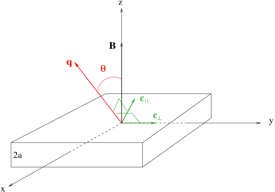
Figure 1: $\vec{B}$ is perpendicular to the graphene strip of width $2a$. The polarization vector $\vec{\epsilon}$, perpendicular to the momentum $\vec{q}$ of the electromagnetic wave, is decomposed into $\vec{\epsilon}_{\parallel}$ in the $(x,z)$ plane and $\vec{\epsilon}_{\perp}$ perpendicular to this plane.

We shall call $\theta$ the “angle of incidence”; the reader should keep in mind that, since we are concerned with the propagation of light inside graphene, $\theta$ is the angle of incidence of light inside this medium.

The polarization vector $\vec{\epsilon}$  is decomposed into $\vec{\epsilon}_{\parallel}$ and $\vec{\epsilon}_{\perp}$, both orthogonal to $\vec{q}$. $\vec{\epsilon}_{\perp}\parallel y$ and $\vec{\epsilon}_{\parallel}$ is in the $(x,z)$ plane. If we call $\theta$ the angle $(\vec{B},\vec{q})$, $\vec{\epsilon}_{\parallel}=-\cos\theta\,\vec{i}+\sin\theta\,\vec{k}$, while $\vec{\epsilon}_{\perp}=\vec{j}$. One has $\vec{q}=|\vec{q}|\,(\sin\theta\,\vec{i}+\cos\theta\,\vec{k})$. We shall call $\vec{\epsilon}_{\parallel}$ “parallel polarization” and $\vec{\epsilon}_{\perp}$ “transverse polarization”. It must be noticed that, at normal incidence $\theta=0$, there is no longer a plane $(\vec{q},B)$ such that these 2 polarizations can no longer be distinguished.

We shall in the following use “hatted” letters for vectors living in the Lorentz subspace $(0,1,2)$. For example

$$\hat{q}=(q^{0},q^{1},q^{2}),\quad q=(\hat{q},q_{3})=(q_{0},q_{1},q_{2},q_{3}).$$ (1)

2.2 The modified Maxwell Lagrangian and the light-cone equations

Taking into account the contribution of vacuum polarization, the Maxwell Lagrangian gets modified to [8]

$${\cal L}(x)=-\frac{1}{4}F_{\mu\nu}(x)F^{\mu\nu}(x)-\frac{1}{2}\int d^{4}y\;A^{\mu}(x)\Pi_{\mu\nu}(x,y,B)A^{\nu}(y),$$ (2)

from which one gets the Euler-Lagrange equation

$$\Big{(}g_{\mu\nu}\,q^{2}-q_{\mu}q_{\nu}+\Pi_{\mu\nu}(q,B)\Big{)}A^{\nu}(q)=0.$$ (3)

Left-multiplying (3) with

$$A^{\mu}=\alpha\epsilon^{\mu}_{\perp}+\beta\epsilon^{\mu}_{\parallel},$$ (4)

yields

$$\begin{split}&(\alpha\epsilon^{\mu}_{\perp}+\beta\epsilon^{\mu}_{\parallel})\Big{(}g_{\mu\nu}\,q^{2}-q_{\mu}q_{\nu}+\Pi_{\mu\nu}(q,B)\Big{)}(\alpha\epsilon^{\nu}_{\perp}+\beta\epsilon^{\nu}_{\parallel})=0,\cr&\epsilon^{\mu}_{\perp}=(0,0,1,0),\quad\epsilon^{\mu}_{\parallel}=(0,-c_{\theta},0,s_{\theta}),\qquad c_{\theta}\equiv\cos\theta,\ s_{\theta}\equiv\sin\theta.\end{split}$$ (5)

We shall identify $\Pi^{\mu\nu}$ with the effective polarization inside graphene $\Pi^{\mu\nu}_{eff}$ that we shall calculate in section 4 and therefore consider in the following, instead of (3), the Euler-Lagrange equation

$$\Big{(}g^{\mu\nu}\,q^{2}-q^{\mu}q^{\nu}+\Pi^{\mu\nu}_{eff}(q,B)\Big{)}A_{\nu}(q)=0.$$ (6)

As we shall see there, $\Pi_{eff}^{03}=0=\Pi_{eff}^{13}=\Pi_{eff}^{23}$, such that we shall be concerned with the simplified light-cone equation

$$(\alpha^{2}+\beta^{2})q^{2}+\left(\alpha^{2}\Pi_{eff}^{22}(q,B)+\beta^{2}\left(c_{\theta}^{2}\;\Pi_{eff}^{11}(q,B)+s_{\theta}^{2}\;\Pi_{eff}^{33}(q,B)\right)+2\alpha\beta\,c_{\theta}\,\Pi_{eff}^{12}(q,B)\right)=0.$$ (7)

$\vec{q}$ has been furthermore chosen to lie in the $(x,z)$ plane, so $q_{2}=0$, which entails (see (32)) $\Pi^{02}_{eff}=0=\Pi_{eff}^{20},\Pi^{12}_{eff}=0=\Pi_{eff}^{21}$, and the light-cone relation finally shrinks to

$$(\alpha^{2}+\beta^{2})q^{2}+\left(\alpha^{2}\Pi_{eff}^{22}(q,B)+\beta^{2}\left(c_{\theta}^{2}\;\Pi_{eff}^{11}(q,B)+s_{\theta}^{2}\;\Pi_{eff}^{33}(q,B)\right)\right)=0.$$ (8)

Depending of the polarization of the photon, there are accordingly 2 different light-cone relations:
$\bullet$ for $A^{\mu}_{\perp}(q_{0},q_{1},0,q_{3})$, $\alpha=1,\beta=0$,

$$q^{2}+\Pi_{eff}^{22}(q,B)=0;$$ (9)

$\bullet$  for $A^{\mu}_{\parallel}(q_{0},q_{1},0,q_{3})$, $\alpha=0,\beta=1$,

$$q^{2}+\Big{(}c_{\theta}^{2}\;\Pi_{eff}^{11}(q,B)+s_{\theta}^{2}\;\Pi_{eff}^{33}(q,B)\Big{)}=0.$$ (10)

One of the main features of (10) is the occurrence of $\Pi^{33}_{eff}$, which would not be there in $QED_{2+1}$. We shall see later that this term plays an important role.

A remark is due concerning eq. (3). It derivation from the effective Lagrangian (2) relies on the property that $\Pi_{\mu\nu}(x,y)$ is in reality a function of $(x-y)$ only. This is however not the case for $\Pi^{\mu\nu}_{eff}$ which, as we shall see, depends indeed on $(\hat{x}-\hat{y})$ but individually on $x_{3}$ and $y_{3}$ (see the first remark at the end of subsection 4.1.2). Once the dependence on $(x_{3}-y_{3})$ has been extracted, there is a left-over dependence on $y_{3}$, which finally yields for our results the dependence of the refraction index on $u=\frac{y_{3}}{a}\in[-1,+1]$. We shall see however that this dependence is always extremely weak, and we consider therefore the Euler-Lagrange equation (6) to be valid to a very good approximation.

2.3 The refractive index

We define it in a standard way by

$$n=\frac{|\vec{q}|}{q_{0}}.$$ (11)

In practice, $\Pi^{\mu\nu}_{eff}$ is not only a function of $q$ and $B$, but of the angle of incidence $\theta$ and of the relative depth $u$ inside the graphene strip, $u\in[-1,+1]$. The light-cone equations therefore translate into relations $n=n(\theta,B,q_{0},u)$ that we will write explicitly after calculating $\Pi^{\mu\nu}$ and $\Pi^{\mu\nu}_{eff}$.

3 Calculation of the 1-loop vacuum polarization $\boldsymbol{\Pi^{\mu\nu}}(\hat{q},B)$ in the presence of an external magnetic field $\boldsymbol{B}$

Figure 2: The vacuum polarization $\Pi^{\mu\nu}$

It is given by

$$i\Pi^{\mu\nu}(\hat{q},B)=+e^{2}\int_{-\infty}^{+\infty}\frac{d^{3}\hat{p}}{(2\pi)^{3}}\;Tr\;\left[\gamma^{\mu}G(\hat{p},B)\gamma^{\nu}G(\hat{p}+\hat{q},B)\right],$$ (12)

in which $G(\hat{p},B)$ is the propagator of a massless Dirac electron obtained from the Hamiltonian of graphene at the Dirac points, making use of the formalism of Schwinger [5][12] to account for the external magnetic field $B$.

3.1 The electron propagator in an external magnetic field

Following Schwinger (([5], eqs.  2.7 to 2.10), we define the electron propagator as

$$G(x,y)=i\langle(\psi(x)\bar{\psi}(y))_{+}\rangle\Theta(x-y).$$ (13)

The graphene at the Dirac points is described (see for example [3] [4]) by a Hamiltonian which is exactly Dirac in 4 dimensions but with $m_{e}=0$ and $p_{3}=0$ (and the $\gamma$ matrices taken in the chiral representation).

The propagator of an electron inside graphene will accordingly be taken to be [5][12]

$$\hskip-28.45274ptG(\hat{p},B)=\int_{0}^{\infty}d\tau\;\exp\left[-\tau\left((-p_{0}^{2})+\frac{\tanh(e\tau B)}{e\tau B}(p_{1}^{2}+p_{2}^{2})\right)\right]\left((\gamma^{0}p^{0})(1-i\gamma^{1}\gamma^{2}\tanh(e\tau B))-\frac{\gamma_{1}p_{1}+\gamma_{2}p_{2}}{\cosh^{2}(e\tau B)}\right),$$ (14)

which only depends on $\hat{p}=(p_{0},p_{1},p_{2})$ and $B$.

3.1.1 Expanding at “large” $\boldsymbol{B<\infty}$

At the limit $B\to\infty$ , (14) becomes

$$G(\hat{p},B)\stackrel{{\scriptstyle B=\infty}}{{\to}}-e^{-\frac{p_{\perp}^{2}}{eB}}\;\frac{\gamma^{0}p^{0}}{p_{0}^{2}}(1-i\gamma^{1}\gamma^{2}),\quad p_{\perp}^{2}=p_{1}^{2}+p_{2}^{2}.$$ (15)

We shall in this work go one step further in the expansion of $G$ at large $B$: we keep the first subleading terms in the expansions of $\tanh(\tau eB)$ and $\cosh(\tau eB)$ of (14) :

$$\tanh(\tau eB)\approx 1-2e^{-2\tau eB},\quad\cosh^{2}(\tau eB)\approx\frac{e^{2\tau eB}+2}{4}\Rightarrow\frac{1}{\cosh^{2}(\tau eB)}\approx\frac{4\,e^{-2\tau eB}}{1+2\,e^{-2\tau eB}}.$$ (16)

This gives (we note $(\gamma p)_{\perp}=\gamma_{1}p_{1}+\gamma_{2}p_{2}$), still for graphene,

$$\begin{split}G(\hat{p},B)\approx&\int_{0}^{\infty}d\tau\;e^{-\tau(-p_{0}^{2})}e^{-\frac{p_{\perp}^{2}}{eB}(1-2e^{-2e\tau B})}(\gamma^{0}p^{0})(1-i\gamma^{1}\gamma^{2}(1-2e^{-2e\tau B}))\cr&-4(\gamma p)_{\perp}\int_{0}^{\infty}d\tau\;e^{-2e\tau B}\frac{1}{1+2e^{-2e\tau B}}e^{-\tau(-p_{0}^{2})}e^{-\frac{p_{\perp}^{2}}{eB}(1+2e^{-2e\tau B})}.\end{split}$$ (17)

We shall further approximate $e^{-\frac{p_{\perp}^{2}}{eB}(1-2e^{-2e\tau B})}\approx e^{-\frac{p_{\perp}^{2}}{eB}}$, which can be seen to be legitimate because the exact integration yields subleading corrections $\propto 1/(eB)^{2}$, while the ones that we keep are $\propto 1/eB$. This gives

$$\begin{split}G(\hat{p},B)\approx&e^{-\frac{p_{\perp}^{2}}{eB}}\left(-\frac{\gamma^{0}p^{0}}{p_{0}^{2}}(1-i\gamma^{1}\gamma^{2})+2\frac{\gamma^{0}p^{0}}{p_{0}^{2}-2eB}(-i\gamma^{1}\gamma^{2})\right)-4(\gamma p)_{\perp}e^{-\frac{p_{\perp}^{2}}{eB}}\int_{0}^{\infty}d\tau\;\frac{1}{1+2e^{-2e\tau B}}e^{-\tau(-p_{0}^{2}+2eB)}.\end{split}$$ (18)

One has

$$\int_{0}^{\infty}d\tau\;\frac{1}{1+2e^{-2e\tau B}}e^{-\tau(-p_{0}^{2}+2eB)}=(-2)^{-1+\frac{p_{0}^{2}}{2eB}}\frac{\beta(-2,1-\frac{p_{0}^{2}}{2eB},0)}{2eB},$$ (19)

such that (18) rewrites

$$\hskip-14.22636ptG(\hat{p},B)=-e^{-\frac{p_{\perp}^{2}}{eB}}\left(\frac{\gamma^{0}}{p^{0}}\left(1+i\gamma_{1}\gamma_{2}\;\frac{p_{0}^{2}+2eB}{p_{0}^{2}-2eB}\right)+4\frac{p_{1}\gamma_{1}+p_{2}\gamma_{2}}{2eB}F(\frac{p_{0}^{2}}{2eB})\right),\quad F(x)=(-2)^{(-1+x)}\beta(-2,1-x,0),$$ (20)

in which $\beta$ is the incomplete beta function.

When $B<\infty$, corrections arise with respect to (15), which exhibit in particular poles at $p_{0}^{2}=2eB$ (first and 2nd term) and also $p_{0}^{2}=2n\,eB,n=1,2\ldots$ (second term) .

3.1.2 Our working approximation

The expression (20) is still not very simple to use. This is why we shall further approximate $F(x)$ and take

$$F(x)\approx\frac{1}{1-x},$$ (21)

which amounts to only select, in there, the pole at $p_{0}^{2}=2eB$ and neglect the other poles. This approximation is reasonable in the vicinity of this pole, for $0\leq x\leq 1.5$, that is $0\leq p_{0}^{2}\leq 1.5\times(2eB)$, low energy (massless) electrons. It will be discussed more in subsection 5.7 in which we show that the approximation is valid for electrons with energy $p_{0}\leq 10\,eV$ at the weakest magnetic fields $B=1\,T$ that we consider..

We shall accordingly take

$$\begin{split}G(\hat{p},B)&\approx-e^{-\frac{p_{1}^{2}+p_{2}^{2}}{eB}}\left[\frac{\gamma^{0}}{p^{0}}\left(1+i\gamma_{1}\gamma_{2}\;\frac{p_{0}^{2}+2eB}{p_{0}^{2}-2eB}\right)-4\frac{p_{1}\gamma_{1}+p_{2}\gamma_{2}}{p_{0}^{2}-2eB}\right].\end{split}$$ (22)

This leads to expressions much easier to handle, and enables to go a long way analytically.

3.2 Calculation and results

There are 2 steps in the calculation. First one has to perform the traces on the Dirac $\gamma$ matrices, then do explicitly the integration over the loop variable $\hat{p}$.

3.2.1 Performing the traces of $\boldsymbol{\gamma}$ matrices

This step already yields

$$\Pi^{i3}=0=\Pi^{3i},\quad i=0,1,2.$$ (23)

3.2.2 Doing the integrations

Details of the calculation will be given somewhere else. We just want here to present its main steps, taking the example of $\Pi^{00}$. After doing the traces, one gets

$$\begin{split}i\Pi^{00}(\hat{q},B)&=4\,e^{2}\int_{-\infty}^{+\infty}\frac{dp_{0}dp_{1}dp_{2}}{(2\pi)^{3}}e^{-p_{\perp}^{2}/eB}e^{-(p+q)_{\perp}^{2}/eB}\cr&\left(\frac{1}{p_{0}}\frac{1}{p_{0}+q_{0}}+\frac{1}{p_{0}}\frac{p_{0}^{2}+2eB}{p_{0}^{2}-2eB}\frac{1}{p_{0}+q_{0}}\frac{(p_{0}+q_{0})^{2}+2eB}{(p_{0}+q_{0})^{2}-2eB}+16\frac{p_{1}(p_{1}+q_{1})+p_{2}(p_{2}+q_{2})}{(p_{0}^{2}-2eB)((p_{0}+q_{0})^{2}-2eB)}\right),\end{split}$$ (24)

which decomposes into

$$\begin{split}i\Pi^{00}(\hat{q},B)&=I(\hat{q},B)+J(\hat{q},B)+K(\hat{q},B),\cr I(\hat{q},B)&=4\,e^{2}\int_{-\infty}^{+\infty}\frac{dp_{0}dp_{1}dp_{2}}{(2\pi)^{3}}e^{-p_{\perp}^{2}/eB}e^{-(p+q)_{\perp}^{2}/eB}\frac{1}{p_{0}}\frac{1}{p_{0}+q_{0}},\cr J(\hat{q},B)&=4\,e^{2}\int_{-\infty}^{+\infty}\frac{dp_{0}dp_{1}dp_{2}}{(2\pi)^{3}}e^{-p_{\perp}^{2}/eB}e^{-(p+q)_{\perp}^{2}/eB}\frac{1}{p_{0}}\frac{p_{0}^{2}+2eB}{p_{0}^{2}-2eB}\frac{1}{p_{0}+q_{0}}\frac{(p_{0}+q_{0})^{2}+2eB}{(p_{0}+q_{0})^{2}-2eB},\cr K(\hat{q},B)&=4\,e^{2}\int_{-\infty}^{+\infty}\frac{dp_{0}dp_{1}dp_{2}}{(2\pi)^{3}}e^{-p_{\perp}^{2}/eB}e^{-(p+q)_{\perp}^{2}/eB}16\frac{p_{1}(p_{1}+q_{1})+p_{2}(p_{2}+q_{2})}{(p_{0}^{2}-2eB)((p_{0}+q_{0})^{2}-2eB)}.\end{split}$$ (25)

It is then convenient to introduce

$$\begin{split}B(q_{0})&=\int_{-\infty}^{+\infty}dp_{0}\frac{1}{p_{0}}\frac{1}{p_{0}+q_{0}},\cr C(q_{0},B)&=\int_{-\infty}^{+\infty}dp_{0}\frac{1}{p_{0}}\frac{p_{0}^{2}+2eB}{p_{0}^{2}-2eB}\frac{1}{p_{0}+q_{0}}\frac{(p_{0}+q_{0})^{2}+2eB}{(p_{0}+q_{0})^{2}-2eB},\cr D(q_{0},B)&=\int_{-\infty}^{+\infty}dp_{0}\frac{1}{(p_{0}^{2}-2eB)((p_{0}+q_{0})^{2}-2eB)},\end{split}$$ (26)

such that, integrating over the transverse degrees of freedom $p_{1},p_{2}$, one gets

$$\begin{split}I(\hat{q},B)&=\frac{\alpha}{\pi}eB\;e^{-q_{\perp}^{2}/2eB}B(q_{0}),\cr J(\hat{q},B)&=\frac{\alpha}{\pi}eB\;e^{-q_{\perp}^{2}/2eB}C(q_{0},B),\cr K(\hat{q},B)&=\frac{8\alpha}{\pi}eB\;e^{-q_{\perp}^{2}/2eB}(eB-q_{\perp}^{2})D(q_{0},B).\end{split}$$ (27)

“Massless” and ambiguous integrals of the type $\int_{-\infty}^{+\infty}d\sigma\;\frac{f(\sigma)}{\sigma}$ occurring in $B(q_{0}),C(q_{0},B),D(q_{0},B)$ are replaced, using the customary $+i\varepsilon$ prescription for the poles of propagators in QFT dictated by causality, with

$$\lim_{\epsilon\to 0^{+}}\int_{-\infty}^{+\infty}d\sigma\;\frac{f(\sigma)}{\sigma+i\epsilon}=-i\pi\,f(0)+\lim_{\epsilon\to 0^{+}}\int_{|\sigma|>\epsilon}\frac{f(\sigma)}{\sigma},$$ (28)

which are just Cauchy integrals. This is nothing more than the Sokhotski-Plemelj theorem [14] :

$$\lim_{\varepsilon\to 0^{+}}\int_{-\infty}^{\infty}\frac{f(x)}{x\pm i\varepsilon}\,dx=\mp i\pi f(0)+\lim_{\varepsilon\to 0^{+}}\int_{|x|>\varepsilon}\frac{f(x)}{x}\,dx.$$ (29)

It is easy to also check that the same result can be obtained, after setting the $+i\varepsilon$ prescription, by integrating on the contour described on Fig.3. There, the 2 small 1/2 circles around the poles have radii that $\to 0$. The large 1/2 circle has infinite radius.

Figure 3: The contour of integration for $B(q_{0})$ and $C(q_{0})$

This also amounts, for the poles “on the real axis”, to evaluating $i\pi\sum residues$, that is $1/2$ of what one would get if the poles were not on the real axis but inside the contour of integration. The other poles that lie inside the contour of integration are dealt with as usual by $2i\pi\times$ their residues.

So doing, one gets

$$\begin{split}&B(q_{0})=0=C(q_{0},B),\cr&D(q_{0},B)=2i\pi(-)\frac{1}{\sqrt{2eB}}\frac{1}{q_{0}^{2}-8eB},\end{split}$$ (30)

leading finally to

$$I=0=J,\quad K(\hat{q},B)=i\frac{2e^{2}}{\pi}\;e^{-\frac{q_{\perp}^{2}}{2eB}}\sqrt{2eB}\frac{eB-q_{\perp}^{2}}{q_{0}^{2}-8eB},$$ (31)

and, for $\Pi^{00}(\hat{q},B)$, to the first line of the set of equations (32).

After all integrals have been calculated by this technique, one gets the following results.

3.2.3 Explicit expression of the vacuum polarization at 1-loop

$$\begin{split}i\Pi^{00}(\hat{q},B)&=4i\alpha\;\sqrt{2eB}\;e^{-\frac{q_{1}^{2}+q_{2}^{2}}{2eB}}\;\frac{2eB-2(q_{1}^{2}+q_{2}^{2})}{q_{0}^{2}-4(2eB)}\stackrel{{\scriptstyle B\to\infty}}{{\simeq}}-i\alpha\;\sqrt{2eB}\;e^{-\frac{q_{1}^{2}+q_{2}^{2}}{2eB}},\cr i\Pi^{11}(\hat{q},B)&=4i\alpha\,e^{-\frac{q_{1}^{2}+q_{2}^{2}}{2eB}}\sqrt{2eB}\,\frac{q_{1}^{2}-q_{2}^{2}}{q_{0}^{2}-4(2eB)}\stackrel{{\scriptstyle B\to\infty}}{{\simeq}}i\alpha\,e^{-\frac{q_{1}^{2}+q_{2}^{2}}{2eB}}\,\frac{q_{1}^{2}-q_{2}^{2}}{\sqrt{2eB}},\cr i\Pi^{22}(\hat{q},B)&=-i\Pi^{11}(\hat{q},B),\cr i\Pi^{01}(\hat{q},B)&=2i\alpha\,e^{-\frac{q_{1}^{2}+q_{2}^{2}}{2eB}}q_{1}q_{0}\,\frac{\sqrt{2eB}}{q_{0}^{2}-2eB}\stackrel{{\scriptstyle B\to\infty}}{{\simeq}}-i\alpha\,e^{-\frac{q_{1}^{2}+q_{2}^{2}}{2eB}}\,\frac{q_{1}q_{0}}{\sqrt{2eB}},\cr i\Pi^{02}(\hat{q},B)&=2i\alpha\,e^{-\frac{q_{1}^{2}+q_{2}^{2}}{2eB}}q_{2}q_{0}\,\frac{\sqrt{2eB}}{q_{0}^{2}-2eB}\stackrel{{\scriptstyle B\to\infty}}{{\simeq}}-i\alpha\,e^{-\frac{q_{1}^{2}+q_{2}^{2}}{2eB}}\,\frac{q_{2}q_{0}}{\sqrt{2eB}},\cr i\Pi^{12}(\hat{q},B)&=-16\alpha\,q_{1}q_{2}\,e^{-\frac{q_{1}^{2}+q_{2}^{2}}{2eB}}\frac{\sqrt{2eB}}{q_{0}^{2}-4(2eB)}\stackrel{{\scriptstyle B\to\infty}}{{\simeq}}4\alpha\,e^{-\frac{q_{1}^{2}+q_{2}^{2}}{2eB}}\,\frac{q_{1}q_{2}}{\sqrt{2eB}},\cr i\Pi^{33}(\hat{q},B)&=-i\Pi^{00}(\hat{q},B),\cr i\Pi^{03}(\hat{q},B)&=0,\quad i\Pi^{13}(\hat{q},B)=0,\quad i\Pi^{23}(\hat{q},B)=0.\end{split}$$ (32)

3.2.4 Comments

$\bullet$ $\Pi^{00}=-\Pi^{33}$ are the only 2 components that do not vanish when $B\to\infty$ nor when $\theta\to 0$.

$\bullet$  The formula (22) of [10] taken at $m_{e}=0$ yields $\Pi^{33}=-\Pi^{00}$; we get the same relation; it also yields $\Pi^{03}\propto Tr((k-q)_{3}k_{0}+(k-q)_{0}k_{3})$ such that, at $k_{3}=0=(k-q)_{3}$ it yields $0$ like we get.

$\bullet$ Transversality is broken since we do not have $q_{\mu}\Pi^{\mu\nu}(q)=0$. At the opposite the general formula (34) in Tsai-Erber [7] for the vacuum polarization in magnetic field is shown in their eq. (36) to satisfy gauge invariance.

In [10] the transversality conditions reduce to $q^{0}\Pi_{03}+q^{3}\Pi_{33}=0=q^{0}\Pi_{00}+q^{3}\Pi_{30}$, the other relations being automatically satisfied. Now, as can be easily checked in there, at $k_{3}=0=(k-q)_{3}$, $\Pi_{03}=0=\Pi_{30}$, $\Pi_{33}\not=0$, $\Pi_{00}\not=0$, and the transversality conditions, which reduce to $q^{3}\Pi_{33}=0=q^{0}\Pi_{00}$ can non longer be satisfied either (unless $q_{3}=0=q_{0}$). So, restraining the electrons to have a vanishing momentum along the direction of $B$ breaks “gauge invariance”.

4 The photon propagator in $\boldsymbol{x}$-space and the effective vacuum polarization $\boldsymbol{\Pi_{eff}^{\mu\nu}}$

The vacuum polarization that needs to be introduced inside the light-cone equations (9,10) is not $\Pi^{\mu\nu}(\hat{q},B)$ computed in section 3 above, but the effective $\Pi^{\mu\nu}_{eff}(\hat{q},q_{3},\frac{y_{3}}{a},B)$ obtained by calculating the photon propagator in position-space, while confining, at the 2 vertices $\gamma\,e^{+}e^{-}$, the corresponding $z$’s to lie inside graphene, $z\in[-a,a]$ ($2a$ is the graphene width).

The effective polarization writes $\Pi^{\mu\nu}_{eff}(\hat{q},q_{3},\frac{y_{3}}{a},B)=\frac{1}{\pi^{2}}\Pi^{\mu\nu}(\hat{q},B)\;U(\hat{q},q_{3},\frac{y_{3}}{a})$ in which $U$ is a universal function that does not depend on the magnetic field and that we also encounter when dealing with the case of no external $B$. It is the Fourier transform of the product of 2 functions: the first, $\frac{\sin ak_{3}}{ak_{3}}$, is the Fourier transform of the “gate function” corresponding to the graphene strip along $z$; the second carries the remaining information attached to the confinement of electrons. Its analytical properties inside the complex plane control in particular the “leading” $\frac{1}{\sin\theta}$ behavior of the refraction index inside graphene, where $\theta$ is the angle of incidence inside the graphene strip (see subsection 2.1). The integration variable of this transformation is $k_{3}$, the difference between the momenta along $B$ of the outgoing and incoming photons (see below).

This factorization can be traced back to the fact that $\Pi^{\mu\nu}$ does not depend on $q_{3}$, for the simple reason that the Hamiltonian of electrons at the Dirac points inside graphene has $p_{3}=0$. An example of how factors combine is the following. $\Pi^{\mu\nu}_{eff}$ still includes an integration on $p_{3}$ (the component along $B$ of the momentum of the virtual electron inside graphene). Like $\Pi^{\mu\nu}(\hat{q},B)$, this integral factors out. Since electrons are confined along $B$, $p_{3}$ cannot, quantum-mechanically, exceed $\pm\frac{1}{a}$ such the integral becomes simply proportional to $\frac{1}{a}$. This factor completes, inside the integral $\int dk_{3}$ defining $U$, the “geometric” $\frac{\sin ak_{3}}{ak_{3}}$ evoked above.

$k_{3}$ represents the amount of energy-momentum non-conservation of photons along $B$: this phenomenon cannot indeed but occur at vertices between 3+1-dimensional photons and “confined” electrons (like, as we already mentioned, the non-transversality of $\Pi_{\mu\nu}$). However, the integration $dk_{3}$ gets automatically bounded by the rapid decrease of $\frac{\sin ak_{3}}{ak_{3}}$ at $|k_{3}|>\frac{1}{a}$ and this bound is the same as the one for the electron momentum $p_{3}$, $|k_{3}|\leq\frac{1}{a}$. So, the energy-momentum non-conservation between the outgoing and incoming photons cannot exceed the uncertainty on the electron momentum due to its confinement. In particular, when the graphene strip becomes infinitely thick $a\to\infty$, this cut-off goes to $\infty$ and one recovers standard QFT in 3+1 dimensions, with the integration on $k_{3}$ going from $-\infty$ to $+\infty$.

4.1 The 1-loop photon propagator in position space

We calculate the 1-loop photon propagator

$$\Delta^{\rho\sigma}(x,y)=\langle 0|TA^{\rho}(x)A^{\sigma}(y)|0\rangle$$ (33)

and somewhat lighten the notations, omitting symbols like T-product, …

Introducing the coordinates $u=(u_{0},u_{1},u_{2},u_{3})$ and $v=(v_{0},v_{1},v_{2},v_{3})$ of the two $(\gamma\,e^{+}e^{-})$ vertices one gets at 1-loop

$$\Delta^{\rho\sigma}(x,y)=\int d^{4}u\int d^{4}v\;A^{\rho}(x)[(ie)A^{\mu}(u)\bar{\psi}(u)\gamma_{\mu}\psi(u)][(ie)A^{\nu}(v)\bar{\psi}(v)\gamma_{\nu}\psi(v)]A^{\sigma}(y).$$ (34)

Making the contractions for fermions etc …yields,

$$\begin{split}\Delta^{\rho\sigma}(x,y)&=e^{2}\int d^{4}u\int d^{4}v\;Tr\int\frac{d^{4}q}{(2\pi)^{4}}\;e^{iq(u-x)}\Delta^{\rho\mu}(q)\gamma_{\mu}\int\frac{d^{4}p}{(2\pi)^{4}}\;e^{ip(u-v)}G(p)\gamma_{\nu}\cr&\hskip 113.81102pt\int\frac{d^{4}r}{(2\pi)^{4}}\;e^{ir(v-u)}G(r)\int\frac{d^{4}s}{(2\pi)^{4}}\;e^{is(y-v)}\Delta^{\sigma\nu}(s).\end{split}$$ (35)

In what follow we shall always omit writing the trace symbol “$Tr$”.

4.1.1 Standard QFT

One integrates $\int_{-\infty}^{+\infty}d^{4}u$ and $\int_{-\infty}^{+\infty}d^{4}v$ for the 4 components of $u$ and $v$. This gives:

$$\Delta^{\rho\sigma}(x,y)=\int\frac{d^{4}q}{(2\pi)^{4}}\;e^{-iq(x-y)}\Delta^{\rho\mu}(q)\Delta^{\nu\sigma}(q)\underbrace{e^{2}\int\frac{d^{4}p}{(2\pi)^{4}}\;\gamma_{\mu}G(p)\gamma_{\nu}G(p+q)}_{i\Pi_{\mu\nu}(q)}.$$ (36)

When calculating the vacuum polarization the 2 external photon propagators have to be removed, which gives

$$i\Pi_{\mu\nu}(q)=+e^{2}\int\frac{d^{4}p}{(2\pi)^{4}}\;\gamma_{\mu}G(p)\gamma_{\nu}G(p+q).$$ (37)

4.1.2 The case of graphene electrons confined along $\boldsymbol{z}$

The coordinates $u_{3}$ and $v_{3}$ of the 2 vertices we do not integrate anymore $\int_{-\infty}^{+\infty}$ but only $\int_{-a}^{+a}$ in which $2a$ is the thickness of the graphene strip. This restriction localizes the interactions of electrons with photons inside graphene.

So doing, the result that we shall get will only be valid inside graphene, and we shall therefore focus on the “optical properties” of graphene. Indeed, photons also interact with electrons outside graphene but, there, the electron propagators are the ones in the vacuum, not in graphene.

Decomposing $du=d^{3}\hat{u}\,du_{3},dv=d^{3}\hat{v}\,dv_{3}$, we get by standard manipulations

$$\begin{split}\Delta^{\rho\sigma}(x,y)&=e^{2}\int\frac{dp_{3}}{2\pi}\int\frac{dq_{3}}{2\pi}\int\frac{dr_{3}}{2\pi}\int\frac{ds_{3}}{2\pi}\int_{-a}^{+a}du_{3}\;e^{iu_{3}(q_{3}+p_{3}-r_{3})}\int_{-a}^{+a}dv_{3}\;e^{iv_{3}(-p_{3}+r_{3}-s_{3})}\cr&\int\frac{d^{3}\hat{q}}{(2\pi)^{3}}\;e^{i\hat{q}(\hat{y}-\hat{x})}e^{iq_{3}(-x_{3})}e^{is_{3}(y_{3})}\Delta^{\rho\mu}(\hat{q},q_{3})\Delta^{\sigma\nu}(\hat{q},s_{3})\ \int\frac{d^{3}\hat{p}}{(2\pi)^{3}}\;\gamma_{\mu}G(\hat{p})\gamma_{\nu}G(\hat{p}+\hat{q}).\end{split}$$ (38)

Now,

$$\int_{-a}^{+a}dx\;e^{itx}=2\frac{\sin at}{t},$$ (39)

such that

$$\begin{split}&\Delta^{\rho\sigma}(x,y)=4\int\frac{dq_{3}}{2\pi}\int\frac{ds_{3}}{2\pi}e^{i(s_{3}y_{3}-q_{3}x_{3})}L(a,s_{3},q_{3})\int\frac{d^{3}\hat{q}}{(2\pi)^{3}}\;e^{i\hat{q}(\hat{y}-\hat{x})}\Delta^{\rho\mu}(\hat{q},q_{3})\Delta^{\sigma\nu}(\hat{q},s_{3})\;i\Pi_{\mu\nu}(\hat{q},B),\cr&\hskip 85.35826ptwith\ L(a,s_{3},q_{3})=\int_{-\infty}^{+\infty}\frac{dp_{3}}{2\pi}\frac{dr_{3}}{2\pi}\;\frac{\sin a(q_{3}+p_{3}-r_{3})}{q_{3}+p_{3}-r_{3}}\;\frac{\sin a(r_{3}-p_{3}-s_{3})}{r_{3}-p_{3}-s_{3}}.\end{split}$$ (40)

Going from the variables $r_{3},p_{3}$ to the variables $p_{3},h_{3}=r_{3}-p_{3}$ one gets

$$L(a,s_{3},q_{3})=\int_{-\infty}^{+\infty}\frac{dp_{3}}{2\pi}\;K(a,s_{3},q_{3}),\quad with\ K(a,s_{3},q_{3})=\int_{-\infty}^{+\infty}\frac{dh_{3}}{2\pi}\;\frac{\sin a(q_{3}-h_{3})}{q_{3}-h_{3}}\;\frac{\sin a(h_{3}-s_{3})}{h_{3}-s_{3}},$$ (41)

and the photon propagator at 1-loop writes

$$\begin{split}\hskip-28.45274pt\Delta^{\rho\sigma}(a,x,y)&=4\int_{-\infty}^{+\infty}\frac{d^{3}\hat{q}}{(2\pi)^{3}}\,e^{i\hat{q}(\hat{y}-\hat{x})}\int_{-\infty}^{+\infty}\frac{ds_{3}}{2\pi}\int_{-\infty}^{+\infty}\frac{dq_{3}}{2\pi}\;e^{i(s_{3}y_{3}-q_{3}x_{3})}\,\Delta^{\rho\mu}(\hat{q},q_{3})\;K(a,s_{3},q_{3})\;\Delta^{\nu\sigma}(\hat{q},s_{3})\;[\mu]\,\Pi_{\mu\nu}(\hat{q},B),\cr&\hskip 56.9055ptwith\ \mu=\int_{-\infty}^{+\infty}\frac{dp_{3}}{2\pi}.\end{split}$$ (42)

Last, going to the variable $k_{3}=s_{3}-q_{3}$ (difference of the 3-momentum of incoming and outgoing photon) , one gets

$$K(a,s_{3},q_{3})\equiv\tilde{K}(a,k_{3})=\frac{1}{2}\frac{\sin a(s_{3}-q_{3})}{s_{3}-q_{3}}=\frac{1}{2}\frac{\sin ak_{3}}{k_{3}}.$$ (43)

After truncating the external photon propagators, one can therefore define an “effective vacuum polarization”

$$\Pi_{\mu\nu}^{eff}(q)=4\mu\int_{-\infty}^{+\infty}\frac{dk_{3}}{2\pi}\;e^{ik_{3}y_{3}}\,\tilde{K}(a,k_{3})\;(\Delta^{\nu\sigma}(\hat{q},q_{3}))^{-1}\Delta^{\nu\sigma}(\hat{q},q_{3}+k_{3})\;\Pi_{\mu\nu}(\hat{q},B),$$ (44)

the meaning of $(\Delta^{\nu\sigma}(\hat{q},q_{3}))^{-1}$ being that $\Delta^{\nu\sigma}(\hat{q},q_{3})(\Delta^{\nu\sigma}(\hat{q},q_{3}))^{-1}\Delta^{\nu\sigma}(\hat{q},q_{3}+k_{3})=\Delta^{\nu\sigma}(\hat{q},q_{3}+k_{3})$.

Since we have “localized” electrons inside graphene, we shall conservatively consider

$$p_{3}\in[-\frac{(\hbar)}{a},+\frac{(\hbar)}{a}]\quad\stackrel{{\scriptstyle def}}{{\Leftrightarrow}}\quad p_{3}^{m}=\frac{(\hbar)}{a},$$ (45)

which amounts to take

$$\mu\approx\frac{1}{2\pi}\;\frac{2(\hbar)}{a}=\frac{(\hbar)}{a\pi}.$$ (46)

We work in a system of units where $\hbar=1$ such that

$$\begin{split}\Pi_{\mu\nu}^{eff}(q)&=\frac{1}{\pi^{2}}\;\Pi_{\mu\nu}(\hat{q},B)\times U(q,y_{3}),\cr U(q,y_{3})&=\int_{-\infty}^{+\infty}dk_{3}\;e^{ik_{3}y_{3}}\,\frac{\sin ak_{3}}{ak_{3}}\;(\Delta^{\nu\sigma}(\hat{q},q_{3}))^{-1}\Delta^{\nu\sigma}(\hat{q},q_{3}+k_{3}),\end{split}$$ (47)

in which we have used the property that $\Pi_{\mu\nu}(\hat{q},B)$ can be taken out of the integral. This demonstrates the result that has been announced and introduces the transmittance function $U(q,k_{3})$ which is independent of $B$.

Notice that:
* the 1-loop photon propagator (42) still depends on the difference $\hat{y}-\hat{x}$ but no longer depends on $y_{3}-x_{3}$ only, it is now a function of both $y_{3}$ and $x_{3}$ (as already mentioned at the end of subsection 2.2, this “extra” dependence is in practice very weak);
* the “standard” calculation corresponds to $\hat{K}(x)=\delta(x)\Rightarrow L(a,s_{3},q_{3})=\int_{-\infty}^{+\infty}\frac{dp_{3}}{2\pi}\,\frac{dr_{3}}{2\pi}\;\delta(q_{3}+p_{3}-r_{3})\delta(r_{3}-p_{3}-s_{3})=\int\frac{dp_{3}}{2\pi}\;\delta(q_{3}-s_{3})$. Now, instead, we do not have momentum conservation along $z$. In particular, while $\hat{q}=\hat{s}$, we do not have the relation $q_{3}=s_{3}$;
* when $a\to\infty$, there is momentum conservation along $B$ while for finite $a$ it is only approximate.

4.1.3 The transmittance function $\boldsymbol{U(q,y_{3})}$. A choice of gauge.

To get our final expression for the transmittance $U$, we shall hereafter work in the Feynman gauge for the photons in which their propagators are

$$\Delta^{\mu\nu}(q)=-i\;\frac{g^{\mu\nu}}{q^{2}}.$$ (48)

Then, $U$ can be taken as

$$U(q,y_{3})=\int_{-\infty}^{+\infty}dk_{3}\;e^{ik_{3}y_{3}}\,\frac{\sin ak_{3}}{ak_{3}}\;\frac{q_{0}^{2}-q_{1}^{2}-q_{2}^{2}-q_{3}^{2}}{q_{0}^{2}-q_{1}^{2}-q_{2}^{2}-(q_{3}+k_{3})^{2}},$$ (49)

in which we recall that the integration variable is $k_{3}=s_{3}-q_{3}$, the momentum difference along $B$ between the outgoing and incoming photons.

The analytical properties and pole structure of the integrand in the complex $k_{3}$ plane will be seen to play an essential role, like for the transmittance in optics (or electronics). This is why, in addition to its “classical” and “geometric” character, we have given the same name to $U$.

4.1.4 Going to dimensionless variables

It is time to go to dimensionless variables. We define ($p_{3}^{m}$ is given in (45))

$$\eta=aq_{0}=\frac{q_{0}}{p_{3}^{m}},\quad\zeta=a\sqrt{2eB}=\frac{\sqrt{2eB}}{p_{3}^{m}},\quad\Upsilon=\frac{\eta}{\zeta}\gg 1,\quad u=\frac{y_{3}}{a}.$$ (50)

It is also natural, in $U$, to go to the integration variable $\sigma=\frac{k_{3}}{p_{3}^{m}}$, and to introduce the refractive index $n$ and the angle of incidence $\theta$ according to

$$q_{2}=0,\quad q_{1}=|\vec{q}|s_{\theta}=nq_{0}s_{\theta},\quad q_{3}=|\vec{q}|c_{\theta}=nq_{0}c_{\theta},\quad\theta\in]0,\frac{\pi}{2}[,$$ (51)

which, going to the integration variable $\sigma=ak_{3}=\frac{k_{3}}{p_{3}^{m}}$, leads to

$$U(q,y_{3})=\frac{1-n^{2}}{a}V(u,n,\theta,\eta),\quad V(u,n,\theta,\eta)=\int_{-\infty}^{+\infty}d\sigma\;e^{i\sigma u}\;\frac{\sin\sigma}{\sigma}\frac{1}{1-n^{2}-\frac{\sigma}{\eta}(2n\cos\theta+\frac{\sigma}{\eta})},$$ (52)

and, therefore, to

$$\Pi_{\mu\nu}^{eff}(q)=\frac{1}{\pi^{2}}\;\Pi_{\mu\nu}(\hat{q},B)\frac{1-n^{2}}{a}\times V(u,n,\theta,\eta).$$ (53)

We shall also call $V$ the transmittance function.

5 The light-cone equations and their solutions

5.1 Orders of magnitude

In order to determine inside which domains we have to vary the dimensionless parameters, it is useful to know the orders of magnitude of the physical parameters involved in the study.

$\bullet$ The thickness of graphene is $2a\approx 350\,pm=350\,10^{-12}m$.

$\bullet$  As we have seen in (45), $|p_{3}^{max}|\simeq\frac{(\hbar)}{a}$. This gives $(c)\,p_{3}^{max}\simeq 1.8\,10^{-16}SI$ or $(c)\,p_{3}^{max}\simeq 1.13\,10^{-6}\,GeV=1130\,eV\approx 2.2\,10^{-3}\,m_{e}$.

$\bullet$  To $eB$ corresponds $m^{2}=\frac{(\hbar)eB}{(c)^{2}}$. For example to $eB^{m}$ (see below) corresponds the mass $\frac{\sqrt{(\hbar)eB^{m}}}{(c)}\approx 2\leavevmode\nobreak\ 10^{-33}\,kg\approx 2\leavevmode\nobreak\ 10^{-3}\,m_{e}\ll m_{e}$.

$\bullet$ $[B]=\frac{[p]^{2}}{[e](\hbar)}$ such that, to $(p_{3}^{m})^{2}$ corresponds $B^{m}\simeq\frac{(\hbar)}{ea^{2}}\approx 21531\,T$.

$\bullet$ One has $\zeta\equiv\frac{\sqrt{2e(\hbar)B}}{p_{3}^{m}}=\sqrt{2\frac{B}{B^{m}}}$. Since $B=\frac{\zeta^{2}}{2}B_{m}$, to $\zeta$ corresponds the mass $\sqrt{2}\,\zeta\,10^{-3}\,m_{e}$.

$\bullet$ $1\,G\leftrightarrow\zeta\approx 9.64\,10^{-5},100\,G\leftrightarrow\zeta\approx 9.64\,10^{-4},1\,T\leftrightarrow\zeta\approx 9.64\,10^{-3},100\,T\leftrightarrow\zeta\approx 9.64\,10^{-2}$.

$$1\,T\leq B\leq 20\,T\Leftrightarrow 1/100\leq\zeta\leq\sqrt{20}/100.$$ (54)

$\bullet$ The wavelength of visible light lies between $350\,nm$ and $700\,nm$, that is between $3.5\,10^{5}\,pm$ and $7\,10^{5}\,pm$. For example light at $500\,nm$ corresponds to an energy $\frac{(hc)}{\lambda}\approx 3.872\,10^{-19}\,SI\approx 2.48\,eV\approx(c)p_{3}^{m}/200\ll(c)\,p_{3}^{max}$. Likewise, light at $350\,nm$ corresponds to $3.54\,eV=\frac{6.29}{1000}\;(c)p_{3}^{m}$, and at 800 nm to $1.55\,eV=\frac{2.75}{1000}\;(c)p_{3}^{m}$.

So, the energy of visible light $\ll(c)p_{3}^{max}$ and the corresponding $\eta$ satisfies

$$\text{visible light}\leftrightarrow 2.75\,10^{-3}\leq\eta\leq 6.3\,10^{-3}.$$ (55)

5.2 The light-cone equations

It is now straightforward to give the expression of the light-cone relations (9) and (10) in the case of graphene. First we express the relevant components of the vacuum polarization $\Pi^{11},\Pi^{22},\Pi^{33}$ with dimensionless variables

$$\begin{split}\Pi^{11}&=4\alpha\,e^{-(n_{x}^{2}+n_{y}^{2})\frac{\eta^{2}}{\zeta^{2}}}\;\zeta\eta^{2}\,p_{3}^{m}\;\frac{n_{x}^{2}-n_{y}^{2}}{\eta^{2}-4\zeta^{2}},\cr\Pi^{22}&=-\hat{\Pi}^{11},\cr\Pi^{33}&=-4\alpha\,e^{-(n_{x}^{2}+n_{y}^{2})\frac{\eta^{2}}{\zeta^{2}}}\;\zeta p_{3}^{m}\;\frac{\zeta^{2}-2(n_{x}^{2}+n_{y}^{2})\eta^{2}}{\eta^{2}-4\zeta^{2}},\end{split}$$ (56)

in which $n_{x}=ns_{\theta}$ and, since $q_{2}=0$, $n_{y}=0$. (53) leads to

$$\begin{split}&\star\ for\ A^{\mu}_{\perp}:(1-n^{2})\left[1+\frac{p_{3}^{m}}{\pi^{2}}\;\frac{1}{q_{0}^{2}}\;\Pi^{22}(\alpha,n,\theta,\eta,\zeta)\;V(u,n,\theta,\eta)\right]=0,\cr\;&\star\ for\ A^{\mu}_{\parallel}:(1-n^{2})\left[1+\frac{p_{3}^{m}}{\pi^{2}}\;\frac{1}{q_{0}^{2}}\Big{(}c^{2}_{\theta}\,\Pi^{11}(\alpha,n,\theta,\eta,\zeta)+s^{2}_{\theta}\,\Pi^{33}(\alpha,n,\theta,\eta,\zeta)\Big{)}\;V(u,n,\theta,\eta)\right]=0,\end{split}$$ (57)

and, using (56), to

$$\begin{split}&\star\ for\ A^{\mu}_{\perp}:(1-n^{2})\left[1-\frac{4\alpha}{\pi^{2}}\,s_{\theta}^{2}n^{2}\,e^{-(ns_{\theta}\,\frac{\eta}{\zeta})^{2}}\;\frac{\zeta}{\eta^{2}-4\zeta^{2}}\;V(u,n,\theta,\eta)\right]=0,\cr&\star\ for\ A^{\mu}_{\parallel}:(1-n^{2})\left[1+\frac{\alpha}{\pi^{2}}s_{\theta}^{2}\left(4c_{\theta}^{2}n^{2}\,\frac{\zeta}{\eta^{2}-4\zeta^{2}}+\frac{\zeta}{\eta^{2}}\frac{8\eta^{2}n^{2}s_{\theta}^{2}-4\zeta^{2}}{\eta^{2}-4\zeta^{2}}\right)\,e^{-(ns_{\theta}\,\frac{\eta}{\zeta})^{2}}\,V(u,n,\theta,\eta)\right]=0.\end{split}$$ (58)

This defines the index $n=n(\alpha,u,\theta,\eta,\zeta)$.

5.3 Calculating the transmittance $\boldsymbol{V}$

In order to solve the light cone equations (58), the first step is to compute $V$, so as to get an algebraic equation for $n$. $V$ as given by (52) is the Fourier transform of the function $x\mapsto-\eta^{2}\frac{\sin x}{x(x-\sigma_{1})(x-\sigma_{2})}$ where

$$\sigma_{1}=-\eta\left(nc_{\theta}-\sqrt{1-n^{2}s_{\theta}^{2}}\right),\quad\sigma_{2}=-\eta\left(nc_{\theta}+\sqrt{1-n^{2}s_{\theta}^{2}}\right).$$ (59)

The Fourier transform of such a product of a cardinal sine with a rational function is well known. The result involves Heavyside functions of the imaginary parts of the poles $\sigma_{1},\sigma_{2}$, noted $\Theta_{i}^{+}$ for $\Theta_{i}(\Im(\sigma_{i}))$ and $\Theta_{i}^{-}$ for $\Theta_{i}(-\Im(\sigma_{i}))$.

$$\hskip-28.45274ptV(u,n,\theta,\eta)=\frac{-\pi\eta^{2}}{\sigma_{1}\sigma_{2}(\sigma_{1}-\sigma_{2})}\left[(\sigma_{1}-\sigma_{2})+\sigma_{2}\left(\Theta_{1}^{-}e^{-i\sigma_{1}(1-u)}+\Theta_{1}^{+}e^{+i\sigma_{1}(1+u)}\right)-\sigma_{1}\left(\Theta_{2}^{-}e^{-i\sigma_{2}(1-u)}+\Theta_{2}^{+}e^{+i\sigma_{2}(1+u)}\right)\right].$$ (60)

The poles $\sigma_{1},\sigma_{2}$ are seen to control the behavior of $V$, thus of $n$, which depends on the signs of their imaginary parts.

The $\frac{\sin ak_{3}}{ak_{3}}\equiv\frac{\sin\sigma}{\sigma}$ occurring in $V$ (see (52)) provides, by its fast decrease, a natural cutoff in $k_{3}$ for the integral, $|k_{3}|\leq\frac{1}{a}=p_{3}^{m}$. So, the amount of momentum non-conservation of the photon in the direction of $B$ gets bounded by the inverse of the confinement scale of electrons inside the graphene strip.

The Fourier transform makes the transition between the momentum space in which the propagators of the photons are written, and the position space in which the evolution of the photons is described by the light-cone equations.

It needs to be well defined, which requires in particular that the poles be complex. They are so when $n\not\in{\mathbb{R}}$ or when $ns_{\theta}>1$, that is when $n_{x}>1$.

It cannot be applied when the poles are real, because the integral is no more defined. Then, in particular when $\theta\to 0$, the integral we shall define as a Cauchy integral, like we did when calculating $\Pi^{\mu\nu}$, arguing in particular of the $+i\varepsilon$ which is understood in the denominator of the outgoing photon propagator. Then, $V$ will be calculated through contour integration in the complex plane.

This alternate method can also be used when the poles are complex. It is comforting that the 2 methods give, at leading order in an expansion at small $\eta$ and $n_{2}$ ($n_{2}$ is the imaginary part of the refraction index) the same results. In particular, the cutoff that is then needed to stabilize the integration on the large upper 1/2 circle turns out to be the same as the one that naturally arises in the Fourier transform because of the $\frac{\sin\sigma}{\sigma}$ function.

5.4 Solving the light-cone equations for $\boldsymbol{A^{\mu}_{\parallel}}$ and $\boldsymbol{n\in{\mathbb{R}}>\frac{1}{\sin\theta}}$

That $n\in{\mathbb{R}}$ largely simplifies the equations.

5.4.1 Calculation of $\boldsymbol{V}$

Expanding $V$ at leading orders in $\eta$, one gets

$$\begin{split}\Re(V)&=-\frac{\pi}{\sqrt{n^{2}s^{2}_{\theta}-1}}\;\eta+\frac{1}{2}\pi(1+u^{2})\eta^{2}+{\cal O}(\eta^{3}),\cr\Im(V)&=u\,n\,c_{\theta}\;\frac{\pi}{\sqrt{n^{2}s^{2}_{\theta}-1}}\;\eta^{2}+{\cal O}(\eta^{3}).\end{split}$$ (61)

The expansion for $\Im(V)$ in (61) starts at ${\cal O}(\eta^{2})$ while that of $\Re(V)={\cal O}(\eta)$.

For $n\in{\mathbb{R}}>\frac{1}{s_{\theta}}$ the 2 poles $\sigma_{1}$ and $\sigma_{2}$ (59) of $V$ become

$$\sigma_{1}=-\eta\left(n\cos\theta-i\sqrt{n^{2}s_{\theta}^{2}-1}\right),\qquad\sigma_{2}=-\eta\left(n\cos\theta+i\sqrt{n^{2}s_{\theta}^{2}-1}\right);$$ (62)

the first term in $\Re(V)$ coincides with $\pm 2i\pi\times$ the residue at the pole $\sigma_{1}$ or $\sigma_{2}$ (the one that lies inside the contour of integration) when one calculates $V$ as a contour integral (see also (66)).

5.4.2 The imaginary parts of the light-cone equations

The imaginary parts of both light-cone equations (58) shrink, for $n$ real, to

$$\Im(V)=0.$$ (63)

It is only rigorously satisfied at $u=0$, but, (61) and numerical calculations show that, for values of $\eta$ in the visible spectrum $\eta\in[3/1000,7/1000]$, $\Im(V)\ll\Re(V)<1$ and that $\Im(V)\approx 0$ is always an excellent approximation.

5.4.3 There is no non-trivial solution for $\boldsymbol{A^{\mu}_{\perp}}$

Detailed numerical investigations show that no solution exists for the transverse polarization but the trivial solution $n=1$. We shall therefore from now onwards only be concerned with photons $A^{\mu}_{\parallel}$ with a parallel polarization (see Fig.1).

5.4.4 The light-cone equation for $\boldsymbol{A_{\parallel}^{\mu}}$ and its solution

Expanding $V$ in powers of $\eta$ and neglecting $\Im(V)$ enables to get, through standard manipulations, a simple analytical equation for the refraction index $n$. For $\Upsilon\gg 1$ and $\eta<7/1000$, the following accurate expression is obtained by expanding (58) in powers of $\frac{1}{\Upsilon}$

$$(1-n^{2})\left[1-\frac{\alpha}{\pi}\Upsilon\;\frac{s^{2}_{\theta}}{\sqrt{n^{2}s^{2}_{\theta}-1}}\left(1+\frac{-3n^{2}s^{2}_{\theta}-c^{2}_{\theta}+1/4}{\Upsilon^{2}}\right)\right]=0,$$ (64)

which leads consistently to the non-trivial solution

$$n^{2}\simeq\frac{1}{s_{\theta}^{2}}\ \frac{1+\left(\frac{\alpha\Upsilon s_{\theta}^{2}}{\pi}\right)^{2}\left(1+\frac{1}{2\Upsilon^{2}}\right)}{1+2\left(\frac{\alpha s_{\theta}}{\pi}\right)^{2}(3s_{\theta}^{2}+c_{\theta}^{2})},\quad\Upsilon=\frac{\sqrt{2eB}}{q_{0}}.$$ (65)

5.4.5 Graphical results and comments

The curves given by our final formula (65) are plotted on Fig.4. On the left we vary $\alpha$ from $\frac{1}{137}$ to $2$ at $\Upsilon=\frac{\sqrt{2eB}}{q_{0}}=10$ and on the right we keep $\alpha=1$ and vary $\Upsilon$ between $5$ and $20$. On both plots, the black lower curve in $n=\frac{1}{\sin\theta}$. We have shaded the domain of low $\theta$ in which $n$ must make a transition to another regime (see subsection 5.5).

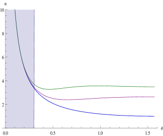
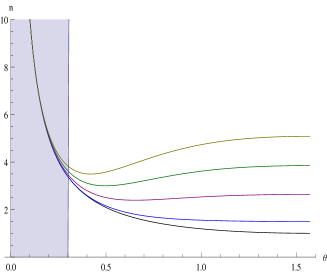
Figure 4: The index $n\in{\mathbb{R}}$ for $A^{\mu}_{\parallel}$ as a function of $\theta$. On the left we vary $\alpha=1/137\,(blue),1\,(purple),2\,(green)$ at $\Upsilon=10$; on the right we vary $\Upsilon=5\,(blue),10\,(purple),15\,(green),20\,(yellow)$ at $\alpha=1$. The lower (black) curves are $1/\sin\theta$

$\bullet$ The curves go asymptotically to $\frac{1}{s_{\theta}}$ when $\theta\to 0$. However, we shall see that they should be truncated before $\theta=0$).

$\bullet$ At large angles, the effects are mainly of quantum nature, strongly influenced by the presence of $B$ and largely depending on the value of $\alpha$; when $\theta$ gets smaller, one goes to another regime in which the effects of confinement are the dominant ones. The strict limit $\theta\to 0$ is special (see subsection 5.5).

Quantum 1-loop effects are therefore potentially large at $\alpha\geq 1$. Furthermore, at reasonable values of $B$ and for photons in the visible spectrum, the dependence on $B$ turns out to be strong. The “confinement” of massless Dirac electrons inside a very thin strip of graphene obviously acts as an amplifier of the effects of their interaction with photons in a magnetic background.

$\bullet$ Quantum effects vary inversely to the energy of the photon : low frequencies are favored for testing, and this limit is fortunate since our expansions were done precisely at $\eta=aq_{0}\ll 1$.

$\bullet$ For $\eta\ll 1$ and $n>\frac{1}{s_{\theta}}$, the residues of $V$ at the poles $\sigma_{1}$ and $\sigma_{2}$ are

$$res(\sigma_{1})=-\frac{\eta}{2i\sqrt{n^{2}s^{2}_{\theta}-1}}+{\cal O}(\eta^{2})=-res(\sigma_{2}).$$ (66)

The agreement between $\Re(V)$ in the first line of (61) and $\pm 2i\pi\ res(\sigma_{1})$ is conspicuous. Indeed, it is easy to prove that for $n\in{\mathbb{R}}$, only one of the 2 poles lies inside the contour of integration in the upper 1/2 complex $\sigma$-plane which is the alternate method to calculate $V$.

This confirms that the transmittance function $U$ alone, through its pole(s) is at the origin of the “leading” $\frac{1}{s_{\theta}}$ behavior of the refraction index (see subsection 5.4.6). The poles are nothing more that the ones of the outgoing photon propagator (in the Feynman gauge) $-i\frac{g^{\nu\sigma}}{\hat{q}^{2}-(q^{3}+k_{3})^{2}}$. We recall that $k_{3}$ is the momentum non-conservation along $B$, which is related (bounded by) to the momentum allowed by quantum mechanics to electrons confined into a strip of thickness $2a$. The non-trivial poles of $U$ (or $V$) and the leading behavior of the refraction index therefore originate from the sole interactions of photons with “confined” electrons.

$\bullet$ In the approximation that we made, the refractive index does not depends on $u$, the position inside the strip. This dependence, very weak, only starts to appear through higher orders in the expansion of the transmittance $U$ (or $V$).

5.4.6 The “leading” $\boldsymbol{n\sim\frac{1}{\sin\theta}}$ behavior

It is easy to track the origin of the leading $\frac{1}{s_{\theta}}$ behavior of the index (we shall see below that the associated divergence at $\theta\to 0$ is fake).

It comes in the regime when the 2 poles of $V$ lie in different 1/2 planes, such that $V$ can be safely approximated by $V\approx 2i\pi\;residue(\sigma_{1}\ or\ \sigma_{2})$.

Keeping only the leading terms in the light-cone equation (58) and using (66) gives then

$$1-\frac{\alpha}{\pi^{2}}\frac{\zeta}{\eta^{2}}\left(2i\pi\frac{\eta}{2i\sqrt{n^{2}s^{2}_{\theta}-1}}\right)=0,$$ (67)

which yields

$$n^{2}s^{2}_{\theta}-1\sim\left(\frac{\alpha s^{2}_{\theta}\Upsilon}{\pi}\right)^{2}.$$ (68)

The $\frac{1}{s_{\theta}}$ leading behavior of the index is therefore associated with the transmittance $V$ and is of “geometric” origin (shape of the sample, localization of the interaction vertices inside the graphene strip). This gets confirmed in section 6 where a similar study is done in the absence of any external $B$: only the $\frac{1}{s_{\theta}}$ behavior of the index is then practically left over.

5.5 The transition $\boldsymbol{\theta\to 0}$

It is fairly easy to determine the value of $\theta$ below which our calculations and the resulting approximate formula (65) may not be trusted anymore. There presumably starts a transition to another regime.

Our calculations stay valid as long as the 2 poles $\sigma_{1}$ and $\sigma_{2}$ of the transmittance function $V$ lie in different 1/2 planes. This requires that their imaginary parts have opposite signs. Their explicit expressions are given in (86) below. It is then straightforward to get the following condition

$$\sigma_{1}\ \text{and}\ \sigma_{2}\ \text{in different 1/2 planes}\Leftrightarrow n_{1}^{2}>\frac{1+n_{2}^{2}}{\tan^{2}\theta}.$$ (69)

(69) is always satisfied at $\theta=\frac{\pi}{2}$ and never at $\theta=0$. Since $n_{2}\approx 0$, the transition occurs at

$$n_{1}(\theta)\approx n(\theta)\approx\frac{1}{\tan\theta},$$ (70)

in which we can use (65) for $n$. Since at small $\theta$, $\sin\theta\simeq\theta\simeq\tan\theta$, this condition writes approximately

$$1\leq\frac{1+\left(\frac{\alpha\Upsilon s_{\theta}^{2}}{\pi}\right)^{2}\left(1+\frac{1}{2\Upsilon^{2}}\right)}{1+2\left(\frac{\alpha s_{\theta}}{\pi}\right)^{2}(3s^{2}_{\theta}+c^{2}_{\theta})}\Leftrightarrow\theta\geq\theta_{min}=\sqrt{\frac{2}{\Upsilon^{2}-\frac{7}{2}}}.$$ (71)

For example, at $\Upsilon=5$ it yields $\theta\geq.3$. Notice that the condition (71) also sets a lower limit $\Upsilon>\sqrt{\frac{7}{2}}$.

It is easy to get the value $n_{max}$ of $n$ at $\theta=\theta_{min}\simeq\frac{\sqrt{2}}{\Upsilon}$ given by (71). Plugging this value in (65) one gets

$$n_{max}\equiv n(\theta=\theta_{min})\approx\frac{\Upsilon}{\sqrt{2}}.$$ (72)

Seemingly, the solution (65) that we have exhibited gets closer and closer to the “leading” $\frac{1}{s_{\theta}}$ when $\theta$ becomes smaller and smaller. The easiest way to show that this divergent is fake relies on a physical argument: the poles of the outgoing photon propagator, which are also those of the transmittance $U$ should be such that $|k_{3}|$, the momentum exchanged with electrons along $B$ is smaller or equal than $\frac{1}{a}=p_{3}^{m}$, which is the maximum quantum momentum of the confined electrons of graphene. Mathematically, this traduces for the poles (59) of $V$ by

$$|\sigma_{1}|\leq 1,\quad|\sigma_{2}|\leq 1.$$ (73)

For $n>\frac{1}{s_{\theta}}$, both conditions yield

$$n^{2}\leq n^{2}_{quant}=\frac{1}{\eta^{2}}+1.$$ (74)

Remark that $n_{max}$ is much smaller than the quantum limit (74).

The case $\theta=0$ is special and is investigated directly. One has then $\sigma_{1}=-\eta(n-1),\sigma_{2}=-\eta(n+1)$, such that $|\sigma_{1}|,|\sigma_{2}|\leq 1$, that is

$$n(\theta=0)\stackrel{{\scriptstyle quantum}}{{\leq}}\frac{1}{\eta}-1.$$ (75)

For finite $\eta$, this bound does not diverge, which shows that the diverging solution (65) cannot be relied on down to $\theta=0$. It can be trusted at most down to a value of $\theta$ for which $n^{2}=n^{2}_{quant}$. Therefore, if a solution exists at $\theta=0$, $n$ must cross the curve $n=\frac{1}{s_{\theta}}$ somewhere at small $\theta$.

However, as we now argue, such a transition cannot exist. This is most easily proved by showing that, at no value of $\theta$, $n=\frac{1}{s_{\theta}}$ can be a solution to the light-cone equation (58). Let us write $\sigma_{1}=-\eta\frac{c_{\theta}}{s_{\theta}}+\epsilon,\sigma_{2}=-\eta\frac{c_{\theta}}{s_{\theta}}-\epsilon$. The poles being real, $V$ can be calculated by setting $\Theta(0)=\frac{1}{2}$ in (60), which yields

$$\begin{split}V&\stackrel{{\scriptstyle real\ poles}}{{\rightarrow}}-\frac{\pi\eta^{2}}{\sigma_{1}\sigma_{2}(\sigma_{1}-\sigma_{2})}\left(\sigma_{1}-\sigma_{2}+\sigma_{2}\cos\sigma_{1}e^{i\sigma_{1}u}-\sigma_{1}\cos\sigma_{2}e^{i\sigma_{2}u}\right)\cr&\hskip-28.45274pt=-\frac{\pi\eta^{2}}{\sigma_{1}\sigma_{2}(\sigma_{1}-\sigma_{2})}\Big{(}\sigma_{1}-\sigma_{2}+\sigma_{2}\cos\sigma_{1}\cos u\sigma_{1}-\sigma_{1}\cos\sigma_{2}\cos u\sigma_{2}+i\big{(}\sigma_{2}\cos\sigma_{1}\sin u\sigma_{1}-\sigma_{1}\cos\sigma_{2}\sin u\sigma_{2}\big{)}\Big{)}.\end{split}$$ (76)

and, in our case, at $u=0$,

$$V(u=0)\approx-\pi\frac{s^{2}_{\theta}}{c^{2}_{\theta}}\left(1-\cos(\eta^{2}\frac{c^{2}_{\theta}}{s^{2}_{\theta}})-\eta\frac{c_{\theta}}{s_{\theta}}\sin(\eta\frac{c_{\theta}}{s_{\theta}})\right).$$ (77)

The light-cone equation (58) for $A^{\mu}_{\parallel}$ writes then

$$\left(1-\frac{1}{s^{2}_{\theta}}\right)\left[1+\frac{\alpha}{\pi}\frac{s^{2}_{\theta}}{c^{2}_{\theta}}\frac{1}{\zeta}\left(c^{2}_{\theta}-\Upsilon^{2}s^{2}_{\theta}(1-\frac{2}{\Upsilon^{2}})\right)\left(1-\cos(\eta^{2}\frac{c^{2}_{\theta}}{s^{2}_{\theta}})-\eta\frac{c_{\theta}}{s_{\theta}}\sin(\eta\frac{c_{\theta}}{s_{\theta}})\right)\right]=0,$$ (78)

in which we have incorporated the “trivial” term $(1-n^{2})$.

Eq. (78) has no solution: the crossing that would make the connection between our diverging solution and an hypothetical solution in the domain lying below the absolute quantum bound (74) cannot be realized . Hence, the domain in which we can trust our solution (65) cannot be extended down to $\theta=0$ .

Does graphene become “opaque” to photons (total reflection) at very small $\theta$, or is this the sign that, for more and more energetic photons and larger and larger external magnetic fields, the simple model that we made for graphene is no longer valid? We cannot decide in the framework of this limited study. “Something may happen” to photons below a certain angle of incidence, but we must also keep in mind that we only used an expansion of the vacuum polarization dangerously truncated to 1-loop in a situation where $\alpha\simeq 2$.

This investigation will be continued in subsection 5.8.2 for $n\in{\mathbb{C}}$ (see also the concluding subsection 7.2).

5.6 The quantum upper bound $\boldsymbol{n<n_{quant}}$. The threshold at $\boldsymbol{B=B^{m}}$

We have seen in (74) that Quantum Mechanics sets an upper bound $n_{quant}$ for the index. It is a large value for optical frequencies but, when the energy of photons $q_{0}=\frac{\eta}{a}$ increases, $n_{quant}$ decreases accordingly, its asymptotic value being $1$ for infinitely energetic photons.

Our calculations being only valid at large $\Upsilon\equiv\frac{\sqrt{2eB}}{q_{0}}\gg 1$, harder and harder photons need larger and larger values of $B$ (that probably cannot be realized on earth). Then, $\theta_{min}$ given in (71) also decreases, while $n_{max}\equiv n(\theta_{min})$ given by (72) increases. A point can be reached at which $n_{max}$ becomes equal, then larger than $n_{quant}$. $n_{max}\sim n_{quant}$ occurs at $\eta\simeq\frac{\sqrt{2}}{\Upsilon}\Leftrightarrow\zeta\simeq\sqrt{2}$, independently of $\eta$. It corresponds (see subsection 5.1) to $B\simeq B^{m}\approx 21531\,T$. $B^{m}$ appears therefore as the (very large) magnetic field at which the two upper bounds $n_{max}$ and $n_{quant}$ coincide. Still increasing $B$ would result in $n_{max}$ exceeding the quantum limit, which is impossible. So, new phenomena are expected for $B>B^{m}$, which lie beyond the scope of this work.

5.7 Reliability of the approximation $\boldsymbol{F(x)\approx\frac{1}{1-x}}$ for the electron propagator

The approximation (21) that we made for the expression of the electron propagator inside graphene (see subsection 3.1.2) is only valid for low energy electrons with $p_{0}\leq 1.2\sqrt{2eB}$. Using subsection 5.1 for the orders of magnitude, the lowest external magnetic field $B=1\,T$ that we consider corresponds to $\zeta\approx\frac{1}{100}$ and therefore to an energy $\approx\sqrt{2}\,\frac{1}{100}\,10^{-3}m_{e}\approx 7\,eV$. Accordingly, our approximation is reliable for electrons with energy $p_{0}\leq 10\,eV$. This is satisfied inside graphene.

Note that the visible light that we send through graphene has also energy $\leq 3.5\,eV$.

5.8 Going to $\boldsymbol{n\in{\mathbb{C}}}$

5.8.1 The case of $\boldsymbol{A^{\mu}_{\parallel}}$

Numerical calculations can be performed in the general case of a complex index $n=n_{1}+in_{2}$. They show in particular that $|n_{2}|\ll n_{1}$, confirming the reliability of the approximation that we made in the main stream of this study (we have limited them to values of $\theta$ large enough for our equations to be valid). The results are displayed on Fig.5, in which we plot $n_{2}$ as a function of $\theta$, varying $\alpha$ (left) and $\Upsilon$ (right), and on Fig.6 in which we plot $n_{2}$ as a function of $u$, varying $\Upsilon$.

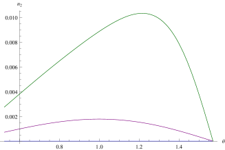
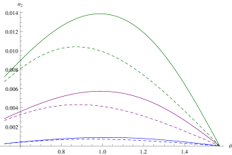
Figure 5: The imaginary part $n_{2}$ of the index $n$ for $A^{\mu}_{\parallel}$ as a function of $\theta$. On the left we vary $\alpha=1/137\,(blue)$, $1\,(purple)$, $2\,(green)$ at $\Upsilon=5$; on the right we vary $\Upsilon=4\,(blue)$, $8\,(purple)$, $12\,(green)$ at $\alpha=1$. The dashed curves on the right correspond to the rough approximation (81)

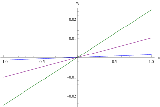
Figure 6: The imaginary part $n_{2}$ of index $n$ for $A^{\mu}_{\parallel}$ as a function of $u$. We take $\alpha=1$, $\eta=5/1000$, and vary $\Upsilon=4\,(blue),8\,(purple),12\,(green)$

To this purpose, and because the real part of the light-cone equation only gets very slightly modified, it is enough to consider the imaginary part of the light-cone equation (58) for $A^{\mu}_{\parallel}$ in which we plug, for $n_{1}^{2}$, the analytic expression (65). In practice, the expansion of this equation at ${\cal O}(\eta^{2})$ and ${\cal O}(n_{2})$, which is a polynomial of first order in $n_{2}$ is enough for our purposes An important ingredient of the calculation is the expansion of the transmittance $V$ at order ${\cal O}(\eta^{2})$ and ${\cal O}(n_{2})$, in the case when its 2 poles lie in different 1/2 planes, which writes

$$\begin{split}\frac{1}{\pi}\Re(V)&=-\frac{\eta}{\sqrt{n_{1}^{2}s^{2}_{\theta}-1}}+\frac{1}{2}(1+u^{2})\eta^{2}+\frac{uc_{\theta}(2n_{1}^{2}s^{2}_{\theta}-1)}{(n_{1}^{2}s^{2}_{\theta}-1)^{\frac{3}{2}}}\eta^{2}n_{2}+\ldots,\cr\frac{1}{\pi}\Im(V)&=\frac{un_{1}c_{\theta}}{\sqrt{n_{1}^{2}s^{2}_{\theta}-1}}\eta^{2}-\frac{n_{1}s^{2}_{\theta}}{(n_{1}^{2}s^{2}_{\theta}-1)^{\frac{3}{2}}}\eta n_{2}+\ldots\end{split}$$ (79)

The corresponding analytical expression for $n_{2}$, an odd function of $u$, is long and unaesthetic and we only give it in footnote 12 . However a rough order of magnitude can be obtained with very drastic approximations which lead to the equation

$$n_{2}s^{2}_{\theta}\sim u\eta c_{\theta}(n_{1}^{2}s_{\theta}^{2}-1),$$ (81)

in which, like before, we can plug in the analytical formula (65) for $n_{1}^{2}$. The corresponding curves are the dashed ones in Fig.5 .

As $B$ increases, it is no longer a reliable approximation to consider the index to be real : absorption becomes non-negligible. The window of medium-strong $B$’s from 1 to 20 Teslas together with photons in the visible range appears therefore quite simple and special. Outside this window, the physics is most probably much more involved and equations much harder to solve.

5.8.2 The “wall” for $\boldsymbol{A^{\mu}_{\parallel}}$

The situation is best described in the complex $(n_{1},n_{2})$ plane of the solutions $n=n_{1}+in_{2}$ of the light-cone equation (58) for $A^{\mu}_{\parallel}$, which decomposes into its real and imaginary parts (in the limit $\eta\ll\zeta\Leftrightarrow\Upsilon\gg 1$, and neglecting the exponential $e^{-\frac{n^{2}s^{2}_{\theta}}{\Upsilon^{2}}}$ which plays a negligible role) according to

$$\begin{split}&\ast\ 1+\frac{\alpha}{\pi}\frac{s^{2}_{\theta}}{\zeta}\left(1+\frac{1}{4\Upsilon^{2}}\right)\left[\left(\Upsilon^{2}-(n_{1}^{2}-n_{2}^{2})(1+s^{2}_{\theta})\right)\Re(V)+2n_{1}n_{2}(1+s^{2}_{\theta})\Im(V)\right]=0,\cr&\ast\ -2n_{1}n_{2}(1+s^{2}_{\theta})\Re(V)+\left(\Upsilon^{2}-(n_{1}^{2}-n_{2}^{2})(1+s^{2}_{\theta}\right)\Im(V)=0.\end{split}$$ (82)

All previous calculations favoring solutions with low absorption $|n_{2}|\ll n_{1}$, it is in this regime that we shall investigate the presence of a “wall” at small $\theta$. To this purpose, we shall plug into the light-cone equation (58) for $A^{\mu}_{\parallel}$ the expansion of the transmittance $V$ that is written in (79).

The situation at $\theta=\frac{\pi}{4}$ (left) and $\theta=\frac{\pi}{10}$ are depicted in Fig.7. The values of the parameters are $\alpha=1,u=.5,\eta=\frac{5}{1000},\Upsilon=5$.

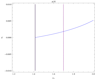
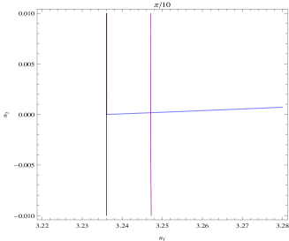
Figure 7: The index $(n_{1},n_{2})$ for $A^{\mu}_{\parallel}$ at $\theta=\frac{\pi}{4}$ (left) and $\theta=\frac{\pi}{10}$ (right)

The purple curve corresponds to the solutions of the real part of the light-cone equation and the blue quasi-vertical line to the solution of its real part. The intersection of the 2 curves yields the solution $n=n_{1}+in_{2}$. We recover $|n_{2}|\ll n_{1}$. The black vertical line on the left corresponds to $n_{1}=\frac{1}{s_{\theta}}$.

A transition brutally occurs close to $\theta=\frac{\pi}{14}$. Then the solution at $|n_{2}|\ll n_{1}={\cal O}(1)$ disappears. It is clearly visible on Fig.8 below in which we plot the situation after the transition, for $\theta=\frac{\pi}{17}$.

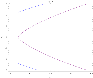
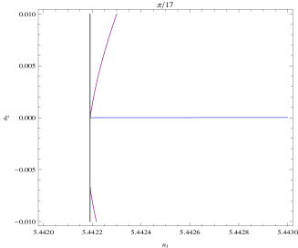
Figure 8: The index $(n_{1},n_{2})$ for $A^{\mu}_{\parallel}$ at $\theta=\frac{\pi}{17}$. The right figure is an enlargement of the left one

There is no more intersection between the solutions of the real (purple) and imaginary (blue) parts of the light-cone equations, except at $n_{2}=0,n_{1}=\frac{1}{s_{\theta}}$, which is a fake solution since we know that $n_{1}$ can never reach its “asymptotic” value $\frac{1}{s_{\theta}}$.

5.8.3 An estimate of the angle of transition $\boldsymbol{\theta_{min}}$

This change of regime is characterized by a brutal jump in the value of $n_{2}$, which should be manifest on the imaginary part of the light-cone equation (82). A very reliable approximation can be obtained by truncating $\Re(V)$ to its first term, in which case one gets

$$n_{2}\approx(n_{1}^{2}s^{2}_{\theta}-1)\frac{u\eta c_{\theta}\left(\Upsilon^{2}-n_{1}^{2}(1+s^{2}_{\theta})\right)}{s^{2}_{\theta}\left(\Upsilon^{2}-n_{1}^{2}(1+s^{2}_{\theta})\right)-2(1+s^{2}_{\theta})(n_{1}^{2}s^{2}_{\theta}-1)}$$ (83)

which has a pole at (we use $s^{2}_{\theta}\ll 1$)

$$n_{1}^{2}\approx\frac{2+\Upsilon^{2}s^{2}_{\theta}}{3s^{2}_{\theta}}.$$ (84)

This value for $n_{1}$ determines the maximum that can be reached when $\theta$ decreases. Indeed, then, $n_{2}$ becomes out of control in the framework of our approximations. We also know that that $n_{1}$ should stay below $\frac{1}{s_{\theta}}$. The intersection of (84) and $\frac{1}{s_{\theta}}$ yields the lower limit for $\theta$

$$\theta_{min}\sim\frac{1}{\Upsilon}.$$ (85)

(85) is smaller than our previous estimate (71) obtained in the approximation $n\in{\mathbb{R}}$.

At $\Upsilon=5$ one gets $\theta_{min}\approx\frac{\pi}{15}$, which shows the reliability of our estimate (the true transition numerically occurs between $\frac{\pi}{14}$ and $\frac{\pi}{15}$).

5.8.4 The case of $\boldsymbol{A^{\mu}_{\perp}}$

We only summarize below the steps that lead to the conclusion that no solution to the refraction index except the trivial $n=1$ exists for the transverse polarization.

Starting from the corresponding light-cone equation in (58), the main task is to get the appropriate expression for the transmittance function $V$. To this purpose the starting point is the general expression (60). We expand it in powers of $\eta$ in the sense that the exponentials are expanded at ${\cal O}(\eta)$ or, eventually ${\cal O}(\eta^{2})$. No expansion in powers of $n_{2}$ is done because, if solutions exist, they may occur for fairly larges values of $n_{2}$ (and $n_{1}$).

Since the sign of the imaginary parts of the poles $\sigma_{1}$ and $\sigma_{2}$ obviously play a central role, it is also useful to extract

$$\begin{split}\Im(\sigma_{1})&=\eta\left(-n_{2}c_{\theta}+\frac{1}{\sqrt{2}}\sqrt{-c+\sqrt{c^{2}+d^{2}}}\right),\cr\Im(\sigma_{2})&=\eta\left(-n_{2}c_{\theta}-\frac{1}{\sqrt{2}}\sqrt{-c+\sqrt{c^{2}+d^{2}}}\right),\cr c&=1-(n_{1}^{2}-n_{2}^{2})s^{2}_{\theta},\quad d=2n_{1}n_{2}s^{2}_{\theta}.\end{split}$$ (86)

Straightforward manipulations on (60) show that:

* when $n_{2}>0$ ($\Rightarrow\Im(\sigma_{2})<0$): if $\Im(\sigma_{1})>0$, $V=\frac{-i\pi\eta}{\sqrt{1-n^{2}s^{2}_{\theta}}}+\ldots$; if $\Im(\sigma_{1})<0$, $V=\frac{\pi\eta^{2}}{2}(1-u)^{2}+\ldots$
* when $n_{2}<0$ ($\Rightarrow\Im(\sigma_{1})>0$): if $\Im(\sigma_{2})>0$, $V=\frac{\pi\eta^{2}}{2}(1+u)^{2}+\ldots$; if $\Im(\sigma_{2})<0$, $V=\frac{-i\pi\eta}{\sqrt{1-n^{2}s^{2}_{\theta}}}+\ldots$

The cases when $V={\cal O}(\eta^{2})$ correspond to $\sigma_{1}$ and $\sigma_{2}$ being in the same 1/2 complex $\sigma$-plane.

When $V=\frac{-i\pi\eta}{\sqrt{1-n^{2}s^{2}_{\theta}}}$, its real and imaginary parts are given by

$$\Re(V)=\frac{\pi\eta n_{1}n_{2}s^{2}_{\theta}}{\sqrt{2}}\frac{\sqrt{c+\sqrt{c^{2}+d^{2}}}}{\sqrt{c^{2}+d^{2}}},\qquad\Im(V)=\frac{-\pi\eta}{\sqrt{2}}\frac{\sqrt{-c+\sqrt{c^{2}+d^{2}}}}{\sqrt{c^{2}+d^{2}}}.$$ (87)

Numerical solutions of the light-cone equation show that no solution exists that fulfill the appropriate criteria on the signs of $\Im(\sigma_{1}),\Im(\sigma_{2})$. For example, for $n_{2}<0$, one gets solutions shared by both the real and imaginary parts of the light-cone equations, but they satisfy $\Im(\sigma_{2})>0$ and must therefore be rejected.

The next step is to use the exact expression (60) of $V$, but no acceptable solution exists (solutions with very large values of $n_{1}$ and $n_{2}$, larger than $20$, are a priori rejected).

6 The case $\boldsymbol{B=0}$

6.1 The vacuum polarization $\boldsymbol{\Pi^{\mu\nu}}$

Standard techniques applied to massless electrons of graphene at the Dirac point lead to the exact results

$$\begin{split}i\Pi^{11}_{\xcancel{B}}(\hat{q})&=i\frac{e^{2}}{8}\left(\sqrt{\hat{q}_{E}^{2}}-\frac{q_{1}^{2}}{\sqrt{\hat{q}_{E}^{2}}}\right),\cr i\Pi^{22}_{\xcancel{B}}(\hat{q})&=i\frac{e^{2}}{8}\left(\sqrt{\hat{q}_{E}^{2}}-\frac{q_{2}^{2}}{\sqrt{\hat{q}_{E}^{2}}}\right),\cr i\Pi^{33}_{\xcancel{B}}&=i\frac{e^{2}}{4}\sqrt{\hat{q}_{E}^{2}},\cr i\Pi^{00}_{\xcancel{B}}&=-i\frac{e^{2}}{8}\frac{q_{1}^{2}+q_{2}^{2}}{\sqrt{\hat{q}_{E}^{2}}},\cr i\Pi^{12}_{\xcancel{B}}&=-i\frac{e^{2}}{8}\frac{q_{1}q_{2}}{\sqrt{\hat{q}_{E}^{2}}},\cr i\Pi^{01}_{\xcancel{B}}&=-\frac{e^{2}}{8}\frac{q_{0}^{E}q_{1}}{\sqrt{\hat{q}_{E}^{2}}},\cr i\Pi^{02}_{\xcancel{B}}&=-\frac{e^{2}}{8}\frac{q_{0}^{E}q_{2}}{\sqrt{\hat{q}_{E}^{2}}},\cr&\Pi^{03}_{\xcancel{B}}=\Pi^{13}_{\xcancel{B}}=\Pi^{23}_{\xcancel{B}}=0.\end{split}$$ (88)

in which $q_{0}=iq_{0}^{E}$ and $(\hat{q}^{E})^{2}=(q_{0}^{E})^{2}+q_{1}^{2}+q_{2}^{2}$.

$\star$ $\Pi^{ij}_{\xcancel{B}}$ is proportional to $\pi\alpha$ while, in the presence of $B$, it was proportional to $\alpha$. The extra $\pi$ comes from $\int_{0}^{1}dx\;\sqrt{x(1-x)}=\frac{\pi}{8}$.

$\star$ Transversality: one easily checks on (88) that $q_{0}\Pi^{00}_{\xcancel{B}}+q_{1}\Pi^{10}_{\xcancel{B}}+q_{2}\Pi^{20}_{\xcancel{B}}=0$, $q_{0}\Pi^{01}_{\xcancel{B}}+q_{1}\Pi^{11}_{\xcancel{B}}+q_{2}\Pi^{21}_{\xcancel{B}}=0$, $q_{0}\Pi^{02}_{\xcancel{B}}+q_{1}\Pi^{12}_{\xcancel{B}}+q_{2}\Pi^{22}_{\xcancel{B}}=0$. The last condition $q_{0}\Pi^{03}_{\xcancel{B}}+q_{1}\Pi^{13}_{\xcancel{B}}+q_{2}\Pi^{23}_{\xcancel{B}}+q_{3}\Pi^{33}_{\xcancel{B}}=0$ reduces to $q_{3}\Pi^{33}_{\xcancel{B}}=0$, which is not satisfied unless $q_{3}=0$ or $\hat{q}_{E}^{2}=0$ (“on mass shell 2+1 photon”).

In our setup, we recall $n^{2}=\frac{q_{1}^{2}+\xcancel{q_{2}^{2}}+q_{3}^{2}}{q_{0}^{2}}$, $n_{x}=\frac{q_{1}}{q_{0}}=ns_{\theta},n_{z}=\frac{q_{3}}{q_{0}}=nc_{\theta}$. One has $(\hat{q}_{E})^{2}=(q_{0}^{E})^{2}+q_{1}^{2}+q_{2}^{2}=q_{0}^{2}(n^{2}s^{2}_{\theta}-1)$ because $q_{2}=0$. So, $\sqrt{\hat{q}_{E}^{2}}=\pm q_{0}\sqrt{n^{2}s^{2}_{\theta}-1}$. This gives

$$\begin{split}\Pi^{11}_{\xcancel{B}}&=\mp\frac{\pi\,\alpha}{2}q_{0}\frac{1}{\sqrt{n^{2}s^{2}_{\theta}-1}},\cr\Pi^{22}_{\xcancel{B}}&=\pm\frac{\pi\,\alpha}{2}q_{0}\sqrt{n^{2}s^{2}_{\theta}-1},\cr\Pi^{33}_{\xcancel{B}}&=\pm\pi\,\alpha\,q_{0}\sqrt{n^{2}s^{2}_{\theta}-1},\cr\Pi^{00}_{\xcancel{B}}&=\mp\frac{\pi\,\alpha}{2}q_{0}\frac{n^{2}s^{2}_{\theta}}{\sqrt{n^{2}s^{2}_{\theta}-1}},\cr\Pi^{12}_{\xcancel{B}}&=0,\quad\Pi^{i3}_{\xcancel{B}}=0,\cr\Pi^{01}_{\xcancel{B}}&=\pm\frac{\pi\alpha}{2}q_{1}\frac{1}{\sqrt{n^{2}s^{2}_{\theta}-1}},\cr\Pi^{02}_{\xcancel{B}}&=\pm\frac{\pi\alpha}{2}q_{2}\frac{1}{\sqrt{n^{2}s^{2}_{\theta}-1}}.\end{split}$$ (89)

6.2 The light-cone equation and the refractive index

The light-cone equations (57) together with (89) yield

$$\begin{split}&for\ A^{\mu}_{\perp}:(1-n^{2})\left[1\pm\frac{\alpha}{\eta}\sqrt{n^{2}s^{2}_{\theta}-1}\;\frac{V(u,\rho,n,\theta,\eta)}{\pi}\right]=0,\cr&for\ A^{\mu}_{\parallel}:(1-n^{2})\left[1\pm\frac{\alpha}{\eta}\Big{(}-\frac{c^{2}_{\theta}}{2\sqrt{n^{2}s^{2}_{\theta}-1}}+s^{2}_{\theta}\sqrt{n^{2}s^{2}_{\theta}-1}\Big{)}\;\frac{V(u,\rho,n,\theta,\eta)}{\pi}\right]=0.\end{split}$$ (90)

in which $V$ is the same transmittance function as before, given by (52).

6.3 Solutions for $\boldsymbol{A^{\mu}_{\parallel}}$ with $\boldsymbol{n\in{\mathbb{R}}}$

We approximate, at $\eta\ll 1$, according to (61), $V\approx-\frac{\eta\pi}{\sqrt{n^{2}s^{2}_{\theta}-1}}$.

Like in the presence of $B$, no non-trivial solution exists for the transverse polarization and we focus hereafter on $A^{\mu}_{\parallel}$. The corresponding light-cone equation writes

$$1\pm\alpha\left(-\frac{c_{\theta}^{2}}{2(n^{2}s_{\theta}^{2}-1)}+s^{2}_{\theta}\right)=0,$$ (91)

(91) has seemingly 2 types of solutions, the first with $n>\frac{1}{s_{\theta}}$ and the second with $n<\frac{1}{s_{\theta}}$. They write respectively

$$\begin{split}&\ast\ n>\frac{1}{s_{\theta}}:n^{2}=\frac{1}{s_{\theta}^{2}}\left(1+\frac{\alpha c_{\theta}^{2}}{2(1+\alpha s_{\theta}^{2})}\right),\cr&\ast\ n<\frac{1}{s_{\theta}}:n^{2}=\frac{1}{s^{2}_{\theta}}\left(1-\frac{\alpha c^{2}_{\theta}}{2(1-\alpha s^{2}_{\theta})}\right).\end{split}$$ (92)

They are plotted on Fig.9, respectively on the left for $n>\frac{1}{s_{\theta}}$ and on the right for $n<\frac{1}{s_{\theta}}$. They only depend on $\alpha$ and we plot them for $\alpha=\frac{1}{137}$ (blue), $\alpha=1$ (purple) and $\alpha=1.5$ (green), $\alpha=2$ (yellow) together with $n=\frac{1}{s_{\theta}}$ (black), the latter being in practice indistinguishable from $\alpha=\frac{1}{137}$.

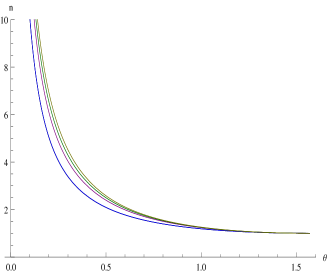
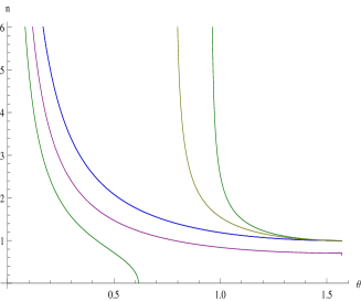
Figure 9: The 2 types of real solutions of the light-cone equation for $A^{\mu}_{\parallel}$ as a function of $\theta$ when no external $B$ is present. On the left $n>\frac{1}{s_{\theta}}$, on the right $n<\frac{1}{s_{\theta}}$. We vary $\alpha=1/137\;(blue)$, $1\;(purple)$, $1.5\;(green)$, $2\;(yellow)$. The black ($\simeq$ blue) curves are $1/\sin\theta$

Looking at the curves, it is conspicuous that one cannot trust them, neither when $\theta\to 0$ because of divergences, nor when $\theta$ becomes large for $\alpha>1$. In particular, the solution with $n<\frac{1}{s_{\theta}}$ becomes out of control above $\theta\geq.5$; it furthermore cannot exist when $s^{2}_{\theta}>\frac{1}{\alpha}$ since then $n>\frac{1}{s_{\theta}}$ (a divergence occurs at $s^{2}_{\theta}=\frac{1}{\alpha}$).

The approximation of considering $n\in{\mathbb{R}}$ is obviously very hazardous, specially when $\alpha>1$. This is why we shall perform in subsection 6.4 a detailed study with $n\in{\mathbb{C}}$.

6.4 Solutions with $\boldsymbol{n\in{\mathbb{C}}}$

6.4.1 There is no solution with $\boldsymbol{n_{1}<\frac{1}{s_{\theta}}}$

When supposing $n\in{\mathbb{R}}$, we have seen that the solution with $n<\frac{1}{s_{\theta}}$ was unstable, in particular above $\theta_{max}$ such that $(\sin\theta_{max})^{2}=\frac{1}{\alpha}$ were it did not exist anymore.

Careful investigations for $n\in{\mathbb{C}}$ show that, like in the presence of $B$, no solution with $n_{1}<\frac{1}{s_{\theta}}$ exists .

6.4.2 The solution with $\boldsymbol{n_{1}>\frac{1}{s_{\theta}}}$

In the presence of an external $B$, we have seen that the solution with a quasi-real index suddenly disappears below an angle $\theta_{min}\approx\frac{1}{\Upsilon}$. In the present case with no external $B$, there is no $\theta_{min}$ but the index becomes “more and more complex” (that is the ratio of its imaginary and real parts increase) when $\theta$ becomes smaller and smaller.

To demonstrate this, we study the light-cone equation (90) for $A^{\mu}_{\parallel}$ with $n=n_{1}+in_{2},\ n_{1},n_{2}\in{\mathbb{R}}$. For practical reasons, we shall limit ourselves to the expansion of $V$ at small $\eta$ and $n_{2}$, valid when the 2 poles of $V$ lie in different 1/2 planes, given in (79).

Calling

$$c=(n_{1}^{2}-n_{2}^{2})s^{2}_{\theta}-1,\quad d=-2n_{1}n_{2}s^{2}_{\theta},$$ (94)

the non-trivial parts of the real and imaginary parts of this light-cone equation write (we have chosen the appropriate sign in (90, the one that gives solutions)

$$\begin{split}&1+\frac{\alpha}{\eta\pi}\left[\left(-\frac{c^{2}_{\theta}}{2}\frac{d}{\sqrt{2}\sqrt{c^{2}+d^{2}}\sqrt{-c+\sqrt{c^{2}+d^{2}}}}+s^{2}_{\theta}\frac{-d}{\sqrt{2}\sqrt{-c+\sqrt{c^{2}+d^{2}}}}\right)\Re(V)\right.\cr&\hskip 28.45274pt\left.-\left(-\frac{c^{2}_{\theta}}{2}\frac{\sqrt{-c+\sqrt{c^{2}+d^{2}}}}{\sqrt{2}\sqrt{c^{2}+d^{2}}}+s^{2}_{\theta}\frac{\sqrt{-c+\sqrt{c^{2}+d^{2}}}}{\sqrt{2}}\right)\Im(V)\right]=0,\cr&\left(-\frac{c^{2}_{\theta}}{2}\frac{d}{\sqrt{2}\sqrt{c^{2}+d^{2}}\sqrt{-c+\sqrt{c^{2}+d^{2}}}}+s^{2}_{\theta}\frac{-d}{\sqrt{2}\sqrt{-c+\sqrt{c^{2}+d^{2}}}}\right)\Im(V)\cr&\hskip 28.45274pt+\left(-\frac{c^{2}_{\theta}}{2}\frac{\sqrt{-c+\sqrt{c^{2}+d^{2}}}}{\sqrt{2}\sqrt{c^{2}+d^{2}}}+s^{2}_{\theta}\frac{\sqrt{-c+\sqrt{c^{2}+d^{2}}}}{\sqrt{2}}\right)\Re(V)=0.\end{split}$$ (95)

The results are displayed in Fig.10 below, for $\alpha=1$ (blue), $\alpha=1.5$ (purple) and $\alpha=2$ (green). The values of $n_{1}$ are plotted on the left and the ones of $n_{2}$ on the right. The value of the other parameters are $u=.5,\eta=\frac{5}{1000}$. For $\alpha=\frac{1}{137}$, $n_{1}$ is indistinguishable from $\frac{1}{s_{\theta}}$.

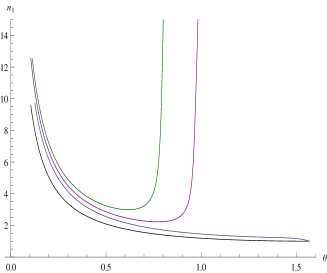
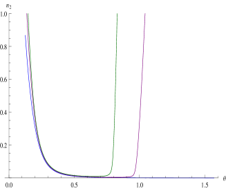
Figure 10: The real part $n_{1}$ (left) and imaginary part $n_{2}$ (right) of the solution $n$ of the light-cone equation (90) for $A^{\mu}_{\parallel}$ in the absence of external $B$. The blue curves correspond to $\alpha=1$, the purple curves to $\alpha=1.5$ and the green curves to $\alpha=2$. The black curve on the left is $n_{1}=\frac{1}{s_{\theta}}$

$\bullet$ As $\theta$ gets smaller and smaller, the index becomes complex with larger and larger values of both its components. It is of course bounded as before to $|n|<\frac{1}{\eta}$ by quantum considerations. The brutal transition at $\theta_{min}\simeq\frac{1}{\Upsilon}$ is replaced by a smooth transition (which could be anticipated since, in the absence of $B$, the parameter $\Upsilon$ does not exist).

$\bullet$ A new feature seems to occur, the presence of a “wall” at large $\theta$ for $\alpha>1$, obviously reminiscent of the divergence that occurred in the approximation $n\in{\mathbb{R}}$ at $\theta=\theta_{max},(\sin\theta_{max})^{2}=\frac{1}{\alpha}$ for the solution $n<\frac{1}{s_{\theta}}$ (we had noticed that this condition could no longer be satisfied since, for $s^{2}_{\theta}>\frac{1}{\alpha}$, $n$ could only be larger than $\frac{1}{s_{\theta}}$).

Three explanations come to the mind concerning this wall. The first is that, for large values of $n_{2}$, the expansion (79) that we used for $V$ is no longer valid; however, using the exact expression for the transmittance leads to the same conclusion. The second, and also very likely one, is that the perturbative series has no meaning whatsoever for $\alpha>1$ (2-loop corrections become larger than 1-loop etc ); using a 2-loop calculation of the vacuum polarization without external $B$ seems feasible but also goes beyond the scope of this work. The third is that this divergence is the sign that some physical phenomenon occurs, like total reflexion, for $\theta>\theta_{max}$, which can only be settled by experiment.

$\bullet$ These calculations show in which domain the approximation $n\in{\mathbb{R}}$ is reliable since it requires $n_{2}\ll 1$: for example $n_{2}<.1$ needs $.3\leq\theta\leq\theta_{max}$, which leaves (except for $\alpha\leq 1$ in which case $\theta_{max}\geq\frac{\pi}{2}$) only a small domain for $\theta$.

$\bullet$ A very weak dependence on $\boldsymbol{\alpha}$ for $\boldsymbol{\theta<\theta_{max}}$

In the absence of external $B$ and away from the “wall” at large $\theta$, the index is seen to depend very little on $\alpha$. The dependence of $n$ on $\theta$ is practically only due to the transmittance function $V$ and to the confinement of electrons inside graphene. Notice in particular that, when $\alpha=\frac{1}{137}\ll 1$, the curve is indistinguishable from that of $\frac{1}{s_{\theta}}$.

The fairly large dependence on $\alpha$ that we uncovered in the presence of $B$ are therefore triggered by $B$ itself.

$\bullet$ The dependence on the energy of the photon

The dependence on $\eta$ only occurs in the imaginary part $n_{2}$ of $n$. This is shown in Fig.11, in which we vary $\eta$ in the visible spectrum, $\eta\in[\frac{2}{1000},\frac{7}{1000}]$ at $\alpha=1.5$ (unlike in Fig.10, $\theta$ has not been extended above $\theta_{max}$).

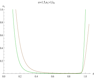
Figure 11: $n_{2}$ as a function of $\theta$ for $\eta=\frac{2}{1000}$ (green) and $\eta=\frac{7}{1000}$ (brown), in the case $\alpha=1.5$

6.5 The limit of very small $\boldsymbol{\theta}$; absorption of visible light and experimental opacity

6.5.1 At small $\boldsymbol{\theta}$

Since absorption of visible light by graphene at close to normal incidence has been measured [11], let us show that our simple model gives predictions that are compatible with these measurements.

To that purpose, we calculated numerically the index $n$ at the lowest value of $\theta$ at which the 2 poles of $V$ lie in different 1/2 planes. We have used the exact expression of $V$ (no expansion) and obtained

$$\begin{split}\ast\ &for\ \alpha=1\ and\ \theta=\frac{\pi}{105.9}:n=41.20+.7\times i,\cr\ast\ &for\ \alpha=2\ and\ \theta=\frac{\pi}{89}:n=40+1\times i.\end{split}$$ (96)

The 2 corresponding angles are small enough to be considered close to normal incidence.

The transmission coefficient along $z$ (therefore for $c_{\theta}\approx 1$) is given by

$$T=e^{-8\pi\eta n_{2}c_{\theta}}\approx 1-8\pi\eta n_{2},$$ (97)

while experimental measurements [11] are compatible with

$$T\approx 1-\pi\,\alpha_{vac},\ \alpha_{vac}=\frac{1}{137}.$$ (98)

This requires

$$n_{2}\approx\frac{\alpha_{vac}}{8\eta}\in[.46,.13]\ for\ \eta\in\left[\frac{2}{1000},\frac{7}{1000}\right].$$ (99)

We get therefore the correct order of magnitude for $n_{2}$. The discrepancy between our prediction and the experimental value can be thought as an estimate of 2-loop corrections in the absence of $B$.

6.5.2 At $\boldsymbol{\theta=0}$

At $\theta=0$, $\vec{q}$ is parallel to the $z$ axis such that there is no more distinction between transverse and parallel polarizations. Since we have found for $\theta\not=0$ no non-trivial solution to the light-cone equation for $A^{\mu}_{\perp}$, but only the trivial one $n=1$, a smooth limit at $\theta=0$, which should be common for the 2 polarizations, would presumably require that, like for $A^{\mu}_{\perp}$, only $n=1$ remains for $A^{\mu}_{\parallel}$, too; but we have yet no proof of this.

So, like in the presence of $B$, we are at a loss to give any prediction at $\theta=0$. This is for sure a limitation of our model.

7 Outlook and prospects

7.1 General remarks

We have shown that the refractive index of graphene in the presence of an external magnetic field is very sensitive to 1-loop quantum corrections. The effects are large for optical wavelengths and even for magnetic fields below 20 Teslas. They only depend (at least for the real part of the refractive index), on the ration $\frac{\sqrt{2eB}}{q_{0}}$ which makes them larger and larger as the photon goes to smaller and smaller energy. We only found them for so-called parallel polarization of the photon. At the opposite, when there is no external $B$, quantum effects stay small and the optical properties of graphene are mainly controlled by the sole transmittance function which incorporates the geometry of the sample and the confinement of electrons along $z$.

By calculating the 1-loop photon propagator in position space, we have been able to localize the interactions of photons with electrons inside graphene, therefore accounting for their “confinement” inside a very thin strip.

One of the main achievements of this study concerns the transmittance function $U$. The optical properties of graphene cannot be indeed deduced by the sole calculation of the genuine vacuum polarization, would it be in “reduced $QED_{4,3}$” [15], because this would in particular neglect all effects due to the confinement of the electron-photon interactions.

The behavior of the refraction index as $\theta$ goes to small values has been shown to depend whether an external $B$ is present or not. When $B\not=0$ there exists a brutal transition at $\theta_{min}\approx\frac{1}{\Upsilon}$ below which the quasi-real solution valid above this threshold disappears, presumably (but this is still to be proved rigorously) in favor of a complex solution with large values of $n_{1}$ and $n_{2}$ (see subsection 7.2). In the absence of $B$ the transition is smooth: $n$ becomes gradually complex with larger and larger values of its real and imaginary components.

Because of the approximations that we have made, and that we list below, we cannot pretend to have devised a fully realistic quantum model. We have indeed:
* truncated the perturbative series at 1-loop;
* truncated the expansion of the electron propagator for large $B$ at next-to-leading order;
* approximated an incomplete $\beta$ function $F(x)=(-2)^{(-1+x)}\beta(-2,1-x,0)\approx\frac{1}{1-x}$, which in particular forget about poles at $p_{0}^{2}=2neB$ except for $n=1$; this is however safe for electrons with energy lower than $7\,eV$, which is certainly the case for graphene through which go photons with energies smaller than $3.5\,eV$;
* chosen a special gauge, the Feynman gauge for the external photons;
* studied light-cone equations only through their expansions at large $\frac{\sqrt{2eB}}{q_{0}}$ and small $aq_{0}$.

We can however reasonably pretend to have gone beyond the brutal limit $B\to\infty$ and to have defined a domain of wavelengths and magnetic fields in which specific expansions and approximations are under control and which are furthermore physically easy to test.

Some comments are due concerning the lack of transversality of the vacuum polarization which arises here, as well as in [10], from the interaction of “quasi-2+1” electrons (in reality 3+1 electrons with $p_{3}$ formally vanishing) with 3+1 photons. Lorentz invariance being explicitly broken, one cannot expect anymore the usual gauge invariance of 3+1 QED to hold like in [7].

A specific choice of gauge appears then less chocking, all the more as it is extremely common when making calculations in condensed matter physics to choose the most convenient (Coulomb or Feynman) gauge.

A tantalizing question concerns of course the magnitude of higher order corrections. If 1-loop corrections to the refraction index are large, how can we trust the result, unless all higher orders are proved to be much smaller? At present we have no answer to this. That $\alpha\simeq 2$ inside graphene is already a bad ingredient for a reliable perturbative treatment and, furthermore, the corrections to $n$ do not look like a standard series in powers of $\alpha$. Comparisons can be made for example with the results obtained in the case of non-confined massive electrons with the effective Euler-Heisenberg Lagrangian [8]. Their equations (2.17)(2.18) show quantum corrections to $n$ proportional to $\alpha\left(\frac{eB}{m_{e}^{2}}\right)^{2}$. In the study of the hydrogen atom [1][2], typical corrections are proportional to $\alpha\frac{eB}{m_{e}^{2}}$. In the present study, electrons are massless, and dimensionless factors are built with $q_{0}$ in place of $m_{e}$. Quantum corrections to the leading $\frac{1}{s_{\theta}}$ behavior of the index come out proportional to $\left(\frac{\alpha}{\pi}\right)^{2}\frac{eB}{q_{0}^{2}}$ (see (65)), which is very unusual.

7.2 Going below $\boldsymbol{\theta_{min}}$ in the presence of $\boldsymbol{B}$; are there also solutions with a large absorption?

We have seen that, as $\theta$ decreases, a transition occurs at $\theta\sim\frac{1}{\Upsilon}=\frac{q_{0}}{\sqrt{2eB}}$. The quasi-real solution that we have exhibited for larger angles disappears.

If one considers, below the threshold, at the same $\theta=\frac{\pi}{17}$ the same Fig.7 drawn on a much larger domain for $n_{1}$ and $n_{2}$, one gets Fig.12. One solution (at least) occurs for the light-cone equation (82), which corresponds to $n_{1}\approx 6.5,n_{2}\approx 7$.

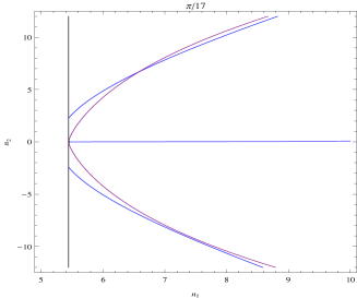
Figure 12: Solutions of the real part (purple) and imaginary part (blue) of the light-cone equation (82) for $A^{\mu}_{\parallel}$ at $\theta=\frac{\pi}{17}$ in the presence of $B$. The black vertical line on the left corresponds to $n_{1}=\frac{1}{s_{\theta}}$

This suggests that below $\theta_{min}$, the system goes to a large index with a large absorption. This type of solution is incompatible with the approximations that we have made to find them $|n_{2}|\ll n_{1}$ etc, such that drawing a definitive conclusion requires using more elaborate numerical methods. This will be the subject of a forthcoming work. Let us only mention here in addition that such solutions with large index/absorption may coexist, above $\theta_{min}$, with the quasi-real solutions that we have exhibited in this work.

Whether or not total reflection occurs inside graphene at low incidences can only be settled with this more complete study. Notice that, if such a phenomenon occurs, it is at small angle of incidence, again at the opposite of what one is accustomed to with geometrical optics.

A brutal transition like this one may also be the sign of a phase transition at the level of fermions or photons. It has often been evoked that chiral symmetry may get broken inside graphene in the presence of a magnetic field (see for example [17]), and that the photon eventually gets an effective mass (breaking of gauge invariance) should also not be systematically rejected before careful investigations have been done.

7.3 A bridge between Quantum Field Theory, quantum optics and nanophysics

Along this limited study, we have pointed at other potentially interesting phenomena that deserve more detailed investigations: a brutal transition below $\theta=\theta_{min}$ in the presence of $B$, the eventual existence, in the same conditions, of several types of solutions (including some with large $n_{1}$ and $n_{2}$), the presence of a “limiting $B=B^{m}$” above which new quantum effects are expected, and, even in the absence of $B$, some intriguing behavior of the refractive index above $\theta=\theta_{max}$ for $\alpha>1$.

The issue whether graphene can be safely described in perturbation theory despite a large electromagnetic coupling deserves also, of course, deeper investigations.

The wavelengths of visible light are $\sim 1000$ times larger than the thickness of graphene. The laws of refraction are therefore not expected to be true. This is confirmed by the existence of solutions to the light-cone equations only satisfying the condition $n\sin\theta>1$, $n$ being the index inside graphene. Since $\theta$ has also been defined as the angle of incidence inside the medium, it is manifestly impossible to satisfy the laws of refraction at its interface with vacuum, which would write $n\sin\theta=1\times\sin\theta_{vacuum}$: the l.h.s. is indeed $>1$ while the r.h.s. is $\leq 1$.

Graphene in external magnetic field is thus certainly not the realm of geometrical optics, but it could well prove, inversely, a privileged test-ground for the interplay between Quantum Field Theory, quantum optics and nanophysics.

Acknowledgments: it is a pleasure to thank M. Vysotsky for his continuous interest and encouragements.

References

- [1] B. MACHET & M.I. VYSOTSKY: “ Modification of Coulomb law and energy levels of the hydrogen atoms in a superstrong magnetic field”, Phys. Rev. D 83 (2011) 025022.
- [2] S.I. GODUNOV, B. MACHET & M.I. VYSOTSKY: “Critical nucleus charge in a superstrong magnetic field: Effects of screening”, Phys. Rev. D 85 (2012) 044058.
- [3] M.O. GOERBIG: “Electronic properties of graphene in a strong magnetic field”, Rev. Mod. Phys. 83 (2011) 1193, and references therein.
- [4] A.H. CASTRO NETO, F. GUINEA, N.M.R. PEREZ, K.S. NOVOSELOV & A.K. GEIM: “The electronic properties of graphene”, Rev. Mod. Phys. 81 (2009) 109.
- [5] J. SCHWINGER: “On Gauge Invariance and Vacuum Polarization”, Phys. Rev. 82 (1951) 664.
- [6] W. DITTRICH & M. REUTER: “Effective Lagrangian in Quantum Electrodynamics”, Lecture Notes in Physics 220 (Springer-Verlag, Berlin Heidelberg 1985).
- [7] WU-YANG TSAI & T. ERBER: “ Photon pair creation in intense magnetic fields”, Phys. Rev. D 10 (1974) 492.
- [8] W. DITTRICH & H. GIES: “Vacuum Birefringence in Strong Magnetic Fields”, hep-ph/9806417, Sandansky 1998, Frontier tests of QED and physics of the vacuum, 29-43.
- [9] N.M.R. PEREZ, A.H. CASTRO NETO & F. GUINEA : “ Dirac fermion confinement in graphene”, Phys. Rev. B 73 (2006) 241403(R).
- [10] S. GODUNOV: “Two-Loop Corrections to the Potential of a Pointlike Charge in a Superstrong Magnetic Field”, Yad. Fiz. 76 (2013) 955 [Phys. Atom. Nucl. 76 (2013) 901].
- [11] R.R. NAIR, P. BLAKE, A.N. GRIGORENKO, K.S. NOVOSELOV, T.J. BOOT, T. STAUBER, N.M.R. PEREZ & A.K. GEIM: “Fine Structure Constant Defines Visual Transparency of Graphene”, Science, vol. 320 (2008) 1308, and references therein.
- [12] WU-YANG TSAI: “Vacuum polarization in homogeneous magnetic fields”, Phys. Rev. D 10 (1974) 2699.
- [13] M.E. PESKIN & D.V. SCHROEDER: “An Introduction to Quantum Field Theory”, Perseus Books (Reading, Massachusetts) 1995.
- [14] Y.W. SOKHOTSKI: “On definite integrals and functions used in series expansions” St. Petersburg, 1873. J. PLEMELJ: “Problems in the sense of Riemann and Klein”, Interscience Publishers, New York, 1964.
- [15] A.V. KOTIKOV & S. TEBER: “Two-loop fermion self-energy in reduced quantum electrodynamics and application to the ultra-relativistic limit of graphene”, arXiv:1312.2430 [hep-ph], Phys. Rev. D89, 065038 (2014).
- [16] J. HOFMANN, E. BARNES & D. SARMA: “Why does graphene behaves as a weakly coupled system ? ”, arXiv:1405.7036 [cond-mat.mes-hall]
- [17] V.P. GUSYNIN, V.A. MIRANSKY & I.A. SHOVKOVY: “Dimensional reduction and catalysis of dynamical symmetry breaking by a magnetic field”, Nucl. Phys. B 462 (1996) 249-290.