High-precision nonadiabatic calculations of dynamic polarizabilities and hyperpolarizabilities for the lowlying vibrational-rotational states of hydrogen molecular ions

Abstract

The static and dynamic electric multipolar polarizabilities and second hyperpolarizabilities of the H${}_{2}^{+}$, D${}_{2}^{+}$, and HD⁺ molecular ions in the ground and first excited states are calculated nonrelativistically using explicitly correlated Hylleraas basis sets. The calculations are fully nonadiabatic; the Born-Oppenheimer approximation is not used. Comparisons are made with published theoretical and experimental results, where available. In our approach, no derivatives of energy functions nor derivatives of response functions are needed. In particular, we make contact with earlier calculations in the Born-Oppenheimer calculation where polarizabilities were decomposed into electronic, vibrational, and rotational contributions and where hyperpolarizabilities were determined from derivatives of energy functions. We find that the static hyperpolarizability for the ground state of HD⁺ is seven orders of magnitude larger than the corresponding dipole polarizability. For the dipole polarizability of HD⁺ in the first excited-state the high precision of the present method facilitates treatment of a near cancellation between two terms. For applications to laser spectroscopy of trapped ions we find tune-out and magic wavelengths for the HD⁺ ion in a laser field. In addition, we also calculate the first few leading terms for long-range interactions of a hydrogen molecular ion and a ground-state H, He, or Li atom.

I Introduction

Polarizabilities and hyperpolarizabilities of molecules can describe linear and nonlinear optical phenomena, such as light scattering from gases and solids and the Kerr effect, and dynamic (or frequency-dependent) values are helpful in designing optical materials and in gauging electric field responses for experiments. While calculations are challenging, there are numerous calculated results for many molecules—static and dynamic polarizabilities and hyperpolarizabilities are available properties in many mature quantum chemistry programs—yet actual fully nonadiabatic ab initio results (obtained without use of the Born-Oppenheimer picture) are rare. In previous studies, it was demonstrated Yan et al. (2003); Zhang and Yan (2004); Bhatia and Drachman (1999, 2000) that a theory based on the explicitly correlated Hylleraas basis set expansion yielded high accuracy nonadiabatic properties of three-body systems. In this paper, we extend the formalism contiguously to multipolar dynamic electric polarizabilities and dynamic second hyperpolarizabilities of the hydrogen molecular ion and its deuterium containing isotopologues in the ground and first excited states. While the formalism presented here is purely nonrelativisitic, the nonadiabatic theory on which it is based is well-tested beyond order $\alpha^{2}~{}\textrm{Ry}$ as progress in calculations of energies of $\textrm{HD}^{+}$, for example, are now at the level where the uncertainties in transition frequencies are of the order of 70 kHz, with unknown effects contributing at order $\alpha^{5}~{}\textrm{Ry}$ Zhong et al. (2012), while refinement of nonadiabatic calculations on simple molecules continues using different approaches Olivares Pilón and Baye (2013); Stanke and Adamowicz (2013); Korobov and Zhong (2012); Kedziera et al. (2006). A comparison of nonrelativistic results for energies is given in Sec. III.

The present calculations, we believe, are of great value for several potential applications. While our approach intrinsically includes rotational and vibrational degrees of freedom it dispenses with the Born-Oppenheimer approximation. Use of the Born-Oppenheimer approximation facilitates the breakdown of polarizabilities and hyperpolarizabilities into “electronic”, “vibrational”, and “rotational” components and the theoretical underpinnings of this picture are well-established, but there are different formulations and subtleties in executing such calculations Bishop et al. (1980); Pandey and Santry (1980); Adamowicz and Bartlett (1986); Bishop (1990); Bishop and Kirtman (1992); Shelton and Rice (1994); Bishop (1998). We show how our results provide insight into these descriptions, allowing direct comparisons with earlier Born-Oppenheimer results, and in Sec. III we use these insights, for example, to resolve a discrepancy found by Olivares Pilón and Baye Olivares Pilón and Baye (2012) in comparing nonadiabatic and Born-Oppenheimer calculations of the dynamic electric quadrupole polarizability. Our method avoids the cumbersome Born-Oppenheimer separation, our tabulated nonadiabatic data can be valuable for estimations or extrapolations of “electronic”, “vibrational”, and “rotational” contributions, when combined with available Born-Oppenheimer calculations Shelton and Rice (1994); Koelemeij (2011). In addition, our nonadiabatic approach does not require derivatives of an energy function Pandey and Santry (1980); Cafiero et al. (2003) nor derivatives of response functions Ingamells et al. (1998), which can introduce additional numerical loss of precision, but it does provide definitive convergence-based error bars thereby allowing us to gauge the accuracy of previous results for hyperpolarizabilities calculated using gradients of fields.

There is much recent interest in trapping molecular ions for precision measurements (of time Schiller et al. (2014a) and of mass Karr et al. (2011), for example) and for realizing quantum computing Shi et al. (2013)—in these cases the responses of ions to applied fields are important considerations Bakalov and Schiller (2012) and our calculations can serve as useful models or references for future studies. We find, for example, that the hyperpolarizabilities of H${}_{2}^{+}$ and D${}_{2}^{+}$ are much larger than the dipole polarizabilities by four orders of magnitude, which confirms Bishop and Solunac (1985) that the Stark shift of H${}_{2}^{+}$ immersed at high field strength would be influenced by the hyperpolarizability. For the ground state of HD⁺, the sign of static dipole polarizability and hyperpolarizability are opposite, suggesting that the hyperpolarizability should be considered in experimental analyses, since the Stark shifts for this system would tend to cancel each other. In Sec. III we present highly accurate calculations of Stark shifts, tune out and magic wavelengths, and nonlinear dynamic hyperpolarizabilities for $\textrm{HD}^{+}$ in the ground and excited states. Finally, the multipolar polarizabilities that we compute enter as parameters in the long-range “polarization potential” Sturrus et al. (1991); Jacobson et al. (1997, 2000), which are effective potential expansions, for the interactions of an electron with the the molecular ion isotopologues. We also calculate the long-range dispersion interactions between H, He, or Li and each of the $\textrm{H}_{2}^{+}$ isotopologues in their ground or first excited states.

In this work, the 2006 CODATA masses Mohr et al. (2008) of the proton and the deuteron are adopted footnote, where

$$m_{p} = 1836.15267247(80)m_{e},$$ (1)

$$m_{d} = 3670.4829654(16)m_{e},$$ (2)

and $m_{e}$ is the electron mass, and atomic units are used throughout unless specifically mentioned. The polarizabilities and hyperpolarizabilities are presented in atomic units Shelton and Rice (1994); conversion factors to SI units are given in, for example, the reviews by Bishop Bishop (1990) and by Shelton and Rice Shelton and Rice (1994). In this nonrelativistic study we neglect finite temperature effects Bishop et al. (1988); Shelton and Rice (1994), hyperfine structure Schiller et al. (2014a, b), and we do not consider the first hyperpolarizability (which is only non zero for $\textrm{HD}^{+}$).

II THEORY AND METHOD

II.1 Hamiltonian and Hylleraas basis

In the present work, we treat the hydrogen molecular ion as a three-body Coulombic system; the calculations are fully nonadiabatic (the Born-Oppenheimer approximation is not used). Taking one of the nuclei as particle 0, the electron is chosen as particle 1 and the other nucleus is seen as particle 2. In the center of mass frame, the Hamiltonian can be written as

$$H_{0} = -\sum_{i=1}^{2}\frac{1}{2\mu_{i}}\nabla_{i}^{2}-\frac{1}{m_{0}}\sum_{i>j\geq 1}^{2}\nabla_{i}\cdot\nabla_{j}+q_{0}\sum_{i=1}^{2}\frac{q_{i}}{r_{i}}+\sum_{i>j\geq 1}^{2}\frac{q_{i}q_{j}}{r_{ij}}\,,$$ (3)

where $\mu_{i}=m_{i}m_{0}/(m_{i}+m_{0})$ is the reduced mass between particle $i$ and particle $0$, $q_{i}$ is the charge of the $i$th particle, $\mathbf{r}_{i}$ is the position vector between particle $i$ and particle $0$, and $r_{ij}=|{\bf{r}}_{i}-{\bf{r}}_{j}|$ is the inter-particle separation.

The wave functions are constructed in terms of the explicitly correlated Hylleraas coordinates as

$$\phi_{ijk}({\bf{r}}_{1},{\bf{r}}_{2})=r_{1}^{i}r_{2}^{j}r_{12}^{k}e^{-\alpha r_{1}-\beta r_{2}}\mathcal{Y}_{\ell_{1}\ell_{2}}^{LM}(\hat{{\bf{r}}}_{1},\hat{{\bf{r}}}_{2}),$$ (4)

where $r_{2}^{j}e^{-\beta r_{2}}$ sufficiently represents the vibrational modes between the nuclei if $j$ and $\beta$ are chosen big enough Yan et al. (2003), $\mathcal{Y}_{\ell_{1}\ell_{2}}^{LM}(\hat{{\bf{r}}}_{1},\hat{{\bf{r}}}_{2})$ is a vector-coupled product of spherical harmonics,

$$\mathcal{Y}_{\ell_{1}\ell_{2}}^{LM}(\hat{{\bf{r}}}_{1},\hat{{\bf{r}}}_{2})=\sum_{m_{1},m_{2}}\langle\ell_{1}m_{1};\ell_{2}m_{2}|LM\rangle Y_{\ell_{1}m_{1}}(\hat{{\bf{r}}}_{1})Y_{\ell_{2}m_{2}}(\hat{{\bf{r}}}_{2})\,,$$ (5)

and the nonlinear parameters $\alpha$ and $\beta$ are optimized using Newton’s method. All terms in Eq.(4) are included such that

$$i+j+k\leq\Omega\,,$$ (6)

where $\Omega$ is an integer, and the convergence for the energy eigenvalue is studied as $\Omega$ is increased progressively. The computational details used in evaluating the necessary matrix elements of the Hamiltonian are given in Ref. Yan and Drake (1996).

II.2 Polarizability and Hyperpolarizability

When the hydrogen molecular ion is exposed to a weak external electric field ${\cal{E}}$, the second-order Stark shift for the rovibronic state is

$$\Delta E_{2}=-\frac{{\cal{E}}^{2}}{2}[\alpha_{1}(\omega)+\alpha_{1}^{(T)}(\omega)g_{2}(L,M)]\,,$$ (7)

where $L$ is the angular momentum with magnetic quantum number $M$, $g_{2}(L,M)$ is the only $M$-dependent part,

$$g_{2}(L,M) = \frac{3M^{2}-L(L+1)}{L(2L-1)},\ \ L\geq 1\,,$$ (8)

and $\omega$ is the frequency of the external electric field in the $z$-direction. The dynamic scalar and tensor dipole polarizabilities, respectively, are $\alpha_{1}(\omega)$ and $\alpha_{1}^{(T)}(\omega)$; when $\omega=0$, they are called, respectively, the static scalar and tensor dipole polarizabilities. The derivation of the expressions for the dynamic polarizabilities $\alpha_{1}(\omega)$ and $\alpha_{1}^{(T)}(\omega)$ are similar to those described in Ref. Tang et al. (2010). In particular, for the case of rovibronic ground-state with $L=0$,

$$\alpha_{1}(\omega)=\alpha_{1}(P,\omega)\,,\qquad\alpha_{1}^{(T)}(\omega)=0,$$ (9)

with $\alpha_{1}(L_{a},\omega)$ following the general expression of $2^{\ell}$-pole partial dynamic polarizabilities,

$$\alpha_{\ell}(L_{a},\omega) = \frac{8\pi}{(2\ell+1)^{2}(2L+1)}\sum_{n}\frac{\Delta E_{n0}|\langle n_{0}L\|T_{\ell}\|nL_{a}\rangle|^{2}}{\Delta E_{n0}^{2}-\omega^{2}}\,,$$ (10)

where $n_{0}$ and $n$, respectively, label the initial state and the intermediate state and $\Delta E_{n0}=E_{n}-E_{n_{0}}$ is the difference between the initial and intermediate state energies. The detailed formula for the $2^{\ell}$-pole transition operator $T_{\ell}$ in the center of mass frame is given in Ref. Tang et al. (2009a).

For the rovibronic excited-state with $L=1$, $\alpha_{1}(\omega)$ and $\alpha_{1}^{(T)}(\omega)$ can be written

$$\alpha_{1}(\omega) = \alpha_{1}(S,\omega)+\alpha_{1}(P,\omega)+\alpha_{1}(D,\omega)\,,$$ (11)

$$\alpha_{1}^{(T)}(\omega) = -\alpha_{1}(S,\omega)+\frac{1}{2}\alpha_{1}(P,\omega)-\frac{1}{10}\alpha_{1}(D,\omega)\,,$$ (12)

where $\alpha_{1}(P,\omega)$ denotes the contribution of nucleus 2 and electron 1 both being in $p$ configuration to form a total angular momentum of $P$. The expressions for other multipole dynamic polarizabilities are derived similarly to those for the dipole polarizabilities Tang et al. (2009a, b, 2010).

The fourth-order Stark shift for the rovibronic state can be written in the form,

$$\Delta E_{4} = -\frac{{\cal{E}}^{4}}{24}\bigg{[}\gamma_{0}(-\omega_{\sigma};\omega_{1},\omega_{2},\omega_{3})+\gamma_{2}(-\omega_{\sigma};\omega_{1},\omega_{2},\omega_{3})\,g_{2}(L,M)+\gamma_{4}(-\omega_{\sigma};\omega_{1},\omega_{2},\omega_{3})\,g_{4}(L,M)\bigg{]}\,,$$

where $g_{4}(L,M)$ is only dependent on the angular momentum quantum number $L$ and magnetic quantum number $M$,

$$g_{4}(L,M)=\frac{3(5M^{2}-L^{2}-2L)(5M^{2}+1-L^{2})-10M^{2}(4M^{2}-1)}{L(2L-1)(2L-2)(2L-3)},\,L\geq 2,$$ (14)

and $\omega_{i}$ are the frequencies of the external electric field in the three directions with $\omega_{\sigma}=\omega_{1}+\omega_{2}+\omega_{3}$. The dynamic scalar second hyperpolarizability is $\gamma_{0}(-\omega_{\sigma};\omega_{1},\omega_{2},\omega_{3})$, and the dynamic tensor second hyperpolarizabilities are $\gamma_{2}(-\omega_{\sigma};\omega_{1},\omega_{2},\omega_{3})$ and $\gamma_{4}(-\omega_{\sigma};\omega_{1},\omega_{2},\omega_{3})$. (From this point on, we will omit “second” when referring to the hyperpolarizabilities.) When all $\omega_{i}=0$, the functions are called static hyperpolarizabilities. In particular, for the rovibronic excited-state with $L=0$ only the dynamic scalar hyperpolarizability remains and it is

$$\gamma_{0}(-\omega_{\sigma};\omega_{1},\omega_{2},\omega_{3})=\frac{16\pi^{2}}{9}\big{[}\frac{1}{9}\mathcal{T}(1,0,1;\omega_{1},\omega_{2},\omega_{3})+\frac{2}{45}\mathcal{T}(1,2,1;\omega_{1},\omega_{2},\omega_{3})\big{]},$$ (15)

where

$$\mathcal{T}(L_{a},L_{b},L_{c};\omega_{1},\omega_{2},\omega_{3}) = \sum_{P}\bigg{[}\sum_{kmn}\frac{\langle n_{0}L\|T_{1}^{\mu_{1}}\|mL_{a}\rangle\langle mL_{a}\|T_{1}^{\mu_{2}}\|nL_{b}\rangle\langle nL_{b}\|T_{1}^{\mu_{3}}\|kL_{c}\rangle\langle kL_{c}\|T_{1}^{\mu_{4}}\|n_{0}L\rangle}{(\Delta E_{mn_{0}}-\omega_{\sigma})(\Delta E_{nn_{0}}-\omega_{1}-\omega_{2})(\Delta E_{kn_{0}}-\omega_{1})}$$ (16)

$$- \delta(L_{b},L)\sum_{m}\frac{\langle n_{0}L\|T_{1}^{\mu_{1}}\|mL_{a}\rangle\langle mL_{a}\|T_{1}^{\mu_{2}}\|n_{0}L\rangle}{(\Delta E_{mn_{0}}-\omega_{\sigma})}$$

$$\times \sum_{k}\frac{\langle n_{0}L\|T_{1}^{\mu_{3}}\|kL_{c}\rangle\langle kL_{c}\|T_{1}^{\mu_{4}}\|n_{0}L\rangle}{(\Delta E_{kn_{0}}+\omega_{2})(\Delta E_{kn_{0}}-\omega_{1})}\bigg{]},$$

the $\sum_{P}$ implies a summation over the 24 terms generated by permuting the pairs ($-\omega_{\sigma}/T_{1}^{\mu_{1}}$), ($\omega_{1}/T_{1}^{\mu_{2}}$), ($\omega_{2}/T_{1}^{\mu_{3}}$), and ($\omega_{3}/T_{1}^{\mu_{4}}$), where the superscripts $\mu_{i}$ are introduced for the purpose of labeling the permutations Pipin and Bishop (1992).

III Results And Discussion

III.1 Energies

Table 1: Energies (in a.u.) for the H${}_{2}^{+}$, D${}_{2}^{+}$, and HD⁺ ions for $\upsilon\leq 3$ and $L\leq 3$. For each value of $(\upsilon,L)$ in the first column, the first row gives the present result resulting from a single diagonalization of the lowest $\upsilon$ state for a given $L$. Where a value of $(\upsilon,L)$ has a second row (H${}_{2}^{+}$ and HD⁺) the entry on the second row lists the result of Korobov Korobov (2006), for which each value is the result of a separate minimization (see text for further discussion). The number in parentheses represents the computational uncertainty in the last digit.

($\upsilon,L$)	H${}_{2}^{+}$	D${}_{2}^{+}$	HD+
(0,0)	$-$0.597 139 063 079 392 297 758(4)	$-$0.598 788 784 304 562 857 67(6)	$-$0.597 897 968 608 954 700 9(1)
	$-$0.597 139 063 079 39		$-$0.597 897 968 609 03
(1,0)	$-$0.587 155 679 164 695 13(2)	$-$0.591 603 121 831 520 71(3)	$-$0.589 181 829 556 745 7(1)
	$-$0.587 155 679 096 19		$-$0.589 181 829 556 96
(2,0)	$-$0.577 751 904 547 41(7)	$-$0.584 712 206 896 55(1)	$-$0.580 903 700 218(1)
	$-$0.577 751 904 415 08		$-$0.580 903 700 218 37
(3,0)	$-$0.568 908 498 91(7)	$-$0.578 108 591 285 37(2)	$-$0.573 050 546(1)
	$-$0.568 908 498 730 86		$-$0.573 050 546 551 87
(0,1)	$-$0.596 873 738 784 713 077 8(1)	$-$0.598 654 873 192 605 311 3(3)	$-$0.597 698 128 192 126 71(1)
	$-$0.596 873 738 784 71		$-$0.597 698 128 192 21
(1,1)	$-$0.586 904 320 919 191 59(5)	$-$0.591 474 211 455 255 47(6)	$-$0.588 991 111 991 818(4)
	$-$0.586 904 320 919 19		$-$0.588 991 111 992 04
(2,1)	$-$0.577 514 034 057 4(2)	$-$0.584 588 169 503 82(3)	$-$0.580 721 828 12(1)
	$-$0.577 514 034 057 45		$-$0.580 721 828 120 93
(3,1)	$-$0.568 683 708 2(2)	$-$0.577 989 311 81(2)	$-$0.572 877 277(3)
	$-$0.568 683 708 260 19		$-$0.572 877 277 094 21
(0,2)	$-$0.596 345 205 489 114 7(2)	$-$0.598 387 585 778 605 864(3)	$-$0.597 299 643 351 683 2(1)
	$-$0.596 345 205 489 39		$-$0.597 299 643 351 78
(1,2)	$-$0.586 403 631 528 0(8)	$-$0.591 216 909 547 769 2(4)	$-$0.588 610 829 389 5(2)
	$-$0.586 403 631 528 69		$-$0.588 610 829 389 79
(2,2)	$-$0.577 040 237 1(6)	$-$0.584 340 598 262 86(3)	$-$0.580 359 195 2(6)
	$-$0.577 040 237 163 02		$-$0.580 359 195 199 88
(3,2)	$-$0.568 235 98(5)	$-$0.577 751 241 74(1)	$-$0.572 531 8(2)
	$-$0.568 235 992 971 58		$-$0.572 531 810 325 97
(0,3)	$-$0.595 557 638 980 309 2(7)	$-$0.597 987 984 710 141(4)	$-$0.596 704 882 761 75(3)
	$-$0.595 557 638 980 31		$-$0.596 704 882 761 89
(1,3)	$-$0.585 657 611 877(1)	$-$0.590 832 246 988(4)	$-$0.588 043 264 163(2)
	$-$0.585 657 611 877 66		$-$0.588 043 264 162 84
(2,3)	$-$0.576 334 350 2(2)	$-$0.583 970 493 6(1)	$-$0.579 818 002 1(1)
	$-$0.576 334 350 219 63		$-$0.579 818 002 027 87
(3,3)	$-$0.567 569 02(5)	$-$0.577 395 352 1(9)	$-$0.572 016 269 2(4)
	$-$0.567 569 034 833 51		$-$0.572 016 269 232 51

The converged energies of the H${}_{2}^{+}$, D${}_{2}^{+}$, and HD⁺ molecular ions from the present Hylleraas calculations for the rovibronic levels $(\upsilon,L)$ with $\upsilon\leq 3$ and $L\leq 3$ are listed in Table 1 and compared to the calculations of Korobov Korobov (2006) for H${}_{2}^{+}$ and HD⁺, who used a different form of basis sets with pseudorandom complex exponents and the 2002 CODATA values of the proton and deuteron masses Mohr and Taylor (2005). For the $(0,0)$ state of H${}_{2}^{+}$ the present result contains 20 significant figures, which improves by six orders of magnitude the result of Korobov. Other results in Table 1 are converged to at least 10 significant digits. For states $(\upsilon\geq 1,L)$ the energies are less accurate than the corresponding $(0,L)$ states since our calculations in this paper are for applications to “sum over states” determinations of polarizabilities. Thus, the energies in Table 1 for a given system and value of $(\upsilon,L)$ correspond to optimized nonlinear variational parameters for the corresponding $\upsilon=0$ state. In contrast, calculations by Korobov Korobov (2006) optimized the bases for each value $(\upsilon,L)$, and as expected, our present values are systematically more positive compared to his. Recently, even more accurate energy values for $\textrm{HD}^{+}$ were published in Ref. Tian et al. (2012) using basis sets similar to the present approach, but with specific optimization and diagonalization for each separate energy level $(\upsilon,L)$. (Accurate treatments of relativistic corrections to the ground and first excited states were presented recently for $\textrm{H}_{2}^{+}$ Korobov (2008); Zhong et al. (2009) and for $\textrm{HD}^{+}$ Korobov (2008); Zhong et al. (2012).)

III.2 Ground-state static polarizabilities and hyperpolarizabilities

Table 2: Convergence of static multipole polarizabilities $\alpha_{1}(0)$, $\alpha_{2}(0)$, and hyperpolarizability $\gamma_{0}(0;0,0,0)$ (in a.u.) for the rovibronic ground-state $(\upsilon=0,L=0)$ of the H${}_{2}^{+}$ ion. $N_{S}$, $N_{P}$, and $N_{D}$, respectively, represent the number of basis sets for the initial-state of $S$ symmetry, intermediate states of $P$ symmetry, and intermediate states of $D$ symmetry. The extrapolated values for each quantity are listed on the last line with the computational uncertainties of the last digits in parentheses.

$\alpha_{1}(0)$		$\alpha_{2}(0)$		$\gamma_{0}(0;0,0,0)$
($N_{S}$,$N_{P}$)	value	($N_{S}$,$N_{D}$)	value	($N_{S}$,$N_{P}$,$N_{D}$)	value
(420,532)	3.168 723 735 424 03	(420,561)	1371.890 552 022 99	(420,532,561)	11479.750 406 991
(680,695)	3.168 725 614 348 09	(680,727)	1371.894 443 542 72	(680,695,727)	11479.793 416 663
(1036,1120)	3.168 725 797 655 76	(1036,954)	1371.894 963 825 42	(1036,1120,954)	11479.795 141 858
(1255,1388)	3.168 725 804 884 54	(1255,1225)	1371.895 138 590 14	(1255,1388,1225)	11479.804 857 235
(1504,1697)	3.168 725 805 220 47	(1504,1544)	1371.895 140 761 38	(1504,1697,1544)	11479.805 065 320
(1785,2050)	3.168 725 805 275 76	(1785,1915)	1371.895 141 217 43	(1785,2050,1915)	11479.805 067 728
(2100,2450)	3.168 725 805 286 34	(2100,2342)	1371.895 141 236 83	(2100,2450,2342)	11479.805 069 686
(2451,2900)	3.168 725 805 288 58	(2451,2829)	1371.895 141 237 55	(2451,2900,2829)	11479.805 069 814
Extrapolated	3.168 725 805 289(1)	Extrapolated	1371.895 141 24(1)	Extrapolated	11479.805 07(1)

Table 2 presents a convergence study of the static multipole polarizabilities $\alpha_{1}(0)$ and $\alpha_{2}(0)$, and the static hyperpolarizability $\gamma_{0}(0;0,0,0)$ for H${}_{2}^{+}$ in the rovibronic ground-state $(\upsilon=0,L=0)$. The number of basis sets for the state of interest is indicated by $N_{S}$, the number used for the intermediate states with $P$ symmetry and $D$ symmetry are indicated by $N_{P}$ and $N_{D}$ respectively. The extrapolated values are obtained by assuming that the ratio between two successive differences stays constant as the number of basis sets used becomes infinitely large. The static polarizabilities $\alpha_{1}(0)$ and $\alpha_{2}(0)$ converged quickly to, respectively, twelve and eleven digits as the dimensions of the basis sets $N_{S}$, $N_{P}$, and $N_{D}$ were increased. The static hyperpolarizability, which is larger than $\alpha_{1}(0)$ by four orders of magnitude, converged to the ninth significant digit. Similar convergence tests for $\alpha_{3}(0)$ and $\alpha_{4}(0)$ of H${}_{2}^{+}$ yield the extrapolated results listed in Table 3.

Table 3: Static polarizabilities and hyperpolarizabilities (in a.u.) of H${}_{2}^{+}$, HD⁺, and D${}_{2}^{+}$ ions in the ground-state $(\upsilon=0,L=0)$. The numbers in parentheses represent the computational uncertainties obtained by extrapolation. The first line gives the present values calculated using the CODATA 2006 masses. The second line gives the present values calculated using $m_{p}=1836.152701$ and $m_{d}=3670.483014$ for comparison with Refs. Yan et al. (2003); Hilico et al. (2001); Olivares Pilón and Baye (2012); Korobov (2001); Bhatia and Drachman (2000); Moss and Valenzano (2002). The numbers in the square brackets for $\gamma_{0}$ denote powers of ten.

	$\alpha_{1}(0)$
Author and Reference	H${}_{2}^{+}$	D${}_{2}^{+}$	HD+
Present	3.168 725 805 289(1)	3.071 988 697 188(1)	395.306 325 6742(2)
Present	3.168 725 802 676(1)	3.071 988 695 66(7)	395.306 328 7970(6)
Yan et al. Yan et al. (2003)	3.168 725 802 67(1)	3.071 988 695 7(1)	395.306 328 7972(1)
Moss and Valenzano Moss and Valenzano (2002)			395.306
Bhatia and Drachman Bhatia and Drachman (2000)			395.289
Hilico et al. Hilico et al. (2001)	3.168 725 803(1)	3.071 988 696(1)
Korobov Korobov (2001)	3.168 725 76	3.071 988 68
Korobov Korobov (2001)	3.168 573 62	3.071 838 77
Jacobson et al. Jacobson et al. (2000)	3.167 96(15)	3.071 87(54)
System (Present result)	$\alpha_{2}(0)$	$\alpha_{3}(0)$	$\alpha_{4}(0)$	$\gamma_{0}(0;0,0,0)$
H${}_{2}^{+}$	1 371.895 141 24(1)	23.975 062 60(4)	571.963 841(2)	1.147 980 507(1)[4]
D${}_{2}^{+}$	2 587.094 024 00(1)	22.890 669 73(1)	819.239 589(4)	1.967 663 142(3)[4]
HD+	2 050.233 354 19(1)	773.42 727 01(1)	1434.30 534(1)	$-$3.356 560 39(2)[9]

The static multiple polarizabilities and hyperpolarizabilities for the ground-state $(\upsilon=0,L=0)$ of H${}_{2}^{+}$, HD⁺, and D${}_{2}^{+}$ are listed in Table 3. The polarizabilities and hyperpolarizabilities for the homonuclear molecular ions H${}_{2}^{+}$ and D${}_{2}^{+}$ have the same magnitudes. For the heteronuclear ion HD⁺ the corresponding values are much larger than those for H${}_{2}^{+}$ and for D${}_{2}^{+}$, due to the much smaller value of the first allowed transition energy. Note that the hyperpolarizability of HD⁺ has opposite sign from H${}_{2}^{+}$ and D${}_{2}^{+}$ due to the sign of the contribution from the two terms of Eq. (15).

Table 3 also gives a comparison with selected previous works for the static dipole polarizabilities in the rovibronic ground-state $(0,0)$ calculated using nonadiabatic methods (some earlier results for $\textrm{H}_{2}^{+}$ can be found in Ref. Taylor et al. (1999)). In order to facilitate comparison of the present dipole polarizabilities with those of Yan et al. Yan et al. (2003), we repeated the calculations by using the same nuclear masses as they used, and the resulting values are listed in the second line. The agreement for $\alpha_{1}(0)$ could hardly have been better. However, the present static dipole polarizability of H${}_{2}^{+}$ is accurate to three parts in $10^{13}$, which improves by one order of magnitude the result of Yan et al. For the static dipole polarizability of H${}_{2}^{+}$, our polarizability of 3.168 725 805 289(1) is 0.025% different from the experimental value of 3.167 96(15) Jacobson et al. (2000). For D${}_{2}^{+}$, our value is in good agreement with the less accurate result of Hilico et al. Hilico et al. (2001) and slightly larger than the result of Yan et al. Yan et al. (2003). The present dipole polarizability 3.071 988 697 188(1) of D${}_{2}^{+}$ agrees with the experimental value 3.07187(54) at the level of 0.004%. For HD⁺, our result is much more accurate than the early result of Moss and Valenzano Moss and Valenzano (2002). Some other nonadiabatic calculations of the quadrupole (and higher order) polarizabilities are given in Refs. Yan et al. (2003); Olivares Pilón and Baye (2012) and we are in good agreement. There is a previous nonadiabatic calculation of the second hyperpolarizability for H${}_{2}^{+}$: Moss and Valenzano Moss and Valenzano (2002) find $\gamma=1.14\times 10^{4}$, in harmony with our result.

It is interesting to examine in more detail the quadrupole polarizibility and second hyperpolarizability calculations with previous Born-Oppenheimer treatments, where the quantities are separated into “electronic”, “vibrational”, and “rotational” contributions Bishop and Lam (1988). As exhibited in Table 3, the relative magnitude of $\alpha_{2}(0)$ is much larger than those of $\alpha_{1}(0)$ and $\alpha_{3}(0)$, which is related to the available low-lying virtual state in the energy denominator (a similar argument pertains to $\alpha_{4}(0)$). In the Born-Oppenheimer approach, the virtual excitation corresponds to no change in the electronic or vibrational quantum number, but a change in the rotational quantum number by 2. Bishop and Lam Bishop and Lam (1988), (see their table 7), found $\alpha_{2}(0)=1370.7$ a.u., composed of electronic, vibrational, and rotational contributions of, respectively, $4.8$ a.u., $3.69$ a.u., and $1362.24$ a.u., where the relatively larger rotational contribution reflects the low-lying virtual excitation. In a recent paper, Olivares Pilón and Baye Olivares Pilón and Baye (2012) compared their total nonadiabatic calculation of $\alpha_{2}(0)$ for the ground state to a second order perturbation theoretic sum over the first four vibrational states (their Eq. (25)) using matrix elements from their nonadiabatic calculation. They found that the nonadiabatic result was greater by an additive factor of $4.793$, compared to the summation and attributed this to “the contribution of the continuum.” In the language of Bishop and Lam Bishop and Lam (1988), the summation corresponds to including most of the “vibrational” and “rotational” components of $\alpha_{2}(0)$. The missing quantity is supplied by Bishop and Lam’s “electronic” component of $4.8$. Evidently, the partial sum of Olivares Pilón and Baye does not converge to the correct value simply because of the neglect of higher electronic excitations.

The magnitude of the static hyperpolarizability can also be understood along similar lines in Born-Oppenheimer picture. Earlier work using finite field methods by Bishop and Solunac Bishop and Solunac (1985) and by Adamowicz and Bartlett Adamowicz and Bartlett (1986) established that nonadiabatic effects were not the source of the large hyperpolarizability. Subsequently, Bishop and Lam Bishop and Lam (1988) calculated $\gamma(0)=11537.16$, with electronic, vibrational, and rotational contributions of, respectively, $29.76$, $568.7$, and $10945.13$, where again the larger rotational contribution is mainly due to the virtual transition where the rotational quantum number changes by 2.

Dynamic hyperpolarizabilities pertain to the four nonlinear optical processes (cf. Refs. Orr and Ward (1971); Pipin and Bishop (1992); Shelton and Rice (1994)): Thus, the quantity $\gamma_{0}(-\omega;\omega,0,0)$ is the dc Kerr effect, $\gamma_{0}(-\omega;\omega,\omega,-\omega)$ represents degenerate four-wave mixing (DFWM), $\gamma_{0}(-2\omega;0,\omega,\omega)$ is electric-field-induced second-harmonic generation (ESHG) and $\gamma_{0}(-3\omega;\omega,\omega,\omega)$ is third-harmonic generation (THG).

In the Born-Oppenheimer approach, the rotational contributions to the dynamic hyperpolarizabilities for the dc Kerr and DFWM processes at optical wavelengths are expected to be comparable to $\gamma(0)$ while the rotational contributions to the ESHG and THG processes are expected to be much reduced in comparison to $\gamma(0)$ Shelton and Rice (1994). For $\textrm{H}_{2}^{+}$, we calculated the dc Kerr, DFWM, and ESHG hyperpolarizabilities at a wavelength of 632.8 nm. Using the available Born-Oppenheimer calculations of the electronic contributions from Bishop and Lam Bishop and Lam (1987) (their tables 2–4) (at the $\textrm{H}_{2}^{+}$ equilibrium internuclear distance 2 a.u.) and the vibrational contributions (their table 7), we estimated the rotational contributions by subtraction from our nonadiabatic values. The results are given in Table 4. The nonadiabatic calculations were carried out using the methods described herein with the largest basis set $(N_{s},N_{p},N_{d})=(2840,2900,2829)$ and were converged values. (Unfortunately, we were unable to obtain a converged value for THG at this wavelength.) Nevertheless, the results yield estimates of the rotational components of dc Kerr and DFWM that are comparable to the static value. For example, at 632.8 nm (He-Ne laser), we find that the dc Kerr rotational contribution is around $3787$ compared to the ESHF rotational contribution of $-35$.

Table 4: For $\mbox{H}_{2}^{+}$, estimation of rotational contributions to the dc Kerr, DFWM, and ESHG processes, in the Born-Oppenheimer picture, using tabulated electronic and vibrational values and the present nonadiabatic values, at wavelength of 632.8 nm. The values for the “Electronic” component” correspond to the internuclear distance of 2 a.u.

component	dc Kerr	DFWM	ESHG
Nonadiabatic (total)	4028.6	8445.1	14.631
Electronic (Ref. Bishop and Lam (1987))	54.3	56.2	58.3
Vibrational (Ref. Bishop and Lam (1987))	187.21	388.87	-8.65
Rotational (row 1-(row 2+row3))	3787	8000	-35.0

III.3 Dynamic dipole polarizabilities and hyperpolarizabilities for the rovibronic ground-state of HD⁺

Table 5: Dynamic dipole polarizabilities and hyperpolarizabilities (in a.u.) for HD⁺ in the ground-state $(\upsilon=0,L=0)$ for photon energies $\omega\leq 0.0004$ a.u. The numbers in parentheses represents the computational uncertainties. The numbers in the square brackets denote powers of ten.

$\omega\times 10^{4}$	$\alpha_{1}(\omega)$	dc Kerr	DFWM	ESHG	THG
0.2	399.273 277 88(1)	$-$3.41610834(1)[9]	$-$3.47659308(2)[9]	$-$3.54049773(2)[9]	$-$3.74430183(2)[9]
0.4	411.670 828 83(1)	$-$3.60545269(2)[9]	$-$3.87061373(2)[9]	$-$4.20449102(2)[9]	$-$5.57473833(2)[9]
0.6	434.153 094 36(1)	$-$3.96135711(2)[9]	$-$4.66118020(2)[9]	$-$5.89905124(3)[9]	$-$2.04245391(1)[10]
0.8	470.133 273 96(1)	$-$4.56456592(2)[9]	$-$6.14508585(2)[9]	$-$1.159595160(4)[10]	9.78040986(3)[9]
1.0	526.283 388 35(1)	$-$5.58859503(3)[9]	$-$9.05764398(4)[9]	2.99296605(1)[12]	4.05178750(1)[9]
1.2	616.411 116 77(1)	$-$7.44289693(3)[9]	$-$1.549390983(5)[10]	1.310381956(4)[10]	2.816792369(6)[9]
1.4	773.207 487 30(1)	$-$1.128714230(5)[10]	$-$3.304470220(9)[10]	7.89267238(2)[9]	2.506628276(6)[9]
1.6	1095.46 735 839(1)	$-$2.165280366(8)[10]	$-$1.033521867(2)[11]	7.29733829(2)[9]	2.799248441(7)[9]
1.8	2081.02 392 881(1)	$-$7.39271980(2)[10]	$-$7.964170683(8)[11]	1.042204934(1)[10]	4.53270763(2)[9]
2.0	$-$245402.484 3(1)	$-$9.60586446(3)[14]	1.51083701452(7)[18]	$-$1.016296893(1)[12]	$-$4.88278453(2)[11]
2.2	$-$1846.878 075 95(3)	$-$5.00377102(2)[10]	7.760677632(7)[11]	$-$6.877974834(7)[9]	$-$3.60827031(3)[9]
2.4	$-$883.279 541 49(2)	$-$1.030699336(3)[10]	1.090946710(2)[11]	$-$3.253912120(4)[9]	$-$1.85432993(3)[9]
2.6	$-$562.828 160 15(2)	$-$3.659961421(7)[9]	4.08371648(1)[10]	$-$2.367173671(6)[9]	$-$1.46202643(3)[9]
2.8	$-$403.893 734 87(1)	$-$1.577815323(2)[9]	2.94181712(1)[10]	$-$2.67134745(1)[9]	$-$1.78534388(5)[9]
3.0	$-$309.565 802 26(1)	$-$7.219101053(4)[8]	$-$2.874893746(7)[11]	3.66561097(3)[10]	2.6441199(1)[10]
3.2	$-$247.474 914(1)	$-$3.120300419(3)[8]	$-$5.555601770(5)[9]	9.3765350(2)[8]	7.2597679(4)[8]
3.4	$-$203.741 252(1)	$-$9.55821852(5)[7]	$-$1.473800328(4)[9]	3.20406687(8)[8]	2.6341471(2)[8]
3.6	$-$171.427 953(1)	2.69257734(6)[7]	$-$5.41613704(5)[8]	1.51419712(6)[8]	1.2971185(1)[8]
3.8	$-$146.685 806(1)	1.00270127(1)[8]	$-$2.30385033(5)[8]	8.4768476(4)[7]	7.3438222(8)[7]
4.0	$-$127.209 551(1)	1.46714081(1)[8]	$-$1.05875887(4)[8]	5.3872799(4)[7]	4.5225693(6)[7]

Since the transition $(0,0)\rightarrow(0,1)$ is a forbidden transition for the H${}_{2}^{+}$ and D${}_{2}^{+}$ ions, the first allowed transitions are at about $\omega=0.1903$ a.u. for H${}_{2}^{+}$ and $\omega=0.2004$ a.u. for D${}_{2}^{+}$, corresponding to “electronic transitions” (in the Born-Oppenheimer picture) and which are not in the visible spectrum. Thus, in this subsection we concentrate only on the dynamic dipole polarizability and hyperpolarizability of the HD⁺ system, for which optical transitions can occur. Table 5 presents selectively some values of dynamic dipole polarizabilities and hyperpolarizabilities for ground-state HD⁺. All of the values are accurate to at least nine significant figures. The effect of the $(0,0)$ to $(0,1)$ resonance near the energy $2.0\times 10^{-4}$, see Table 1, on the quantities tabulated is apparent.

Figs. 1–3 show the dynamic dipole polarizability $\alpha_{1}(\omega)$ of HD⁺ in the ground state as a function of wavelength $\lambda=c/\omega$ in $\mu\textrm{m}$. The perpendicular lines represent the positions of resonant transitions. That there are many resonance transitions as $\lambda\rightarrow 0$ $\mu\textrm{m}$ is evident in Fig 1. However, for the wavelengths $\lambda=4-10$ $\mu\textrm{m}$, shown in Fig. 2, and the wavelengths $\lambda=10-300$ $\mu\textrm{m}$, shown in Fig. 3, there is only one transition in each range. In the inserts for Figs. 2 and 3 the plots are magnified to show the positions where $\alpha_{1}(\omega)=0$. In Fig. 2, the transition $(0,0)\rightarrow(1,1)$ occurs at $\lambda=5.115454421$ $\mu\textrm{m}$ (or photon energy of 0.008907 a.u.) and $\alpha_{1}(\omega)=0$ at $\lambda=5.05024967$ $\mu\textrm{m}$ (0.009022 a.u.). In Fig. 3, the transition $(0,0)\rightarrow(0,1)$ occurs at $\lambda=227.816763$ $\mu\textrm{m}$ and $\alpha_{1}(\omega)=0$ occurs at $\lambda=20.5147918$ $\mu\textrm{m}$. Our results for the $(0,0)$ state are in good agreement with the less accurate results of Koelemeij Koelemeij (2011), who combined the nonadiabatic polarizability calculations of Moss and Valenzano Moss and Valenzano (2002) with vibrational-rotational energies and electric dipole matrix elements calculated in the Born-Oppenheimer picture to obtain values of $\alpha_{1}(\omega)$ in the infrared. In Fig. 4 the various hyperpolarizabilities (dc Kerr, DFWM, ESHG, and THG) are plotted over the energy range $0<\omega<4\times 10^{-4}$ a.u. The first resonant transition is prominent near $2.0\times 10^{-4}$ a.u. Note that sign changes for ESHF and THG occur at lower energies and sign changes for DFWM, ESHG, and THG occur at higher energies as well, due to the complicated perturbation theoretic expressions.

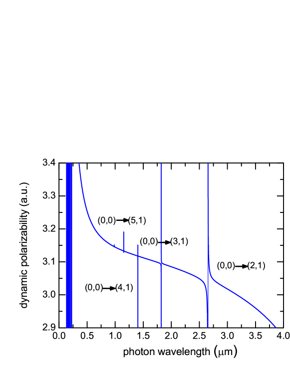
Figure 1: (Color online) Dynamic dipole polarizability $\alpha_{1}(\omega)$ (in a.u.) for the rovibronic ground-state $(\upsilon=0,L=0)$ of the HD⁺ ion for photon wavelengths from 0 to 4 $\mu\textrm{m}$. The resonances $(0,0)\rightarrow(\upsilon,1)$ in the dynamic polarizability are marked.

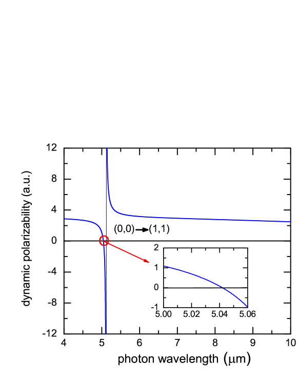
Figure 2: (Color online) Dynamic dipole polarizability $\alpha_{1}(\omega)$ (in a.u.) for the rovibronic ground-state $(\upsilon=0,L=0)$ of the HD⁺ ion for photon wavelengths from 4 to 10 $\mu\textrm{m}$. The resonance $(0,0)\rightarrow(1,1)$ in the dynamic polarizability is marked. In the inset the region where $\alpha_{1}(\omega)=0$ around $5.04$ $\mu\textrm{m}$ is shown in greater detail.

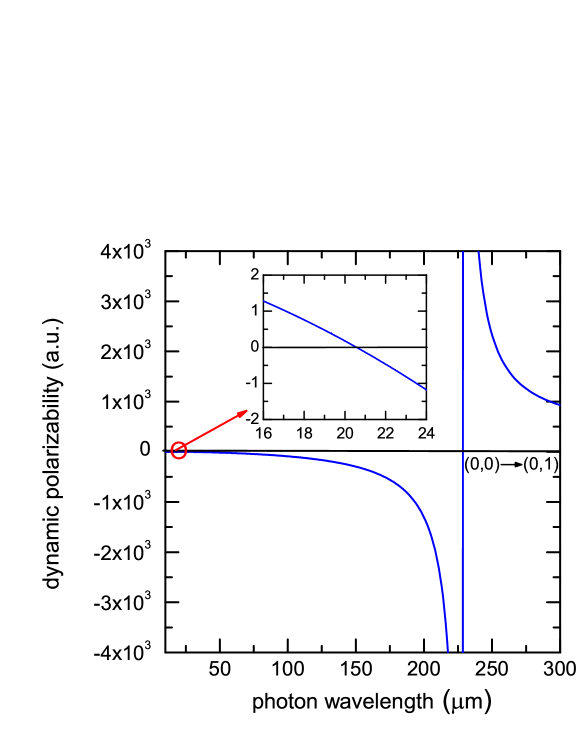
Figure 3: (Color online) Dynamic dipole polarizability $\alpha_{1}(\omega)$ (in a.u.) for the rovibronic ground-state $(\upsilon=0,L=0)$ of the HD⁺ ion for photon wavelengths from 10 to 300 $\mu\textrm{m}$. The $(0,0)\rightarrow(0,1)$ resonance in the dynamic polarizability is marked. The inset is a magnification of the circled position around 20 $\mu\textrm{m}$ where $\alpha_{1}(\omega)=0$.

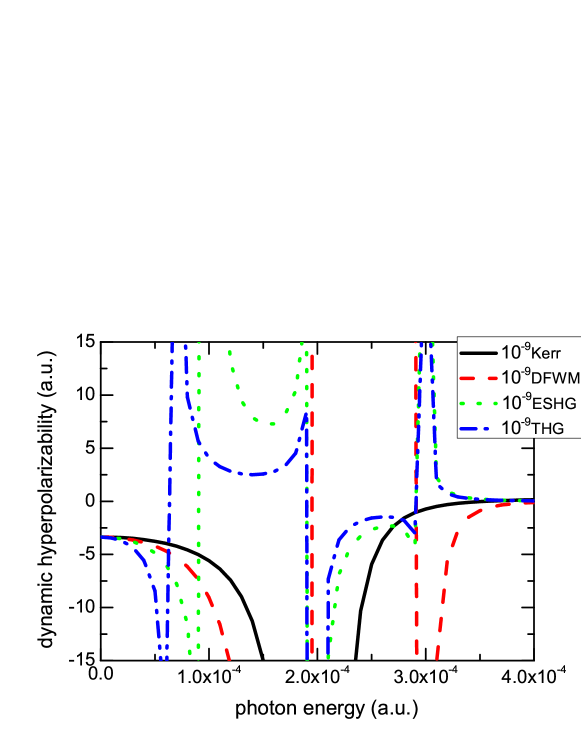
Figure 4: (Color online) Dynamic hyperpolarizabilities (in a.u.), see text, for the rovibronic ground-state $(\upsilon=0,L=0)$ of the HD⁺ ion for photon energies $\omega\leq 0.0004$ a.u. The solid black line represents the Kerr effect, the dashed red line denotes DFWM, the dotted green line represents ESHG, and the dash-dot blue line is THG.

III.4 First excited-state static polarizabilities and hyperpolarizabilities

Table 6: Convergence of static scalar and tensor dipole polarizabilities (in a.u.) for the first excited-state $(\upsilon=0,L=1)$ of the H${}_{2}^{+}$ ion.

($N_{S}$,$N_{P}$,$N_{(pp^{\prime})P}$,$N_{D}$)	$\alpha_{1}(S)$	$\alpha_{1}((pp^{\prime})P)$	$\alpha_{1}(D)$	$\alpha_{1}(0)$	$\alpha_{1}^{(T)}$(0)
(124,140,185,131)	0.650 846 694 354 224	0.599 484 436 191	1.903 824 885 459	3.154 156 016 01	$-$0.541 486 964 805
(175,205,255,295)	0.650 848 412 543 154	0.610 162 196 819	1.913 244 494 929	3.174 255 104 29	$-$0.537 091 763 627
(240,290,342,404)	0.650 848 769 703 336	0.612 800 029 560	1.913 969 508 078	3.177 618 307 34	$-$0.535 845 705 731
(420,532,448,561)	0.650 848 734 133 560	0.613 242 706 580	1.914 080 822 144	3.178 172 262 86	$-$0.535 635 463 058
(680,695,575,727)	0.650 848 734 170 854	0.613 340 747 207	1.914 098 088 958	3.178 287 570 34	$-$0.535 588 169 463
(1036,1120,725,954)	0.650 848 734 188 369	0.613 352 442 310	1.914 098 306 929	3.178 299 483 43	$-$0.535 582 343 726
(1255,1388,900,1225)	0.650 848 734 193 030	0.613 353 636 014	1.914 100 742 509	3.178 303 114 90	$-$0.535 581 990 437
(1504,1697,1102,1544)	0.650 848 734 193 204	0.613 353 828 247	1.914 100 852 289	3.178 303 414 73	$-$0.535 581 905 299
(1785,2050,1333,1915)	0.650 848 734 193 242	0.613 353 844 426	1.914 100 898 193	3.178 303 476 81	$-$0.535 581 901 799
(2100,2450,1595,2342)	0.650 848 734 193 251	0.613 353 845 680	1.914 100 900 765	3.178 303 480 64	$-$0.535 581 901 430
(2451,2900,1890,2829)	0.650 848 734 193 253	0.613 353 845 788	1.914 100 901 118	3.178 303 481 10	$-$0.535 581 901 411
Extrapolated				3.178 303 481(1)	$-$0.535 581 901 4(1)

Table 6 shows a convergence study of the static scalar and tensor dipole polarizabilities for H${}_{2}^{+}$ in the rovibronic excited-state $(\upsilon=0,L=1)$. The integer $N_{(pp^{\prime})P}$ represents the number of intermediate states used when the electron and one nucleus are both in excited states of $p$ symmetry to form the total angular momentum $L=1$. The contribution of the configuration $\alpha_{1}((pp^{\prime})P)$ to $\alpha_{1}(0)$ is about 20%, as shown in Table 6. The final static scalar and tensor dipole polarizabilities are both converged to the ninth figures. Calculations of $\alpha_{1}(0)$ for $\textrm{D}_{2}^{+}$ were also carried out with similar results. Results for the static scalar and tensor dipole polarizabilities for HD⁺ are presented in Table 7 and there is a partial cancellation between two intermediate symmetries, which can be seen by comparing columns 2 and 4. For the largest basis set, $\alpha_{1}(S)=-130.024\,382\,526\,724$ a.u and $\alpha_{1}(D)=133.405\,246\,966\,154$ a.u.; thus, when the two terms are added a loss of two significant figures results. Similar calculations were performed to obtain the static multipole polarizabilities $\alpha_{2}(0)$ and $\alpha_{3}(0)$ of the H${}_{2}^{+}$, D${}_{2}^{+}$, and HD⁺ ions in their first excited-states $(\upsilon=0,L=1)$. Our results for $\alpha_{1}(0)$ and $\alpha_{1}^{(T)}(0)$ for all three molecular ions are in agreement with the recent results of Schiller et al Schiller et al. (2014b), which are accurate to 8 significant digits.

Table 7: Convergence of static scalar and tensor dipole polarizabilities (in a.u.) for HD⁺ in the rovibronic excite-state $(\upsilon=0,L=1)$.

($N_{S}$,$N_{P}$,$N_{(pp^{\prime})P}$,$N_{D}$)	$\alpha_{1}(S)$	$\alpha_{1}((pp^{\prime})P)$	$\alpha_{1}(D)$	$\alpha_{1}(0)$	$\alpha_{1}^{(T)}$(0)
(124,140,104,150)	-130.074 770 552 639	0.547 263 971 717	133.368 575 021 506	3.841 068 441	117.011 545 036
(240,290,221,325)	-130.024 339 444 310	0.600 501 791 517	133.405 220 142 988	3.981 382 490	116.984 068 326
(420,532,406,616)	-130.027 278 013 066	0.600 795 791 278	133.404 624 757 699	3.978 142 536	116.987 213 433
(680,890,675,815)	-130.024 394 969 388	0.608 486 409 588	133.405 156 819 278	3.989 248 259	116.988 122 492
(1036,1388,1044,1055)	-130.024 382 831 359	0.609 081 936 428	133.405 235 157 018	3.989 934 262	116.988 400 284
(1504,1697,1271,1340)	-130.024 382 564 424	0.609 175 971 976	133.405 245 134 960	3.990 038 543	116.988 446 037
(1785,2050,1529,1674)	-130.024 382 532 136	0.609 261 536 706	133.405 246 685 012	3.990 125 689	116.988 488 632
(2100,2450,1820,2061)	-130.024 382 527 321	0.609 275 874 989	133.405 246 931 565	3.990 140 279	116.988 495 772
(2451,2900,2299,2505)	-130.024 382 526 724	0.609 281 615 158	133.405 246 966 154	3.990 146 055	116.988 498 638
Extrapolated				3.990 148(2)	116.988 499(1)

Table 8: Static polarizabilities and hyperpolarizabilities (in a.u.) of H${}_{2}^{+}$, HD⁺, and D${}_{2}^{+}$ ions in the first excited-state $(\upsilon=0,L=1)$. The numbers in parentheses represent the computational uncertainties. The numbers in the square brackets denote powers of ten.

System	$\alpha_{1}(0)$	$\alpha_{1}^{(T)}(0)$	$\alpha_{2}(0)$	$\alpha_{3}(0)$
H${}_{2}^{+}$	3.178 303 481(1)	$-$0.535 581 901 4(1)	505.648 042 6(1)	24.076 096(1)
	3.178 303 479
D${}_{2}^{+}$	3.076 590 373(1)	$-$0.505 301 361 2(1)	942.776 985 8(1)	22.938 665(1)
HD+	3.990 148(2)	116.988 499(1)	751.719 465 6(3)	1265.003 2(2)
	3.990 667
System	$\gamma_{0}(0)$	$\gamma_{2}(0)$
H${}_{2}^{+}$	4580.48(3)	$-$835.88(2)
D${}_{2}^{+}$	7486.2986(1)	$-$1228.7041(1)
HD+	1.0708026(2)[9]	$-$1.1823956(1)[9]

Table 8 summarizes the final values of the static multipole polarizabilities and hyperpolarizabilities for the H${}_{2}^{+}$, D${}_{2}^{+}$ and HD⁺ ions in their first excited-states $(\upsilon=0,L=1)$. From this table, we can see that dipolar and octupolar quantities for HD⁺ are much larger than those for H${}_{2}^{+}$ and D${}_{2}^{+}$, especially for the hyperpolarizability, due to the allowed low-lying virtual state entering in the $\mbox{HD}^{+}$ case. For $\mbox{HD}^{+}(0,1)$, Moss and Valenzano Moss and Valenzano (2002) found $\alpha_{1}(0)=3.990\,667$ in a nonadiabatic calculation. For $\mbox{H}_{2}^{+}(0,1)$, Bishop and Lam Bishop and Lam (1988) find $\gamma_{0}=4\,634.39$ in the Born-Oppenheimer approximation.

III.5 Static Stark shift

The static Stark shift $\Delta E$ for the rovibronic ground-state $(0,0)$ of a hydrogen molecular ion in an electric field of strength ${\cal{E}}$ is

$$\Delta E=-\frac{{\cal{E}}^{2}}{2}\alpha_{1}(0)-\frac{{\cal{E}}^{4}}{24}\gamma_{0}(0;0,0,0)$$ (17)

and the relative ratio between the second term and the first term is written as

$$X=\frac{\gamma_{0}(0;0,0,0){\cal{E}}^{2}}{12\alpha_{1}(0)}.$$ (18)

This ratio determines the extent to which the Stark shift is influenced by the hyperpolarizability at high field strengths. Using the values of Table 3, at ${\cal{E}}=6.67\times 10^{-5}$ a.u. $\sim(334\;\textrm{kV/cm})$, we find $X=1.3\times 10^{-6}$ for H${}_{2}^{+}$, $X=2.4\times 10^{-6}$ for D${}_{2}^{+}$, and $X=-0.0031$ for HD⁺. When ${\cal{E}}=2.11\times 10^{-4}$ a.u. $\sim(1087\;\textrm{kV/cm})$, we find $X=1.3\times 10^{-5}$ for H${}_{2}^{+}$, $X=2.4\times 10^{-5}$ for D${}_{2}^{+}$, and $X=-0.032$ for HD⁺. So the hyperpolarizability effect is more significant for the HD⁺ system compared to either the H${}_{2}^{+}$ or D${}_{2}^{+}$ system. In particular, it can cancel the Stark shift from the dipole polarizabilities.

The leading term of static Stark shift $\Delta E$ for the transition $(0,0)\rightarrow(0,1)$ of hydrogen molecular ions in the electric field strength ${\cal{E}}$ is

$$\Delta E=-\frac{{\cal{E}}^{2}}{2}\big{[}\alpha_{1}^{(0,0)}(0)-\alpha_{1}^{(0,1)}(0)\big{]},$$ (19)

where $\alpha_{1}^{(0,0)}(0)$ and $\alpha_{1}^{(0,1)}(0)$ represent the static dipole polarizabilities for the ground-state $(0,0)$ and excited-state (0,1) respectively. Using the present values from Tables 3 and 8, we obtain $\Delta\alpha_{1}(0)=\alpha_{1}^{(0,0)}(0)-\alpha_{1}^{(0,1)}(0)=-0.009\,577\,675\,711$ a.u. for H${}_{2}^{+}$, $\Delta\alpha_{1}(0)=-0.004\,601\,675\,812$ a.u. for D${}_{2}^{+}$, and $\Delta\alpha_{1}(0)=391.316\,177\,674\,2$ a.u. for HD⁺. Thus the second-order Stark shift will be larger for HD⁺ than for either the H${}_{2}^{+}$ or D${}_{2}^{+}$ ion.

III.6 Tune-out and magic wavelengths of HD⁺

At certain laser frequencies where the dynamic polarizability vanishes it may be possible to eliminate the shift induced by an applied laser field LeBlanc and Thywissen (2007)—these frequencies are known as tune-out frequencies or wavelengths. In addition, there might exist laser frequencies for an ion in two different states where the radiation induced shifts are equal (because the dynamic polarizabilities are equal at those frequencies): These frequencies are known as magic frequencies or wavelengths.

For the first excited-state $(0,1)$ of HD⁺, the dynamic dipole polarizability is

$$\alpha_{1,M}(\omega)=\alpha_{1}(\omega)+\alpha_{1}^{T}(\omega)\frac{3M^{2}-L(L+1)}{L(2L-1)},$$ (20)

where $M$ is the magnetic quantum number. In Table 9 we list some of low-lying (in energy) tune-out wavelengths for the ground state and the first excited state of HD⁺. The positions of magic-wavelengths between the ground-state and the first excited-state of HD⁺ are marked by the arrows in Figs. 5–7, there are no magic-wavelengths in the visible light range. In Table 10 we list the values of the magic wavelengths indicated in Figs. 5–7.

Table 9: Tune-out wavelengths (in a.u.) for HD⁺. The numbers in parentheses represent the computational uncertainties.

State	$M$	Tune-out wavelengths
$(0,0)$	0	0.002 215 386 568(1)	0.009 036 752 923(1)	0.017 178 225 41(1)
$(0,1)$	0	0.001 578 607 28(1)	0.008 614 811 326(1)	0.009 169 305 51(1)	0.017 340 149(5)
$(0,1)$	$\pm$ 1	0.002 687 162(4)	0.009 174 487 6(3)	0.017 340 401(5)

Figure 5: (Color online) Dynamic dipole polarizabilities $\alpha_{1}(\omega)$ (in a.u.) of HD⁺ for photon energies between 0.0005 and 0.001 a.u. The solid black line denotes the dynamic polarizabilities of ground state $(\upsilon=0,L=0)$. The dashed red and dotted blue lines represent the dynamic polarizabilities of the first excited state$(\upsilon=0,L=1)$ with $M=0$ and $|M|=1$ respectively. The magic-wavelength for the transition $(0,0)\rightarrow(0,1)$ is marked by the arrow.

Figure 6: (Color online) As for Fig. 5, but for photon energies between 0.007 and 0.01 a.u.

Figure 7: (Color online) As for Fig. 5, but for photon energies between 0.016 and 0.018 a.u.

Table 10: Magic wavelengths expressed as photon energies (in a.u.) between the ground-state and the first excied-state of HD⁺ molecular ions. The values correspond to the marked arrows in Figs. 5–7. The number in parentheses represents the computational uncertainty.

$M$	Magic-wavelengths
0	0.000 768 659 980(1)	0.009 260 494 92(1)	0.016 800 815 862(5)	0.017 170 143 339(1)	0.017 343 53(1)
$\pm 1$	0.017 189 146 9(2)	0.017 331 08(1)

III.7 Long-range interactions

Table 11: Long-range dispersion coefficients $C_{6}$, $C_{8}$ and $C_{10}$ (in a.u.) for a ground state H${}_{2}^{+}$, D${}_{2}^{+}$, or HD⁺ ion interacting with a ground-state H, He, or Li atom. The numbers in parentheses represent the computational uncertainties.

System	$C_{6}$	$C_{8}$	$C_{10}$
H${}_{2}^{+}$-H	4.891 143 017 14(1)	90.316 962 31(1)	1807.210 076(2)
D${}_{2}^{+}$-H	4.797 060 197 49(1)	87.850 021 22(1)	1756.323 945(2)
HD+-H	5.381 569 069 96(1)	99.592 513 40(2)	2023.687 265(3)
H${}_{2}^{+}$-He	2.195 917 825 1(1)	28.404 530 92(1)	368.784 69(1)
D${}_{2}^{+}$-He	2.161 390 926 5(1)	27.641 661 03(1)	357.632 88(1)
HD+-He	2.344 144 702 7(3)	31.043 628 96(3)	416.428 89(1)
H${}_{2}^{+}$-Li	47.684(2)	2838.66(3)	168607(1)
D${}_{2}^{+}$-Li	46.411(2)	2754.84(2)	163881(1)
HD+-Li	66.498(2)	3354.24(2)	196257(1)

Spectroscopic measurements of the Rydberg states of the hydrogen molecules $\textrm{H}_{2}$ and $\textrm{D}_{2}$ have been performed by several groups Herzberg and Jungen (1982); Sturrus et al. (1991); Davies et al. (1990a); Osterwalder et al. (2004). The data can be explained in terms of the long-range polarization potential model, in which, among other terms, the multipole polarizabilities of the parent molecular ions $\textrm{H}_{2}^{+}$ or $\textrm{D}_{2}^{+}$ enter as parameters in the effective potentials of the multipole expansion of the ion interaction with the distant charge Herzberg and Jungen (1982); Chang et al. (1984); Sturrus et al. (1988). An elaborate polarization potential model was developed for analysis of experiments on the highly-excited Rydberg states of the hydrogen and deuterium molecules Sturrus (1988); Jungen et al. (1989); Davies et al. (1990b); Sturrus et al. (1991); Jacobson et al. (1997, 2000). Its application yielded the experimental values for the static polarizabilities Jacobson et al. (2000) given in Table 3. Our nonadiabatic results for $\alpha_{2}(0)$ and higher multipoles do not appear to be readily applicable to this particular model, which utilizes a separation of higher order polarizabilities into electronic, vibrational, and rotational contributions. For example, fits of the measured spectra utilize the electronic and vibrational components of $\alpha_{2}(0)$; the rotational component is treated as a higher order perturbation Sturrus (1988); Jacobson et al. (1997) and handled separately.

We used the dynamic multipole polarizabilities to calculate the long-range dispersion coefficients $C_{6}$, $C_{8}$, and $C_{10}$ for the interaction between a ground state H, He, or Li atom and a ground state $\textrm{H}_{2}^{+}$, $\textrm{D}_{2}^{+}$, or $\textrm{HD}^{+}$ ion. The results are given in Table 11. The detailed expressions for the coefficients were given in Refs. Tang et al. (2009a) and Tang et al. (2009b). For the atoms we used methods described previously. For H, the energies and matrix elements are obtained using the Sturmian basis set to diagonalize the hydrogen Hamiltonian Yan et al. (1996), while for He and Li, the wave functions are expanded as a linear combination of Hylleraas functions Yan et al. (1996); Tang et al. (2009a).

When the atom is in the ground state but the molecular ion (denoted by “b”) is in an excited $L_{b}$ state with magnetic quantum number $M_{b}$, the leading terms of the second-order interaction energy are

$$V_{ab}=-\frac{C_{6}^{M_{b}}}{R^{6}}-\frac{C_{8}^{M_{b}}}{R^{8}}-\cdots,.$$ (21)

The detailed expressions for $C_{6}^{M_{b}}$ and $C_{8}^{M_{b}}$ are given in Refs. Tang et al. (2009a) and Tang et al. (2009b).

Table 12: Long-range dispersion coefficients $C_{6}^{M_{b}}$ and $C_{8}^{M_{b}}$ (in a.u.) for an H${}_{2}^{+}$, D${}_{2}^{+}$, or HD⁺ ion in the first excited-state with magnetic quantum number $M_{b}$ interacting with a ground-state H, He, or Li atom. The numbers in parentheses represent the computational uncertainties.

System	$M_{b}$	$C_{6}^{M_{b}}$	$C_{8}^{M_{b}}$
H${}_{2}^{+}$-H	0	5.542 473 599 4(1)	114.730 417 8(1)
D${}_{2}^{+}$-H	0	5.417 791 267 5(1)	110.820 998 3(1)
HD+-H	0	6.233 633(2)	136.097 48(2)
H${}_{2}^{+}$-H	$\pm 1$	4.581 282 889 3(1)	71.564 803 4(1)
D${}_{2}^{+}$-H	$\pm 1$	4.494 441 451 7(1)	69.756 367 1(2)
HD+-H	$\pm 1$	4.968 859(2)	74.802 77(3)
H${}_{2}^{+}$-He	0	2.449 741 778 8(1)	36.967 531 92(1)
D${}_{2}^{+}$-He	0	2.404 518 138 9(2)	35.706 083 48(2)
HD+-He	0	2.659 058(1)	43.666 737(2)
H${}_{2}^{+}$-He	$\pm 1$	2.075 030 168 4(1)	20.670 396 1(1)
D${}_{2}^{+}$-He	$\pm 1$	2.042 792 749 7(1)	20.159 006 1(1)
HD+-He	$\pm 1$	2.191 658(1)	21.291 70(4)
H${}_{2}^{+}$-Li	0	55.361(1)	3500.16(2)
D${}_{2}^{+}$-Li	0	53.635(1)	3377.72(2)
HD+-Li	0	81.810(1)	4431.18(2)
H${}_{2}^{+}$-Li	$\pm 1$	44.045(1)	2466.08(1)
D${}_{2}^{+}$-Li	$\pm 1$	42.893(1)	2395.81(1)
HD+-Li	$\pm 1$	59.047(1)	2772.99(1)

Table 12 lists the dispersion coefficients of H${}_{2}^{+}$, D${}_{2}^{+}$, and HD⁺ ions in the first excited state $(L_{b}=1)$ interacting with the ground-state H, He, and Li atoms. As above, the atomic properties were taken from Ref. Yan et al. (1996). Note that the precision of the calculated $C_{6}^{M_{b}}$ and $C_{8}^{M_{b}}$ for the excited-state HD⁺ interacting with H and He atoms is less than that for the H${}_{2}^{+}$ and D${}_{2}^{+}$ ions. In the case of interactions with Li, the accuracy of the coefficients is limited by the accuracy of the Li calculations.

IV Conclusion

We calculated the static and dynamic multipole polarizabilities and hyerpolarizabilities for the ground and first excited states of H${}_{2}^{+}$, D${}_{2}^{+}$, and HD⁺ in the non-relativistic limit by using correlated Hylleraas basis sets without using the Born-Oppenheimer approximation. For the static dipole polarizability of H${}_{2}^{+}$, the present value is the most accurate to date. The hyperpolarizabilities were calculated without derivatives (not using finite field methods) for H${}_{2}^{+}$ and its isotopomers. The present high precision values can not only be taken as a benchmark for testing other theoretical methods, but may also lay a foundation for investigating the relativistic and QED effects on polarizabilites and hyperpolarizabilities and assist in planning experimental research on hydrogen molecular ions.