Spin density matrix elements in exclusive $\omega$ electroproduction on ¹H and ²H targets at 27.5 GeV beam energy

Abstract

Exclusive electroproduction of $\omega$ mesons on unpolarized hydrogen and deuterium targets is studied in the kinematic region of $Q^{2}>$ 1.0 GeV², 3.0 GeV $<W<$ 6.3 GeV, and $-t^{\prime}<$ 0.2 GeV². Results on the angular distribution of the $\omega$ meson, including its decay products, are presented. The data were accumulated with the HERMES forward spectrometer during the 1996-2007 running period using the 27.6 GeV longitudinally polarized electron or positron beam of HERA. The determination of the virtual-photon longitudinal-to-transverse cross-section ratio reveals that a considerable part of the cross section arises from transversely polarized photons. Spin density matrix elements are presented in projections of $Q^{2}$ or $-t^{\prime}$. Violation of $s$-channel helicity conservation is observed for some of these elements. A sizable contribution from unnatural-parity-exchange amplitudes is found and the phase shift between those amplitudes that describe transverse $\omega$ production by longitudinal and transverse virtual photons, $\gamma^{*}_{L}\to\omega_{T}$ and $\gamma^{*}_{T}\to\omega_{T}$, is determined for the first time. A hierarchy of helicity amplitudes is established, which mainly means that the unnatural-parity-exchange amplitude describing the $\gamma^{*}_{T}\to\omega_{T}$ transition dominates over the two natural-parity-exchange amplitudes describing the $\gamma^{*}_{L}\to\omega_{L}$ and $\gamma^{*}_{T}\to\omega_{T}$ transitions, with the latter two being of similar magnitude. Good agreement is found between the HERMES proton data and results of a pQCD-inspired phenomenological model that includes pion-pole contributions, which are of unnatural parity.

1 Introduction

Exclusive electroproduction of vector mesons on nucleons offers a rich source of information on the mechanisms that produce these mesons, see e.g., Refs. Fran ; diehl1 . This process can be considered to consist of three subprocesses: i) the incident lepton emits a virtual photon $\gamma^{*}$, which dissociates into a $q\bar{q}$ pair; ii) this pair interacts strongly with the nucleon; iii) from the scattered $q\bar{q}$ pair the observed vector meson is formed.

In Regge phenomenology, the interaction of the $q\bar{q}$ pair with the nucleon proceeds through the exchange of a pomeron or (a combination of) the exchanges of other reggeons (e.g., $\rho$, $\omega$, $\pi$, …). If the quantum numbers of the particle lying on the Regge trajectory are $J^{P}=0^{+},\;1^{-}$, …, the process is denoted Natural Parity Exchange (NPE). Alternatively, the case of $J^{P}=0^{-},\;1^{+}$, … is denoted Unnatural Parity Exchange (UPE). In perturbative quantum chromodynamics (pQCD), the interaction of the $q\bar{q}$ pair with the nucleon can proceed via two-gluon exchange or quark-antiquark exchange, where the former corresponds to the exchange of a pomeron and the latter to the exchange of a (combination of) reggeon(s).

Spin density matrix elements (SDMEs) describe the final spin states of the produced vector meson. In this work, SDME values will be determined and discussed in the formalism that was developed in Ref. Schill for the case of an unpolarized or longitudinally polarized beam and an unpolarized target. For completeness, we also present SDME values in the more general formalism of Ref. Diehl . The SDMEs can be expressed in terms of helicity amplitudes that describe the transitions from the initial helicity states of virtual photon and incoming nucleon to the final helicity states of the produced vector meson and the outgoing nucleon. The values of SDMEs will be used to establish a hierarchy of helicity amplitudes, to test the hypothesis of $s$-channel helicity conservation, to investigate UPE contributions, and to determine the longitudinal-to-transverse cross-section ratio.

In the framework of pQCD, the nucleon structure can also be studied through hard exclusive meson production as the process amplitude contains Generalized Parton Distributions (GPDs) gpd1 ; gpd2 ; gpd3 . For longitudinal virtual photons, this amplitude is proven to factorize rigorously into a perturbatively calculable hard-scattering part and two soft parts (collinear factorization) Radyushkin:1996ru ; Collins:1996fb . The soft parts of the convolution contain GPDs and a meson distribution amplitude. At leading twist, the chiral-even GPDs $H^{f}$ and $E^{f}$ are sufficient to describe exclusive vector-meson production on a spin-$1/2$ target such as a proton or a neutron, where $f$ denotes a quark of flavor $f$ or a gluon. These GPDs are of special interest as they are related to the total angular momentum carried by quarks or gluons in the nucleon Ji:1996e .

Although there is no such rigorous proof for transverse virtual photons, phenomenological models use the modified perturbative approach Botts:1989kf instead, which takes into account parton transverse momenta. The latter are included at subleading twist in the subprocess $\gamma^{*}f\rightarrow{\cal M}f$, where ${\cal M}$ denotes the meson, while the partons are still emitted and reabsorbed by the nucleon collinear to the nucleon momentum. By using this approach, the pQCD-inspired phenomenological “GK model” can describe existing data on cross sections, SDMEs and spin asymmetries in exclusive vector-meson production for values of Bjorken-$x$, $x_{B}$, below about 0.2 Goloskokov:2005sd ; Goloskokov:2007nt ; Goloskokov:2013mba . It can also describe exclusive leptoproduction of pseudoscalar mesons by including the full contribution to the electromagnetic form factor from the pion, in contrast to earlier studies at leading-twist, which took into account only the relatively small perturbative contribution to this form factor (see Ref. Goloskokov:2009ia and references therein). The GK model also applies successfully to the description of deeply virtual Compton scattering k_mo_sa . The results of the most recent variant of the GK model, in which the unnatural-parity contributions due to pion exchange are included to describe exclusive $\omega$ leptoproduction thcal , will be compared in this paper to the HERMES proton data in terms of SDMEs and certain combinations of them.

Early papers on exclusive $\omega$ electroproduction are summarized in Ref. Bauer , which particularly contains results on SDMEs obtained at DESY for 0.3 GeV² $<Q^{2}<$ 1.4 GeV² and 0.3 GeV $<W<$ 2.8 GeV. The symbol $Q^{2}$ represents the negative square of the virtual-photon four-momentum and $W$ is the invariant mass of the photon-nucleon system. Recently, SDMEs in exclusive $\omega$ electroproduction were studied for 1.6 GeV² $<Q^{2}<$ 5.2 GeV² by CLAS clas and it was found that the exchange of the pion Regge trajectory dominates exclusive $\omega$ production, even for Q² values as large as 5 GeV².

2 Formalism

2.1 Spin density matrix elements

The $\omega$ meson is produced in the following reaction:

$$e+p\to e+p+\omega,$$ (1)

with a branching ratio $Br=89.1\%$ for the $\omega$ decay:

$$\omega\to\pi^{+}+\pi^{-}+\pi^{0},~{}\pi^{0}\to 2\gamma.$$ (2)

The angular distribution of the three final-state pions depends on SDMEs. The first subprocess of vector-meson production, the emission of a virtual photon ($e\rightarrow e+\gamma^{*}$), is described by the photon spin density matrix Schill ,

$$\varrho^{U+L}_{\lambda_{\gamma}\lambda^{\prime}_{\gamma}}=\varrho^{U}_{\lambda_{\gamma}\lambda^{\prime}_{\gamma}}+P_{b}\varrho^{L}_{\lambda_{\gamma}\lambda^{\prime}_{\gamma}},$$ (3)

where U and L denote unpolarized and longitudinally polarized beam, respectively, and $P_{b}$ is the value of the beam polarization. The photon spin density matrix can be calculated in quantum electrodynamics.

The vector-meson spin density matrix $\rho_{\lambda_{V}\lambda_{V}^{{}^{\prime}}}$ is expressed through helicity amplitudes $F_{\lambda_{V}\lambda^{\prime}_{N}\lambda_{\gamma}\lambda_{N}}$. These amplitudes describe the transition of a virtual photon with helicity $\lambda_{\gamma}$ to a vector meson with helicity $\lambda_{V}$, while $\lambda_{N}$ and $\lambda^{\prime}_{N}$ are the helicities of the nucleon in the initial and final states, respectively. Helicity amplitudes depend on $W$, $Q^{2}$, and $t^{\prime}=t-t_{min}$, where $t$ is the Mandelstam variable and $-t_{min}$ represents the smallest kinematically allowed value of $-t$ at fixed virtual-photon energy and $Q^{2}$. The quantity $\sqrt{-t^{\prime}}$ is approximately equal to the transverse momentum of the vector meson with respect to the direction of the virtual photon in the $\gamma^{*}N$ centre-of-mass (CM) system. In this system, the spin density matrix of the vector meson is given by the von Neumann equation Schill ,

$$\rho_{\lambda_{V}\lambda^{\prime}_{V}}=\frac{1}{2\mathcal{N}}\sum_{\lambda_{\gamma}\lambda^{\prime}_{\gamma}\lambda_{N}\lambda^{\prime}_{N}}F_{\lambda_{V}\lambda^{\prime}_{N}\lambda_{\gamma}\lambda_{N}}\varrho^{U+L}_{\lambda_{\gamma}\lambda^{\prime}_{\gamma}}F_{\lambda^{\prime}_{V}\lambda^{\prime}_{N}\lambda^{\prime}_{\gamma}\lambda_{N}}^{*}\,,$$ (4)

where $\mathcal{N}$ is a normalization factor, see Refs. Schill ; DC-24 .

After the decomposition of $\varrho^{U+L}_{\lambda_{\gamma}\lambda^{\prime}_{\gamma}}$ into the standard set of $3\times 3$ Hermitian matrices $\Sigma^{\alpha}$, the vector-meson spin density matrix is expressed in terms of a set of nine matrices $\rho^{\alpha}_{\lambda_{V}\lambda^{\prime}_{V}}$ related to various photon polarization states: transversely polarized photon ($\alpha$=0,…,3), longitudinally polarized photon ($\alpha$=4), and terms describing their interference ($\alpha$=5,…,8) Schill . When contributions of transverse and longitudinal photons cannot be separated, the SDMEs are customarily defined as

$$r^{04}_{\lambda_{V}\lambda^{\prime}_{V}} =(\rho^{0}_{\lambda_{V}\lambda^{\prime}_{V}}+\epsilon R\rho^{4}_{\lambda_{V}\lambda^{\prime}_{V}})(1+\epsilon R)^{-1},$$

$$r^{\alpha}_{\lambda_{V}\lambda^{\prime}_{V}} =\begin{cases}{\rho^{\alpha}_{\lambda_{V}\lambda^{\prime}_{V}}}{(1+\epsilon R)^{-1}},\;\alpha=1,2,3,\\ {\sqrt{R}\rho^{\alpha}_{\lambda_{V}\lambda^{\prime}_{V}}}{(1+\epsilon R)^{-1}},\;\alpha=5,6,7,8.\end{cases}\hskip 7.11317pt$$ (5)

The quantity $R=d\sigma_{L}/d\sigma_{T}$ is the longitudinal-to-transverse virtual-photon differential cross-section ratio and $\epsilon$ is the ratio of fluxes of longitudinal and transverse virtual photons.

2.2 Helicity amplitudes

A helicity amplitude can be decomposed into a sum of a NPE amplitude T and a UPE amplitude U,

$$F_{\lambda_{V}\lambda^{\prime}_{N}\lambda_{\gamma}\lambda_{N}}=T_{\lambda_{V}\lambda^{\prime}_{N}\lambda_{\gamma}\lambda_{N}}+U_{\lambda_{V}\lambda^{\prime}_{N}\lambda_{\gamma}\lambda_{N}},$$ (6)

for details see Refs. Schill ; DC-24 . The relations between the amplitudes $F$, $T$, and $U$ are the following Schill :

$$T_{\lambda_{V}\lambda^{\prime}_{N}\lambda_{\gamma}\lambda_{N}}=\frac{1}{2}[F_{\lambda_{V}\lambda^{\prime}_{N}\lambda_{\gamma}\lambda_{N}}~{}~{}~{}~{}~{}~{}~{}~{}~{}~{}~{}~{}~{}~{}~{}~{}~{}~{}~{}~{}~{}~{}~{}~{}~{}~{}~{}$$

$$+(-1)^{\lambda_{V}-\lambda_{\gamma}}F_{-\lambda_{V}\lambda^{\prime}_{N}-\lambda_{\gamma}\lambda_{N}}],$$ (7)

$$U_{\lambda_{V}\lambda^{\prime}_{N}\lambda_{\gamma}\lambda_{N}}=\frac{1}{2}[F_{\lambda_{V}\lambda^{\prime}_{N}\lambda_{\gamma}\lambda_{N}}~{}~{}~{}~{}~{}~{}~{}~{}~{}~{}~{}~{}~{}~{}~{}~{}~{}~{}~{}~{}~{}~{}~{}~{}~{}~{}~{}$$

$$-(-1)^{\lambda_{V}-\lambda_{\gamma}}F_{-\lambda_{V}\lambda^{\prime}_{N}-\lambda_{\gamma}\lambda_{N}}].$$ (8)

The asymptotic behaviour of amplitudes $F$ at small $-t^{\prime}$ Diehl ,

$$F_{\lambda_{V}\lambda^{\prime}_{N}\lambda_{\gamma}\lambda_{N}}\propto\Bigl{(}\frac{\sqrt{-t^{\prime}}}{M}\Bigr{)}^{|(\lambda_{V}-\lambda^{\prime}_{N})-(\lambda_{\gamma}-\lambda_{N})|},$$ (9)

follows from angular-momentum conservation. Equations (7)-(9) show that the double-helicity-flip amplitudes with $|\lambda_{V}-\lambda_{\gamma}|=2$ are suppressed at least by a factor of $\sqrt{-t^{\prime}}/M$, and the contributions of these double-helicity-flip amplitudes to the SDMEs are suppressed by $-t^{\prime}/M^{2}$. Therefore they will be neglected throughout the paper.

For an unpolarized target, there exists no interference between NPE and UPE amplitudes and there is no linear contribution from nucleon-helicity-flip amplitudes to SDMEs. For brevity, the following notations will be used:

$$\widetilde{\sum}T_{\lambda_{V}\lambda_{\gamma}}T^{*}_{\lambda^{\prime}_{V}\lambda^{\prime}_{\gamma}}\equiv\frac{1}{2}\sum_{\lambda_{N}\lambda^{\prime}_{N}}T_{\lambda_{V}\lambda^{\prime}_{N}\lambda_{\gamma}\lambda_{N}}T^{*}_{\lambda^{\prime}_{V}\lambda^{\prime}_{N}\lambda^{\prime}_{\gamma}\lambda_{N}}.$$ (10)

Using the symmetry properties Schill ; DC-24 of the amplitudes $T$, Eq. (10) can be rewritten as

$$\widetilde{\sum}T_{\lambda_{V}\lambda_{\gamma}}T^{*}_{\lambda^{\prime}_{V}\lambda^{\prime}_{\gamma}}=~{}~{}~{}~{}~{}~{}~{}~{}~{}~{}~{}~{}~{}~{}~{}~{}~{}~{}~{}~{}~{}~{}~{}~{}~{}~{}~{}~{}~{}~{}~{}~{}~{}~{}~{}~{}~{}~{}~{}~{}~{}~{}~{}~{}$$

$$T_{\lambda_{V}\frac{1}{2}\lambda_{\gamma}\frac{1}{2}}T^{*}_{\lambda^{\prime}_{V}\frac{1}{2}\lambda^{\prime}_{\gamma}\frac{1}{2}}+T_{\lambda_{V}-\frac{1}{2}\lambda_{\gamma}\frac{1}{2}}T^{*}_{\lambda^{\prime}_{V}-\frac{1}{2}\lambda^{\prime}_{\gamma}\frac{1}{2}}.$$ (11)

Here, the first and second product on the right-hand side gives the contribution of NPE amplitudes without and with nucleon-helicity flip, respectively. Analogous relations hold for UPE amplitudes. An additional abbreviated notation in the text will be the omission of the nucleon-helicity indices when discussing the amplitudes with $\lambda_{N}=\lambda^{\prime}_{N}$, i.e.,

$$T_{\lambda_{V}\lambda_{\gamma}} \equiv T_{\lambda_{V}\frac{1}{2}\lambda_{\gamma}\frac{1}{2}}=T_{\lambda_{V}-\frac{1}{2}\lambda_{\gamma}-\frac{1}{2}}$$

$$U_{\lambda_{V}\lambda_{\gamma}} \equiv U_{\lambda_{V}\frac{1}{2}\lambda_{\gamma}\frac{1}{2}}=-U_{\lambda_{V}-\frac{1}{2}\lambda_{\gamma}-\frac{1}{2}}.$$ (12)

The dominance of diagonal $\gamma^{*}\to V$ transitions ($\lambda_{V}=\lambda_{\gamma}$) is called $s$-channel helicity conservation (SCHC).

2.3 Angular distribution

The SDMEs in exclusive electroproduction of $\omega$ mesons are determined using the process in Eq. (1). They are fitted as parameters of $\mathcal{W}^{U+L}(\Phi,\phi,\cos\Theta)$, which is the three-dimensional angular distribution, to the corresponding experimental distribution of the three pions originating from the $\omega$-meson decay. The angular distribution $\mathcal{W}^{U+L}(\Phi,\phi,\cos\Theta)$ is decomposed into $\mathcal{W}^{U}$ and $\mathcal{W}^{L}$, see Eq. (13), which are the respective distributions for unpolarized and longitudinally polarized beams. From the fit, 15 “unpolarized” SDMEs (see Eq. (14)) are extracted and additionally 8 “polarized” SDMEs (see Eq. (15)) from data collected with a longitudinally polarized beam.

$$\mathcal{W}^{U+L}(\Phi,\phi,\cos{\Theta})= \ \mathcal{W}^{U}(\Phi,\phi,\cos{\Theta})+P_{b}\mathcal{W}^{L}(\Phi,\phi,\cos{\Theta}),$$ (13)

$$\mathcal{W}^{U}(\Phi,\phi,\cos{\Theta})= \ \frac{3}{8\pi^{2}}\Bigg{[}\frac{1}{2}(1-r^{04}_{00})+\frac{1}{2}(3r^{04}_{00}-1)\cos^{2}{\Theta}-\sqrt{2}\mathrm{Re}\{r^{04}_{10}\}\sin 2\Theta\cos\phi-r^{04}_{1-1}\sin^{2}\Theta\cos 2\phi\hskip 28.45274pt$$

$$-\epsilon\cos 2\Phi\Big{(}r^{1}_{11}\sin^{2}\Theta+r^{1}_{00}\cos^{2}{\Theta}-\sqrt{2}\mathrm{Re}\{r^{1}_{10}\}\sin 2\Theta\cos\phi-r^{1}_{1-1}\sin^{2}\Theta\cos 2\phi\Big{)}$$

$$-\epsilon\sin 2\Phi\Big{(}\sqrt{2}\mathrm{Im}\{r^{2}_{10}\}\sin 2\Theta\sin\phi+\mathrm{Im}\{r^{2}_{1-1}\}\sin^{2}\Theta\sin 2\phi\Big{)}$$

$$+\sqrt{2\epsilon(1+\epsilon)}\cos\Phi\Big{(}r^{5}_{11}\sin^{2}{\Theta}+r^{5}_{00}\cos^{2}\Theta-\sqrt{2}\mathrm{Re}\{r^{5}_{10}\}\sin 2\Theta\cos\phi-r^{5}_{1-1}\sin^{2}\Theta\cos 2\phi\Big{)}$$

$$+\sqrt{2\epsilon(1+\epsilon)}\sin\Phi\Big{(}\sqrt{2}\mathrm{Im}\{r^{6}_{10}\}\sin 2\Theta\sin\phi+\mathrm{Im}\{r^{6}_{1-1}\}\sin^{2}\Theta\sin 2\phi\Big{)}\Bigg{]},$$ (14)

$$\mathcal{W}^{L}(\Phi,\phi,\cos\Theta)= \ \frac{3}{8\pi^{2}}\Bigg{[}\sqrt{1-\epsilon^{2}}\Big{(}\sqrt{2}\mathrm{Im}\{r^{3}_{10}\}\sin 2\Theta\sin\phi+\mathrm{Im}\{r^{3}_{1-1}\}\sin^{2}\Theta\sin 2\phi\Big{)}$$

$$+\sqrt{2\epsilon(1-\epsilon)}\cos\Phi\Big{(}\sqrt{2}\mathrm{Im}\{r^{7}_{10}\}\sin 2\Theta\sin\phi+\mathrm{Im}\{r^{7}_{1-1}\}\sin^{2}\Theta\sin 2\phi\Big{)}$$

$$+\sqrt{2\epsilon(1-\epsilon)}\sin\Phi\Big{(}r^{8}_{11}\sin^{2}\Theta+r^{8}_{00}\cos^{2}\Theta-\sqrt{2}\mathrm{Re}\{r^{8}_{10}\}\sin 2\Theta\cos\phi-r^{8}_{1-1}\sin^{2}\Theta\cos 2\phi\Big{)}\Bigg{]}.$$ (15)

Definitions of angles and reference frames are shown in Fig. 1. The directions of the axes of the hadronic CM system and of the $\omega$-meson rest frame follow the directions of the axes of the helicity frame Schill ; DC-24 ; joos .

The angle $\Phi$ between the $\omega$ production and the lepton scattering plane in the hadronic CM system is given by

$$\cos\Phi =\frac{(\vec{q}\times\vec{v})\cdot(\vec{k}\times\vec{k}^{\prime})}{|\vec{q}\times\vec{v}|\cdot|\vec{k}\times\vec{k}^{\prime}|},$$ (16)

$$\sin\Phi =\frac{[(\vec{q}\times\vec{v})\times(\vec{k}\times\vec{k}^{\prime})]\cdot\vec{q}}{|\vec{q}\times\vec{v}|\cdot|\vec{k}\times\vec{k}^{\prime}|\cdot|\vec{q}|}.$$ (17)

Here $\vec{k}$, $\vec{k^{\prime}}$, $\vec{q}=\vec{k}-\vec{k^{\prime}}$, and $\vec{v}$ are the three-momenta of the incoming and outgoing leptons, virtual photon, and $\omega$ meson respectively.

The unit vector normal to the decay plane in the $\omega$ rest frame is defined by

$$\vec{n}=\frac{\vec{p}_{\pi^{+}}\times\vec{p}_{\pi^{-}}}{|\vec{p}_{\pi^{+}}\times\vec{p}_{\pi^{-}}|},$$ (18)

where $\vec{p}_{\pi^{+}}$ and $\vec{p}_{\pi^{-}}$ are the three-momenta of the positive and negative decay pions in the $\omega$ rest frame.

The polar angle $\Theta$ of the unit vector $\vec{n}$ in the $\omega$-meson rest frame, with the $z$-axis aligned opposite to the outgoing nucleon momentum $\vec{p}^{\prime}$ and the $y$-axis directed along $\vec{p}^{\prime}\times\vec{q}$, is defined by

$$\cos\Theta =-\frac{\vec{p}^{\prime}\cdot\vec{n}}{|\vec{p}^{\prime}|},$$ (19)

while the azimuthal angle $\phi$ of the unit vector $\vec{n}$ is given by

$$\cos\phi =\frac{(\vec{q}\times\vec{p}^{\prime})\cdot(\vec{p}^{\prime}\times\vec{n})}{|\vec{q}\times\vec{p}^{\prime}|\cdot|\vec{p}^{\prime}\times\vec{n}|},$$ (20)

$$\sin\phi =-\frac{[(\vec{q}\times\vec{p}^{\prime})\times\vec{p}^{\prime}]\cdot(\vec{n}\times\vec{p}^{\prime})}{|(\vec{q}\times\vec{p}^{\prime})\times\vec{p}^{\prime}|\cdot|\vec{n}\times\vec{p}^{\prime}|}.$$ (21)

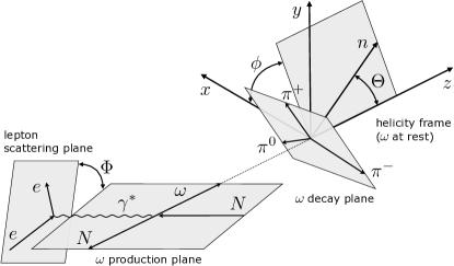
Figure 1: Definition of angles in the process $eN\to eN\omega$, where $\omega\to\pi^{+}\pi^{-}\pi^{0}$. Here, $\Phi$ is the angle between the $\omega$ production plane and the lepton scattering plane in the center-of-mass system of the virtual photon and the target nucleon. The variables $\Theta$ and $\phi$ are respectively the polar and azimuthal angles of the unit vector normal to the decay plane in the $\omega$-meson rest frame.

3 Data analysis

3.1 HERMES experiment

The data analyzed in this paper were accumulated with the HERMES spectrometer during the running period of 1996 to 2007 using the 27.6 GeV longitudinally polarized electron or positron beam of HERA, and gaseous hydrogen or deuterium targets. The HERMES forward spectrometer, which is described in detail in Ref. identif , was built of two identical halves situated above and below the lepton beam pipe. It consisted of a dipole magnet in conjunction with tracking and particle identification detectors. Particles were accepted when their polar angles were in the range $\pm 170$ mrad in the horizontal direction and $\pm(40-140)$ mrad in the vertical direction. The spectrometer permitted a precise measurement of charged-particle momenta, with a resolution of $1.5\%$. A separation of leptons was achieved with an average efficiency of $98\%$ and a hadron contamination below $1\%$.

3.2 Selection of exclusively produced $\omega$ mesons

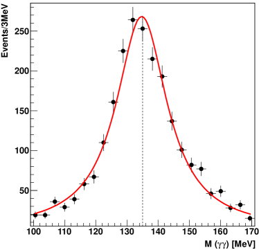
Figure 2: Two-photon invariant mass distribution after application of all criteria to select exclusively produced $\omega$ mesons. The Breit–Wigner fit to the mass distribution is shown as a continuous line and the dashed line indicates the PDG value of the $\pi^{0}$ mass.

The following requirements were applied to select exclusively produced $\omega$ mesons from reaction (1):
i) Exactly two oppositely charged hadrons, which are assumed to be pions, and one lepton with the same charge as the beam lepton are identified through the analysis of the combined responses of the four particle-identification detectors identif .
ii) A $\pi^{0}$ meson that is reconstructed from two calorimeter clusters as explained in Ref. arny is selected requiring the two-photon invariant mass to be in the interval $0.11$ GeV $<M({\gamma\gamma})<$ 0.16 GeV. The distribution of $M({\gamma\gamma})$ is shown in Fig. 2. This distribution is centered at $m_{\pi^{0}}=134.69\pm 19.94$ MeV, which agrees well with the PDG pdg value of the $\pi^{0}$ mass.
iii) The three-pion invariant mass is required to obey 0.71 GeV$\leq M(\pi^{+}\pi^{-}\pi^{0})\leq$ 0.87 GeV.
iv) The kinematic requirements for exclusive production of $\omega$ mesons are the following:
a) The scattered-lepton momentum lies above $3.5$ GeV.
b) The constraint $-t^{\prime}<$ 0.2 GeV² is used.
c) For exclusive production the missing energy $\Delta E$ must vanish. Here, the missing energy is calculated both for proton and deuteron as $\Delta E=\frac{M^{2}_{X}-M^{2}_{p}}{2M_{p}}$, with $M_{p}$ being the proton mass and $M^{2}_{X}=({p}+{q}-{p}_{\pi^{+}}-{p}_{\pi^{-}}-{p}_{\pi^{0}})^{2}$ the missing mass squared, where ${p}$, ${q}$, ${p}_{\pi^{+}}$, ${p}_{\pi^{-}}$, and ${p}_{\pi^{0}}$ are the four-momenta of target nucleon, virtual photon, and each of the three pions respectively. In this analysis, taking into account the spectrometer resolution, the missing energy has to lie in the interval $-1.0$ GeV $<\Delta E<0.8$ GeV, which is referred to as “exclusive region” in the following.
d) The requirement $Q^{2}>$ 1.0 GeV² is applied in order to facilitate the application of pQCD.
e) The requirement $W>3.0$ GeV is applied in order to be outside of the resonance region, while an upper cut of $W<6.3$ GeV is applied in order to define a clean kinematic phase space.

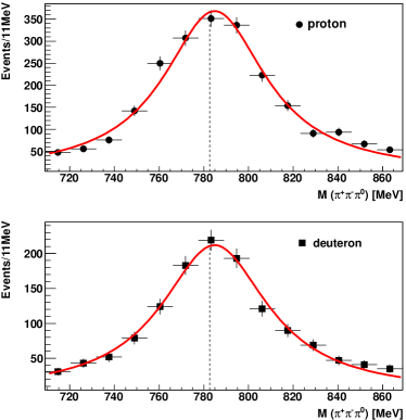
Figure 3: Breit-Wigner fit (solid line) of $\pi^{+}\pi^{-}\pi^{0}$ invariant mass distributions after application of all criteria to select $\omega$ mesons produced exclusively from proton (top) and from deuteron (bottom). The dashed line represents the PDG value of the $\omega$ mass.

After application of all these constraints, the proton sample contains 2260 and the deuteron sample 1332 events of exclusively produced $\omega$ mesons. These data samples are referred to in the following as data in the “entire kinematic region”. The invariant-mass distributions for exclusively produced $\omega$ mesons are shown in Fig. 3. Note the reasonable agreement of the fit result, $m_{\omega}=784.8\pm 55.8$ MeV for proton data and $m_{\omega}=784.6\pm 58.2$ MeV for deuteron data, with the PDG pdg value of the $\omega$ mass. The distributions of missing energy $\Delta$E, shown in Fig. 4, exhibit clearly visible exclusive peaks. The shaded histograms represent semi-inclusive deep-inelastic scattering (SIDIS) background obtained from a PYTHIA pythia Monte Carlo simulation that is normalized to data in the region $2~{}\text{GeV}<\Delta E<20~{}\text{GeV}$. The simulation is used to determine the fraction of background under the exclusive peak, which is calculated as the ratio of number of background events to the total number of events. It amounts to about 20% for the entire kinematic region and increases from 16% to 26% with increasing $-t^{\prime}$.

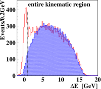
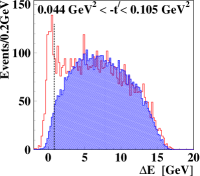
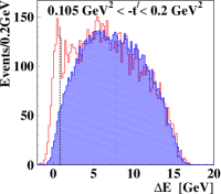
Figure 4: The $\Delta E$ distributions of $\omega$ mesons produced in the entire kinematic region and in three kinematic bins in $-t^{\prime}$ are compared with SIDIS $\Delta E$ distributions from PYTHIA (shaded area). The vertical dashed line denotes the upper limit of the exclusive region.

3.3 Comparison of data and Monte Carlo events

Distributions of experimental data in some kinematic variables are compared to those simulated by PYTHIA. The comparison is shown in Fig. 5 and mostly demonstrates good agreement between experimental and simulated data.

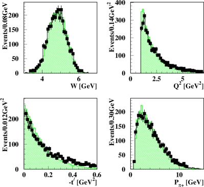
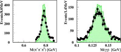
Figure 5: Distributions of several kinematic variables from experimental data on exclusive $\omega$-meson leptoproduction (black squares) in comparison with simulated exclusive events from the PYTHIA generator (dashed areas). Simulated events are normalized to the experimental data.

4 Extraction of $\omega$ spin density matrix elements

4.1 The unbinned maximum likelihood method

The SDMEs are extracted from data by fitting the angular distribution $\mathcal{W}^{U+L}(\Phi,\phi,\cos{\Theta})$ to the experimental angular distribution using an unbinned maximum likelihood method. The probability distribution function is $\mathcal{W}^{U+L}({\cal R};\Phi,\phi,\cos{\Theta})$, where ${\cal R}$ represents the set of 23 SDMEs, i.e., the coefficients of the trigonometric functions in Eqs. (14, 15). The negative log-likelihood function to be minimized reads

$$-\ln L({\cal R})=-\sum_{i=1}^{N}\ln\frac{\mathcal{W}^{U+L}({\cal R};\Phi_{i},\phi_{i},\cos{\Theta_{i}})}{\widetilde{\mathcal{N}}({\cal R})},$$ (22)

where the normalization factor

$$\widetilde{\mathcal{N}}({\cal R})=\sum_{j=1}^{N_{MC}}\mathcal{W}^{U+L}({\cal R};\Phi_{j},\phi_{j},\cos{\Theta_{j}})$$ (23)

is calculated numerically using events from a PYTHIA Monte Carlo generated according to an isotropic three-dimensional angular distribution and passed through the same analytical process as experimental data. The numbers of data and Monte Carlo events are denoted by ${N}$ and $N_{MC}$, respectively.

4.2 Background treatment

In order to account for the SIDIS background in the fit, first “SIDIS-background SDMEs” are obtained using Eqs. (22, 23) for the PYTHIA SIDIS sample in the exclusive region. Then, SDMEs corrected for SIDIS background are obtained as follows phdami :

$$-\ln L({\cal R})=~{}~{}~{}~{}~{}~{}~{}~{}~{}~{}~{}~{}~{}~{}~{}~{}~{}~{}~{}~{}~{}~{}~{}~{}~{}~{}~{}~{}~{}~{}~{}~{}~{}~{}~{}~{}~{}~{}~{}~{}~{}~{}~{}~{}~{}~{}~{}~{}~{}~{}~{}$$

$$-\sum_{i=1}^{N}\ln\Bigl{[}\frac{(1-f_{bg})*\mathcal{W}^{U+L}({\cal R};\Phi_{i},\phi_{i},\cos\Theta_{i})}{\widetilde{\mathcal{N}}({\cal R},\Psi)}$$

$$+\frac{f_{bg}*\mathcal{W}^{U+L}(\Psi;\Phi_{i},\phi_{i},\cos\Theta_{i})}{\widetilde{\mathcal{N}}({\cal R},\Psi)}\Bigr{]}.~{}~{}~{}$$ (24)

From now on, ${\cal R}$ denotes the set of SDMEs corrected for background, $\Psi$ the set of the SIDIS-background SDMEs, and $f_{bg}$ is the fraction of SIDIS background. The normalization factor reads correspondingly

$$\widetilde{\mathcal{N}}({\cal R},\Psi)=\sum_{j=1}^{N_{MC}}\left[(1-f_{bg})*\mathcal{W}^{U+L}({\cal R};\Phi_{j},\phi_{j},\cos\Theta_{j})\right.$$

$$\left.+f_{bg}*\mathcal{W}^{U+L}(\Psi;\Phi_{j},\phi_{j},\cos\Theta_{j})\right].~{}~{}~{}$$ (25)

4.3 Systematic uncertainties

The total systematic uncertainty on a given extracted SDME $r$ is obtained by adding in quadrature the uncertainty from the background subtraction procedure, $\Delta r_{sys}^{bg}$, and the one due to the extraction method, $\Delta r_{sys}^{MC}$. The former uncertainty is assigned to be the difference between the SDME obtained with and without background correction. This conservative approach also covers the small uncertainty on the fraction of SIDIS background, $f_{bg}$. The uncertainty $\Delta r_{sys}^{MC}$ is estimated using the Monte Carlo data that were generated with an angular distribution determined by the set of SDMEs ${\cal R}$. The statistics of the Monte Carlo data exceed those of the experimental data by about a factor of six. The generated events were passed through a realistic model of the HERMES apparatus using GEANT geant and were then reconstructed and analyzed in the same way as experimental data. These Monte Carlo data were used to extract the SDME set ${\cal R}^{MC}$. In this way, effects from detector acceptance, efficiency, smearing, and misalignment are accounted for. Two uncertainties are considered to be responsible for the difference between input and output value of a given SDME $r$,

$$(r-r^{MC})^{2}=(\Delta r_{sys}^{MC})^{2}+(\Delta r_{stat}^{MC})^{2},$$ (26)

where $\Delta r_{stat}^{MC}$ is the statistical uncertainty of $r^{MC}$ as obtained in the fitting procedure that uses MINUIT minuit . From Eq. (26), $\Delta r_{sys}^{MC}$ is determined, using the convention that $\Delta r_{sys}^{MC}$ is set to zero if $[(r-r^{MC})^{2}-(\Delta r_{stat}^{MC})^{2}]$ is negative.

5 Results

The results on SDMEs in the Schilling-Wolf Schill representation are given in Tables 1-5 in Appendix B and in the Diehl Diehl representation in Table 6 in the same Appendix. The SDMEs for the entire kinematic region are discussed in Sect. 5.1, while their dependences on $Q^{2}$ and $-t^{\prime}$ are discussed in Sect. 5.3.

5.1 SDMEs for the entire kinematic region

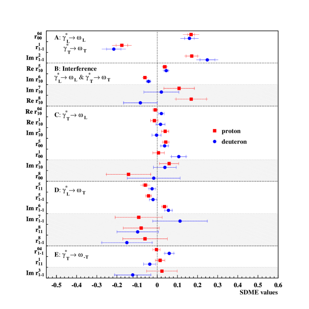
Figure 6: The 23 SDMEs for exclusive $\omega$ electroproduction extracted in the entire HERMES kinematic region with $\langle Q^{2}\rangle=2.42$ GeV², $\langle W\rangle=4.8$ GeV, $\langle-t^{\prime}\rangle=0.080$ GeV². Proton data are denoted by squares and deuteron data by circles. The inner error bars represent the statistical uncertainties, while the outer ones indicate the statistical and systematic uncertainties added in quadrature. Unpolarized (polarized) SDMEs are displayed in the unshaded (shaded) areas.

The SDMEs of the $\omega$ meson for the entire kinematic region ($\left<Q^{2}\right>=2.42$ GeV², $\left<W\right>=4.8$ GeV, and $\left<-t^{\prime}\right>=0.080$ GeV²) are presented in Fig. 6. These SDMEs are divided into five classes corresponding to different helicity transitions. The main terms in the expressions of class-A SDMEs correspond to the transitions from longitudinal virtual photons to longitudinal vector mesons, $\gamma^{*}_{L}\to V_{L}$, and from transverse virtual photons to transverse vector mesons, $\gamma^{*}_{T}\to V_{T}$. The dominant terms of class B correspond to the interference of these two transitions. The main terms of class-C, class-D, and class-E SDMEs are proportional to small amplitudes describing $\gamma^{*}_{T}\to V_{L}$, $\gamma^{*}_{L}\to V_{T}$, and $\gamma^{*}_{T}\to V_{-T}$ transitions respectively.
The SDMEs for the proton and deuteron data are found to be consistent with each other within their quadratically combined total uncertainties, with a $\chi^{2}$ per degrees of freedom of $28/23\approx 1.2$. In Fig. 6, the eight polarized SDMEs are presented in shaded areas. Their experimental uncertainties are larger in comparison to those of the unpolarized SDMEs because the lepton beam polarization is smaller than unity ($|P_{b}|\approx 40\%$) and in the equation for the angular distribution they are multiplied by the small kinematic factor $|P_{b}|\sqrt{1-\epsilon}\approx 0.2$, cf. Eq. (14) vs. Eq. (15).

5.2 Test of the SCHC hypothesis

In the case of SCHC, the seven SDMEs of class A and class B ($r_{00}^{04}$, $r_{1-1}^{1}$, $\mathrm{Im}\{r_{1-1}^{2}\}$, $\mathrm{Re}\{r_{10}^{5}\}$, $\mathrm{Im}\{r_{10}^{6}\}$, $\mathrm{Im}\{r_{10}^{7}\}$, $\mathrm{Re}\{r_{10}^{8}\}$) are not restricted to be zero, but six of them have to obey the following relations Schill :

$$r_{1-1}^{1} = -\mathrm{Im}\{r_{1-1}^{2}\},$$

$$\mathrm{Re}\{r_{10}^{5}\} = -\mathrm{Im}\{r_{10}^{6}\},$$

$$\mathrm{Im}\{r_{10}^{7}\} = \mathrm{Re}\{r_{10}^{8}\}.$$

The proton data yield

$$r^{1}_{1-1}+\mathrm{Im}\{r^{2}_{1-1}\} = -0.004\pm 0.038\pm 0.015,$$

$$\mathrm{Re}\{r^{5}_{10}\}+\mathrm{Im}\{r^{6}_{10}\} = -0.024\pm 0.013\pm 0.004,$$

$$\mathrm{Im}\{r^{7}_{10}\}-\mathrm{Re}\{r^{8}_{10}\} = -0.060\pm 0.100\pm 0.018,$$

and the deuteron data yield

$$r^{1}_{1-1}+\mathrm{Im}\{r^{2}_{1-1}\} = 0.033\pm 0.049\pm 0.016,$$

$$\mathrm{Re}\{r^{5}_{10}\}+\mathrm{Im}\{r^{6}_{10}\} = 0.001\pm 0.016\pm 0.005,$$

$$\mathrm{Im}\{r^{7}_{10}\}-\mathrm{Re}\{r^{8}_{10}\} = 0.104\pm 0.110\pm 0.023.$$

Here and in the following, the first uncertainty is statistical and the second systematic. In the calculation of the statistical uncertainty, the correlations between the different SDMEs are taken into account, see correlation matrices in Tables 8 and 9. It can be concluded that the above SCHC relations are fulfilled for class A and B. The SCHC relations for the class-A SDMEs $r^{1}_{1-1}$ and $\mathrm{Im}\{r^{2}_{1-1}\}$ can be violated only by the quadratic contributions of the double-helicity-flip amplitudes $T_{1\pm\frac{1}{2}-1\frac{1}{2}}$ and $U_{1\pm\frac{1}{2}-1\frac{1}{2}}$ with $|\lambda_{V}-\lambda_{\gamma}|=2$. The observed validity of SCHC means that their possible contributions are smaller than the experimental uncertainties. Also for class-B SDMEs, to which the same small double-helicity-flip amplitudes contribute linearly, no SCHC violation is observed. In addition, class-B SDMEs contain the contribution of the two small products $T_{0\pm\frac{1}{2}1\frac{1}{2}}T^{*}_{1\pm\frac{1}{2}0\frac{1}{2}}$ ($U_{0\pm\frac{1}{2}1\frac{1}{2}}U^{*}_{1\pm\frac{1}{2}0\frac{1}{2}}$). As the SCHC hypothesis is fulfilled, all these contributions are concluded to be negligibly small compared to the experimental uncertainties. This validates the assumption made in Sect. 2.2 that the double-helicity-flip amplitudes can be neglected.

All SDMEs of class C to E have to be zero in the case of SCHC. The class-C SDME $r^{5}_{00}$ deviates from zero by about three standard deviations for the proton and two standard deviations for the deuteron (see Fig. 6). Since the numerator of the equation for $r_{00}^{5}$ DC-24 ,

$$r^{5}_{00}=\frac{\mathrm{Re}\left\{T_{0-\frac{1}{2}1\frac{1}{2}}T^{*}_{0-\frac{1}{2}0\frac{1}{2}}+T_{0\frac{1}{2}1\frac{1}{2}}T^{*}_{0\frac{1}{2}0\frac{1}{2}}\right\}}{\cal{N}},$$ (27)

contains two amplitude products, at least one product is nonzero. However, without an amplitude analysis of the presented data it cannot be concluded which contribution to $r^{5}_{00}$ dominates. Both amplitudes $T_{0-\frac{1}{2}1\frac{1}{2}}$ and $T_{0\frac{1}{2}1\frac{1}{2}}$ have to be zero if the SCHC hypothesis holds.

Figure 6 shows that out of the six SDMEs of class D three, i.e., $r_{11}^{5}$, $r_{1-1}^{5}$, and $\mathrm{Im}\{r_{1-1}^{6}\}$, slightly differ from zero (see Table 1). As will be discussed in Sections 5.4 and 5.8, the largest UPE amplitudes in $\omega$ production are $U_{11}$ and $U_{10}$, and $|U_{11}|\gg|U_{10}|$. The main term of the first two SDMEs is proportional to $\mathrm{Re}[U_{10}U_{11}^{*}]$, while $\mathrm{Im}\{r_{1-1}^{6}\}$ is proportional to $-\mathrm{Re}[U_{10}U_{11}^{*}]$. The calculated linear combination of these three SDMEs, $r_{11}^{5}+r_{1-1}^{5}-\mathrm{Im}\{r_{1-1}^{6}\}$, is $-0.14\pm 0.03\pm 0.04$ for the proton and $-0.10\pm 0.03\pm 0.03$ for the deuteron. These values differ from zero by about three standard deviations of the total uncertainty for the proton. This, together with the experimental information on measured class-C and class-D SDMEs, indicates a violation of the SCHC hypothesis in exclusive $\omega$ production.

5.3 Dependences of SDMEs on $Q^{2}$ and $-t^{\prime}$ and comparison to a phenomenological model

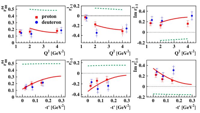
Figure 7: Q² and $-t^{\prime}$ dependences of class-A SDMEs. Proton data are denoted by squares and deuteron data by circles. Data points for deuteron data are slightly shifted horizontally for legibility. The representation of the uncertainties follows that of Fig. 6. The proton data are compared to calculations of a phenomenological model thcal , where solid (dashed) lines denote results with (without) pion-pole contributions.

In the following sections, kinematic dependences of the measured SDMEs and certain combinations of them are presented and interpreted wherever possible. In particular, the proton data presented in this paper are compared to the calculations of the phenomenological GK model described in Sect. 1. In each case, model calculations are shown with and without inclusion of the pion-pole contribution. In order to stay in the framework of handbag factorization and to avoid large $1/Q^{2}$ corrections, model calculations are only shown for $Q^{2}>2$ GeV², which leaves for the $Q^{2}$ dependence only two data points that can be compared to the model calculation. This paucity of comparable points makes it sometimes difficult to draw useful conclusions about the data-model comparison.

The kinematic dependences of SDMEs on $Q^{2}$ and $-t^{\prime}$ are presented in three bins of $Q^{2}$ with $\langle Q^{2}\rangle=1.28$ GeV², $\langle Q^{2}\rangle=2.00$ GeV², $\langle Q^{2}\rangle=4.00$ GeV², and $t^{\prime}$ with $\langle-t^{\prime}\rangle=0.021$ GeV², $\langle-t^{\prime}\rangle=0.072$ GeV², $\langle-t^{\prime}\rangle=0.137$ GeV². Table 7 shows the average value of $Q^{2}$ and $-t^{\prime}$ for bins in $-t^{\prime}$ and $Q^{2}$, respectively.

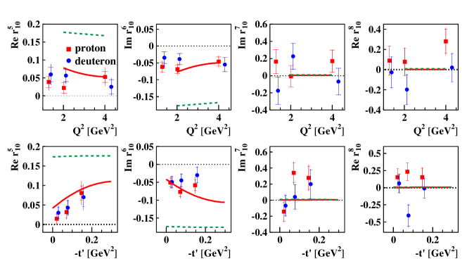
Figure 8: $Q^{2}$ and $-t^{\prime}$ dependences of class-B SDMEs. Otherwise as for Fig. 7.

The $Q^{2}$ and $-t^{\prime}$ dependences of class-A SDMEs are shown and compared to the model calculations in Fig. 7. All three SDMEs clearly show the need for the unnatural-parity contribution of the pion pole and the measured $-t^{\prime}$ dependence is well reproduced both in shape and magnitude. The same holds for the two unpolarized class-B SDMEs that are shown in Fig. 8. For the polarized class-B SDMEs as well as for all class-C SDMEs, which are shown in Fig. 9, the pion-pole contribution has little or no effect, and the model describes the magnitude of the data reasonably well. The class-D and E SDMEs are shown in Figs. 10 and 11, respectively. These SDMEs are expected to be zero if the pion-pole contribution is not included. When comparing the $-t^{\prime}$ dependences of the three unpolarized class-D SDMEs to the model calculation, also here the unnatural-parity pion-exchange contribution seems to be required. The two unpolarized class-E SDMEs are measured with reasonable precision, and agreement with the model calculation can be seen.

Within experimental uncertainties, the SDMEs measured on the proton are seen to be very similar to those measured on the deuteron. This can be understood by considering the different contributions to exclusive omega production. The pion-pole contribution is seen to be substantial thcal . For the NPE amplitudes, the dominant contribution comes from gluons and sea quarks, which are the same for protons and neutrons, while the valence-quark contribution is different. Thus altogether, only small differences between the proton and deuteron SDMEs are expected for incoherent scattering. As coherence effects are difficult to estimate, one can not exclude that they are of the size of the valence-quark effects. Therefore, the deuteron SDMEs are presently difficult to calculate reliably.

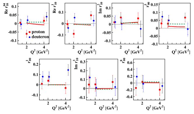
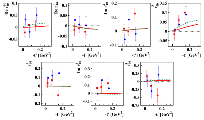
Figure 9: $Q^{2}$ and $-t^{\prime}$ dependences of class-C SDMEs. Otherwise as for Fig. 7.

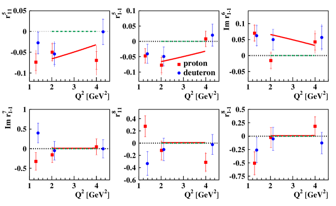
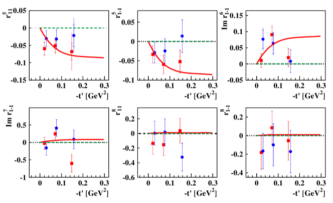
Figure 10: $Q^{2}$ and $-t^{\prime}$ dependences of class-D SDMEs. Otherwise as for Fig. 7.

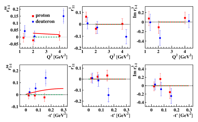
Figure 11: $Q^{2}$ and $-t^{\prime}$ dependences of class-E SDMEs. Otherwise as for Fig. 7.

5.4 UPE in $\omega$-meson production

In Fig. 12, the comparison of $\omega$ and $\rho^{0}$ DC-24 SDMEs is shown. One can see that the SDMEs $r^{1}_{1-1}$ and $\mathrm{Im}\{r^{2}_{1-1}\}$ of class A have opposite sign for $\omega$ and $\rho^{0}$. The SDME $r^{1}_{1-1}$ is negative for the $\omega$ meson and positive for $\rho^{0}$, while $\mathrm{Im}\{r^{2}_{1-1}\}$ is positive for $\omega$ and negative for $\rho^{0}$. In terms of helicity amplitudes, these two SDMEs are written DC-24 as

$$r_{1-1}^{1}=\frac{1}{2\mathcal{N}}\widetilde{\sum} \left(|T_{11}|^{2}+|T_{1-1}|^{2}\right.$$

$$\left.-|U_{11}|^{2}-|U_{1-1}|^{2}\right),$$ (28)

$$\mathrm{Im}\{r_{1-1}^{2}\}=\frac{1}{2\mathcal{N}}\widetilde{\sum} \left(-|T_{11}|^{2}+|T_{1-1}|^{2}\right.$$

$$\left.+|U_{11}|^{2}-|U_{1-1}|^{2}\right).$$ (29)

The difference between Eqs. (29) and (28) reads

$$\mathrm{Im}\{r_{1-1}^{2}\}-r_{1-1}^{1}=\frac{1}{\mathcal{N}}\widetilde{\sum}(-|T_{11}|^{2}+|U_{11}|^{2}).$$ (30)

For the entire kinematic region, this difference is clearly positive for the $\omega$ meson, hence $\widetilde{\sum}|U_{11}|^{2}>\widetilde{\sum}|T_{11}|^{2}$, while for the $\rho^{0}$ meson $\widetilde{\sum}|T_{11}|^{2}>\widetilde{\sum}|U_{11}|^{2}$ DC-24 . This suggests a large UPE contribution in exclusive $\omega$-meson production. Applying Eq. (11) to relation (30), the latter can be rewritten as

$$\mathrm{Im}\{r^{2}_{1-1}\}-r^{1}_{1-1}=\frac{1}{\mathcal{N}}( -|T_{1\frac{1}{2}1\frac{1}{2}}|^{2}-|T_{1-\frac{1}{2}1\frac{1}{2}}|^{2}$$

$$+|U_{1\frac{1}{2}1\frac{1}{2}}|^{2}+|U_{1-\frac{1}{2}1\frac{1}{2}}|^{2}).$$ (31)

The amplitudes with nucleon helicity flip, $T_{1-\frac{1}{2}1\frac{1}{2}}$ and $U_{1-\frac{1}{2}1\frac{1}{2}}$, should be zero at $t^{\prime}=0$ and are proportional to $\sqrt{-t^{\prime}}$ at small $t^{\prime}$ (see Eq. (9) and Ref. Diehl ). The small contribution of $|T_{1-\frac{1}{2}1\frac{1}{2}}|^{2}$ will be neglected from now on. As it was established above, the UPE contribution is larger than the NPE one. This means that if the dominant UPE helicity-flip amplitude is $U_{1-\frac{1}{2}1\frac{1}{2}}$, expression (31) would increase proportionally to $-t^{\prime}$. However, the experimental values of ($\mathrm{Im}\{r^{2}_{1-1}\}-r^{1}_{1-1}$) (see Tables 3 and 5) do not demonstrate such an increase; the values for the proton data even decrease smoothly with $-t^{\prime}$. Hence the dominant UPE amplitude is $U_{1\frac{1}{2}1\frac{1}{2}}$, and it holds $|U_{11}|^{2}>|T_{11}|^{2}$.

The existence of UPE in $\omega$ production on the proton and deuteron can also be tested with linear combinations of SDMEs such as

$$u_{1}=1-r^{04}_{00}+2r^{04}_{1-1}-2r^{1}_{11}-2r^{1}_{1-1},$$ (32)

$$u_{2}=r^{5}_{11}+r^{5}_{1-1},$$ (33)

$$u_{3}=r^{8}_{11}+r^{8}_{1-1}.$$ (34)

The quantity $u_{1}$ can be expressed in terms of helicity amplitudes as

$$u_{1}=\frac{1}{\mathcal{N}}\ \widetilde{\sum}{\left(4\epsilon|U_{10}|^{2}+2|U_{11}+U_{-11}|^{2}\right)}.$$ (35)

A non-zero result for $u_{1}$, implying that at least one of the four amplitudes $U_{1\pm\frac{1}{2}0\frac{1}{2}}$ or ($U_{1\pm\frac{1}{2}1\frac{1}{2}}+U_{-1\pm\frac{1}{2}1\frac{1}{2}}$) is nonzero, indicates the existence of UPE contributions. In the entire kinematic region, $u_{1}$ is 1.15 $\pm$ 0.09 $\pm$ 0.12 and 1.47 $\pm$ 0.12 $\pm$ 0.18 for proton and deuteron data, respectively. In Fig. 13, the $Q^{2}$ and $-t^{\prime}$ dependences of $u_{1}$ for proton and deuteron data are presented. It can be seen that $u_{1}$ is larger than unity, which implies the existence of large contributions from UPE transitions.

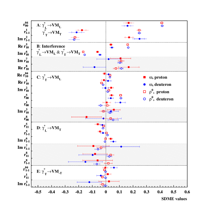
Figure 12: Comparison of SDMEs in exclusive $\omega$ and $\rho^{0}$ DC-24 electroproduction at HERMES for the entire kinematic region. The average values of the kinematic variables in exclusive $\rho^{0}$ production are $\langle Q^{2}\rangle=1.95$ GeV², $\langle W\rangle=4.8$ GeV, and $\langle-t^{\prime}\rangle=0.13$ GeV².

The expression for the quantities $u_{2}$ and $u_{3}$ in terms of helicity amplitudes is

$$u_{2}+iu_{3}=\frac{\sqrt{2}}{\mathcal{N}}\ \widetilde{\sum}{(U_{11}+U_{-11})U^{*}_{10}},$$ (36)

showing that these quantities are nonzero if at least one of the products $U^{*}_{1\frac{1}{2}0\frac{1}{2}}(U_{1\frac{1}{2}1\frac{1}{2}}+U_{-1\frac{1}{2}1\frac{1}{2}})$ or $U^{*}_{1-\frac{1}{2}0\frac{1}{2}}(U_{1-\frac{1}{2}1\frac{1}{2}}+U_{-1-\frac{1}{2}1\frac{1}{2}})$ is nonzero. Therefore $u_{2}$ and $u_{3}$ provide information complementary to that given by $u_{1}$. In Fig. 13, also the quantities $u_{2}$ and $u_{3}$ versus $Q^{2}$ and $-t^{\prime}$ are presented both for proton and deuteron data. As seen from this figure, there are no clear dependences on $Q^{2}$ and $-t^{\prime}$, but $u_{2}$ for the proton data is definitely nonzero and there is some evidence that it is also nonzero for the deuteron data. Note that $u_{2}$ and $u_{3}$ are compatible with zero in $\rho^{0}$-meson electroproduction DC-24 .

Figure 13 also demonstrates good agreement between proton data and the model calculation. It appears that including the pion-pole into the model fully accounts for the unnatural-parity contribution measured through $u_{1}$ and $u_{2}$, both in $-t^{\prime}$ shape and magnitude. Conclusions on $u_{3}$ are prevented by the considerable experimental uncertainties.

5.5 Phase difference between amplitudes

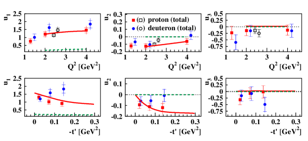
Figure 13: The $Q^{2}$ and $-t^{\prime}$ dependences of $u_{1}$, $u_{2}$, and $u_{3}$. The open symbols represent the values over the entire kinematic region. Otherwise as for Fig. 7.

Taking the amplitude without helicity flip, $U_{1\frac{1}{2}1\frac{1}{2}}$, as the dominant UPE one, Eq. (36) can be simplified as

$$u_{2}+iu_{3}=\frac{\sqrt{2}}{\mathcal{N}}U_{1\frac{1}{2}1\frac{1}{2}}U^{*}_{1\frac{1}{2}0\frac{1}{2}}\equiv\frac{\sqrt{2}}{\mathcal{N}}U_{11}U^{*}_{10}.$$ (37)

The expressions for the phase difference $\delta_{U}$ between the UPE amplitudes $U_{11}$ and $U_{10}$ follow immediately from Eq. (37):

$$\cos\delta_{U}=u_{2}/\sqrt{(u_{2})^{2}+(u_{3})^{2}},$$ (38)

$$\sin\delta_{U}=u_{3}/\sqrt{(u_{2})^{2}+(u_{3})^{2}},$$ (39)

$$\tan\delta_{U}=u_{3}/u_{2}=\frac{r^{8}_{11}+r^{8}_{1-1}}{r^{5}_{11}+r^{5}_{1-1}}.$$ (40)

The phase differences obtained for the entire kinematic region are $\delta_{U}$ = (-126 $\pm$ 12 $\pm$ 2) degrees for proton and $\delta_{U}$ = (-100 $\pm$ 61 $\pm$ 3) degrees for deuteron data.

The phase difference $\delta_{N}$ between the NPE amplitudes $T_{11}$ and $T_{00}$ can be calculated as follows DC-24 :

$$\cos\delta_{N}=\frac{2\sqrt{\epsilon}(\mathrm{Re}\{r^{5}_{10}\}-\mathrm{Im}\{r^{6}_{10}\})}{\sqrt{r^{04}_{00}(1-r^{04}_{00}+r^{1}_{1-1}-\mathrm{Im}\{r^{2}_{1-1}\})}}.$$ (41)

The phase differences obtained for the entire kinematic region are $|\delta_{N}|$ = (51 $\pm$ 5 $\pm$ 14) degrees and $|\delta_{N}|$ = (50 $\pm$ 7 $\pm$ 16) degrees for proton and deuteron data, respectively. Using polarized SDMEs, in principle also the sign of $\delta_{N}$ can be determined from the following equation:

$$\sin\delta_{N}=\frac{2\sqrt{\epsilon}(\mathrm{Re}\{r^{8}_{10}\}+\mathrm{Im}\{r^{7}_{10}\})}{\sqrt{r^{04}_{00}(1-r^{04}_{00}+r^{1}_{1-1}-\mathrm{Im}\{r^{2}_{1-1}\})}},$$ (42)

which is given in Ref. DC-24 . For the present data, the large experimental uncertainties of the polarized SDMEs make it impossible to determine the sign of $\delta_{N}$.

5.6 Longitudinal-to-transverse cross-section ratio

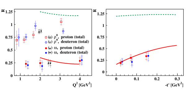
Figure 14: The $Q^{2}$ (left) and $-t^{\prime}$ (right) dependences of the longitudinal-to-transverse virtual-photon differential cross-section ratio for exclusive $\omega$ and $\rho^{0}$ electroproduction at HERMES, where the $-t^{\prime}$ bin covers the interval [0.0-0.2] GeV² for $\omega$ production and [0.0-0.4] GeV² for $\rho^{0}$ production DC-24 . The symbols that are parenthesized in the legend represent the value of $R$ in the entire kinematic region. Otherwise as for Fig. 7.

Usually, the longitudinal-to-transverse virtual-photon differential cross-section ratio

$$R=\frac{d\sigma_{L}(\gamma^{*}_{L}\to V)}{d\sigma_{T}(\gamma^{*}_{T}\to V)}$$

is experimentally determined from the measured SDME $r^{04}_{00}$ using the approximated equation DC-24

$$R\approx\frac{1}{\epsilon}\frac{r^{04}_{00}}{1-r^{04}_{00}}.$$ (43)

This relation is exact in the case of SCHC. The $Q^{2}$ dependence of $R$ for the $\omega$ meson is shown in the left panel of Fig. 14, where also for comparison the same dependence for the $\rho^{0}$ meson DC-24 is shown. For $\omega$ mesons produced in the entire kinematic region, it is found that $R$ = 0.25 $\pm$ 0.03 $\pm$ 0.07 for the proton and $R$ = 0.24 $\pm$ 0.04 $\pm$ 0.07 for the deuteron data. Compared to the case of exclusive $\rho^{0}$ production, this ratio is about four times smaller, and for the $\omega$ meson this ratio is almost independent of Q². The $-t^{\prime}$ dependence of $R$ is shown in the right panel of Fig. 14. The comparison of the proton data to the GK model calculations with and without inclusion of the pion-pole contribution demonstrates the clear need to include the pion pole. The data are well described by the model and appear to follow the $-t^{\prime}$ dependence suggested by the model when the pion-pole contribution is included. This implies that transverse and longitudinal virtual-photon cross sections have different $-t^{\prime}$ dependences. Hence the usual high-energy assumption that their ratio can be identified with the corresponding ratio of the integrated cross sections does not hold in exclusive $\omega$ electroproduction at HERMES kinematics, due to the pion-pole contribution. The GK model appears to fully account for the unnatural-parity contribution to $R$ and shows rather good agreement with the data.

5.7 The UPE-to-NPE asymmetry of the transverse cross section

The UPE-to-NPE asymmetry of the transverse differential cross section is defined as sigmat

$$P=\frac{d\sigma^{N}_{T}-d\sigma^{U}_{T}}{d\sigma^{N}_{T}+d\sigma^{U}_{T}} \equiv\frac{d\sigma^{N}_{T}/d\sigma^{U}_{T}-1}{d\sigma^{N}_{T}/d\sigma^{U}_{T}+1}$$

$$=(1+\epsilon R)(2r^{1}_{1-1}-r^{1}_{00}),$$ (44)

where $\sigma^{N}_{T}$ and $\sigma^{U}_{T}$ denote the part of the cross section due to NPE and UPE, respectively. Substituting Eq. (43) in Eq. (44) leads to the approximate relation

$$P\approx\frac{2r^{1}_{1-1}-r^{1}_{00}}{1-r^{04}_{00}}.$$ (45)

The value of $P$ obtained in the entire kinematic region is $-0.42\pm 0.06\pm 0.08$ and $-0.64\pm 0.07\pm 0.12$ for proton and deuteron, respectively. This means that a large part of the transverse cross section is due to UPE. In Fig. 15, the $Q^{2}$ and $-t^{\prime}$ dependences of the UPE-to-NPE asymmetry of the transverse differential cross section for exclusive $\omega$ production are presented. Again, the GK model calculation appears to fully account for the unnatural-parity contribution and shows very good agreement with the data both in shape and magnitude.

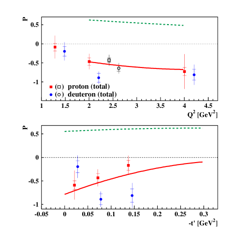
Figure 15: The $Q^{2}$ and $-t^{\prime}$ dependences of the UPE-to-NPE asymmetry $P$ of the transverse differential cross section for exclusive $\omega$ electroproduction at HERMES. The open symbols represent the values over the entire kinematic region. Otherwise as for Fig. 7.

5.8 Hierarchy of amplitudes

In order to develop a hierarchy of amplitudes, in the following a number of relations between individual helicity amplitudes is considered. The resulting hierarchy is given in Eqs. (62) and (64) below.

5.8.1 $U_{10}$ versus $U_{11}$

From Eqs. (35) and (37), the relation

$$\frac{\sqrt{2(u_{2}^{2}+u_{3}^{2})}}{u_{1}}\approx\frac{|U_{11}U^{*}_{10}|}{|U_{11}|^{2}+2\epsilon|U_{10}|^{2}}$$

$$=\frac{|U_{10}/U_{11}|}{1+2\epsilon|U_{10}/U_{11}|^{2}}$$ (46)

is obtained. Using the measured values of those SDMEs that determine $u_{1}$, $u_{2}$, and $u_{3}$, the following amplitude ratio is estimated:

$$\frac{|U_{10}|}{|U_{11}|}\approx\frac{\sqrt{2(u_{2}^{2}+u_{3}^{2})}}{u_{1}}\approx 0.2.$$ (47)

In order to reach the best possible accuracy for such estimates, the mean values of SDMEs for the proton and deuteron are used and preference will be given to quantities that do not contain polarized SDMEs, which have much less experimental accuracy than the unpolarized SDMEs. The relatively large value for the ratio $|U_{10}/U_{11}|$ is due to the large measured value of $u_{3}$. However, as this value is compatible with zero within about one standard deviation of the total uncertainty, the contribution of $u_{3}$ in Eq. (47) can be neglected, which leads to the value of $0.06$ as lower bound on $|U_{10}/U_{11}|$.

5.8.2 $T_{11}$ versus $U_{11}$

With the above considerations, it follows from Eq. (35) that the contribution of $|U_{10}/U_{11}|^{2}$ is only a few percent and hence will be neglected everywhere. Then, in particular, the relation

$$u_{1}\approx 2|U_{11}|^{2}/\mathcal{N}$$ (48)

is valid with a precision of a few percent.

Equations (7-9) show that the nucleon-helicity-flip amplitudes $T_{1\pm\frac{1}{2}1\mp\frac{1}{2}}$ ($T_{0\pm\frac{1}{2}0\mp\frac{1}{2}}$) are suppressed by a factor of about $\sqrt{-t^{\prime}}/M$ compared to the amplitude $T_{11}$ ($T_{00}$) with diagonal transitions ($\lambda^{\prime}_{N}=\lambda_{N}$). Therefore, the second-order contributions of the amplitudes $T_{\lambda\pm\frac{1}{2}\lambda\mp\frac{1}{2}}$ for any $\lambda$ will be neglected compared to any bilinear product of $T_{00}$ and $T_{11}$. In this approximation, the relation

$$\frac{2[\rm{Im}\{r^{2}_{1-1}\}-r^{2}_{1-1}]}{u_{1}}=1-\Bigl{|}\frac{T_{11}}{U_{11}}\Bigr{|}^{2}$$ (49)

follows from Eqs. (31) and (48). Substituting numerical values for the SDMEs in Eq. (49) leads to the estimate $|T_{11}/U_{11}|\approx 0.6$.

5.8.3 $T_{00}$ versus $U_{11}$

Using Eq. (48) and the expression for $r^{04}_{00}$ from Refs. Schill ; DC-24 yields

$$\frac{2r^{04}_{00}}{u_{1}}=\frac{\widetilde{\sum}[\epsilon|T_{00}|^{2}+|T_{01}|^{2}+|U_{01}|^{2}]}{|U_{11}|^{2}}.$$ (50)

Neglecting in the numerator of the right-hand side of Eq. (50) all positive terms except $|T_{00}|^{2}$, the inequality of interest is obtained:

$$\frac{2r^{04}_{00}}{u_{1}}>\frac{\epsilon|T_{00}|^{2}}{|U_{11}|^{2}}.$$ (51)

Using for the estimate $\epsilon=0.8$ and values of SDMEs from Table 1 yields the result $|T_{00}/U_{11}|<0.6$.

The same ratio can be estimated from other SDMEs. Using expressions for the SDMEs from Schill ; DC-24 , the following equations can be written:

$$\rm{Re}\{r^{5}_{10}\}-\rm{Im}\{r^{6}_{10}\}=~{}~{}~{}~{}~{}~{}~{}~{}~{}~{}~{}~{}~{}~{}~{}~{}~{}~{}~{}~{}~{}~{}~{}~{}~{}~{}~{}~{}~{}~{}~{}~{}~{}$$

$$\frac{1}{\mathcal{N}\sqrt{2}}\widetilde{\sum}{\rm Re}[T_{11}T^{*}_{00}+T_{01}T^{*}_{10}-U_{01}U^{*}_{10}],$$ (52)

$$\rm{Im}\{r^{7}_{10}\}+\rm{Re}\{r^{8}_{10}\}=~{}~{}~{}~{}~{}~{}~{}~{}~{}~{}~{}~{}~{}~{}~{}~{}~{}~{}~{}~{}~{}~{}~{}~{}~{}~{}~{}~{}~{}~{}~{}~{}~{}$$

$$\frac{1}{\mathcal{N}\sqrt{2}}\widetilde{\sum}{\rm Im}[T_{11}T^{*}_{00}+T_{10}T^{*}_{01}-U_{10}U^{*}_{01}].$$ (53)

From Eqs. (7-9), it follows that the terms $\widetilde{\sum}T_{01}T^{*}_{10}$ and $\widetilde{\sum}U_{01}U^{*}_{10}$ on the right-hand side of Eqs. (52, 53) are suppressed by a factor $(-t^{\prime})/M^{2}$ compared to $T_{11}T^{*}_{00}$ and will be neglected. The simplest consequence of Eqs. (52, 53) is the relation

$$[\rm{Re}\{r^{5}_{10}\}-\rm{Im}\{r^{6}_{10}\}]^{2}+[\rm{Im}\{r^{7}_{10}\}+\rm{Re}\{r^{8}_{10}\}]^{2}=$$

$$\frac{1}{2\mathcal{N}^{2}}|T_{11}|^{2}|T_{00}|^{2}.$$ (54)

Dividing this relation by $u_{1}^{2}/8$ and using Eq. (48), one gets the formula of interest:

$$\frac{[\rm{Re}\{r^{5}_{10}\}-\rm{Im}\{r^{6}_{10}\}]^{2}+[\rm{Im}\{r^{7}_{10}\}+\rm{Re}\{r^{8}_{10}\}]^{2}}{u^{2}_{1}/8}\approx$$

$$\frac{|T_{11}|^{2}|T_{00}|^{2}}{|U_{11}|^{4}}.~{}~{}~{}$$ (55)

Using numerical SDME values from Table 1 and $|T_{11}/U_{11}|=0.6$, the estimate $|T_{00}/U_{11}|\approx 0.5$ is obtained, which is in agreement with the previous estimate. However, as the polarized SDMEs $\rm{Im}\{r^{7}_{10}\}$ and $\rm{Re}\{r^{8}_{10}\}$ have very large uncertainties, the latter result is less reliable than the former. Omitting the contribution of the polarized SDMEs in Eq. (55) leads to the inequality

$$\frac{8[\rm{Re}\{r^{5}_{10}\}-\rm{Im}\{r^{6}_{10}\}]^{2}}{u^{2}_{1}}<\frac{|T_{11}|^{2}|T_{00}|^{2}}{|U_{11}|^{4}},$$ (56)

which provides the lower limit of $0.3$ for the same ratio $|T_{00}/U_{11}|$. This result combined with the former estimate leads to the boundaries $0.3<|T_{00}/U_{11}|<0.6$.

5.8.4 $T_{00}$ versus $T_{01}$

In order to estimate the value of $|T_{01}|$, the quantity

$$\frac{\sqrt{(r^{5}_{00})^{2}+(r^{8}_{00})^{2}}}{r^{04}_{00}}=\frac{\sqrt{2}|\widetilde{\sum}T_{01}T^{*}_{00}|}{\widetilde{\sum}[\epsilon|T_{00}|^{2}+|T_{01}|^{2}+|U_{01}|^{2}]}~{}~{}$$ (57)

can be formed. Neglecting in the denominator of the right-hand side of Eq. (57) all the terms except $\epsilon|T_{00}|^{2}$, the inequality

$$\frac{\sqrt{(r^{5}_{00})^{2}+(r^{8}_{00})^{2}}}{r^{04}_{00}}<\frac{\sqrt{2}|\widetilde{\sum}T_{01}T^{*}_{00}|}{\epsilon|T_{00}|^{2}}$$ (58)

is obtained. The sum in the numerator of the right-hand side of Eq. (58) is

$$\widetilde{\sum}T_{01}T^{*}_{00}=T_{0\frac{1}{2}1\frac{1}{2}}T^{*}_{0\frac{1}{2}0\frac{1}{2}}+T_{0-\frac{1}{2}1\frac{1}{2}}T^{*}_{0-\frac{1}{2}0\frac{1}{2}}$$ (59)

according to Eq. (11). If the first product on the right-hand side of Eq. (59) dominates, then inequality (58) becomes simpler:

$$\frac{\sqrt{(r^{5}_{00})^{2}+(r^{8}_{00})^{2}}}{r^{04}_{00}}<\frac{\sqrt{2}}{\epsilon}\frac{|T_{01}|}{|T_{00}|}.$$ (60)

Numerically, this yields the estimate $|T_{01}/T_{00}|\simeq 0.3$. The dominant contribution to this number comes from the polarized SDME $r^{8}_{00}$ that is compatible with zero within about one standard deviation of the total uncertainty. Retaining only the contribution of the unpolarized SDME $r^{5}_{00}$ in Eq. (60) gives the following result: $|T_{01}/T_{00}|>0.1$. The experimental accuracy of the presented data is not sufficient to provide a reliable estimate for the upper bound to the ratio $|T_{01}/T_{00}|$. As shown in Appendix A, the upper limits for

$$\mathcal{A}\equiv\frac{\widetilde{\sum}(|T_{01}|^{2}+|U_{01}|^{2})}{|T_{00}|^{2}}$$ (61)

are $1.3\pm 0.7$ for the proton and $1.1\pm 1.2$ for the deuteron. In the below consideration the estimate based on Eq. (60), namely $|T_{01}/T_{00}|\simeq 0.3$, is assumed to be realistic.

The numerator in the definition of $r^{1}_{00}$ is $\widetilde{\sum}[|U_{01}|^{2}-|T_{01}|^{2}]$. The values of $r^{1}_{00}$ are compatible with zero within two standard deviations of the total experimental uncertainty, hence $|U_{01}|$ cannot be much larger than $|T_{01}|$.
Considering the SDME combinations ($r^{5}_{11}-r^{5}_{1-1}$) and ($\rm{Im}\{r^{8}_{1-1}\}-r^{8}_{11}$), which are proportional to the real and imaginary parts of $\widetilde{\sum}T_{10}(T_{11}-T_{1-1})^{*}$, respectively, it is possible in principle to estimate the value of $|T_{10}|$. Since these combinations are compatible with zero within one standard deviation of the total uncertainty, it can be concluded that $|T_{10}|$ is negligibly small compared to the large amplitude moduli $|U_{11}|$, $|T_{11}|$, and $|T_{00}|$.

5.8.5 Resulting hierarchy of amplitudes

As a result, the following hierarchy is obtained:

$$|U_{11}|^{2}>|T_{00}|^{2}\sim|T_{11}|^{2}$$

$$\gg\ |U_{10}|^{2}\sim|T_{01}|^{2}\sim|U_{01}|^{2}$$

$$\gg\ |T_{10}|^{2},|T_{1-1}|^{2},|U_{1-1}|^{2},$$ (62)

where negligibly small amplitudes are neglected.

However, there exists a possible alternative for the hierarchy presented on the second line of Eq. (62), if the helicity-flip amplitudes $T_{0-\frac{1}{2}1\frac{1}{2}}$ and $U_{0-\frac{1}{2}1\frac{1}{2}}$ are of the same order of magnitude as the helicity-conserving amplitudes $T_{00}$ and $T_{11}$. Indeed, the sum $\widetilde{\sum}T_{01}T^{*}_{00}$ in Eq. (58) is the sum of two products, $T_{0\frac{1}{2}1\frac{1}{2}}T^{*}_{0\frac{1}{2}0\frac{1}{2}}$ and $T_{0-\frac{1}{2}1\frac{1}{2}}T^{*}_{0-\frac{1}{2}0\frac{1}{2}}$, according to Eq. (59). In order to obtain Eq. (60) from Eq. (58), the dominance of the first product was assumed. If instead the second product is assumed to be dominant, Eq. (60) has to be replaced by

$$\frac{\sqrt{(r^{5}_{00})^{2}+(r^{8}_{00})^{2}}}{r^{04}_{00}} \leq\frac{\sqrt{2}}{\epsilon}\frac{|T_{0-\frac{1}{2}1\frac{1}{2}}T^{*}_{0-\frac{1}{2}0\frac{1}{2}}|}{|T_{00}|^{2}}$$

$$=\frac{\sqrt{2}}{\epsilon}\frac{|T_{0-\frac{1}{2}1\frac{1}{2}}|}{|T_{00}|}\frac{|T_{0-\frac{1}{2}0\frac{1}{2}}|}{|T_{00}|}.$$ (63)

The nucleon-helicity-flip amplitude $T_{0-\frac{1}{2}0\frac{1}{2}}$ is smaller than the helicity-conserving amplitude $T_{00}\equiv T_{0\frac{1}{2}0\frac{1}{2}}$ by a factor of about $\sqrt{-t^{\prime}}/M\approx 0.3$ (see Eq. (9)). Substituting this factor for $|T_{0-\frac{1}{2}0\frac{1}{2}}/T_{00}|$, using $\epsilon=0.8$ and the measured SDME values, the final estimate $|T_{0-\frac{1}{2}1\frac{1}{2}}|\simeq|T_{00}|$ is obtained. This result shows that the nucleon-helicity-flip amplitude $T_{0-\frac{1}{2}1\frac{1}{2}}$ could be of the same order of magnitude as $T_{00}$, while the values of $T_{01}$ and $U_{01}$ could be as given in the previous estimates.

As the SDME $r^{1}_{00}$, which is proportional to $\widetilde{\sum}[|U_{01}|^{2}-|T_{01}|^{2}]$, was measured to be compatible with zero, the value of $|U_{0-\frac{1}{2}1\frac{1}{2}}|$ should be about the same as that of $|T_{0-\frac{1}{2}1\frac{1}{2}}|$. Then, the values of $|T_{0-\frac{1}{2}1\frac{1}{2}}|$, $|U_{0-\frac{1}{2}1\frac{1}{2}}|$, and $|T_{00}|$ are of the same order of magnitude, so that the hierarchy of amplitudes becomes

$$|U_{11}|^{2} >|T_{00}|^{2}\sim|T_{11}|^{2}\sim|T_{0-\frac{1}{2}1\frac{1}{2}}|^{2}\sim|U_{0-\frac{1}{2}1\frac{1}{2}}|^{2}$$

$$\gg|U_{10}|^{2}\sim|T_{01}|^{2}\sim|U_{01}|^{2}$$

$$\gg|T_{10}|^{2},|T_{1-1}|^{2},|U_{1-1}|^{2},$$ (64)

where again negligibly small amplitudes are neglected. Note that the usually used Eq. (43) for $R$ is not applicable in this case. The estimation performed in Appendix A shows that the accuracy of the presented data is not sufficient to decide between hierarchies (62) and (64). The best way to get information on the amplitudes $T_{0-\frac{1}{2}1\frac{1}{2}}$ and $U_{0-\frac{1}{2}1\frac{1}{2}}$ is to study electroproduction of $\omega$ mesons on transversely polarized protons, where these amplitudes contribute linearly to the angular distribution.

6 Summary

Exclusive $\omega$ electroproduction is studied at HERMES using a longitudinally polarized lepton beam and unpolarized hydrogen and deuterium targets in the kinematic region $Q^{2}>1.0$ GeV², $3.0$ GeV $<W<6.3$ GeV, and $-t^{\prime}<0.2$ GeV². The average kinematic values are $\langle Q^{2}\rangle=2.42$ GeV², $\langle W\rangle=4.8$ GeV, and $\langle-t^{\prime}\rangle=0.080$ GeV². Using an unbinned maximum likelihood method, 15 unpolarized and, for the first time, 8 polarized spin density matrix elements are extracted. The kinematic dependences of all 23 SDMEs are presented for proton and deuteron data. No significant differences between proton and deuteron results are seen.

The SDMEs are presented in five classes corresponding to different helicity transitions between the virtual photon and the $\omega$ meson. While the values of class-A and B SDMEs agree with the hypothesis of $s$-channel helicity conservation, the class-C SDME $r^{5}_{00}$ indicates a violation of this hypothesis. The values of those class-D SDMEs that correspond to the transition $\gamma^{*}_{L}\to\omega_{T}$ also indicate a small violation of the hypothesis of $s$-channel helicity conservation.

Using the SDMEs $r_{1-1}^{1}$ and $\mathrm{Im}\{r_{1-1}^{2}\}$, it is shown that for exclusive $\omega$-meson production the amplitude of the UPE transition $\gamma^{*}_{T}\to\omega_{T}$ is larger than the NPE amplitude for the same transition, i.e., $|U_{11}|^{2}>|T_{11}|^{2}$. The importance of UPE transitions is also shown by a combination of SDMEs denoted $u_{1}$. This suggests that at HERMES energies in exclusive $\omega$ electroproduction the quark-exchange mechanism, or $\pi^{0}$, $a_{1}$… exchanges in Regge phenomenology, plays a significant role.

The phase shift between those UPE amplitudes that describe transverse $\omega$ production by transverse and longitudinal virtual photons, $U_{11}$ for $\gamma^{*}_{T}\to\omega_{T}$ and $U_{10}$ for $\gamma^{*}_{L}\to\omega_{T}$, respectively, as well as the magnitude of the phase difference between the NPE amplitudes $T_{11}$ and $T_{00}$ is determined for the first time.

The ratio $R$ between the differential longitudinal and transverse virtual-photon cross-sections is determined to be $R$ = 0.25 $\pm$ 0.03 $\pm$ 0.07 for the $\omega$ meson, which is about four times smaller than in the case of the $\rho^{0}$ meson. In contrast to the case of the $\rho^{0}$ meson, $R$ shows only a weak dependence on $Q^{2}$ for the $\omega$ meson.

The UPE-to-NPE asymmetry of the transverse virtual-photon cross section is determined to be $P=-0.42\pm 0.06\pm 0.08$ and $P=-0.64\pm 0.07\pm 0.12$ for the proton and deuteron data, respectively.

From the extracted SDMEs, two slightly different hierarchies of helicity amplitudes can be derived, which remain indistinguishable for the given experimental accuracy of the presented data. Both hierarchies consistently mean that the UPE amplitude describing the $\gamma^{*}_{T}\rightarrow\omega_{T}$ transition dominates over the two NPE amplitudes describing the $\gamma^{*}_{L}\rightarrow\omega_{L}$ and $\gamma^{*}_{T}\rightarrow\omega_{T}$ transitions, with the latter two being of similar magnitude.

Good agreement between the presented proton data and results of a pQCD-inspired phenomenological model is found only when including pion-pole contributions, which are of unnatural parity. The distinct $-t^{\prime}$ dependence of the pion-pole contribution leads to a $-t^{\prime}$ dependence of $R$. This invalidates for exclusive $\omega$ production at HERMES energies the common high-energy assumption of identifying $R$ with the ratio of the integrated longitudinal and transverse cross sections.

Appendix A Estimate of $T_{0-\frac{1}{2}1\frac{1}{2}}$ and $U_{0-\frac{1}{2}1\frac{1}{2}}$ values

The normalization factor $\mathcal{N}$ is given by (see, e.g., Schill ; DC-24 )

$$\mathcal{N}=\mathcal{N}_{T}+\epsilon\mathcal{N}_{L},$$ (65)

with

$$\mathcal{N}_{T}=\widetilde{\sum}( |T_{11}|^{2}+|T_{01}|^{2}+|T_{-11}|^{2}$$

$$+|U_{11}|^{2}+|U_{01}|^{2}+|U_{-11}|^{2}),$$ (66)

$$\mathcal{N}_{L}=\widetilde{\sum}( |T_{00}|^{2}+2|T_{10}|^{2}+2|U_{10}|^{2}).$$ (67)

Using Eqs. (65-67) and the expression defining $r^{04}_{00}$ Schill ; DC-24 ,

$$r^{04}_{00}=\frac{1}{\mathcal{N}}\widetilde{\sum}(\epsilon|T_{00}|^{2}+|T_{01}|^{2}+|U_{01}|^{2}),$$ (68)

the exact relation

$$1-r^{04}_{00}=\frac{1}{\mathcal{N}}\widetilde{\sum}[ |T_{11}|^{2}+|U_{11}|^{2}+|T_{1-1}|^{2}+|U_{1-1}|^{2}$$

$$+2\epsilon(|T_{10}|^{2}+|U_{10}|^{2})]$$ (69)

is obtained. Neglecting, as usual, $\widetilde{\sum}[|T_{1-1}|^{2}+|U_{1-1}|^{2}+|T_{10}|^{2}+|U_{10}|^{2}]$ in this expression, we get the approximate relation

$$1-r^{04}_{00}\approx\frac{1}{\mathcal{N}}\widetilde{\sum}(|T_{11}|^{2}+|U_{11}|^{2}).$$ (70)

Neglecting also the small nucleon-helicity-flip amplitudes $T_{1-\frac{1}{2}1\frac{1}{2}}$ and $U_{1-\frac{1}{2}1\frac{1}{2}}$ in Eq. (30) and then subtracting it from Eq. (70), the relation

$$1-r^{04}_{00}+r^{1}_{1-1}-\rm{Im}\{r^{2}_{1-1}\}\approx\frac{2}{\mathcal{N}}|T_{11}|^{2}$$ (71)

is obtained. After neglecting in Eq. (68) only the nucleon-helicity-flip amplitude $T_{0-\frac{1}{2}0\frac{1}{2}}$, it can be rewritten as

$$r^{04}_{00}\approx\frac{1}{\mathcal{N}}\left[\epsilon|T_{00}|^{2}+\widetilde{\sum}(|T_{01}|^{2}+|U_{01}|^{2})\right].$$ (72)

Multiplying this equation by Eq. (71) and dividing it by Eq. (54) with a factor of four, the equation of interest reads

$$\epsilon+\mathcal{A}\approx~{}~{}~{}~{}~{}~{}~{}~{}~{}~{}~{}~{}~{}~{}~{}~{}~{}~{}~{}~{}~{}~{}~{}~{}~{}~{}~{}~{}~{}~{}~{}~{}~{}~{}~{}~{}~{}~{}~{}~{}~{}~{}~{}~{}~{}~{}~{}~{}~{}~{}~{}~{}~{}~{}~{}~{}~{}~{}~{}$$

$$\frac{r^{04}_{00}(1-r^{04}_{00}+r^{1}_{1-1}-\rm{Im}\{r^{2}_{1-1}\})/4}{[\rm{Re}\{r^{5}_{10}\}-\rm{Im}\{r^{6}_{10}\}]^{2}+[\rm{Im}\{r^{7}_{10}\}+\rm{Re}\{r^{8}_{10}\}]^{2}},~{}~{}~{}~{}$$ (73)

where the quantity $\mathcal{A}$ is defined in Eq. (61). The value of $\mathcal{A}$ is close to zero, if $|T_{0-\frac{1}{2}1\frac{1}{2}}|^{2}$ and $|U_{0-\frac{1}{2}1\frac{1}{2}}|^{2}$ are much smaller than $|T_{00}|^{2}$, and it should be of the order of one if they are comparable to $|T_{00}|^{2}$. Since the uncertainties of the polarized SDMEs $\rm{Im}\{r^{7}_{10}\}$ and $\rm{Re}\{r^{8}_{10}\}$ are large, the use of Eq. (73) for the present data is not very successful. Indeed, using for numerical calculations $\epsilon=0.8$ and the values for the SDMEs in Eq. (73) from Table 1 we get $\mathcal{A}=-0.56\pm 0.20$ and $\mathcal{A}=0.50\pm 1.8$ for the proton and deuteron data, respectively. In contrast, in $\rho^{0}$-meson production, the corresponding values of $\mathcal{A}$ DC-24 , $-0.031\pm 0.084$ and $-0.064\pm 0.068$, exclude practically the possibility that the amplitudes $T_{0-\frac{1}{2}1\frac{1}{2}}$ and $U_{0-\frac{1}{2}1\frac{1}{2}}$ are comparable to the dominant amplitudes $U_{11}$, $T_{00}$ and $T_{11}$.
If the contribution of $[\rm{Im}\{r^{7}_{10}\}+\rm{Re}\{r^{8}_{10}\}]$ in the denominator of the right-hand side of Eq. (73) is neglected, the useful inequality

$$\mathcal{A}\leq\frac{r^{04}_{00}(1-r^{04}_{00}+r^{1}_{1-1}-\rm{Im}\{r^{2}_{1-1}\})}{4[\rm{Re}\{r^{5}_{10}\}-\rm{Im}\{r^{6}_{10}\}]^{2}}-\epsilon$$ (74)

can be obtained. The numerical estimates $\mathcal{A}\leq 1.3\pm 0.7$ and $\mathcal{A}\leq 1.1\pm 1.2$ for the proton and deuteron data, respectively, show that the possibility for the values of $|T_{0-\frac{1}{2}1\frac{1}{2}}|^{2}$ and $|U_{0-\frac{1}{2}1\frac{1}{2}}|^{2}$ to be of the same order of magnitude as $|T_{00}|^{2}$ is not excluded by the presented results on $\omega$ SDMEs. For comparison, when applying Eq. (74) to the results on proton and deuteron data in exclusive $\rho^{0}$-meson production DC-24 , one obtains $\mathcal{A}\leq 0.22\pm 0.09$ and $\mathcal{A}\leq 0.28\pm 0.09$, respectively. This shows that in this case the probability for the amplitudes $T_{0-\frac{1}{2}1\frac{1}{2}}$ and $U_{0-\frac{1}{2}1\frac{1}{2}}$ to be of the same order of magnitude as $T_{00}$ is small.

Appendix B SDMEs for proton and deuteron

Table 1: The 23 unpolarized and polarized $\omega$ SDMEs from the proton and deuteron data. The first uncertainty is statistical, the second systematic.

element	proton	deuteron
$r^{04}_{00}$	0.168 $\pm$ 0.018 $\pm$ 0.036	0.160 $\pm$ 0.024 $\pm$ 0.038
$r^{1}_{1-1}$	-0.175 $\pm$ 0.029 $\pm$ 0.039	-0.215 $\pm$ 0.036 $\pm$ 0.047
Im $r^{2}_{1-1}$	0.171 $\pm$ 0.029 $\pm$ 0.023	0.248 $\pm$ 0.037 $\pm$ 0.039
Re $r^{5}_{10}$	0.037 $\pm$ 0.009 $\pm$ 0.012	0.045 $\pm$ 0.010 $\pm$ 0.014
Im $r^{6}_{10}$	-0.061 $\pm$ 0.008 $\pm$ 0.012	-0.043 $\pm$ 0.010 $\pm$ 0.009
Im $r^{7}_{10}$	0.109 $\pm$ 0.075 $\pm$ 0.021	0.021 $\pm$ 0.087 $\pm$ 0.004
Re $r^{8}_{10}$	0.169 $\pm$ 0.075 $\pm$ 0.035	-0.083 $\pm$ 0.083 $\pm$ 0.017
Re $r^{04}_{10}$	-0.010 $\pm$ 0.012 $\pm$ 0.002	0.020 $\pm$ 0.014 $\pm$ 0.005
Re $r^{1}_{10}$	-0.014 $\pm$ 0.019 $\pm$ 0.005	0.016 $\pm$ 0.022 $\pm$ 0.009
Im $r^{2}_{10}$	0.039 $\pm$ 0.018 $\pm$ 0.007	-0.003 $\pm$ 0.023 $\pm$ 0.002
$r^{5}_{00}$	0.042 $\pm$ 0.015 $\pm$ 0.012	0.036 $\pm$ 0.019 $\pm$ 0.014
$r^{1}_{00}$	0.006 $\pm$ 0.029 $\pm$ 0.008	0.107 $\pm$ 0.036 $\pm$ 0.023
Im $r^{3}_{10}$	0.059 $\pm$ 0.047 $\pm$ 0.012	0.038 $\pm$ 0.056 $\pm$ 0.008
$r^{8}_{00}$	-0.142 $\pm$ 0.110 $\pm$ 0.029	-0.017 $\pm$ 0.131 $\pm$ 0.004
$r^{5}_{11}$	-0.059 $\pm$ 0.012 $\pm$ 0.022	-0.025 $\pm$ 0.015 $\pm$ 0.015
$r^{5}_{1-1}$	-0.043 $\pm$ 0.014 $\pm$ 0.006	-0.021 $\pm$ 0.018 $\pm$ 0.001
Im $r^{6}_{1-1}$	0.036 $\pm$ 0.014 $\pm$ 0.008	0.056 $\pm$ 0.019 $\pm$ 0.013
Im $r^{7}_{1-1}$	-0.092 $\pm$ 0.117 $\pm$ 0.018	0.113 $\pm$ 0.135 $\pm$ 0.028
$r^{8}_{11}$	-0.079 $\pm$ 0.089 $\pm$ 0.017	-0.097 $\pm$ 0.103 $\pm$ 0.020
Im $r^{8}_{1-1}$	-0.060 $\pm$ 0.110 $\pm$ 0.012	-0.150 $\pm$ 0.125 $\pm$ 0.034
$r^{04}_{1-1}$	-0.004 $\pm$ 0.018 $\pm$ 0.004	0.060 $\pm$ 0.023 $\pm$ 0.016
$r^{1}_{11}$	0.014 $\pm$ 0.024 $\pm$ 0.004	-0.037 $\pm$ 0.030 $\pm$ 0.007
$r^{3}_{1-1}$	0.023 $\pm$ 0.076 $\pm$ 0.010	-0.122 $\pm$ 0.089 $\pm$ 0.025

Table 2: The 23 unpolarized and polarized $\omega$ SDMEs for the proton data in $Q^{2}$ intervals: $1.00-1.57-2.55-10.00$ GeV². The first uncertainty is statistical, the second systematic.

element	$\langle$Q2$\rangle$ = 1.28 GeV2	$\langle$Q2$\rangle$ = 2.00 GeV2	$\langle$Q2$\rangle$ = 4.00 GeV2
$r^{04}_{00}$	0.164 $\pm$ 0.034 $\pm$ 0.022	0.166 $\pm$ 0.030 $\pm$ 0.044	0.179 $\pm$ 0.031 $\pm$ 0.036
$r^{1}_{1-1}$	-0.032 $\pm$ 0.050 $\pm$ 0.032	-0.175 $\pm$ 0.049 $\pm$ 0.037	-0.314 $\pm$ 0.053 $\pm$ 0.090
Im $r^{2}_{1-1}$	0.172 $\pm$ 0.048 $\pm$ 0.027	0.133 $\pm$ 0.050 $\pm$ 0.043	0.163 $\pm$ 0.057 $\pm$ 0.029
Re $r^{5}_{10}$	0.038 $\pm$ 0.016 $\pm$ 0.018	0.022 $\pm$ 0.015 $\pm$ 0.010	0.053 $\pm$ 0.015 $\pm$ 0.022
Im $r^{6}_{10}$	-0.062 $\pm$ 0.015 $\pm$ 0.012	-0.069 $\pm$ 0.012 $\pm$ 0.014	-0.046 $\pm$ 0.014 $\pm$ 0.013
Im $r^{7}_{10}$	0.163 $\pm$ 0.139 $\pm$ 0.030	-0.006 $\pm$ 0.125 $\pm$ 0.009	0.170 $\pm$ 0.128 $\pm$ 0.042
Re $r^{8}_{10}$	0.088 $\pm$ 0.143 $\pm$ 0.021	0.078 $\pm$ 0.137 $\pm$ 0.028	0.280 $\pm$ 0.119 $\pm$ 0.067
Re $r^{04}_{10}$	0.005 $\pm$ 0.021 $\pm$ 0.004	-0.060 $\pm$ 0.020 $\pm$ 0.011	0.016 $\pm$ 0.019 $\pm$ 0.022
Re $r^{1}_{10}$	-0.005 $\pm$ 0.032 $\pm$ 0.013	-0.090 $\pm$ 0.031 $\pm$ 0.012	0.073 $\pm$ 0.034 $\pm$ 0.016
Im $r^{2}_{10}$	0.012 $\pm$ 0.030 $\pm$ 0.012	0.042 $\pm$ 0.030 $\pm$ 0.003	0.036 $\pm$ 0.034 $\pm$ 0.016
$r^{5}_{00}$	0.031 $\pm$ 0.029 $\pm$ 0.001	0.029 $\pm$ 0.025 $\pm$ 0.012	0.068 $\pm$ 0.027 $\pm$ 0.016
$r^{1}_{00}$	0.009 $\pm$ 0.049 $\pm$ 0.011	0.039 $\pm$ 0.049 $\pm$ 0.013	-0.032 $\pm$ 0.053 $\pm$ 0.015
Im $r^{3}_{10}$	0.044 $\pm$ 0.096 $\pm$ 0.008	0.047 $\pm$ 0.076 $\pm$ 0.009	0.073 $\pm$ 0.076 $\pm$ 0.018
$r^{8}_{00}$	-0.147 $\pm$ 0.210 $\pm$ 0.039	0.035 $\pm$ 0.196 $\pm$ 0.026	-0.197 $\pm$ 0.171 $\pm$ 0.045
$r^{5}_{11}$	-0.074 $\pm$ 0.020 $\pm$ 0.021	-0.050 $\pm$ 0.020 $\pm$ 0.012	-0.070 $\pm$ 0.021 $\pm$ 0.029
$r^{5}_{1-1}$	-0.047 $\pm$ 0.024 $\pm$ 0.007	-0.078 $\pm$ 0.025 $\pm$ 0.021	0.008 $\pm$ 0.025 $\pm$ 0.009
Im $r^{6}_{1-1}$	0.070 $\pm$ 0.025 $\pm$ 0.013	-0.015 $\pm$ 0.024 $\pm$ 0.017	0.043 $\pm$ 0.026 $\pm$ 0.026
Im $r^{7}_{1-1}$	-0.326 $\pm$ 0.223 $\pm$ 0.058	-0.161 $\pm$ 0.198 $\pm$ 0.030	0.046 $\pm$ 0.204 $\pm$ 0.023
$r^{8}_{11}$	0.276 $\pm$ 0.171 $\pm$ 0.049	-0.120 $\pm$ 0.155 $\pm$ 0.021	-0.312 $\pm$ 0.144 $\pm$ 0.080
Im $r^{8}_{1-1}$	-0.507 $\pm$ 0.212 $\pm$ 0.093	-0.026 $\pm$ 0.188 $\pm$ 0.005	0.185 $\pm$ 0.178 $\pm$ 0.063
$r^{04}_{1-1}$	-0.004 $\pm$ 0.032 $\pm$ 0.000	-0.023 $\pm$ 0.031 $\pm$ 0.003	0.008 $\pm$ 0.031 $\pm$ 0.014
$r^{1}_{11}$	0.063 $\pm$ 0.040 $\pm$ 0.015	-0.037 $\pm$ 0.041 $\pm$ 0.012	0.003 $\pm$ 0.044 $\pm$ 0.012
$r^{3}_{1-1}$	0.074 $\pm$ 0.153 $\pm$ 0.013	-0.110 $\pm$ 0.131 $\pm$ 0.021	0.088 $\pm$ 0.124 $\pm$ 0.024

Table 3: The 23 unpolarized and polarized $\omega$ SDMEs for the proton data in $-t^{\prime}$ intervals: $0.000-0.044-0.105-0.200$ GeV². The first uncertainty is statistical, the second systematic.

element	$\langle-t^{\prime}\rangle$ = 0.021 GeV2	$\langle-t^{\prime}\rangle$ = 0.072 GeV2	$\langle-t^{\prime}\rangle$ = 0.147 GeV2
$r^{04}_{00}$	0.136 $\pm$ 0.027 $\pm$ 0.036	0.197 $\pm$ 0.032 $\pm$ 0.027	0.212 $\pm$ 0.036 $\pm$ 0.032
$r^{1}_{1-1}$	-0.239 $\pm$ 0.043 $\pm$ 0.023	-0.141 $\pm$ 0.048 $\pm$ 0.043	-0.120 $\pm$ 0.060 $\pm$ 0.048
Im $r^{2}_{1-1}$	0.220 $\pm$ 0.045 $\pm$ 0.033	0.138 $\pm$ 0.050 $\pm$ 0.015	0.111 $\pm$ 0.057 $\pm$ 0.012
Re $r^{5}_{10}$	0.015 $\pm$ 0.013 $\pm$ 0.008	0.032 $\pm$ 0.015 $\pm$ 0.010	0.081 $\pm$ 0.018 $\pm$ 0.025
Im $r^{6}_{10}$	-0.051 $\pm$ 0.012 $\pm$ 0.012	-0.077 $\pm$ 0.013 $\pm$ 0.013	-0.058 $\pm$ 0.015 $\pm$ 0.018
Im $r^{7}_{10}$	-0.143 $\pm$ 0.121 $\pm$ 0.037	0.340 $\pm$ 0.123 $\pm$ 0.071	0.277 $\pm$ 0.146 $\pm$ 0.073
Re $r^{8}_{10}$	0.151 $\pm$ 0.125 $\pm$ 0.039	0.232 $\pm$ 0.127 $\pm$ 0.044	0.151 $\pm$ 0.136 $\pm$ 0.039
Re $r^{04}_{10}$	-0.022 $\pm$ 0.018 $\pm$ 0.004	0.010 $\pm$ 0.020 $\pm$ 0.006	0.006 $\pm$ 0.023 $\pm$ 0.002
Re $r^{1}_{10}$	-0.020 $\pm$ 0.030 $\pm$ 0.007	-0.013 $\pm$ 0.032 $\pm$ 0.001	-0.029 $\pm$ 0.035 $\pm$ 0.011
Im $r^{2}_{10}$	0.017 $\pm$ 0.029 $\pm$ 0.008	-0.003 $\pm$ 0.029 $\pm$ 0.005	0.125 $\pm$ 0.033 $\pm$ 0.023
$r^{5}_{00}$	-0.016 $\pm$ 0.023 $\pm$ 0.029	0.059 $\pm$ 0.027 $\pm$ 0.011	0.100 $\pm$ 0.031 $\pm$ 0.012
$r^{1}_{00}$	0.032 $\pm$ 0.047 $\pm$ 0.033	0.067 $\pm$ 0.050 $\pm$ 0.024	-0.106 $\pm$ 0.053 $\pm$ 0.067
Im $r^{3}_{10}$	0.063 $\pm$ 0.073 $\pm$ 0.010	0.076 $\pm$ 0.082 $\pm$ 0.018	0.121 $\pm$ 0.090 $\pm$ 0.036
$r^{8}_{00}$	0.155 $\pm$ 0.179 $\pm$ 0.033	-0.138 $\pm$ 0.197 $\pm$ 0.026	-0.442 $\pm$ 0.191 $\pm$ 0.115
$r^{5}_{11}$	-0.059 $\pm$ 0.018 $\pm$ 0.012	-0.051 $\pm$ 0.020 $\pm$ 0.015	-0.068 $\pm$ 0.024 $\pm$ 0.048
$r^{5}_{1-1}$	-0.034 $\pm$ 0.022 $\pm$ 0.002	-0.060 $\pm$ 0.024 $\pm$ 0.007	-0.052 $\pm$ 0.030 $\pm$ 0.011
Im $r^{6}_{1-1}$	0.010 $\pm$ 0.022 $\pm$ 0.000	0.090 $\pm$ 0.024 $\pm$ 0.020	0.020 $\pm$ 0.028 $\pm$ 0.009
Im $r^{7}_{1-1}$	-0.027 $\pm$ 0.176 $\pm$ 0.004	0.244 $\pm$ 0.197 $\pm$ 0.046	-0.601 $\pm$ 0.233 $\pm$ 0.165
$r^{8}_{11}$	-0.136 $\pm$ 0.145 $\pm$ 0.023	-0.155 $\pm$ 0.150 $\pm$ 0.029	0.038 $\pm$ 0.169 $\pm$ 0.010
Im $r^{8}_{1-1}$	-0.182 $\pm$ 0.181 $\pm$ 0.046	0.085 $\pm$ 0.180 $\pm$ 0.017	-0.055 $\pm$ 0.210 $\pm$ 0.025
$r^{04}_{1-1}$	-0.006 $\pm$ 0.029 $\pm$ 0.003	-0.007 $\pm$ 0.030 $\pm$ 0.006	-0.023 $\pm$ 0.036 $\pm$ 0.008
$r^{1}_{11}$	0.009 $\pm$ 0.037 $\pm$ 0.005	0.023 $\pm$ 0.040 $\pm$ 0.006	0.033 $\pm$ 0.047 $\pm$ 0.029
$r^{3}_{1-1}$	-0.016 $\pm$ 0.111 $\pm$ 0.006	0.160 $\pm$ 0.134 $\pm$ 0.036	-0.154 $\pm$ 0.156 $\pm$ 0.054

Table 4: The 23 unpolarized and polarized $\omega$ SDMEs for the deuteron data in $Q^{2}$ intervals: $1.00-1.57-2.55-10.00$ GeV². The first uncertainty is statistical, the second systematic.

element	$\langle$Q2$\rangle$ = 1.28 GeV2	$\langle$Q2$\rangle$ = 2.00 GeV2	$\langle$Q2$\rangle$ = 4.00 GeV2
$r^{04}_{00}$	0.148 $\pm$ 0.043 $\pm$ 0.025	0.132 $\pm$ 0.041 $\pm$ 0.053	0.186 $\pm$ 0.040 $\pm$ 0.034
$r^{1}_{1-1}$	-0.045 $\pm$ 0.063 $\pm$ 0.030	-0.347 $\pm$ 0.058 $\pm$ 0.075	-0.258 $\pm$ 0.072 $\pm$ 0.070
Im $r^{2}_{1-1}$	0.232 $\pm$ 0.063 $\pm$ 0.045	0.216 $\pm$ 0.065 $\pm$ 0.063	0.313 $\pm$ 0.073 $\pm$ 0.056
Re $r^{5}_{10}$	0.059 $\pm$ 0.020 $\pm$ 0.021	0.056 $\pm$ 0.017 $\pm$ 0.015	0.025 $\pm$ 0.020 $\pm$ 0.014
Im $r^{6}_{10}$	-0.034 $\pm$ 0.018 $\pm$ 0.006	-0.039 $\pm$ 0.016 $\pm$ 0.009	-0.055 $\pm$ 0.021 $\pm$ 0.015
Im $r^{7}_{10}$	-0.174 $\pm$ 0.160 $\pm$ 0.032	0.225 $\pm$ 0.150 $\pm$ 0.044	-0.068 $\pm$ 0.156 $\pm$ 0.015
Re $r^{8}_{10}$	-0.026 $\pm$ 0.154 $\pm$ 0.005	-0.197 $\pm$ 0.148 $\pm$ 0.039	0.020 $\pm$ 0.140 $\pm$ 0.004
Re $r^{04}_{10}$	-0.004 $\pm$ 0.027 $\pm$ 0.007	0.020 $\pm$ 0.024 $\pm$ 0.011	0.040 $\pm$ 0.025 $\pm$ 0.012
Re $r^{1}_{10}$	-0.039 $\pm$ 0.037 $\pm$ 0.019	0.052 $\pm$ 0.037 $\pm$ 0.015	0.025 $\pm$ 0.046 $\pm$ 0.008
Im $r^{2}_{10}$	0.014 $\pm$ 0.037 $\pm$ 0.013	0.003 $\pm$ 0.036 $\pm$ 0.012	-0.028 $\pm$ 0.049 $\pm$ 0.004
$r^{5}_{00}$	0.074 $\pm$ 0.033 $\pm$ 0.007	0.050 $\pm$ 0.032 $\pm$ 0.012	-0.006 $\pm$ 0.035 $\pm$ 0.031
$r^{1}_{00}$	0.079 $\pm$ 0.061 $\pm$ 0.028	0.077 $\pm$ 0.059 $\pm$ 0.012	0.143 $\pm$ 0.073 $\pm$ 0.048
Im $r^{3}_{10}$	0.124 $\pm$ 0.107 $\pm$ 0.031	0.009 $\pm$ 0.095 $\pm$ 0.002	0.016 $\pm$ 0.096 $\pm$ 0.004
$r^{8}_{00}$	0.186 $\pm$ 0.248 $\pm$ 0.041	-0.024 $\pm$ 0.242 $\pm$ 0.005	-0.088 $\pm$ 0.211 $\pm$ 0.019
$r^{5}_{11}$	-0.027 $\pm$ 0.026 $\pm$ 0.013	-0.054 $\pm$ 0.025 $\pm$ 0.018	-0.001 $\pm$ 0.030 $\pm$ 0.011
$r^{5}_{1-1}$	-0.040 $\pm$ 0.031 $\pm$ 0.005	-0.049 $\pm$ 0.031 $\pm$ 0.010	0.021 $\pm$ 0.036 $\pm$ 0.009
Im $r^{6}_{1-1}$	0.062 $\pm$ 0.031 $\pm$ 0.016	0.050 $\pm$ 0.032 $\pm$ 0.004	0.057 $\pm$ 0.035 $\pm$ 0.021
Im $r^{7}_{1-1}$	0.399 $\pm$ 0.250 $\pm$ 0.079	-0.053 $\pm$ 0.236 $\pm$ 0.011	-0.003 $\pm$ 0.234 $\pm$ 0.001
$r^{8}_{11}$	-0.332 $\pm$ 0.193 $\pm$ 0.059	-0.103 $\pm$ 0.184 $\pm$ 0.020	-0.022 $\pm$ 0.164 $\pm$ 0.005
Im $r^{8}_{1-1}$	-0.260 $\pm$ 0.234 $\pm$ 0.075	-0.051 $\pm$ 0.216 $\pm$ 0.033	-0.129 $\pm$ 0.200 $\pm$ 0.029
$r^{04}_{1-1}$	0.043 $\pm$ 0.040 $\pm$ 0.013	0.005 $\pm$ 0.039 $\pm$ 0.008	0.150 $\pm$ 0.040 $\pm$ 0.040
$r^{1}_{11}$	0.009 $\pm$ 0.048 $\pm$ 0.003	-0.027 $\pm$ 0.051 $\pm$ 0.011	-0.104 $\pm$ 0.060 $\pm$ 0.012
$r^{3}_{1-1}$	-0.006 $\pm$ 0.174 $\pm$ 0.001	-0.337 $\pm$ 0.157 $\pm$ 0.071	0.021 $\pm$ 0.141 $\pm$ 0.005

Table 5: The 23 unpolarized and polarized $\omega$ SDMEs for the deuteron data in $-t^{\prime}$ intervals: $0.000-0.044-0.105-0.200$ GeV². The first uncertainty is statistical, the second systematic.

element	$\langle-t^{\prime}\rangle$ = 0.021 GeV2	$\langle-t^{\prime}\rangle$ = 0.071 GeV2	$\langle-t^{\prime}\rangle$ = 0.147 GeV2
$r^{04}_{00}$	0.153 $\pm$ 0.034 $\pm$ 0.031	0.147 $\pm$ 0.041 $\pm$ 0.036	0.215 $\pm$ 0.050 $\pm$ 0.028
$r^{1}_{1-1}$	-0.167 $\pm$ 0.054 $\pm$ 0.029	-0.298 $\pm$ 0.063 $\pm$ 0.074	-0.238 $\pm$ 0.074 $\pm$ 0.083
Im $r^{2}_{1-1}$	0.281 $\pm$ 0.056 $\pm$ 0.044	0.198 $\pm$ 0.064 $\pm$ 0.036	0.309 $\pm$ 0.070 $\pm$ 0.067
Re $r^{5}_{10}$	0.030 $\pm$ 0.015 $\pm$ 0.010	0.043 $\pm$ 0.018 $\pm$ 0.012	0.070 $\pm$ 0.024 $\pm$ 0.024
Im $r^{6}_{10}$	-0.050 $\pm$ 0.016 $\pm$ 0.008	-0.045 $\pm$ 0.017 $\pm$ 0.010	-0.030 $\pm$ 0.022 $\pm$ 0.011
Im $r^{7}_{10}$	-0.067 $\pm$ 0.130 $\pm$ 0.010	0.041 $\pm$ 0.150 $\pm$ 0.008	0.201 $\pm$ 0.179 $\pm$ 0.055
Re $r^{8}_{10}$	0.062 $\pm$ 0.136 $\pm$ 0.015	-0.406 $\pm$ 0.153 $\pm$ 0.078	-0.011 $\pm$ 0.143 $\pm$ 0.003
Re $r^{04}_{10}$	0.032 $\pm$ 0.022 $\pm$ 0.004	-0.020 $\pm$ 0.025 $\pm$ 0.006	0.050 $\pm$ 0.030 $\pm$ 0.014
Re $r^{1}_{10}$	0.028 $\pm$ 0.035 $\pm$ 0.002	0.007 $\pm$ 0.038 $\pm$ 0.009	0.001 $\pm$ 0.045 $\pm$ 0.001
Im $r^{2}_{10}$	-0.060 $\pm$ 0.034 $\pm$ 0.012	0.082 $\pm$ 0.038 $\pm$ 0.022	-0.020 $\pm$ 0.048 $\pm$ 0.016
$r^{5}_{00}$	0.007 $\pm$ 0.027 $\pm$ 0.021	0.036 $\pm$ 0.033 $\pm$ 0.018	0.089 $\pm$ 0.043 $\pm$ 0.012
$r^{1}_{00}$	0.092 $\pm$ 0.057 $\pm$ 0.043	0.117 $\pm$ 0.055 $\pm$ 0.039	0.145 $\pm$ 0.080 $\pm$ 0.005
Im $r^{3}_{10}$	-0.009 $\pm$ 0.081 $\pm$ 0.001	0.160 $\pm$ 0.099 $\pm$ 0.033	0.059 $\pm$ 0.119 $\pm$ 0.016
$r^{8}_{00}$	0.029 $\pm$ 0.209 $\pm$ 0.004	-0.302 $\pm$ 0.223 $\pm$ 0.063	0.211 $\pm$ 0.256 $\pm$ 0.058
$r^{5}_{11}$	-0.030 $\pm$ 0.022 $\pm$ 0.008	-0.032 $\pm$ 0.027 $\pm$ 0.011	-0.022 $\pm$ 0.032 $\pm$ 0.038
$r^{5}_{1-1}$	-0.029 $\pm$ 0.027 $\pm$ 0.000	-0.025 $\pm$ 0.032 $\pm$ 0.004	0.014 $\pm$ 0.042 $\pm$ 0.013
Im $r^{6}_{1-1}$	0.077 $\pm$ 0.028 $\pm$ 0.022	0.063 $\pm$ 0.033 $\pm$ 0.014	0.008 $\pm$ 0.035 $\pm$ 0.009
Im $r^{7}_{1-1}$	-0.157 $\pm$ 0.208 $\pm$ 0.023	0.411 $\pm$ 0.238 $\pm$ 0.085	0.087 $\pm$ 0.267 $\pm$ 0.024
$r^{8}_{11}$	0.005 $\pm$ 0.163 $\pm$ 0.001	0.018 $\pm$ 0.182 $\pm$ 0.007	-0.325 $\pm$ 0.186 $\pm$ 0.089
Im $r^{8}_{1-1}$	-0.165 $\pm$ 0.193 $\pm$ 0.024	-0.100 $\pm$ 0.228 $\pm$ 0.040	-0.172 $\pm$ 0.229 $\pm$ 0.047
$r^{04}_{1-1}$	0.021 $\pm$ 0.034 $\pm$ 0.001	0.052 $\pm$ 0.041 $\pm$ 0.022	0.140 $\pm$ 0.048 $\pm$ 0.052
$r^{1}_{11}$	0.009 $\pm$ 0.045 $\pm$ 0.005	-0.013 $\pm$ 0.053 $\pm$ 0.005	-0.145 $\pm$ 0.059 $\pm$ 0.038
$r^{3}_{1-1}$	0.030 $\pm$ 0.132 $\pm$ 0.011	-0.083 $\pm$ 0.165 $\pm$ 0.029	-0.247 $\pm$ 0.177 $\pm$ 0.068

Table 6: The 23 unpolarized and polarized $\omega$ SDMEs in the Diehl representation Diehl for proton and deuteron data in the entire kinematic region. The first uncertainty is statistical, the second systematic.

element	proton	deuteron
$u^{00}_{++}+\epsilon\cdot u^{00}_{00}$	0.168 $\pm$ 0.018 $\pm$ 0.036	0.160 $\pm$ 0.024 $\pm$ 0.038
Re $u^{00}_{0+}$	-0.010 $\pm$ 0.012 $\pm$ 0.002	0.020 $\pm$ 0.014 $\pm$ 0.005
$u^{00}_{-+}$	-0.004 $\pm$ 0.018 $\pm$ 0.004	0.060 $\pm$ 0.023 $\pm$ 0.016
Re $(u^{0+}_{0+}-u^{-0}_{0+})$	0.014 $\pm$ 0.024 $\pm$ 0.004	-0.037 $\pm$ 0.030 $\pm$ 0.007
Re $(u^{0+}_{++}-u^{-0}_{++}+2\epsilon\cdot u^{0+}_{00})$	0.006 $\pm$ 0.029 $\pm$ 0.008	0.107 $\pm$ 0.036 $\pm$ 0.023
Re $u^{0+}_{-+}$	-0.014 $\pm$ 0.019 $\pm$ 0.005	0.016 $\pm$ 0.022 $\pm$ 0.009
Re $(u^{0-}_{0+}-u^{+0}_{0+})$	-0.175 $\pm$ 0.029 $\pm$ 0.039	-0.215 $\pm$ 0.036 $\pm$ 0.047
Re $u^{0+}_{-+}$	0.039 $\pm$ 0.018 $\pm$ 0.007	-0.003 $\pm$ 0.023 $\pm$ 0.002
$u^{-+}_{-+}$	0.171 $\pm$ 0.029 $\pm$ 0.023	0.248 $\pm$ 0.037 $\pm$ 0.039
Re $(u^{++}_{0+}+u^{--}_{0+})$	-0.059 $\pm$ 0.012 $\pm$ 0.022	-0.025 $\pm$ 0.015 $\pm$ 0.015
Re $u^{-+}_{0+}$	0.042 $\pm$ 0.015 $\pm$ 0.012	0.036 $\pm$ 0.019 $\pm$ 0.014
Re $(u^{-+}_{++}+\epsilon\cdot u^{-+}_{00})$	0.037 $\pm$ 0.009 $\pm$ 0.012	0.045 $\pm$ 0.010 $\pm$ 0.014
Re $u^{++}_{-+}$	-0.043 $\pm$ 0.014 $\pm$ 0.006	-0.021 $\pm$ 0.018 $\pm$ 0.001
Re $u^{+-}_{0+}$	-0.061 $\pm$ 0.008 $\pm$ 0.012	-0.043 $\pm$ 0.010 $\pm$ 0.009
$u^{+-}_{-+}$	0.036 $\pm$ 0.014 $\pm$ 0.008	0.056 $\pm$ 0.019 $\pm$ 0.013
Im $u^{00}_{0+}$	0.059 $\pm$ 0.047 $\pm$ 0.012	0.038 $\pm$ 0.056 $\pm$ 0.008
Im $(u^{0+}_{0+}-u^{-0}_{0+})$	0.023 $\pm$ 0.076 $\pm$ 0.010	-0.122 $\pm$ 0.089 $\pm$ 0.025
Im $(u^{0+}_{++}-u^{-0}_{++})$	0.109 $\pm$ 0.075 $\pm$ 0.021	0.021 $\pm$ 0.087 $\pm$ 0.004
Im $(u^{0-}_{0+}-u^{+0}_{0+})$	-0.092 $\pm$ 0.117 $\pm$ 0.018	0.113 $\pm$ 0.135 $\pm$ 0.028
Im $(u^{++}_{0+}+u^{--}_{0+})$	-0.079 $\pm$ 0.089 $\pm$ 0.017	-0.097 $\pm$ 0.103 $\pm$ 0.020
Im $u^{-+}_{0+}$	-0.142 $\pm$ 0.110 $\pm$ 0.029	-0.017 $\pm$ 0.131 $\pm$ 0.004
Im $u^{-+}_{++}$	0.169 $\pm$ 0.075 $\pm$ 0.035	-0.083 $\pm$ 0.083 $\pm$ 0.017
Im $u^{+-}_{0+}$	-0.060 $\pm$ 0.110 $\pm$ 0.012	-0.150 $\pm$ 0.125 $\pm$ 0.034

Table 7: The definition of intervals and the mean values for kinematic variables.

bin	$\langle Q^{2}\rangle$ [GeV2]	$\langle-t^{\prime}\rangle$ [GeV2]	$\langle W\rangle$ [GeV]	$\langle x_{B}\rangle$
“overall”	2.42	0.080	4.80	0.097
1.00 GeV${}^{2}<Q^{2}<1.57$ GeV2	1.28	0.082	4.87	0.059
1.57 GeV${}^{2}<Q^{2}<2.55$ GeV2	2.00	0.079	4.78	0.085
$Q^{2}>2.55$ GeV2	4.00	0.078	4.91	0.147
0.000 GeV${}^{2}<-t^{\prime}<0.044$ GeV2	2.38	0.021	4.73	0.097
0.044 GeV${}^{2}<-t^{\prime}<0.105$ GeV2	2.49	0.072	4.78	0.099
0.105 GeV${}^{2}<-t^{\prime}<0.200$ GeV2	2.39	0.147	4.85	0.095

Table 8: The correlation matrix for the 23 SDMEs obtained from the hydrogen target data. The column headings do not indicate the real and imaginary parts of any SDMEs in order to keep the table compact.

SDME	$r^{04}_{00}$	$r^{04}_{10}$	$r^{04}_{1-1}$	$r^{1}_{11}$	$r^{1}_{00}$	$r^{1}_{10}$	$r^{1}_{1-1}$	$r^{2}_{10}$	$r^{2}_{1-1}$	$r^{5}_{11}$	$r^{5}_{00}$	$r^{5}_{10}$	$r^{5}_{1-1}$	$r^{6}_{10}$	$r^{6}_{1-1}$	$r^{3}_{10}$	$r^{3}_{1-1}$	$r^{7}_{10}$	$r^{7}_{1-1}$	$r^{8}_{11}$	$r^{8}_{00}$	$r^{8}_{10}$	$r^{8}_{1-1}$
$r^{04}_{00}$	1.00
Re $r^{04}_{10}$	0.07	1.00
$r^{04}_{1-1}$	0.03	-0.06	1.00
$r^{1}_{11}$	0.02	-0.01	-0.37	1.00
$r^{1}_{00}$	-0.07	-0.08	0.06	-0.38	1.00
Re $r^{1}_{10}$	-0.04	0.17	0.02	0.00	0.08	1.00
$r^{1}_{1-1}$	0.20	0.01	0.01	-0.02	-0.02	-0.03	1.00
Im $r^{2}_{10}$	0.09	-0.20	0.08	0.01	0.00	-0.04	0.04	1.00
Im $r^{2}_{1-1}$	-0.23	-0.06	-0.03	-0.00	0.01	-0.01	-0.13	-0.05	1.00
$r^{5}_{11}$	-0.18	0.03	-0.08	-0.16	0.11	-0.07	0.00	0.07	0.06	1.00
$r^{5}_{00}$	0.48	0.12	0.01	0.12	-0.37	-0.08	0.08	0.09	-0.10	-0.38	1.00
Re $r^{5}_{10}$	0.11	0.34	-0.07	-0.04	-0.13	-0.24	0.10	-0.02	-0.13	0.03	0.15	1.00
$r^{5}_{1-1}$	0.04	-0.07	0.18	0.01	0.03	0.07	-0.15	0.13	0.03	0.23	-0.03	-0.06	1.00
Im $r^{6}_{10}$	-0.14	-0.05	-0.12	-0.04	-0.14	-0.15	-0.14	-0.10	0.15	-0.01	-0.03	0.14	-0.09	1.00
Im $r^{6}_{1-1}$	0.02	0.12	-0.03	0.15	-0.00	0.13	0.01	0.07	-0.10	-0.32	0.05	0.02	-0.07	0.01	1.00
Im $r^{3}_{10}$	0.00	-0.01	0.04	-0.02	-0.01	-0.00	0.02	-0.05	0.00	0.04	-0.00	-0.01	0.03	-0.01	-0.06	1.00
Im $r^{3}_{1-1}$	0.03	-0.01	0.03	-0.00	0.00	0.03	0.01	0.01	-0.08	-0.04	0.02	-0.02	0.01	-0.05	-0.01	-0.06	1.00
Im $r^{7}_{10}$	0.00	-0.01	0.02	0.00	-0.01	0.00	0.01	-0.01	0.01	0.03	0.01	-0.01	0.03	0.03	-0.03	0.34	-0.08	1.00
Im $r^{7}_{1-1}$	0.03	-0.03	0.01	0.01	-0.00	0.01	0.02	0.03	0.00	-0.02	0.02	-0.03	0.02	-0.02	0.05	-0.06	0.32	-0.07	1.00
$r^{8}_{11}$	0.02	0.03	-0.01	-0.02	0.03	0.01	-0.04	-0.04	0.05	0.04	-0.02	0.01	0.01	0.01	-0.01	-0.07	0.07	-0.02	-0.26	1.00
$r^{8}_{00}$	-0.07	0.04	0.00	0.03	-0.09	0.03	-0.01	0.01	-0.01	-0.03	0.06	0.01	-0.01	0.00	0.01	-0.11	0.03	-0.08	0.05	-0.38	1.00
Re $r^{8}_{10}$	0.02	-0.02	-0.01	0.02	0.03	-0.02	0.01	-0.00	0.01	-0.01	-0.00	0.01	-0.00	-0.01	0.01	-0.10	0.12	0.13	0.04	0.00	-0.01	1.00
$r^{8}_{1-1}$	0.00	-0.01	-0.03	-0.02	0.00	-0.00	-0.00	-0.02	-0.02	-0.00	0.00	0.00	0.01	0.03	0.02	-0.08	-0.01	-0.07	0.11	-0.26	0.03	-0.03	1.00
SDME	$r^{04}_{00}$	$r^{04}_{10}$	$r^{04}_{1-1}$	$r^{1}_{11}$	$r^{1}_{00}$	$r^{1}_{10}$	$r^{1}_{1-1}$	$r^{2}_{10}$	$r^{2}_{1-1}$	$r^{5}_{11}$	$r^{5}_{00}$	$r^{5}_{10}$	$r^{5}_{1-1}$	$r^{6}_{10}$	$r^{6}_{1-1}$	$r^{3}_{10}$	$r^{3}_{1-1}$	$r^{7}_{10}$	$r^{7}_{1-1}$	$r^{8}_{11}$	$r^{8}_{00}$	$r^{8}_{10}$	$r^{8}_{1-1}$

Table 9: The correlation matrix for the 23 SDMEs obtained from the deuterium target data. The column headings do not indicate the real and imaginary parts of any SDMEs in order to keep the table compact.

SDME	$r^{04}_{00}$	$r^{04}_{10}$	$r^{04}_{1-1}$	$r^{1}_{11}$	$r^{1}_{00}$	$r^{1}_{10}$	$r^{1}_{1-1}$	$r^{2}_{10}$	$r^{2}_{1-1}$	$r^{5}_{11}$	$r^{5}_{00}$	$r^{5}_{10}$	$r^{5}_{1-1}$	$r^{6}_{10}$	$r^{6}_{1-1}$	$r^{3}_{10}$	$r^{3}_{1-1}$	$r^{7}_{10}$	$r^{7}_{1-1}$	$r^{8}_{11}$	$r^{8}_{00}$	$r^{8}_{10}$	$r^{8}_{1-1}$
$r^{04}_{00}$	1.00
Re $r^{04}_{10}$	0.11	1.00
$r^{04}_{1-1}$	-0.03	-0.09	1.00
$r^{1}_{11}$	-0.00	-0.01	-0.38	1.00
$r^{1}_{00}$	0.07	-0.06	0.07	-0.40	1.00
Re $r^{1}_{10}$	-0.02	0.22	0.09	0.00	0.12	1.00
$r^{1}_{1-1}$	0.21	0.09	-0.03	0.02	0.01	-0.07	1.00
Im $r^{2}_{10}$	0.01	-0.23	0.06	0.04	0.01	-0.04	0.02	1.00
Im $r^{2}_{1-1}$	-0.20	-0.06	-0.04	0.01	-0.04	-0.05	-0.11	-0.05	1.00
$r^{5}_{11}$	-0.21	0.03	-0.02	-0.20	0.13	-0.09	0.02	0.05	-0.05	1.00
$r^{5}_{00}$	0.51	0.13	-0.03	0.15	-0.40	-0.09	0.08	0.10	-0.07	-0.40	1.00
Re $r^{5}_{10}$	0.13	0.38	-0.14	-0.07	-0.11	-0.23	0.17	-0.00	-0.12	0.05	0.16	1.00
$r^{5}_{1-1}$	-0.01	-0.13	0.26	-0.02	0.04	0.10	-0.16	0.11	-0.02	0.32	-0.06	-0.15	1.00
Im $r^{6}_{10}$	-0.09	-0.02	-0.09	-0.07	-0.06	-0.12	-0.09	-0.24	0.14	-0.01	-0.00	0.16	-0.08	1.00
Im $r^{6}_{1-1}$	-0.01	0.08	-0.02	0.20	-0.03	0.13	0.01	0.09	-0.27	-0.32	0.04	-0.02	-0.08	-0.08	1.00
Im $r^{3}_{10}$	0.02	0.02	-0.00	0.01	0.04	0.05	0.02	0.04	0.02	-0.02	0.01	0.00	-0.00	-0.05	0.03	1.00
Im $r^{3}_{1-1}$	-0.01	-0.00	0.01	-0.01	-0.02	-0.03	0.01	0.03	0.04	0.03	-0.00	0.02	-0.00	0.02	-0.05	-0.10	1.00
Im $r^{7}_{10}$	0.03	0.02	-0.00	0.03	-0.03	-0.03	0.03	-0.00	0.01	0.01	-0.04	-0.03	0.00	-0.03	-0.02	0.44	-0.09	1.00
Im $r^{7}_{1-1}$	-0.02	0.01	0.02	-0.02	0.01	0.01	-0.01	0.01	0.00	-0.03	0.02	0.03	-0.01	-0.01	-0.02	-0.08	0.43	-0.05	1.00
$r^{8}_{11}$	0.02	-0.03	-0.03	-0.03	0.00	-0.03	0.02	0.01	-0.01	0.04	-0.02	0.00	0.00	0.01	-0.03	-0.05	0.14	-0.05	-0.24	1.00
$r^{8}_{00}$	-0.03	0.02	-0.01	0.01	-0.00	-0.02	-0.01	-0.05	0.02	-0.01	-0.00	-0.02	-0.00	0.02	-0.02	-0.06	-0.02	0.03	0.02	-0.40	1.00
Re $r^{8}_{10}$	0.02	0.03	0.01	-0.01	-0.03	-0.01	-0.00	-0.02	0.01	0.02	-0.01	-0.04	0.04	0.03	-0.02	-0.08	0.08	0.17	0.00	0.01	0.06	1.00
$r^{8}_{1-1}$	0.00	0.02	0.00	0.01	-0.01	0.00	-0.05	-0.02	0.03	-0.01	0.02	0.03	0.00	0.02	0.03	-0.04	-0.03	-0.05	0.11	-0.21	0.03	-0.00	1.00
SDME	$r^{04}_{00}$	$r^{04}_{10}$	$r^{04}_{1-1}$	$r^{1}_{11}$	$r^{1}_{00}$	$r^{1}_{10}$	$r^{1}_{1-1}$	$r^{2}_{10}$	$r^{2}_{1-1}$	$r^{5}_{11}$	$r^{5}_{00}$	$r^{5}_{10}$	$r^{5}_{1-1}$	$r^{6}_{10}$	$r^{6}_{1-1}$	$r^{3}_{10}$	$r^{3}_{1-1}$	$r^{7}_{10}$	$r^{7}_{1-1}$	$r^{8}_{11}$	$r^{8}_{00}$	$r^{8}_{10}$	$r^{8}_{1-1}$