Improvements on analytic modelling of stellar spots

Abstract

In this work we present the solution of the stellar spot problem using the Kelvin-Stokes theorem. Our result is applicable for any given location and dimension of the spots on the stellar surface. We present explicitely the result up to the second degree in the limb darkening law. This technique can be used to calculate very efficiently mutual photometric effects produced by eclipsing bodies occulting stellar spots and to construct complex spot shapes.

1 Introduction

Analytic modelling of photometric variations induced by stellar spots was presented several years ago (Budding 1977) providing the general solution for any given spot dimension and location across the stellar disk and any given limb darkening law. This solution holds under the assumptions that the star is a sphere and the spot profile is drawn from the interception of a cone with the stellar sphere.

Subsequently other investigators faced this problem from a theoretical standpoint. Dorren (1987) and Eker (1994) for example, reobtained an equivalent solution to that one of Budding (1977), but adopted a more convenient set of integration variables. In other cases more restrictive solutions than the one of Budding (1977) have been discussed (e. g. Kipping 2012 ).

One of the most important limitations of current analytic models is their inability to construct spot regions being limited to the case of the so called circular spots introduced by Budding (1977). The purpose of this work is to reobtain the result of Budding (1977) by following a different method, by means of which we will be able to construct the solution for more complex and realistic spots shapes in a very efficient and strightforward way. Our results can be also applied to the calculation of photometric effects due to the occultation of spot regions by transiting objects.

It is worth noting that photometric spot modelling is also performed by means of numeric integrations on a pixellized grid (e. g. Lanza et al. 2010, Boisse et al. 2007, Oshagh et al. 2013). Nonetheless, despite the computational power of modern computers is far superior to those available in the past, analytic techniques still play a very important role in the context of stellar activity studies. This is due to the fact that inverting a lightcurve to derive spots geometries and distributions is in fact a very complex problem that in general does not lead to a unique solution. It is therefore necessary to explore a huge parameter space to derive the family of solutions that more likely satisfy the observational constraints.

The dependencies among the physical parameters are explicitely stated in analytic models given that the functional form of the model is explicitely given, and this renders the analysis of the degenerate scenarios well suited for this technique. Moreover analytic techniques allow us to sample the parameter space at a considerable higher speed than numerical methods which could be subsequently applied only to local minima regions eventually relaxing the simplifing assumptions to which analytic methods may be bounded.

It should be stressed that, in particular in the case of single-band purely rotationally modulated lightcurves (e. g. in the absence of additional information coming from eclipses, line broadening, multi-color photometry) it is in general impossible to reconstruct the true spot distribution on the stellar surface (Russell 1906). This is due to the fact that both limb darkening and foreshortening effects suppress high order terms in the Fourier expansion of the lightcurve. By applying the maximum entropy reconstruction method it has been deduced that rotationally modulated lightcurves generated by an arbitrarily complex spot distribution can be reproduced by using no more than two compact regions (e. g. Collier Cameron 1997).

Eclipse mapping of stellar spots can be regarded as a more favourable approach to reconstruct spot geometries, in particular in the case of transiting planets given that planets are small, intrinsically dark and proximity effects can be neglected.

Photometric spot modelling is also complementary to spectroscopic techniques like Zeeman Doppler Imaging (ZDI) and Doppler imaging. Both of them are applied to the case of fast rotators. ZDI allows to study stellar magnetic fields topologies from the analysis of sets of rotationally modulated circularly polarized profiles of photospheric lines (e. g. Donati & Brown 1997). Doppler imaging monitors spectral line asymmetries to reconstruct the spatial distribution of active regions (Vogt & Penrod 1983).

Improvements on analytic modelling is highly reccomended especially once the observations require higher precision calculations. Thanks to the advent of space satellites like MOST (Walker et al. 2003), CoRoT (Auvergne et al. 2009), and more recently Kepler (Koch et al. 2010) a large database of very precise stellar photometric time-series is now available. Perhaps one of the limitations of the work of Budding (1977) is that the solution is explicitely stated only up to the case of linear limb darkening. For higher degrees of limb darkening the solution may be obtained from the lower degree solution by using recursive relations. In this work we decided to present explicitely the solution up to the quadratic term in the limb darkening law, since this is presently the most widely adopted limb darkening law. Another limitation of the analysis of Budding (1977) is that the calculation is based on a direct integration of the stellar flux over the $entire$ visible projected surface of the spot. If we wish, for example, to construct more realistic spot shapes by adding several smaller spots together, the solution presented by Budding (1977) requires to subtract the flux from the overlapped regions and requires a complex calculation of the interception geometry. The same problem is present to calculate the photometric effect produced, for example, by a transiting planet occulting a stellar spot.

As it has been recently demonstrated (Pál 2012) for the case of mutual transiting planets, this problem can be greatly simplified applying the Kelvin-Stokes theorem to the occulting region, and thereby performing the integral only over the border rather than over the entire surface of the region. In this work we develop further the idea proposed by Pál (2012) applying it to the case of stellar spots and afterwords provide the link between the planet and spot calculations. As we will demonstrate this approach is far more efficient than the direct integration once dealing with complex geometries and still preserves the accuracy of the solution in its entire generality.

2 Definition of the problem

Figure 1: Left: geometry of the problem. The observer is along the $z$ axis, while the $yz$ plane is chosen correspondent to the meridian plane splitting the spot in two identical hemispheres one of which is shown in the figure. The arcs D͡P, S͡P and C͡S correspond to $\alpha$, $\overline{\theta}$ and $\overline{\psi}$ throughout this work. Right: geometry at the spot intersection with the plane of the sky. The arc A͡P in this figure corresponds to $\overline{\beta}$ throughout this work.

Considering Fig. 1 (left panel), we define a cartesian coordinate system centered on the stellar sphere which radius is normalized to one. The $z$ axis of the coordinate system is oriented along the line of sight of the observer, and the $yz$ plane is coincident with the meridian of the star passing through the center of the stellar spot, thereby splitting the spot in two identical hemispheres. Hereafter we will overline quantities that are considered constant during the integration. We define the angle $\overline{\psi}$ along this meridian, between the sub-stellar point C and the center of the spot S (the arc C͡S in Fig. 1). Then we consider a great circle on the sphere passing through the center of the spot S and a generic point P on the spot profile. The arc S͡P measured along this circle is denoted by $\overline{\theta}$. We assume here that the spot profile on the sphere is drawn from the interception of a cone (which vertex is at the center of the sphere) with the sphere itself, and therefore $\overline{\theta}$ is constant denoting the angular dimension of the spot. The angle between D and P in Fig. 1, measured along the spot profile, is identified by $\alpha$.

Therefore, by using spherical trigonometry, we estabilish the following relationships between the cartesian coordinates of the position vector OP, measured from the center of the sphere to the generic point P along the spot profile, and the angles above defined

$$x =\sin\bar{\theta}\sin\alpha$$

$$y =\sin{\overline{\psi}}\cos\bar{\theta}-\cos\overline{\psi}\sin\bar{\theta}\cos\alpha$$

$$z =\cos\overline{\psi}\cos\bar{\theta}+\sin\overline{\psi}\sin\bar{\theta}\cos\alpha,$$

and for the first derivatives of OP with respect to $\alpha$ we have

$$\frac{dx}{d\alpha} =\sin\bar{\theta}\cos\alpha$$

$$\frac{dy}{d\alpha} =\cos\overline{\psi}\sin\bar{\theta}\sin\alpha$$

$$\frac{dz}{d\alpha} =-\sin\overline{\psi}\sin\bar{\theta}\sin\alpha.$$

In Fig 1 (right panel) we present the geometry of the problem once the spot intercepts the plane of the sky. In this case we define the angle $\overline{\beta}$ between the position vector OP at the interception point and the $x$ axis of the cartesian coordinate system measured along the great circle on the plane of the sky. Recurring again to spherical trigonometry we estabilish the following definition for $\overline{\beta}$

$$\sin\overline{\beta}=\frac{\cos\overline{\theta}}{\sin\overline{\psi}}$$

Thanks to the Kelvin-Stokes theorem we know that the surface integral of the curl of a vector field $\mn@boldsymbol{F}$ across a closed surface $\mn@boldsymbol{S}$ on the sphere is equal to the line intgral of $\mn@boldsymbol{F}$ along the border $\mn@boldsymbol{\Sigma}$ of the surface

$$\int_{S}\nabla\times\mn@boldsymbol{F}\cdot\mn@boldsymbol{dS}=\oint_{\Sigma}\mn@boldsymbol{F}\cdot\mn@boldsymbol{d\Sigma}.$$ (1)

If we assume for $\mn@boldsymbol{F}$ the following functions

$$\mn@boldsymbol{F_{0}}=x\mn@boldsymbol{j},$$ (2)

$$\mn@boldsymbol{F_{1}}=-y\frac{1-(1-x^{2}-y^{2})^{\frac{3}{2}}}{3(x^{2}+y^{2})}\mn@boldsymbol{i}+x\frac{1-(1-x^{2}-y^{2})^{\frac{3}{2}}}{3(x^{2}+y^{2})}\mn@boldsymbol{j},$$ (3)

$$\mn@boldsymbol{F_{2}}=\Big{(}-\frac{1}{2}x^{2}y-\frac{1}{6}y^{3}\Big{)}\mn@boldsymbol{i}+\Big{(}\frac{1}{6}x^{3}+\frac{1}{2}xy^{2}\Big{)}\mn@boldsymbol{j},$$ (4)

where $\mn@boldsymbol{i}$ and $\mn@boldsymbol{j}$ are the unit vector along the $x$ and $y$ axis, the respective curl evaluated on the surface of the sphere are

$$\nabla\times\mn@boldsymbol{F_{0}}=\mn@boldsymbol{k}$$ (5)

$$\nabla\times\mn@boldsymbol{F_{1}}=z\mn@boldsymbol{k}$$ (6)

$$\nabla\times\mn@boldsymbol{F_{2}}=(x^{2}+y^{2})\mn@boldsymbol{k}.$$ (7)

where $\mn@boldsymbol{k}$ is the unit vector along the $z$ axis.

Adopting a quadratic limb darkening law and denoting with $\mu$ as usual the cosine of the angle between the normal to the stellar surface at a given point and the line of sight, we can express the stellar intensity as

$$\frac{I(\mu)}{I(1)} =1-c_{1}(1-\mu)-c_{2}(1-\mu)^{2}=$$

$$=(1-c_{1}-2c_{2})+(c_{1}+2c_{2})z+c_{2}(x^{2}+y^{2})$$

since $\mu=z$. Therefore, by using the above definitions for $\mn@boldsymbol{F}$ and extending the integral of $\nabla\,\times\,\mn@boldsymbol{F}$ on the left hand side of Eq. 1 to the surface of the spot, we will obtain respectively the projected surface of the spot along the line of sight, the linear and the quadratic limb darkening corrections. Equivalently, these integrals can be calculated from the right hand side of Eq. 1, integrating $\mn@boldsymbol{F}$ along the border of the spot. In the next Section we will proceed following the second approach.

3 The solution

3.1 Projected surface

For the calculation of the projected surface (which corresponds to the flux variation under the assumption of a constant luminosity across the stellar disk), the right-hand side of Eq. 1 reads

$$I_{\Sigma}^{0}(\overline{\alpha}) =\int_{\Sigma}x\mn@boldsymbol{j}\cdot\mn@boldsymbol{d\Sigma}=$$

$$=\int_{0}^{\overline{\alpha}}\sin\overline{\theta}\sin\alpha\cos\overline{\psi}\sin\overline{\theta}\sin\alpha\,d\alpha.$$

The solution is:

$$I_{\Sigma}^{0}(\overline{\alpha}) =\frac{1}{2}\sin^{2}\overline{\theta}\cos\overline{\psi}(\overline{\alpha}-\sin\overline{\alpha}\cos\overline{\alpha}).$$ (8)

Once the spot is fully visible ($\overline{\psi}<\frac{\pi}{2}-\overline{\theta}$) we set $\overline{\alpha}=2\pi$ which gives

$$I_{\Sigma}^{0}(2\pi) =\pi\sin^{2}\overline{\theta}\cos\overline{\psi}.$$ (9)

Once the spot is partially visible ($\frac{\pi}{2}-\overline{\theta}\leq\overline{\psi}\leq\frac{\pi}{2}+\overline{\theta}$) we set $\overline{\alpha}=-\cot\overline{\psi}\cot\overline{\theta_{0}}$ (which corresponds to the value of $\alpha$ at the interception point with the plane of the sky), and we have then to proceed with the integration along the plane of the sky. To do that we will use as integration variable the more convenient angle $\beta$ defined in Sect. 2 which is measured along the great circle where the spot interception arc resides. We also note that $\mn@boldsymbol{d\Sigma}$ can be expressed simply as $(-y\mn@boldsymbol{i}+x\mn@boldsymbol{j})d\beta$. Therefore the remaining integral is given by

$$I_{\Sigma_{b}}^{0}(\overline{\beta}) =\int_{\Sigma}x\mn@boldsymbol{j}\cdot(-y\mn@boldsymbol{i}+x\mn@boldsymbol{j})d\beta=$$

$$=\int_{\overline{\beta}}^{\frac{\pi}{2}}x^{2}d\beta=\int_{\overline{\beta}}^{\frac{\pi}{2}}\cos^{2}\beta\,d\beta=$$

$$=\frac{1}{2}\Big{(}\frac{\pi}{2}-\overline{\beta}-\sin\overline{\beta}\cos\overline{\beta}\Big{)},$$ (10)

where $\overline{\beta}$ has been defined in Section 2. To have the result we have finally to sum Eq. 8 and Eq. 10

$$I_{\Sigma}^{0}=2\Big{(}I_{\Sigma}^{0}(\overline{\alpha})+I_{\Sigma_{b}}^{0}(\overline{\beta})\Big{)},$$ (11)

where the factor of two has been introduced to account for the remaining symmetrical hemisphere of the spot.

The procedure reported above can be applied in the same manner also for the other cases corresponding to linear and quadratic limb darkening. Here we only report the results of the calculations.

3.2 Linear limb darkening

By substituting Eq. 3 in the right hand side of Eq. 1 and proceeding with the integration we obtain the following result for the linear limb darkening correction

$$I_{\Sigma}^{1}(\overline{\alpha}) =\frac{1}{3}\Big{(}-\frac{1}{8}\sin^{2}\overline{\psi}\sin 2\overline{\theta}\sin\overline{\theta}\sin 2\overline{\alpha}-$$

$$-\frac{1}{2}\sin\overline{\theta}\sin\overline{\psi}\sin\overline{\alpha}\Big{[}\cos(\overline{\psi}-2\overline{\theta})+$$

$$+\cos(\overline{\psi}+2\overline{\theta})-2\cos\overline{\theta}\Big{]}-$$

$$-\frac{1}{32}\overline{\alpha}\Big{[}3\cos(2\overline{\psi}-3\overline{\theta})-8\cos(\overline{\psi}-2\overline{\theta})-$$

$$-3\cos(2\overline{\psi}-\overline{\theta})-3\cos(2\overline{\psi}+\overline{\theta})-$$

$$-8\cos(\overline{\psi}+2\overline{\theta})+3\cos(2\overline{\psi}+3\overline{\theta})+$$

$$+16\cos\overline{\psi}+30\cos\overline{\theta}+2\cos(3\overline{\theta})\Big{]}+$$

$$+2\arctan\Big{[}\tan\frac{\overline{\alpha}}{2}\cos\Big{(}\frac{\overline{\theta}+\overline{\psi}}{2}\Big{)}\sec\Big{(}\frac{\overline{\psi}-\overline{\theta}}{2}\Big{)}\Big{]}+$$

$$+\cos\overline{\psi}\sin^{2}\overline{\theta}\,\overline{\alpha}-\sin\overline{\psi}\cos\overline{\theta}\sin\overline{\theta}\sin\overline{\alpha}\Big{)}.$$ (12)

3.3 Quadratic limb darkening

For the quadratic limb darkening, with the aid of the following useful definitions

$$A_{1} =-(\frac{1}{2}+\cos^{2}\overline{\psi})(\sin^{3}\overline{\theta}\cos\overline{\theta}\sin\overline{\psi})$$

$$A_{2} =(\frac{1}{2}\sin^{4}\overline{\theta}\cos\overline{\psi})(1+\cos^{2}\overline{\psi})$$

$$A_{3} =\frac{1}{2}\sin^{2}\overline{\theta}\cos^{2}\overline{\theta}\cos\overline{\psi}\sin^{2}\overline{\psi}$$

$$A_{4} =-\frac{1}{6}\cos^{3}\overline{\theta}\sin\overline{\theta}\sin^{3}\overline{\psi}$$

$$A_{5} =\frac{1}{2}\cos^{2}\overline{\theta}\sin^{2}\overline{\theta}\sin^{2}\overline{\psi}\cos\overline{\psi}$$

$$A_{6} =-\frac{1}{2}\cos\overline{\theta}\sin^{3}\overline{\theta}\sin\overline{\psi}\cos^{2}\overline{\psi}$$

$$A_{7} =\frac{1}{6}\sin^{4}\overline{\theta}\cos^{3}\overline{\psi}$$

$$A_{8} =\frac{1}{6}\sin^{4}\overline{\theta}\cos\overline{\psi}$$ (13)

and

$$B_{1} =\frac{\sin^{3}\overline{\alpha}}{3}$$

$$B_{2} =\frac{1}{32}(4\overline{\alpha}-\sin 4\overline{\alpha})$$

$$B_{3} =\frac{1}{2}(\overline{\alpha}-\sin\overline{\alpha}\cos\overline{\alpha})$$

$$B_{4} =\sin\overline{\alpha}$$

$$B_{5} =\frac{1}{2}(\overline{\alpha}+\sin\overline{\alpha}\cos\overline{\alpha})$$

$$B_{6} =\frac{1}{12}(9\sin\overline{\alpha}+\sin 3\overline{\alpha})$$

$$B_{7} =\frac{1}{32}(12\overline{\alpha}+8\sin 2\overline{\alpha}+\sin 4\overline{\alpha})$$

$$B_{8} =\frac{1}{32}(12\overline{\alpha}-8\sin 2\overline{\alpha}+\sin 4\overline{\alpha})$$ (14)

we can express the solution as

$$I^{2}_{\Sigma}(\overline{\alpha})=\sum_{i=1}^{8}A_{i}\,B_{i}$$ (15)

As it is possible to see, the solutions for the integrals are expressed as simple algebric and inverse trigonometric functions. This is a general result that was already proven by Budding (1977).

3.4 Recurrence relations

As stated in Pál (2012) it is interesting to calculate the solutions of the integrals also for any polynomial expansion of the stellar intensity with respect to the $x$ and $y$ coordinates. This can be done by using recursive relations giving the solution for higher order terms as a function of lower order terms. Also, as correctly specified by Pál (2012) to obtain the solution it is sufficient to calculate the expressions for the integrals of the form $\int x^{p}\,y^{q}\cos\alpha$ and $\int x^{p}\,y^{q}\sin\alpha$.

First of all introducing a notation similar to Pál (2012) we note that in our case we can write

$$M^{{}^{\prime}}_{pq}:=x^{q}\,y^{p}=(\sin\overline{\theta}\,\sin\alpha)^{q}(\sin\overline{\psi}\,\cos\overline{\theta}-\cos\overline{\psi}\,\sin\overline{\theta}\,\cos\alpha)^{p}$$ (16)

If we adopt the following definitions

$$y_{0}=0$$ (17)

$$x_{0}=\sin\overline{\psi}\cos\overline{\theta}$$ (18)

$$r=a\,\sin\overline{\theta}$$ (19)

$$a=-\cos\overline{\psi}$$ (20)

then we can express $\rm M^{{}^{\prime}}_{pq}$ as

$$M^{{}^{\prime}}_{pq}:=\frac{1}{a^{q}}(x_{0}+r\cos\alpha)^{p}(y_{0}+r\sin\alpha)^{q}=\frac{1}{a^{q}}M_{pq}$$ (21)

where $\rm M_{pq}$ is the same expression as in Pál (2012). Therefore Eq.10-Eq.17 of Pál (2012) can be applied simply substituting $\rm M_{pq}$ with $\rm\frac{1}{a^{q}}\,M_{pq}$ and considering the above definitions. The only case that cannot be treated in this way is once $\overline{\psi}=\frac{\pi}{2}$ (once only half of the spot surface is visible). In that case however $M^{{}^{\prime}}_{pq}$ reduces to

$$M^{{}^{\prime}}_{pq}:=\cos^{p}\overline{\theta}\sin^{q}\overline{\theta}\sin^{q}\alpha.$$ (22)

Then for the integrals $\int M^{{}^{\prime}}_{pq}\cos\alpha$ and $\int M^{{}^{\prime}}_{pq}\sin\alpha$ we have

$$(q+1)\int M^{{}^{\prime}}_{pq}\cos\alpha=(\sin\alpha)^{q+1}\cos^{p}\overline{\theta}\sin^{q}\overline{\theta}\\$$ (23)

$$(q+1)\int M^{{}^{\prime}}_{pq}\sin\alpha=-\sin^{q}\alpha\cos\alpha+q\sin\overline{\theta}\int M^{{}^{\prime}}_{pq-1}\\$$ (24)

4 Integrals on any generic reference system rotated around the line of sight

The integrals provided in Sect.3 are calculated in the reference system of each spot having the $y$ axis passing through the center of the spot, as defined in Fig.1. It is possible however to provide some more general expressions to calculate the integrals in a generic reference system, arbitrarily rotated around the z axis with respect to the reference system of a spot.

Assuming therefore that the $X$ positive axis of this fixed reference system $XY$ is rotated of an angle $\phi$ (positive counter-clockwise) with respect to the positive $x$-axis of a spot as defined in Fig.1, the novel $X$ and $Y$ coordinates of a generic point on the spot border, as expressed in the new system are

$$X =x\cos\phi+y\sin\phi$$

$$Y =-x\sin\phi+y\cos\phi$$ (25)

where $x$ and $y$ are the coordinates of the point in the reference system of the spot, presented in Sect.2. The expressions for the integrals are reported below

4.1 Projected surface

For the projected surface, applying the above equations for $X$ and $Y$ and the function $\mn@boldsymbol{F_{0}}$ defined in Eq. 2 we have

$$I_{\Sigma}^{0}(\overline{\alpha},\phi) =\frac{1}{2}\sin^{2}\overline{\theta}\cos\overline{\psi}(\overline{\alpha}-\frac{1}{2}\sin\overline{(}{2\alpha})\cos(2\phi))+$$

$$+\frac{1}{8}\sin^{2}\overline{\theta}\sin(2\phi)\cos(2\overline{\alpha})(1+\cos^{2}\overline{\psi})-$$

$$-\frac{1}{2}\sin\overline{\psi}\sin(2\overline{\theta})\sin^{2}\phi\sin\overline{\alpha}-$$

$$-\frac{1}{8}\sin(2\overline{\psi})\sin(2\overline{\theta})\sin(2\phi)\cos\overline{\alpha}$$ (26)

4.2 Linear limb-darkening

For the linear limb darkening we simply have

$$I_{\Sigma}^{1}(\overline{\alpha},\phi) =I_{\Sigma}^{1}(\overline{\alpha})$$

where $I_{\Sigma}^{1}(\overline{\alpha})$ has been obtained in Sect.3.

4.3 Quadratic limb-darkening

Introducing the following definitions where $A_{i}$ and $B_{i}$ are as reported in Sect.3

$$q =\frac{\sin 2\phi\,\cos 2\phi}{2}$$

$$m =-\cos^{2}\phi\,\sin^{2}\phi+\frac{1}{2}(\cos^{4}\phi+\sin^{4}\phi)$$

$$n =\cos^{2}\phi\,\sin^{2}\phi+\frac{1}{6}(\cos^{4}\phi+\sin^{4}\phi)$$

$$A^{{}^{\prime}}_{1} =\,2\,m\,A_{1}$$

$$A^{{}^{\prime}}_{2} =\,2\,m\,A_{2}$$

$$A^{{}^{\prime}}_{3} =\,2\,m\,A_{3}$$

$$A^{{}^{\prime}}_{4} =\,6\,n\,A_{4}$$

$$A^{{}^{\prime}}_{5} =\,6\,n\,A_{5}$$

$$A^{{}^{\prime}}_{6} =\,6\,n\,A_{6}$$

$$A^{{}^{\prime}}_{7} =\,6\,n\,A_{7}$$

$$A^{{}^{\prime}}_{8} =\,6\,n\,A_{8}$$

$$A^{{}^{\prime}}_{9} =\frac{q}{3}\sin^{4}\overline{\theta}(1+3\cos^{2}\overline{\psi})$$

$$A^{{}^{\prime}}_{10} =\frac{q}{3}\cos^{3}\overline{\theta}\sin\overline{\theta}\cos\overline{\psi}\sin^{3}\overline{\psi}$$

$$A^{{}^{\prime}}_{11} =-q\cos^{2}\overline{\theta}\sin^{2}\overline{\theta}\sin^{2}\overline{\psi}(\cos^{2}\overline{\psi}+1)$$

$$A^{{}^{\prime}}_{12} =q\cos\overline{\psi}\sin\overline{\psi}\cos\overline{\theta}\sin^{3}\overline{\theta}(\cos^{2}\overline{\psi}+2)$$

$$A^{{}^{\prime}}_{13} =\frac{q}{3}\cos^{2}\overline{\psi}\sin^{4}\overline{\theta}(\cos^{2}\overline{\psi}+3)$$

$$A^{{}^{\prime}}_{14} =-q\cos\overline{\psi}\sin\overline{\psi}\cos\overline{\theta}\sin^{3}\overline{\theta}$$

and

$$B^{{}^{\prime}}_{i} =B_{i},\,i=1,\,8$$

$$B^{{}^{\prime}}_{9} =\frac{\sin^{4}\overline{\alpha}}{4}$$

$$B^{{}^{\prime}}_{10} =-\cos\overline{\alpha}$$

$$B^{{}^{\prime}}_{11} =\frac{\sin^{2}\overline{\alpha}}{2}$$

$$B^{{}^{\prime}}_{12} =-\frac{\cos^{3}\overline{\alpha}}{3}$$

$$B^{{}^{\prime}}_{13} =-\frac{\cos^{4}\overline{\alpha}}{4}$$

$$B^{{}^{\prime}}_{14} =\frac{1}{12}(\cos(3\overline{\alpha})-9\cos\overline{\alpha})$$

the solution is expressed as

$$I^{2}_{\Sigma}(\overline{\alpha},\phi)=\sum_{i=1}^{14}A^{{}^{\prime}}_{i}\,B^{{}^{\prime}}_{i}$$ (27)

where the reader can verify that imposing $\phi=0$ all the above integrals reduce to the simpler expressions presented in Sect.3.

As for the recurrent integrals we note that in the novel reference system the expression for $M^{{}^{\prime}}_{pq}$ is

$$M^{{}^{\prime}}_{pq}=X^{p}Y^{q}=(x\cos\phi+y\sin\phi)^{p}(-x\sin\phi+y\cos\phi)^{q}.$$

Since we can always expand the above expression as a polynomial of $x$ and $y$, and since we already described in Sect.3 how to obtain the solution for any polynomial expansion of the stellar intensity as a function of the spot coordinates, to obtain the solution in the fixed coordinate system it is sufficient to sum the results of the integration over each term of the expansion of $M^{{}^{\prime}}_{pq}$.

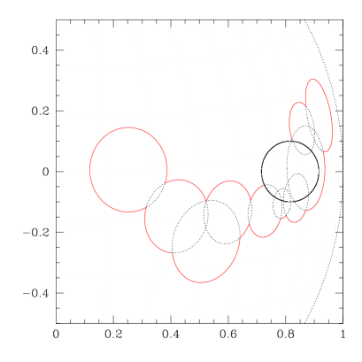
Figure 2: Left: the profile of a Jupiter planet overlapped to a complex spot region composed by ten spots. Black denotes integration on the planet border, red on the spots border. Dotted lines on the objects profiles denote invisible arcs, wherease those on the stellar surface denote stellar meridians and parallels. X and Y axis indicate the positions of the objects on the stellar surface normalized to the stellar radius. Right: the correspondent transit lightcurve during which the overlap of the planets with the spot region on the left side occurs, assuming an orbital period of 3 days for the planet and a rotation period of 9 days for the star.

5 Calculation of complex spot structures and occultations of spots by transiting bodies

It is now possible to provide the solution for the calculation of multiple spots overlap and occultations of spots by transiting bodies. For the latter case we note that Pál (2012) already provided the integrals to calculate the flux intercepted by a transiting body with the Kelvin-Stokes theorem. Given that in this work we provided the integrals for the case of spots with the same approach, it is sufficient to join the two results to obtain the general solution.

For convenience we will adopt here the same naming convention of Pál (2012) with only a slight useful modification. The projected shape of a spherical transiting body on the plane of the sky is a circle, while that one of a spot is an ellipse as it is possible to see for example from our definitions of $x$ and $y$. The interception of a circle with an ellipse yields in general a quartic equation which can be solved for each couple of objects with classic methods to find the roots (see below). The interception points define a set of arcs which are characterized with the notation $k:C\{k^{\prime},l\}$ where the number k indicates the circle or ellipse to which this l-th arc belongs and $C\{k^{\prime},l\}$ is a list of circles or ellipses that contain this arc. To identify if the arc is an arc of ellipse or circle we introduce here the modification that the indexes $k$, $k^{\prime}$ can be either negative or positive. All the arcs that define the boundary of integration $\partial S$ are those that are either corresponding to the stellar boundary (which we denote with the index 1), and are therefore of the form 1:$\{\}$ or those that are contained only in it (k:$\{1\}$). In the case in which we impose that the spots have a different contrast ratio $f$ to the stellar surface than the planets, (which are considered totally dark) we need to multiply the integrals on the spots arcs by the factor $f$ and we need also to consider in the integration the arcs of the planets contained inside the spots (see e.g. Fig.2) integrating on these arcs two times: the first on the same sense of the other planetary arcs that are not occulting the spots (to close the surface of the planet), and the second in the opposite sense (to close the surface of the spot region) multiplying this second integral by the factor $f$. Keeping this in mind if we consider like in Pál (2012) a set of arcs $a$ satisfying the above conditions which union is the boundary of integration $a\subset\partial S$ we can express the total integral in a compact form as

$$I=\sum_{a\in\partial S}(I(\phi_{a}^{2})-I(\phi_{a}^{1})),$$ (28)

where $\phi_{a}^{1}$ and $\phi_{a}^{2}$ are the extreme of integration along the generic arc a, as defined by the intersection points, and $I(\phi_{a}^{2})$, $I(\phi_{a}^{1})$ are the values of the appropriate integrals at these extreme points. If the arc a is denoted by a negative index k we will adopt our set of integrals reported in Eq. 26,27,28 (or Eq. 8,12,15). If the index k is positive or is the stellar boudary we will adopt the respective integrals calculated by Pál (2012).

To determine the values of $\phi_{a}^{1}$, $\phi_{a}^{2}$ located on an arc of a spot we proceed as follows. Considering a cartesian coordinate system $XYZ$ where the $X$ axis is now oriented toward the North and the $Y$ axis toward the East and the $Z$ axis is always along the line of sight, the coordinates of the center of a spot on the surface of the star will be given by a longitude angle $\beta_{0}$ measured from the $X$ axis toward the positive $Y$ axis, and by a co-latitude angle $\overline{\psi}$ measured from the sub-stellar point toward the plane of the sky. If $X_{p}$, $Y_{p}$, $Z_{p}$ denote the cartesian coordinates of the interception point in this system, the coordintes $x_{p}$, $y_{p}$, $z_{p}$ in the reference system of the spot shown in Fig. 1 are obtained inverting Eq.25, and by means of these coordinates it is easy to obtain the correspondent value of $\overline{\alpha}$ using the definitions in Section 2.

In such a way we can step from one arc to the other along the whole boundary to obtain the solution.

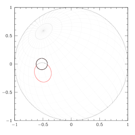
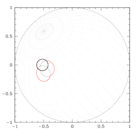
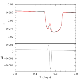
Figure 3: On the left side is visible a planet (in black) transiting in front of a single 10 degrees spot while on the middle panel transiting in front of a spot region composed by two 8 degrees spots offering to the observer the same projected area of the single spot. The rightmost panel shows the two resulting lightcurves (top) where the single spot model is denoted by the black line and the two spot model by the red line and the bottom panel shows the difference of the two lightcurves.

6 Examples

In Fig.3, we present one application where we first consider the overlap of a single spot, with angular dimension equal to 10 degrees and contrast ratio equal to 0.5 with a planet which radius is equal to 0.1 stellar radii. We additionally considered a stellar inclination angle of 50 degrees to the line of sight and a position angle (with respect to the y+ axis clockwise) of 320 degrees. The planet has an orbital period of 3 days transiting perfectly along the x-axis in the same sense of stellar rotation (P=30 days). This configuration produces the transit denoted by the black line in Fig.3 (rightmost panel). Alternatively we replace in Fig.3 (middle panel) the single spot with a double spot model composed by two spots each of 8 degrees angular dimension and contrast ratio equal to 0.5, creating overall an homogeneous spot region. The disposition of the two spots relative to each other is selected in such a way that the projected area they offer at the time of the transit is identical to that one of the single larger spot previously considered. The resulting transit is indicated by the red line in Fig.3 (rightmost panel), where in the bottom panel we present the difference between the two lightcurves. The result indicates that spot structure may appreciably affect the exact shape of the observed photometric signal, since variation of a few millimagnitudes with respect to the single spot model can be expected. A time resolution of around 1 min would be sufficient to resolve these structures. Depending on the extension of these regions spot crossing events may last also for a significant fraction of the transit event. Sub-millimag photometric precisions can be acheved today both from space and from the gound over these timescale. Studying accurately these events we can produce a tomographic analysis of the stellar surface.

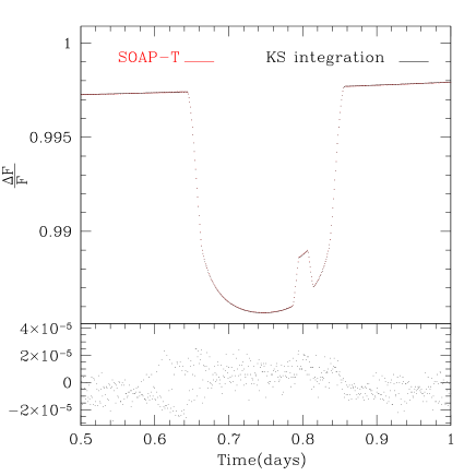
Figure 4: Top: A comparison between $KS$ integration (Kelvin-Stokes integration) and SOAP-T (Oshagh et al. 2013) for the case of a single circular spot crossed by a transiting planet. Bottom: the difference between the SOAP-T and the $KS$ lightcurve.

As another example, we compare in Fig.4 the output of $KS$ integration (Kelvin-Stokes integration, black points) with the SOAP-T numeric integrator result (Oshagh et al. 2013), considering the case of a single circular spot and a planet crossing in front of it. The average difference over the considered transit window is 8$\times\rm\,10^{-7}$ with a scatter equal to $10^{-5}$ denoting a good agreement between the two approaches.

7 Naked-eye spots

In Fig.5 we present an image of a spot region obtained by the Sacramento Peak Observatory of the National Solar Observatory in New Mexico. On top of the image we present a possible reconstruction of this region by means of the method presented in this work. Here the inner umbra region is modelled with two overlapping spots of equal contrast ratio, while the outer penumbra region is model by other two (lower constrast ratio) overlapping spots. To achieve the result in this case is sufficient to define some slightly different summation rules for the spots than considered before. For example spots of equal contrast ratio can be summed up homogeneously (thereby creating a larger spot region with the same contrast ratio of the components) whereas for spots with different contrast ratios we sum up algebrically the contrast ratio. In this way it is technically possible to create also very complex regions with sofisticated inner-side umbrae and outer side penumbrae.

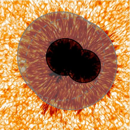
Figure 5: In the background is visible an image of a spot region composed by an inner umbra and a surrounding penumbra (image credit: Sacramento Peak Observatory of the National Solar Observatory in New Mexico). On top of the image a tentative reconstruction of the region using the method presented in this work.

8 The quartic

As explained above the interception between spot and planet profiles leads to a quartic equation for the roots. Here we report the explicit expression for the quartic coefficients as a function of the cosine of the angle $\psi$ between an interception point on the stellar surface and the line of sight. Defining $\overline{\psi}$ ($\overline{\psi_{p}}$) as the angle between the center of the spot (planet) and the line of sight, and $\Delta\phi$ as the angle between the spot and the planet centers (as seen from the center of the star on the plane of the sky), and introducing

$$p=\frac{\sin\overline{\psi}}{\sin\overline{\psi_{p}}}\sin\Delta\phi$$ (29)

$$q=\frac{\sin\overline{\psi}}{\sin\overline{\psi_{p}}}\cos\Delta\phi$$ (30)

$$\Delta\,r^{2}=\sin^{2}\overline{\psi_{p}}-r^{2}_{p}$$ (31)

where $r_{p}$ is the planet radius we have that the coefficients of the quartic are defined as

$$A\cos^{4}\psi+B\cos^{3}\psi+C\cos^{2}\psi+D\cos\psi+E=0,$$ (32)

$$A= -\frac{1}{4}(p^{2}+q^{2})$$ (33)

$$B= q\,\cos(\overline{\psi})$$ (34)

$$C= \frac{\Delta\,r^{2}+1}{2}(p^{2}+q^{2})-(\cos^{2}\overline{\psi}+q\,\cos\overline{\theta})$$ (35)

$$D= 2\cos\overline{\psi}\,\cos\overline{\theta}-q\cos\overline{\psi}(\Delta\,r^{2}+1)$$ (36)

$$E= -\frac{p^{2}\Delta\,r^{2}}{4}(\Delta\,r^{2}+2)-\frac{q^{2}}{4}(\Delta\,r^{2}+1)^{2}-$$

$$-\cos^{2}\overline{\theta}+q\,\cos\overline{\theta}(\Delta\,r^{2}+1)-\frac{p^{2}}{4},$$ (37)

We recall that four is the highest degree of a polynomial for which an algebric solution for the roots can be found. The solution was first provided by Lodovico Ferrari (1540).

9 Conclusions

In this work we presented the solution of the stellar spot problem obtained applying the Kelvin-Stokes theorem. The solution has been expressed in a closed form up to the second degree of the limb-darkening law and recursive expressions are provided for any polynomial expansion of the stellar intensity. We expressed the results both in the reference system of the spot and in a generic reference system arbitrarily oriented around the line of sight of the observer. Coupled with previous results on planets presented in Pál (2012) we have now a powerful technique to incorporate the effects of stellar activity into light-curve modelling including mutual photometric effects produced by planets with planets or planets with spots and allowing for the creation of complex and more realistic spot regions, and independent on the number, positions and dimensions of these objects.

The software implementation of the method described in this paper is made publically available directly at the following address http://eduscisoft.com/KSINT/ or through the link http://www.astro.up.pt/exoearths/tools.html. It is written in Fortran 95 and it has been tested on a Linux machine using a gfortran compiler. The program is called KSint ad can generate the lightcurve produced by an arbitrary combination of spots and planets.

Bibliography

Auvergne, M., Bodin, P., Boisnard, L., et al. 2009, A&A, 506, 411
Boisse, I., Bonfils, X., Santos, N. C., A&A, 545, 109
Budding 1977, Ap&SS, 48, 207
Collier Cameron 1997, MNRAS, 287, 556
Donati, J. F. & Brown, S. F. 1997, A&A, 326, 1135
Eker, Z. 1994, ApJ, 420, 373
Kipping, D. M., 2012, MNRAS, 427, 2487
Koch, D. G., Borucki, W. J., Basri, G., Batalha, N. M., Brown, T. M., Caldwell, D., Christensen-Dalsgaard, J., Cochran, W. D. et al. 2010, ApJL, 713, L79
Lanza, A. F., Bonomo, A. S., and Rodonó, M 2007, A&A, 464, 741
Oshagh, M., Boué G., Figueira, P., Santos, N. C., Haghighipour, N. 2013, A&A, 558, 65
Pál 2012, MNRAS, 421, 1825
Russell H. N. 1906, ApJ, 24, 1
Vogt, S. S. & Penrod, G. D. 1983, PASP, 95, 565
Walker, G., Matthews, J., Kuschnig, R., Johnson, R., Rucinski, S., Pazder, J., Burley, G., Walker, A. et al. 2003, PASP, 115, 1023