Carbon and Oxygen abundances across the Hertzsprung gap

Abstract

We derived atmospheric parameters and spectroscopic abundances for C and O for a large sample of stars located in the Hertzsprung gap in the Hertzsprung-Russell Diagram in order to detect chemical peculiarities and get a comprehensive overview of the population of stars in this evolutionary state. We have observed and analyzed high resolution spectra (R = 60 000) of 188 stars in the mass range 2 – 5 $M_{\odot}$ with the 2.7 m Harlan J. Smith Telescope at the McDonald Observatory including 28 stars previously identified as Am/Ap stars. We find that the C and O abundances of the majority of stars in the Hertzsprung gap are in accordance with abundances derived for local lower mass dwarfs but detect expected peculiarities for the Am/Ap stars. The C and O abundances of stars with ${T_{\text{eff}}}<6500\,$K are slightly lower than for the hotter objects but the C/O ratio is constant in the analyzed temperature domain. No indication of an alteration of the C and O abundances of the stars by mixing during the evolution across the Hertzsprung gap could be found before the homogenization of their atmospheres by the first dredge-up.

I. Introduction

The chemical evolution of normal mass stars from the main sequence (MS) to the ascent of the red giant branch (RGB) in the Hertzsprung-Russell Diagram (HRD) is complex and involves a sequence of processes that alter the composition and structure of their atmospheres. A key facet is the development of an expanding convective envelope that connects the outer layers of the atmosphere with deeper regions of nuclear burning. In the process the atmospheric abundances of several elements are altered and result in the abundance patterns typical for giant stars, i.e. a slight C deficiency that is accompanied by a N overabundance and a strong depletion of Li. Observational investigations consistently confirm these abundance patterns and the altered abundances of giants after the first dredge-up can be qualitatively predicted from the abundances of the corresponding normal mass dwarf progenitors.

Main sequence stars in the mass range 2 – 5 $M_{\odot}$ carry characteristics not exhibited by stars of about 1 $M_{\odot}$ which provide the majority of G and K giants. The higher mass stars have a larger range in rotational velocities whereas solar mass main sequence stars are all slow rotators; a sharp break in projected rotational velocity occurs at about 1.3 $M_{\odot}$ (Kraft 1967). In addition, the main sequence domain of the higher mass stars is populated with a variety of chemically-peculiar stars of spectral types Ap and Am for which diffusion of elements is considered to have distorted the composition of their atmospheres. A different group of chemically-peculiar stars can be found on the other side of the Hertzsprung gap in the form of weak G band stars (wk Gb stars), a rare group of early G and K giants of slightly sub-solar metallicity that show unusually large underabundances of C. While the origin of the chemical peculiarities of the Am/Ap stars can be explained reasonably well by theoretical models, the exact cause for the wk Gb abundance anomalies is still subject to speculation.

For these stars in the higher mass range, the crossing of the Hertzsprung gap marks an essential period in their evolution and the mechanisms that affect the distribution of elements in their atmospheres, culminating in the first dredge-up, effectively determine the abundance patterns of their descendants on the giant branch. However, apart from determinations of abundances for Li and selected elements (Wallerstein et al. 1994; Hiltgen 1996; de Laverny et al. 2003), to our knowledge, no extensive abundance analysis of a larger number of stars in this evolutionary stage has been performed yet. Especially the abundances of the basic elements C, N, and O are of interest, since these elements are altered by the nuclear processes involved in the energy production via the CNO-cycle and are different for dwarf and giant stars. These elements are therefore the key indicators to analyse abundance patterns, identify and investigate chemical peculiarities, and get a comprehensive picture of the characteristics of stars in the Hertzsprung gap. The determination of abundances of these and other elements necessarily faces the difficulty that spectra of many stars will be greatly rotationally broadened thus complicating, even thwarting, an abundance analysis. Nonetheless, in this paper, we aim to provide a detailed analysis of C and O abundances of a large sample of stars in the mass range 2 – 5 $M_{\odot}$ that are located in the Hertzsprung gap in the HRD.

II. Observations and target selection

We compiled a sample of target stars from the Hipparcos catalog (van Leeuwen 2007). The primary selection criterion was their position in the Hertzsprung-Russell Diagram (HRD). Effective temperatures were calculated from B-V colors with the calibrations from Alonso, Arribas, & Martínez-Roger (1999) and luminosities were determined with the Hipparcos parallaxes and V magnitudes. We selected stars with masses between 2 and 5 $M_{\odot}$ by comparison with evolutionary tracks from Bertelli et al. (2008, 2009) and a lower temperature limit of $\log({T_{\text{eff}}})>\log(3.72)$. The sample was furthermore restricted to stars with small errors in their parallaxes and declinations $>-20^{\circ}$. For a first set of observations, stars with an error in their parallaxes of less or equal than 20% of the actual parallax and a right ascension (RA) in the range of 4 – 20 h were observed. This sample was complemented with additional observations of objects with a parallax error of less or equal than 50% of the parallax in order to better cover the less populated area of higher masses (see Section III.6). For the second sample, stars with a right ascension between 20 – 11 h were accessible. It should be noted that with this target selection it is impossible to detect the direction of the transition of a star through the Hertzsprung gap and to distinguish, e.g. a main sequence star on its way to the giant branch from a pulsating horizontal branch star or a post-AGB star.

We observed 188 stars with the 2.7 m Harlan J. Smith Telescope at the McDonald Observatory. The telescope was equipped with the Robert G. Tull Cross-Dispersed Echelle Spectrograph (Tull et al. 1995) and a Tektronix 2048 x 2048 pixel CCD detector. The stars were observed in what we deem the standard (std) setup centered on 5060 Å in order 69. This setup up was chosen in order to cover as many of the interesting spectral lines as possible. The observations covered a wavelength range of 3 900 – 10 000 Å with a resolving power of $\text{R}\equiv\lambda/\Delta\lambda=60\,000$. The observations are listed in Table 1. Unless noted otherwise the spectra were reduced in a multiple step procedure. First flat field and bias corrections were applied. Then the echelle spectra were extracted and wavelength calibrated using ThAr-lamp comparison exposures taken before or after the observations. The different spectral orders were combined and continuum normalized. All tasks were performed using the IRAF package .

Table 1Observation log of analyzed spectra .

HIP	HD	V [mag]	Obs. date	$t_{exp}$ [s]	SNR
HIP 8066	HD 10497	6.9	2013 Nov 30	840	252
HIP 11115	HD 14542	7.1	2013 Nov 30	1020	232
HIP 13004	HD 17086	6.6	2013 Nov 30	660	190
HIP 13036	HD 17245	6.6	2013 Nov 30	720	284
HIP 16001	HD 21085	7.2	2013 Nov 30	1140	250
HIP 16203	HD 21483	7.1	2013 Nov 30	1080	175

Note. — Table 1 is published in its entirety in the electronic edition of The Astrophysical Journal. A portion is shown here for guidance regarding its form and content.

III. Parameter determination

In order to determine reliable effective temperatures and atmospheric parameters we utilized a variety of different techniques that are described in the following.

III.1. Fe line equivalent widths

Atmospheric parameters were derived from Fe line equivalent widths (EWs). We will refer to these parameters as spectroscopic keeping in mind that some of the other methods also rely on the observed spectra. The equivalent widths of 37 Fe i and 9 Fe ii lines were measured with the IRAF routine splot whenever possible. Many of the stars are fast rotators. In some cases a de-blending of the lines was necessary, in other cases no determination of equivalent widths was possible at all. The ${\log gf}$ values and excitation potentials were taken from Ramírez & Allende Prieto (2011). The line list and measured equivalent widths were taken as an input for the spectral synthesis code MOOG (Sneden 1973). One-dimensional (1D), plane-parallel input model atmospheres in local thermodynamic equilibrium (LTE) were interpolated from a grid of models from Castelli & Kurucz (2004). The abundances of the computed Fe lines for a given set of parameters were force-fitted to match the measured EWs. NLTE effects that could alter the determination of Fe abundances and thus affect the stellar parameters are negligible for stars in our temperature and metallicity range (Lind, Bergemann, & Asplund 2012). For the right set of parameters three conditions are fulfilled: The determined Fe abundance or metallicity is independent of the excitation potential (excitation equilibrium), there is no trend between Fe abundance and reduced EWs (EW/$\lambda$), and the abundances determined from Fe i and Fe ii lines are equal (ionization equilibrium). The parameters are found by minimizing a $\chi^{2}$ function that is a quadratic form constructed from the conditions mentioned above. We use the Nelder-Mead or Downhill Simplex algorithm to perform the minimization procedure. Our implementation follows closely the method described in Saffe (2011). The error for ${T_{\text{eff}}}$ was estimated to be the temperature difference that would produce a difference in Fe abundances of low and high excitation potential lines that is larger than the standard deviation ($\sigma$) of the determined Fe abundance. In a similar way, the uncertainty for the microturbulence ${v_{t}}$ can be derived as the difference in ${v_{t}}$ that produces Fe abundance differences for different reduced equivalent widths that are larger than $1\sigma$ of the Fe abundance. The error for the surface gravities is assumed to be the difference in logg that produces a difference in the Fe abundances derived from Fe i and Fe ii lines that is larger than the standard deviation of the Fe abundance. The error of the metallicity is calculated from the difference in the Fe i and Fe ii abundances combined with the standard deviations for the Fe abundance determinations for Fe i and ii lines added in quadrature. The procedure was tested for Fe line EWs measured in a solar spectrum observed with the same setup as the program stars. We obtain ${T_{\text{eff}}}=5756\pm 86\,\text{K}$, ${\log g}=4.41\pm 0.11$, $[\text{Fe/H}]=-0.01\pm 0.07$, and ${v_{t}}=0.76\pm 0.97\,\text{km s${}^{-1}$}$. Since the effective temperature is the most important parameter the determined spectroscopic temperatures were adjusted by adding the difference of 21 K compared to the expected solar temperature of 5777 K. The spectroscopic parameters are summarized in Table 2.

Table 2Spectroscopic parameters for the program stars.

object	${T_{\text{eff}}}$ [K]	$\sigma$	${\log g}$ [cm s-2]	$\sigma$	[Fe/H]	$\sigma$	${v_{t}}$ [km s-1]	$\sigma$
HIP 13036	4690	156	1.96	0.28	-0.35	0.37	1.38	0.27
HIP 27380	5963	69	0.68	0.20	-0.24	0.44	2.70	1.30
HIP 30735	7269	244	2.31	0.32	-0.08	0.28	3.13	1.56
HIP 31164	5471	171	3.94	0.23	-0.25	0.20	1.68	0.37
HIP 32063	5101	83	3.30	0.21	-0.19	0.16	0.87	0.16
HIP 32404	8192	96	2.40	0.20	0.49	0.31	2.65	19.27

Note. — Table 2 is published in its entirety in the electronic edition of The Astrophysical Journal. A portion is shown here for guidance regarding its form and content.

III.2. Full spectrum fitting

We determined atmospheric parameters with the full-spectrum fitting University of Lyon Spectroscopic Analysis Software package ULySS (Koleva et al. 2009). The observed spectra were fitted against stellar spectra models based on the 3.2 version of the ELODIE library (Prugniel & Soubiran 2001) represented by an interpolator (Prugniel et al. 2011). The ELODIE library consists of echelle spectra in the wavelength range $3\,900-6\,800\,\AA\,$ with a spectral resolutions of $\text{R}=42\,000$, containing stars with spectral types from O to M. The interpolator represents a low resolution ($\text{R}=10\,000$) version of the library and consists of polynomial expansions of each wavelength element in powers of $\log({T_{\text{eff}}})$, ${\log g}$, [Fe/H], and $f(\sigma)$, where $f(\sigma)$ is a function of the rotational broadening parameterized by the standard deviation of a Gaussian. The fitting procedure performed by ULySS interpolates a spectrum, convolves it with a Gaussian and multiplies it with a polynomial to derive the best fit to the observation. The free parameters of the minimization procedure are the atmospheric parameters ${T_{\text{eff}}}$, ${\log g}$, and [Fe/H], as well as two parameters for the Gaussian, the systemic velocity $v_{sys}$ and the dispersion $\sigma$, and the coefficients of the polynomial. The systemic velocity corrects for uncertainties in the radial velocities of the stars, the dispersion includes both the instrumental broadening and the effect of rotation.

Before the actual fitting, the observed spectra were adapted to the resolution of the interpolated spectra. We have to ensure that the model has in fact a higher spectral resolution than the observation (Prugniel et al. 2011). This is necessary because it is convolved with a Gaussian representing a line-of-sight-velocity distribution (LOSVD) during the analysis, but not always guaranteed because the effective spectral resolution of the spectra is determined by the rotational broadening and the dispersion of the instrumental broadening. The observed spectra were therefore convolved with a Gaussian with a fwhm that is higher than necessary to match the low spectral resolution of the interpolated spectra. The physical broadening of the observed spectra due to their rotational velocities can in principle directly be determined from ULySS if a suitable line-spread function (LSF) is injected that takes into account the varying relative resolution between the observation and model with wavelength. However, using an exact LSF has only a negligible influence on the derived atmospheric parameters (Wu et al. 2011) and we derived rotational velocities for the program stars by comparing the measured dispersion velocities with a list of literature values of $v\sin i$ for our stars from different authors (Royer et al. 2002; Schröder, Reiners, & Schmitt 2009; Bernacca & Perinotto 1970; Abt & Morrell 1995; Massarotti et al. 2008). This calibration was restricted to stars with errors in the dispersion of less than 30% of the actual value. The result of the calibration can be seen in Figure 1. The solid line shows the fit of a weighted second order polynomial to the observations with the errors of the dispersion velocities taken as weights. The rotational velocities are then derived from the dispersion velocities X with the following correlation: $0.556-0.008\cdot\text{X}^{2}+2.386\cdot\text{X}$.

The normalized spectra of our program stars were fitted in the wavelength range covered by the ELODIE spectra. To avoid the introduction of fitting errors caused by the echelle gaps of our spectra we fitted the wavelength ranges of each order separately. The final temperature for a star was derived by calculating a sigma-clipped weighted average over the results obtained from all fitted orders, taking the $\chi^{2}$ values determined by ULySS as weights. The error for the temperature is taken as the sigma-clipped and weighted standard deviation. Analogously we derive values for ${\log g}$ and [Fe/H] and their errors.

Table 3Parameters for the program stars derived with ULySS.

object	${T_{\text{eff}}}$ [K]	$\sigma$	${\log g}$ [cm s-2]	$\sigma$	[Fe/H]	$\sigma$	disp. vel [km s-1]	$\sigma$
HIP 8066	7602	162	2.90	0.71	0.12	0.10	14.21	2.03
HIP 13004	8250	213	2.48	0.61	-0.03	0.09	14.97	2.61
HIP 13036	5002	47	2.30	0.14	-0.23	0.14	6.97	1.49
HIP 16001	8637	152	2.10	0.34	-0.10	0.08	3.37	3.37
HIP 20000	8693	442	1.85	0.67	-0.58	0.99	83.05	105.78
HIP 21446	7782	1559	3.06	1.70	-1.25	1.12	196.88	51.19

Note. — Table 3 is published in its entirety in the electronic edition of The Astrophysical Journal. A portion is shown here for guidance regarding its form and content.

Again, atmospheric parameters were derived with a solar spectrum. We obtained ${T_{\text{eff}}}=5743\pm 73\,\text{K}$, ${\log g}=4.32\pm 0.14$, and $[\text{Fe/H}]=-0.01\pm 0.04$. The difference of 34 K compared to the expected solar temperature was added to the derived ${T_{\text{eff}}}$ for our stars. The parameters derived with ULySS agree well with the spectroscopic ones. The mean difference in ${T_{\text{eff}}}$ is $\sim$20 K with a $\sigma$ of $\sim$90 K for stars for which both temperatures estimates were available. For ${\log g}$ and [Fe/H] the differences are equally small with $0.25\pm 0.28$ and $0.08\pm 0.14$. The atmospheric parameters derived with ULySS can be found in Table 3.

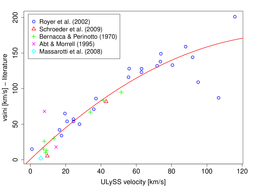
Figure 1.— Rotational velocities for some of our program stars taken from different literature sources plotted against the dispersion velocities derived with ULySS.

III.3. H-$\alpha$ line fitting

The H-$\alpha$ line was used to determine effective temperatures for the program stars by fitting theoretical synthetic spectra to the observations as described in Barklem et al. (2002). Problems can arise due to the strong wings of the line that can extend over a whole spectral order and make the exact determination of the continuum difficult. Therefore, a special normalization is necessary. The main idea of the procedure is to determine the continuum of neighboring orders that are not affected by the wings of the line and to interpolate the continuum for the order containing H-$\alpha$. The procedure is described in more detail in Barklem et al. (2002). A grid of Barklem’s H-$\alpha$ profiles with different temperatures was used and a reduced $\chi^{2}$ value that quantifies the difference between observation and synthetic spectrum was derived for each ${T_{\text{eff}}}$. The $\chi^{2}$ function was calculated as the sum of the squared differences between observed and calculated fluxes divided by the statistical error of the fluxes (1/SNR) for regions of the profile that are not affected by metal lines. $\chi^{2}$ values for temperatures in the grid and two different values for ${\log g}$ were determined. The temperature grid ranges from 4 400 to 7 500 K with values for ${\log g}$ of 3.4 and 3.0. The choice of ${\log g}$ is influenced by the previously determined spectroscopic value for ${\log g}$ but does not have any significant impact on the derived result for ${T_{\text{eff}}}$. The best-fit ${T_{\text{eff}}}$ is obtained by minimizing the set of $\chi^{2}$ values and fitting a parabola to the seven points closest to the minimum of the $\chi^{2}$ function. The error of the temperature determination is given as the error of the fit. The method was applied to a solar spectrum and the parameters for the normalization procedure were adjusted to get as close to the expected solar temperature as possible. The systematic error of our procedure was then estimated by determining the solar temperature with the FTS atlas (Kurucz et al. 1984) that was used by Barklem et al. (2002). For the atlas our method yields a slightly higher temperature of ${T_{\text{eff}}}=5799\pm 3\,\text{K}$ and the difference of 22 K to the expected solar ${T_{\text{eff}}}$ was subtracted from the H-$\alpha$ temperatures of the program stars.

Unfortunately, for our setup (see Section II) the H-$\alpha$ line is located at the edge of an order. Therefore, the blue wing of the line can not be used. Also, we restrict the fit to the upper part of the lines, since the cores are not formed in the photosphere and are therefore affected by NLTE effects. Due to these difficulties, H-$\alpha$ temperatures could only be determined for a limited number of stars. The derived temperatures, however, agree with the spectroscopic ones with a mean difference of $\sim$30 K but show a larger standard deviation of $\sim$200 K. The temperatures derived by the H-$\alpha$ line fitting are summarized in Table 4.

III.4. Photometric

Effective temperatures from photometric colors were derived using the calibration of Ramírez & Meléndez (2005). The intention was to use as many colors as possible but to consider only photometric data of high quality. The main source for photometric data used in the analysis was the General Catalogue of Photometric Data (GCPD; Mermilliod, Mermilliod, & Hauck 1997). It contains data for many different photometric systems including UBV, uvby, Vilnius, Geneva, and DDO. In addition ground-based V magnitudes included in the Hipparcos-Tycho catalog (ESA 1997) and infrared colors from the Two Micron All Sky Survey (2MASS), if the observations were not saturated, were used. Some of the program stars have companions that heavily influence specific photometric colors. In these cases the colors that were most affected were excluded from the temperature determination. Close binaries and stars with photometric data of insufficient quality were rejected. Overall, photometric temperatures could be derived for 142 stars. The average of all available temperatures was adopted as the photometric ${T_{\text{eff}}}$ and the standard deviation taken as its error. In cases where only one temperature could be derived, we assume an error of 100 K. For all stars the metallicity was assumed to be solar in the calculations.

The photometric temperatures are close to the spectroscopic temperatures with a mean difference of 90 K but show some scatter with a $\sigma$ of 220 K. The photometric temperatures are calculated with an estimated reddening (see Section III.6).

In addition to the temperatures, a photometric calibration was used to calculate ${\log g}$ values. We used the derived masses for our stars (see Section III.6), the V magnitudes, the adopted temperatures (see Section III.5), and the relation

$${\log g}=0.4(M_{\text{bol}}+M_{\text{bol}\,\odot})+{\log g}_{\odot}+4\log\left(\frac{{T_{\text{eff}}}}{{T_{\text{eff}\,\odot}}}\right)+\log\left(\frac{M}{M_{\odot}}\right),$$

where $M_{\text{bol}}=M_{\text{V}}+BC$. We take ${T_{\text{eff}\,\odot}}=5780\,\text{K}$, ${\log g}_{\odot}=4.44$, and $M_{\text{bol}\,\odot}=4.75\,\text{mag}$, as the solar parameters. The photometric ${\log g}$ agree with the spectroscopic ones, showing a mean difference of $0.30\pm 0.35$. Photometric temperatures and ${\log g}$ values are shown in Table 4.

Table 4H_α and photometric parameters for the program stars.

object	${T_{\text{eff}}}$ Hα [K]	$\sigma$	${T_{\text{eff}}}$ [K]	$\sigma$	${\log g}$ [cm s-2]	$\sigma$
HIP 8066			6997	89	2.79	0.32
HIP 13004			8221	100	2.74	0.35
HIP 19529			7570	201	3.10	0.26
HIP 19823			6111	206	2.39	0.15
HIP 21084			7619	100	3.09	0.36
HIP 21446			7532	547	3.00	0.20

Note. — Table 4 is published in its entirety in the electronic edition of The Astrophysical Journal. A portion is shown here for guidance regarding its form and content.

III.5. Adopted parameters

We adopted the mean of all available temperature determinations as the effective temperature for our program stars and take the standard deviation as the error. The number of available temperatures varies and mainly depends on the rotational broadening of the lines in the spectrum. In almost all cases, however, a photometric and ULySS temperature can be used. If only one temperature is available the error of the individual temperature determination was also taken as the uncertainty for the final adopted temperature. Note that the errors in the individual temperatures derived with the full spectrum fitting method (Section III.2) for stars that are fast rotators can be quite large. The agreement with the photometric temperatures for objects where at least two temperatures could be derived, however, justifies the use of the ULySS temperatures also in cases where it is the only temperature indicator available. Furthermore, we include the uncertainty in temperature in the error determination of the derived elemental abundances (see Section IV). For the surface gravities the mean and standard deviation of the values from the spectroscopic and ULySS determination was taken as the adopted value and its error, whenever possible. If only one of these ${\log g}$ could be determined again the error of this determination was taken as the adopted error. For stars with only photometric temperatures the photometric ${\log g}$ and the associated error was taken. Similarly, the mean of the metallicities derived from the spectroscopic and ULySS determination was taken as the adopted [Fe/H] and the standard deviation as its error. A solar metallicity was assumed for stars with only photometrically determined ${T_{\text{eff}}}$ and ${\log g}$. An exception was made for HIP 95497 (RR Lyr) for which we take a metallicity of -1.45 dex. This is the mean of the two metallicities from Kolenberg et al. (2010) and Takeda et al. (1999), see Section IV.3. The microturbulence and its error were taken from the spectroscopic determination. For stars with no derived microturbulence we assume ${v_{t}}=1.8\pm 0.35\,\text{km s}^{-1}$. Furthermore, the rotational velocities from our calibration described in section III.2 were adopted. All adopted atmospheric parameters can be found in Table 5 and histograms of the adopted values for ${T_{\text{eff}}}$, ${\log g}$, and [Fe/H] are shown in Figure 2.

Figure 2.— Histograms of the adopted parameters of our program stars.

Table 5Adopted atmospheric parameters for the program stars. The fourth column shows the number of different temperature indicators that were used in the determination of ${T_{\text{eff}}}$.

object	${T_{\text{eff}}}$ [K]	$\sigma$	n	${\log g}$ [cm s-2]	$\sigma$	[Fe/H]	$\sigma$	${v_{t}}$ [km s-1]	$\sigma$	$v_{\sin i}$ [km s-1]	$\sigma$
HIP 8066	7300	428	2	2.90	0.71	0.12	0.10	1.80	0.35	32.84	2.03
HIP 13004	8236	21	2	2.48	0.61	-0.03	0.09	1.80	0.35	34.47	2.61
HIP 13036	4846	221	2	2.13	0.24	-0.29	0.08	1.38	0.27	16.80	1.49
HIP 16001	8637	152	1	2.10	0.34	-0.10	0.08	1.80	0.35	8.51	3.37
HIP 19529	7570	201	1	3.10	0.26	0.00	0.25	1.80	0.35	89.72	109.68
HIP 19823	6111	206	1	2.38	0.15	0.00	0.25	1.80	0.35	10.69	6.35

Note. — Table 5 is published in its entirety in the electronic edition of The Astrophysical Journal. A portion is shown here for guidance regarding its form and content.

The first panel clearly shows the separation of the sample into two groups with temperatures below and above $\sim 6500\,\text{K}$. This separation illustrates the limited number of stars than can be found in the center of the Hertzsprung gap.

III.6. Reddening, Mass, and Luminosity

The reddening of our stars was estimated according to the procedure described in Luck & Heiter (2007). First, the reddening of the stars was calculated with the EXTINCT code from Hakkila et al. (1997), using the position of the objects and the distances calculated from the parallaxes of the new reduction of the Hipparcos catalog (van Leeuwen 2007). Then, the reddening for the reddening-free Local Bubble, i.e. all reddening calculated for a distance of 75 pc, was subtracted.

Luminosities for the program stars were calculated with the Hipparcos parallaxes and the GCPD visual magnitudes and their errors, whenever possible. For stars with no GCPD V magnitudes, Hipparcos magnitudes and their errors were used. We take the adopted temperatures and applied a bolometric correction according to Alonso et al. (1999). With the luminosities and adopted temperatures, the program stars can be placed in the HRD. This is shown in Figure 3.

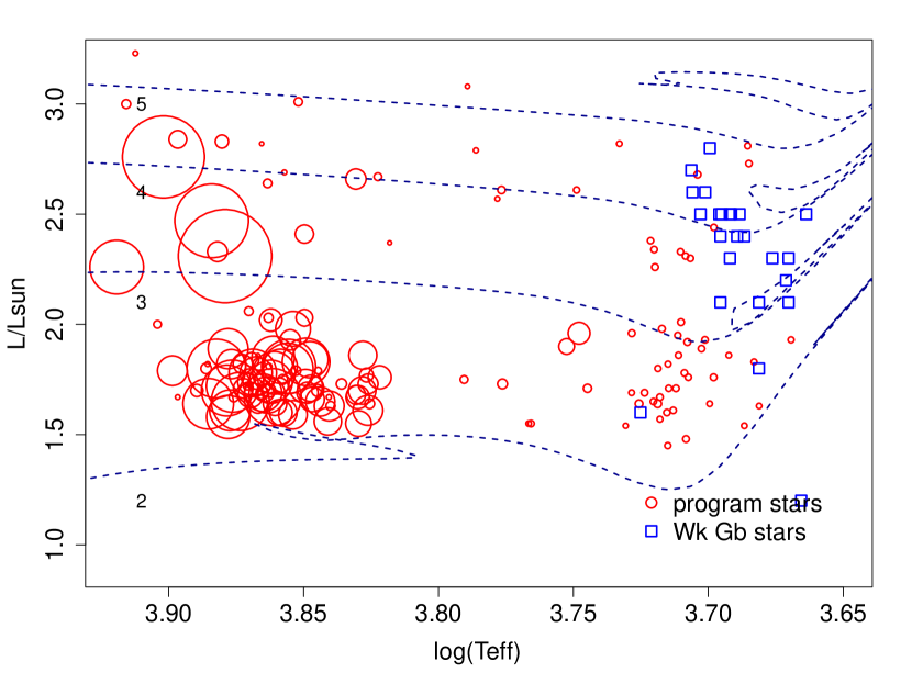
Figure 3.— Program stars in the HRD. The circle size correlates with the rotational velocities of the objects. Evolutionary tracks, labeled with the respective stellar mass in $M_{\odot}$, were calculated by Bertelli et al. (2008, 2009) for a solar composition ($\text{Z}_{\odot}=0.017$, $\text{Y}_{\odot}=0.260$).

The masses of the stars were determined by interpolating between the evolutionary tracks from Bertelli et al. (2008, 2009). We rely on the evolutionary tracks for a solar composition ($\text{Z}_{\odot}=0.017$, $\text{Y}_{\odot}=0.260$). Changing the metallicity does not significantly affect the masses of our objects. The masses of the program stars are almost exclusively in the range $2-5\,M_{\odot}$ with a mean mass of $2.51\pm 0.76\,M_{\odot}$. To check the influence of the chosen evolutionary tracks, masses were also derived from evolutionary tracks from Demarque et al. (2004). These masses were higher by $0.31\pm 0.21\,M_{\odot}$. The lower number of objects above $3\,M_{\odot}$ in our sample is due to the constraints from the target selection and the generally low population of stars in this area of the HRD in the Hipparcos catalog. The results for the mass and luminosity determination are summarized in Table 6.

Table 6Masses, distances, and luminosities of the program stars.

object	plx [mas]	$\sigma$	d [pc]	$\sigma$	$\log$ L	$\sigma$	M [$M_{\odot}$ ]	$\sigma$
HIP 8066	1.97	0.66	508	170	2.64	0.29	3.61	0.68
HIP 13004	1.48	0.58	676	265	3.00	0.34	4.44	1.00
HIP 13036	2.16	0.56	463	120	2.81	0.23	4.58	0.68
HIP 16001	1.33	0.52	752	294	2.85	0.34	4.01	0.88
HIP 19529	2.62	0.71	382	103	2.31	0.24	2.91	0.43
HIP 19823	2.33	0.33	429	61	2.79	0.12	4.10	0.32

Note. — Table 6 is published in its entirety in the electronic edition of The Astrophysical Journal. A portion is shown here for guidance regarding its form and content.

IV. Abundances

The abundance analysis focuses on the elements that are key constituents of the CNO-cycle and are altered in giant stars after the first dredge-up: C and O. The focus on these elements is also founded on the number of spectral lines that are accessible for the two elements. Unfortunately, the determination of a N abundance is prevented by the lack of usable N lines in our spectra. For the abundance analysis described below the EWs of suitable lines were measured with the IRAF routine splot. The lines were de-blended when necessary and corrected for the influence of other elements. The abundances were then determined with MOOG using a model atmosphere with the adopted parameters as input. In addition to the program stars the EWs of lines in a solar spectrum observed with the same setup were measured and a solar abundance for each line was derived. The solar abundances were used to determine relative abundances for our elements of interest.

IV.1. Carbon

We use three C i lines at 5052, 5380, and 6587 Å  as the main indicators for the C abundance. The 5052 Å  line is close to an Fe i and a Cr i line and has to be carefully de-blended. The signal to noise ratio of our spectra is sufficiently high but difficulties are caused by the high rotational velocities in some stars. The line at 6587 Å  is very weak but can nevertheless be used to derive abundances for a large fraction of our objects. For all three lines the excitation potentials and ${\log gf}$ values as published in Asplund et al. (2005) were taken. With the observed solar spectrum and solar parameters of ${T_{\text{eff}\,\odot}}=5780\,\text{K}$, ${\log g}_{\odot}=4.44$, the C abundances of 8.39 , 8.41, and 8.32 for the lines at 5052, 5380, and 6587 Å  were derived.

We use the C i line at 8335 Å  as an additional abundance indicator. However, since this line can be severely blended with a telluric component it could not be used for the majority of our objects. In two cases, for HIP 81933 and HIP 82093, the 8335 Å  line is the only indicator for the C abundance. For this line a solar abundance of 8.29 was obtained. Again, the excitation potential and ${\log gf}$ value from Asplund et al. (2005) were used.

The C i triplet at 9078, 9088, and 9094 Å  is present in our spectra but strongly blended by telluric lines that make it impossible to derive accurate abundances from them. The C i line at 9111 Å  is strong enough in our spectra. However, the line is close to a Fe i line and in many cases blended. Furthermore, it suffers from severe NLTE effects (Przybilla, Butler, & Kudritzki 2001) and was therefore not used for an abundance determination. The atomic data for the lines used for the C abundance determination are presented in Table 8.

The C abundance is derived as the mean from the abundances of the individual lines and is shown in Table 7. The error is given as the standard deviation. In cases where only the abundance of one line was available this error is assumed to be 0.1 dex. Overall, C abundances for 66 stars could be derived with the described method. The other stars in the sample show strongly broadened lines that prevent the measurement of individual EWs. We estimated the effect of a change in temperature on the C abundances. Changing ${T_{\text{eff}}}$ by 100 K leads to a change in the C abundance of less than 0.1 dex. Using the derived uncertainties for the adopted temperatures an additional temperature dependent error was calculated for the C abundance of each star and included in the determination of the error of [C/H]. Luck & Heiter (2006, Figure 3) showed that the C abundances from our three C i lines gave very similar results for stars with ${T_{\text{eff}}}\geq 5250\,$K but at lower temperatures the 5380 Å  line gave higher abundances presumably due to an unknown blend and the 5052 Å  line gave lower abundances due to interference from the wing of a Fe i line. Few of our stars (Figure 2) have temperatures cooler than 5250 K and there are no significant differences in the abundances derived from the 5380 and 5052 Å  line in these cases. For the cool stars, the primary C abundance indicator chosen by Luck & Heiter was a C₂ Swan band feature at 5135 Å. This feature is present in our coolest stars but disappears for hotter temperatures.

We used the stars with C abundances derived from the individual lines to infer C abundances for the rest of the stars in our sample that exhibit high velocity broadening. For this purpose the strength of the CH G band was measured for each star by integrating the flux over the wavelength range $4290-4320\,\AA$. Then, a weighted multivariate linear model was calculated that sets the C abundance in relation to the measured strength of the G band and the atmospheric parameters ${T_{\text{eff}}}$, ${\log g}$, and [Fe/H], taking the previously determined errors in the C abundances as weights. The model was trained with the sample of stars for which both C abundances from the individual lines and the strength of the CH G band could be determined. The Am/Ap stars (see Section IV.4) in the sample were excluded in the calculation of the model. The mean residual of the resulting model is $-0.01\pm 0.31$ dex. The model was used to predict the C abundances for the stars with high rotational velocities. Finally, a metallicity dependent correction was added to adjust the trend with [Fe/H] and account for the fact that many of the high rotators have high metallicities that extend beyond the range of the training set. The strength of the G band depends on ${T_{\text{eff}}}$ and gets weaker for increasing temperatures. Due to the high rotation in the hottest stars in our sample it is impossible to visually detect if the absorption in that region is due to CH or other metal lines. A comparison with synthetic spectra calculated with varying C abundances in our parameters range, however, suggests that the contribution of CH gets negligible for stars hotter than 7500 K and we restrict our G band abundance determination to temperatures cooler than that. The error for the abundances derived in this way is estimated to be 0.32 dex and consists of the standard deviation of the residuals and the mean error of the C abundances from the training set added in quadrature. The C abundances derived in this way are also shown in Table 7. For the C abundances derived from the individual lines [C/H] is the mean of the abundances relative to the solar abundances of each line. For the C abundances determined with the G band [C/H] is the calibrated C abundance relative to the mean solar C abundance (8.35).

Table 7C abundances for the program stars. The last column indicates the method used for the abundance determination (l = lines, G = CH G band model). See text for details.

object	C	$\sigma$	[C/H]	$\sigma$	method
HIP 8066	8.26	0.32	-0.09	0.53	G
HIP 13036	7.82	0.39	-0.58	0.43	l
HIP 16001	8.75	0.03	0.37	0.15	l
HIP 19823	7.84	0.13	-0.54	0.27	l
HIP 27380	7.70	0.09	-0.67	0.19	l
HIP 27747	8.11	0.32	-0.24	0.43	G

Note. — Table 7 is published in its entirety in the electronic edition of The Astrophysical Journal. A portion is shown here for guidance regarding its form and content.

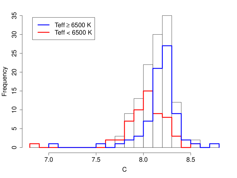
Figure 4.— C abundances for our program stars.

In Figure 4 a histogram of the C abundances derived with both methods is shown. Stars with temperatures below 6500 K show in general smaller C abundances than the group of stars with higher temperatures.

In Figure 5 the C abundances are compared to data for nearby dwarfs of spectral types F-K from Luck & Heiter (2006), covering a ${T_{\text{eff}}}$ range from $4100-7141\,\text{K}$. Luck & Heiter derived their abundances by synthesizing the C i 5380 and 6578 Å  lines and a feature of the C₂ Swan system at 5135 Å.

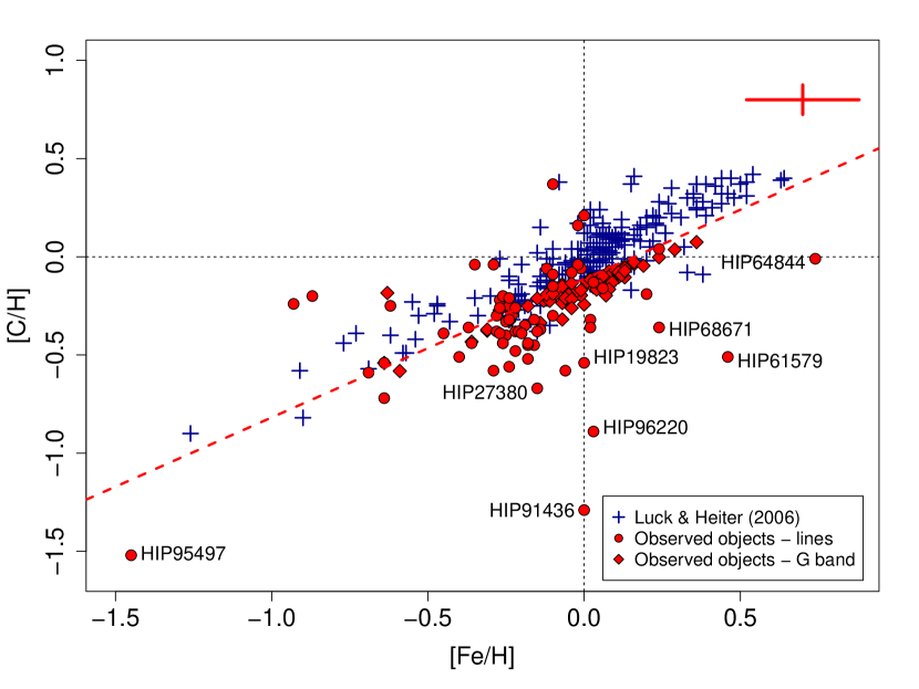
Figure 5.— Carbon abundance relative to solar for our program stars. The cross indicates the typical error of the abundances derived with the individual lines. The dashed line is a linear fit to the stars from Luck & Heiter (2006) shifted by an offset of -0.1 dex in [C/H], see text for details.

The offset of our [C/H] – [Fe/H] trend from that defined by Luck & Heiter’s F-K dwarfs arises presumably from systematic differences in the [C/H] and/or the [Fe/H] abundances: a difference of -0.1 dex in [C/H] (see Figure 5) is shown to reconcile the two trends but a similar adjustment to [Fe/H] achieves a comparable reconciliation. Unfortunately, the two samples do not have stars in common so that direct determinations of the systematic differences are not possible. Differences at the level of 0.1 dex seem inevitable when analyses of different samples are undertaken by different groups: different lines with different $gf$-values and different families of model atmospheres, different basic defining parameters are some of the key factors.

Luck & Heiter compare their [Fe/H] measurements with results from eight different analyses by other authors and find mean differences from -0.01 to +0.07 dex in considering large numbers of common stars. For [C/H], they find a mean difference of -0.07 dex from 62 stars in common with Ecuvillon et al. (2004) where the difference is +0.1 dex with our sample. Our sample is systematically warmer than Luck & Heiter’s and, thus, non-LTE effects may introduce an offset between the C and/or the Fe abundances. The lines used in our analysis are generally not known to be severely affected by non-LTE effects but small corrections in the order of $\approx 0.04$ dex were found by Asplund et al. (2005) for 3 of the lines considered here. In light of the fact that only large [C/H] differences would be an indicator for a possible connection between the sample stars and peculiar stars on the giant branch like the wk Gb stars, the offset of 0.1 dex is irritating but not fatal. We therefore refrained from performing a detailed analysis of possible non-LTE effects. Moreover, the comparable comparison for [O/H] – [Fe/H] (see Figure 7) shows no offset between our and Luck & Heiter’s samples.

IV.2. Oxygen

We employ the [O i] lines at 6300, 6363 Å, and O i at 5577 Å, and the O i triplet at 7771, 7774, and 7775 Å. The [O i] line at 6300 Å  is blended with a Ni i line at almost the same position. To correct for the Ni influence the expected EW for the Ni line was calculated with our adopted atmospheric parameters and the ${\log gf}$ value from Allende Prieto, Lambert, & Asplund (2001). Then the Ni EW was subtracted from the measured EWs of the O line before the O abundance was determined. The excitation potential and ${\log gf}$ value for the O line were taken from Allende Prieto et al. (2001). For the solar spectrum an abundance of 8.66 was derived for this line. The 6363 Å  line is blended by CN lines and located in an Ca i auto-ionization feature. While the influence of the CN lines is difficult to estimate, the effect of the Ca feature can be neglected by adjusting the continuum at the EW line determination accordingly. The line is barely visible in the solar spectrum and the measured equivalent width very small. For this line and for the [O i] 5577 Å  with a similarly low EW we therefore assumed a solar abundance of 8.69 in accordance to Asplund et al. (2009). The O i triplet lines are known to be affected by NLTE effects. For each star non-LTE corrections as described in Ramírez, Allende Prieto, & Lambert (2007) were calculated for each line separately. The non-LTE corrected solar abundances are 8.75, 8.74, and 8.72 for the lines at 7771, 7774, and 7775 Å. The final O abundance and its error are derived as the mean and standard deviation of the O abundances determined from the individual lines. For stars with only one O abundance indicator the error is assumed to be 0.15 dex. The atomic data used for the O lines is again summarized in Table 8. The O abundances of our program stars can be found in Table 9.

Table 8Lines used for the abundance determination.

line [Å]	element	$\chi$ [eV]	${\log gf}$	source
5052.167	C i	7.685	-1.304	1
5380.340	C i	7.685	-1.615	1
6587.610	C i	8.537	-1.021	1
8335.150	C i	7.680	-0.440	1
5577.340	[O i]	1.970	-8.240	4
6300.304	[O i]	0.000	-9.717	3
6363.790	[O i]	0.020	-10.185	2
7771.944	O i	9.146	0.369	2
7774.166	O i	9.146	0.223	2
7775.388	O i	9.146	0.002	2

Note. — Source: 1: Asplund et al. (2005), 2: Asplund et al. (2004), 3: Allende Prieto et al. (2001), 4: Ramírez & Allende Prieto (2011)

Table 9O abundances for the program stars. The last column indicates the method used for the abundance determination (l = lines, tr = O i triplet model). See text for details.

object	O	$\sigma$	[O/H]	$\sigma$	method
HIP 8066	8.99	0.17	0.28	0.46	tr
HIP 13004	9.16	0.17	0.45	0.17	tr
HIP 13036	8.76	0.23	0.05	0.30	l
HIP 16001	9.33	0.17	0.62	0.23	tr
HIP 19529	9.20	0.17	0.49	0.26	tr
HIP 19823	8.90	0.17	0.19	0.27	tr

Note. — Table 9 is published in its entirety in the electronic edition of The Astrophysical Journal. A portion is shown here for guidance regarding its form and content.

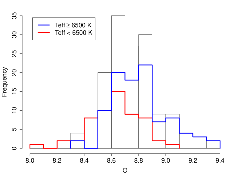
Figure 6.— O abundances for our program stars.

The abundances derived from the different lines agree well. Taking the [O i] line at 6300 Å  as a reference the [O/H] abundances derived from the other lines show a mean differences of $-0.07\pm 0.19\,\text{dex}$ (5577 Å), and $-0.05\pm 0.16\,\text{dex}$ (6363 Å), where the [O/H] abundances for each line are relative to the solar abundance derived with the same line. The O abundances of the triplet lines show larger differences for strong lines that suffer from saturation. We therefore consider only abundances derived from triplet lines with $\text{EWs}<200\,\text{m\AA}$. With this constraint the difference reduces to $0.00\pm 0.19\,\text{dex}$. The scatter in the abundances indicated by the standard deviation is due to the higher temperature sensitivity of the triplet lines. Adjusting the temperatures of the objects by $53\pm 136\,\text{K}$ would result in identical O abundances for both the 6300 Å  line and the O triplet.

The O abundances for stars with high rotational velocities were derived in a way similar to the derivation of the C abundances. The flux was integrated for all stars in the wavelength range around the O i triplet (7765 - 7780 Å). This region contains more relevant contribution from O absorption than the 6300 Å line. Then, a linear model was constructed from the stars with non-LTE corrected O abundances derived from the O triplet lines using the integrated flux and the atmospheric parameters, and used to predict the O abundances for the high rotation stars taking again the errors in the O abundances as weights. The mean residual of this model is $0.01\pm 0.09$ dex. The error for the O abundances derived in this way is 0.17 dex. The calculated abundances for the high rotation stars are displayed in Table 9 and a histogram of the distribution of the O abundances is shown in Figure 6. As for C the high rotators, with their higher metallicities, show slightly higher O abundances.

In Figure 7 the derived O abundances are compared with the results from Luck & Heiter (2006). They use a synthesis of the forbidden line at 6300 Å  as the sole indicator for the O abundance. While Luck & Heiter use the same ${\log gf}$ value for the O line as we do, the strength of the blending Ni line is determined under the assumption that [Ni/Fe] = 0 with the experimental ${\log gf}$ value from Johansson et al. (2003).

Overall, the distribution of O abundances at a given [Fe/H] are slightly more dispersed than the C abundances. Luck & Heiter attributed the larger scatter of the O abundances compared to C partly to the difficulty of determining the O abundance from the weak [O i] line. The [O/H] abundances agree well despite the differences in the lines used for the analysis: a slight offset exists with our program stars being about 0.06 dex higher than the linear fit to Luck & Heiter’s data. Ecuvillon et al. (2006) derived O abundances for F-K stars including many hosting exoplanets. Their abundance indicators were the [O i] 6300 Å  lines, the O i 7774 Å  triplet and several ultraviolet OH lines. Luck & Heiter compared their O abundances for 48 stars in common with Ecuvillon et al. and found a mean difference of only -0.02 dex. RR Lyr (HIP 95497) shows an exceptional high O abundance that is much higher than found in previous determinations (see Section IV.3).

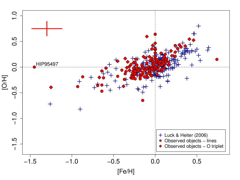
Figure 7.— Oxygen abundance relative to solar for our program stars. The cross indicates the typical error of the abundances derived with the individual lines.

IV.3. Comparison with literature values

Table 10Comparison of derived abundances of C, O, and Fe of our program stars with literature abundances. The rows with no source specified refer to our analysis. Asterisks mark mean values of pulsating stars.

object	${T_{\text{eff}}}$	${\log g}$	Fe	[Fe/H]	C	[C/H]	O	[O/H]	source
HIP 51056	7120	3.34	7.51		8.40		8.76		Rachkovskaya (2003)
	7206	3.54	7.61		8.29		8.80
HIP 64844	7300	3.20		0.45		-0.12		0.62	Galeev et al. (2012)
	7534	3.68		0.57		-0.46			Russell (1995)
	7361	2.97		0.74		-0.01		0.15
HIP 70602	7780	3.58	7.58				8.42		Takeda et al. (1999)
	7514	3.13	7.81				9.13
HIP 87998	6483	2.35	7.00		8.38		8.58		Adelman et al. (2008)
	6575	2.30	7.10		8.14		8.56		Luck & Wepfer (1995)
	7111	3.66	7.46		8.22		8.70
HIP 95497	6125	2.40		-1.57	7.16		8.02		Kolenberg et al. (2010)
	6622	2.31		-1.32			7.83		*Takeda et al. (2006)
	6304	3.04		-1.45	6.88		8.72
HIP 96302	5300	2.80		0.10		-0.18		-0.22	Balega et al. (2008)
	5132	3.04		-0.26		-0.44		-0.02
HIP 97985	5450	1.79		-0.67		-0.22			Takeda, Sato, & Murata (2008)
	5875	2.00	7.10		8.50		8.90		Vanture & Wallerstein (1999)
	5407	2.19	6.63	-0.87	8.21	-0.20	8.47
HIP 104185	6245	2.43		0.08		-0.19		0.05	*Takeda et al. (2013)
	6170	2.35		0.10		-0.05		0.05	Luck et al. (2008)
	6267	2.43		0.11		-0.12		0.01	Andrievsky et al. (2002)
	6155	1.42		0.02		-0.36		-0.14

Few of our stars have been previously analyzed. Table 10 shows a comparison of the published abundances. Naturally, this suffers from different techniques and data used. We therefore directly quote the parameters and abundances as presented by the authors. In general literature and newly determined abundances agree within the uncertainties of the determination. However, there are some noteworthy discrepancies.

The most significant deviation is the O abundance of RR Lyr (HIP 95497). Kolenberg et al. (2010) derived an O abundance of 8.02 by spectral synthesis of 6 O features. Their result agrees well with Takeda et al. (2006), who determined an O abundances of 7.96 by synthesizing the wavelength regions of 6154.5 - 6159.5Å  and 7770-7777Å. Both quoted O abundances are the mean of the abundances derived for several pulsation phases. Due to the blending of telluric O₂ lines, Takeda et al. made use of the [O i] forbidden line in only one case, for which they measured an EW of 3.9 mÅ  (O = 7.76). This compares to an EW of 23.5 mÅ  in our spectra (O = 8.97). The difference in the measured EWs might suggest a residual telluric component in our O line but all lines were carefully de-blended when the EWs were measured. The non-LTE corrected O abundance derived by the O triplet in our spectra is 8.64 a value in agreement with the [O i] line but higher than the one determined by Takeda et al. Despite the differences in the determined abundances it is interesting that HIP 95497 appears in the sample at all. The prototype of the RR Lyrae stars is a horizontal branch object and has therefore already experienced a first ascent of the giant branch. Unfortunately, with the given target selection and analysis method it is not possible to distinguish horizontal branch stars from late MS and subgiant stars.

For HIP 104185 the derived ${\log g}$ is lower than in previous determinations. This leads to both lower abundances in O and C.

For HIP 97985 there appears to be a larger difference between our O abundance and the one determined by Vanture & Wallerstein (1999). They derived their O abundance with measured EWs for the O triplet. The abundances were corrected for NLTE effects with the prescription of Eriksson & Toft (1979). The difference in ${T_{\text{eff}}}$ between ours and the determination of Vanture et al. might account for the major part of the difference. Raising our ${T_{\text{eff}}}$ by 400 K would lead to O = 8.71.

IV.4. Outliers

To get a quantitative estimate of the divergence in C abundances of the program stars in Figure 5, the difference between [C/H] of each star and the assumed offset of -0.1 dex from the trend of Luck & Heiter (2006) was determined (see Section IV.1), i.e. how much the [C/H] abundances diverge from the dashed line in Figure 5. To account for the uncertainty in the abundance determination these differences $\Delta$[C/H] were multiplied with a random value of the order of the mean error in [C/H]. This increases the scatter in the distribution of $\Delta$[C/H] and helps to detect if the distribution of outliers is in agreement with the observational scatter. A histogram of $\Delta$[C/H] can be seen in Figure 8. It shows that the distribution is centered on zero, as expected, and falls off steeply. The [C/H] abundances of most stars in the sample are therefore in accordance with the observational scatter about the expected trend with [Fe/H].

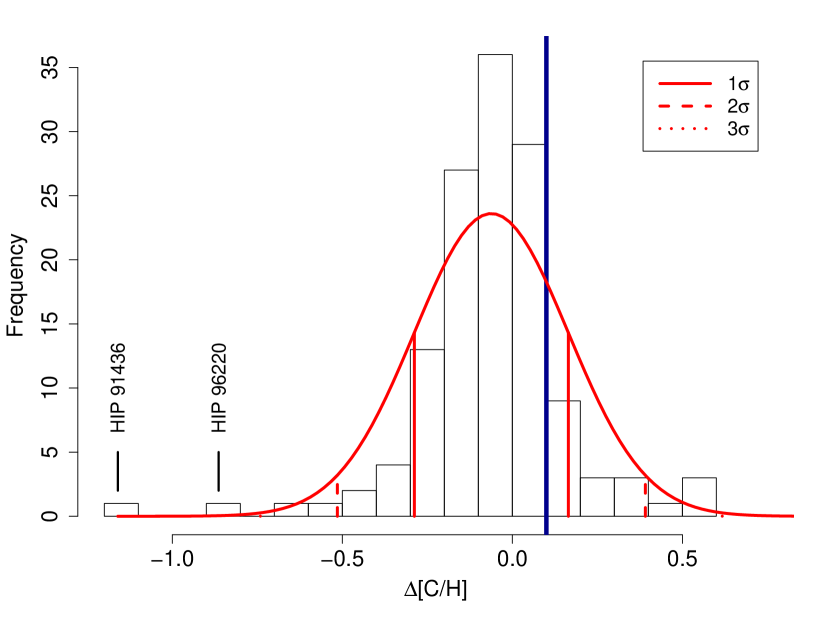
Figure 8.— Histogram of differences in [C/H] from assumed offset of -0.1 dex from Luck & Heiter (2006). The vertical line indicates the trend of Luck & Heiter.

However, two objects show a $\Delta\text{[C/H]}$ larger than $3\,\sigma$, HIP 91436 and HIP 96220. Both stars belong to the class of the Am and Ap stars. Abundance peculiarities for Am and Ap stars are well known and usually appear in the form of enhanced abundances of heavy metals and lower abundances of elements like Ca or Sc. A search through the most extensive catalogue of Am, Ap, and HgMn stars by Renson & Manfroid (2009) revealed that 28 stars in our sample have previously been identified as Am or Ap stars including the majority of stars with low C abundances. In Figure 9 only the Am or Ap stars in the sample are plotted and compared to C determinations for a sample of Am and Ap stars from Fossati et al. (2007) and Roby & Lambert (1990). For the objects in Roby & Lambert no metallicities were provided by the authors and the values for [Fe/H] in Figure 9 were taken from other literature sources. The underabundances in C for their objects are of comparable magnitude as the ones found for the Am/Ap stars among the observed objects. In addition to the C deficiency, the literature abundances generally show a deficiency in O that is not apparent in our Am/Ap sample (compare Figure 7). The comparison with Figure 5 and 8 also shows that the Am/Ap stars account for all stars with low [C/H] and $\Delta$[C/H]$>2\,\sigma$.

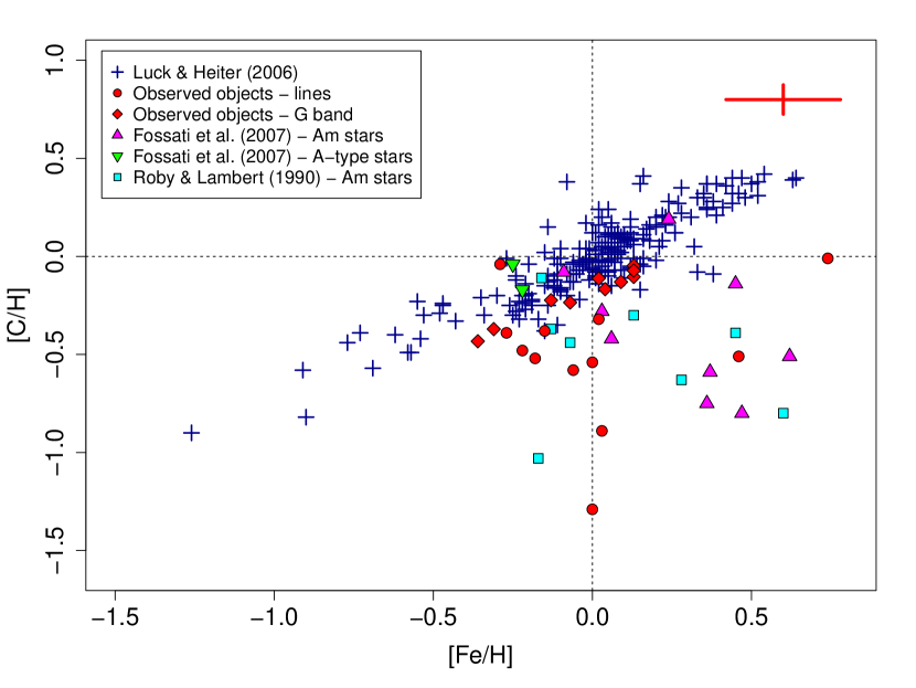
Figure 9.— C abundances of Am/Ap stars in the sample compared with literature values of a different set of Am/Ap stars and normal stars.

V. Discussion

Our analysis of a large sample of stars between 2 – 5 $M_{\odot}$ in the Hertzsprung gap shows that the abundances of C and O are generally consistent with those of normal mass dwarf stars and that no significant alteration of these elements can be found before the atmosphere is homogenized by the first dredge-up and abundance changes for light nuclides are introduced as material exposed to mild H-burning is mixed into the deep convective envelope. Before the dredge-up the abundances of C and O are stable during the evolution through the Hertzsprung gap. This is evident by the constant C/O ratio during this period that shows no dependency on ${T_{\text{eff}}}$   as can be seen in Figure 10.

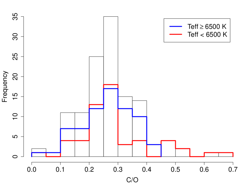
Figure 10.— C/O abundances for our program stars.

The fact that no difference in the C/O ratio can be found between stars located on the two sides of the Hertzsprung gap indicates that any rotationally induced mixing that might be present in stars with high rotational velocities at the blue side of the Hertzsprung gap is not strong enough to have an effect on the relative abundances of C and O in these stars. In fact, the only abundance anomalies in the sample are apparent for the slow rotating Am/Ap stars. As noted above, the Am and Ap stars generally exhibit a C deficiency. This abundance anomaly and the other numerous anomalies found in other Am/Ap stars are widely attributed to diffusive separation in the outer envelope of the star resulting from competition between gravitational settling and radiative levitation (Michaud 1970). Successful diffusive separation requires slow rotation rates to suppress rotationally-induced mixing and this explains why the majority of slow rotators among A-type main sequence stars are chemically peculiar (Abt 2009). In terms of the light elements, the C, N, and O abundances found by Fossati et al. (2007) can be reproduced well by the theoretical realization of diffusive separation by Richer, Michaud, & Turcotte (2000). Since the Am and Ap abundance anomalies result from a redistribution of an element within the envelope including the atmosphere, the redistribution is canceled by the deep convective envelope that constitutes the first dredge-up. In the models of Richer et al. (2000) the strength of the abundance anomaly in the atmosphere is controlled by the depth of the zone mixed by turbulence. For the observed abundance anomalies of the Am/Ap stars the central regions of the star are not mixed significantly. That suggests that the mechanism used to explain the Am/Ap star abundances can not be responsible for the C deficiency found in the peculiar wk Gb stars that require that CN-cycled material was processed at temperatures of 20 million degrees or hotter in the interior of the star (Adamczak & Lambert 2013, see Figure 11). For these objects rotation rates even higher than observed for the stars in the present sample might be required to induce mixing that extends into interior regions where some H-burning occurs and to connect these regions with the surface. Some rapidly-rotating stars might then be C-poor and N-rich. A search for such stars will be challenging but realizable (Lambert, McKinley, & Roby 1986).

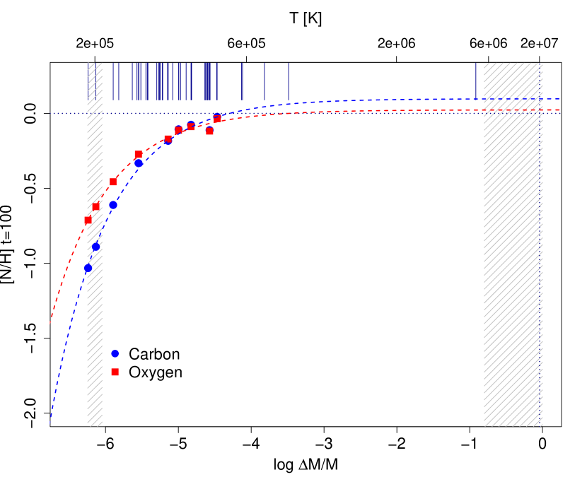
Figure 11.— Surface abundance for C and O for a 2.5 $M_{\odot}$ model vs. depths of turbulent mixing. Dashed regions mark convection zones below the surface and in the core. Vertical lines at the top of the plot mark mixing depths of all turbulence models presented in Richer et al. (2000).

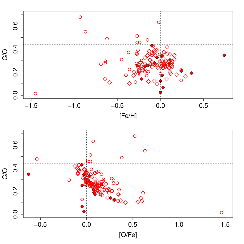
Figure 12.— C/O ratio for our program stars vs. [Fe/H] (top panel) and [O/Fe] (bottom panel). The symbol shapes are the same as in Figures 5 and 7, filled symbols mark the Am/Ap stars in the sample.

Apart from the peculiar stars in the sample, the abundances of the stars in the Hertzsprung gap follow the systematics found for normal mass stars. Furthermore, the abundances of all stars are in accordance with the Galactic chemical evolution. There is a trend between the C/O ratio and the [O/Fe] abundance of the stars in our sample and the stars with low metallicities tend to have higher [O/Fe] (see bottom panel of Figure 12). Gustafsson et al. (1999) found a trend between the C/O ratio and [Fe/H] for late F and early G type dwarfs in the Galactic Disk that they attributed to the metallicity dependence of the yields of C production in massive stars and the difference in time scale between the C production in less massive stars and the O production in massive stars. We can not confirm such a trend for the stars in our sample. There is evidence that the stars in the Hertzsprung gap are in agreement with a rather constant relation between C/O and [Fe/H]. This includes the Am/Ap stars that can not be clearly distinguished from the rest of the sample (cf. top panel in Figure 12). The local dwarfs from Luck & Heiter (2006) show a similar behavior and scatter with no certain trend. Compared to their objects, however, the C/O ratio for most of the program stars is subsolar. This is a reflection of the slightly lower C abundances obtained by our abundance analysis (see Section IV.1).

VI. Concluding Remarks

Our C and O abundance analysis of a large sample of stars in the Hertzsprung gap allows to draw a picture of the characteristics of stars in the mass range 2 – 5 $M_{\odot}$ in their evolution from the main sequence to the giant branch. Apart from the chemical peculiarities of the Am/Ap stars that are formed in their main sequence phase and are erased by the first dredge-up as the stars ascend the giant branch, it appears that no other abundance anomalies are surfacing during this evolutionary state and that the abundances of basic elements like C and O are not noticeably altered during the transition of the gap before the dredge-up.

The abundances determined for the program stars are in agreement with the those of local lower mass dwarf stars and follow the trends that are expected from Galactic chemical evolution. No clear indication of severe rotationally-induced mixing in the fast rotating stars of the sample could be found, however, we are limited here by the methods applied and an extension of the abundance analysis towards higher rotation rates might be worthwhile.

References

- Abt (2009) Abt, H. A. 2009, AJ, 138, 28
- Abt & Morrell (1995) Abt, H. A. & Morrell, N. I. 1995, ApJS, 99, 135
- Adamczak & Lambert (2013) Adamczak, J. & Lambert, D. L. 2013, ApJ, 765, 155
- Adelman, Cay, Tektunali, Gulliver, & Teker (2008) Adelman, S. J., Cay, I. H., Tektunali, H. G., Gulliver, A. F., & Teker, A. 2008, Astronomische Nachrichten, 329, 4
- Allende Prieto, Lambert, & Asplund (2001) Allende Prieto, C., Lambert, D. L., & Asplund, M. 2001, ApJ, 556, L63
- Alonso, Arribas, & Martínez-Roger (1999) Alonso, A., Arribas, S., & Martínez-Roger, C. 1999, A&AS, 140, 261
- Andrievsky, Kovtyukh, Luck, Lépine, Bersier, Maciel, Barbuy, Klochkova, Panchuk, & Karpischek (2002) Andrievsky, S. M., Kovtyukh, V. V., Luck, R. E., Lépine, J. R. D., Bersier, D., Maciel, W. J., Barbuy, B., Klochkova, V. G., et al. 2002, A&A, 381, 32
- Asplund, Grevesse, Sauval, Allende Prieto, & Blomme (2005) Asplund, M., Grevesse, N., Sauval, A. J., Allende Prieto, C., & Blomme, R. 2005, A&A, 431, 693
- Asplund, Grevesse, Sauval, Allende Prieto, & Kiselman (2004) Asplund, M., Grevesse, N., Sauval, A. J., Allende Prieto, C., & Kiselman, D. 2004, A&A, 417, 751
- Asplund, Grevesse, Sauval, & Scott (2009) Asplund, M., Grevesse, N., Sauval, A. J., & Scott, P. 2009, ARA&A, 47, 481
- Balega, Leushin, Kuznetsov, & Tamazian (2008) Balega, Y. Y., Leushin, V. V., Kuznetsov, M. K., & Tamazian, V. 2008, Astronomy Reports, 52, 226
- Barklem, Stempels, Allende Prieto, Kochukhov, Piskunov, & O’Mara (2002) Barklem, P. S., Stempels, H. C., Allende Prieto, C., Kochukhov, O. P., Piskunov, N., & O’Mara, B. J. 2002, A&A, 385, 951
- Bernacca & Perinotto (1970) Bernacca, P. L. & Perinotto, M. 1970, Contributions dell’Osservatorio Astrofisica dell’Universita di Padova in Asiago, 239, 1
- Bertelli, Girardi, Marigo, & Nasi (2008) Bertelli, G., Girardi, L., Marigo, P., & Nasi, E. 2008, A&A, 484, 815
- Bertelli, Nasi, Girardi, & Marigo (2009) Bertelli, G., Nasi, E., Girardi, L., & Marigo, P. 2009, A&A, 508, 355
- Bidelman (1951) Bidelman, W. P. 1951, ApJ, 113, 304
- Cameron & Fowler (1971) Cameron, A. G. W. & Fowler, W. A. 1971, ApJ, 164, 111
- Carquillat & Prieur (2007) Carquillat, J.-M. & Prieur, J.-L. 2007, MNRAS, 380, 1064
- Castelli & Kurucz (2004) Castelli, F. & Kurucz, R. L. 2004, Modeling of Stellar Atmospheres (IAU Symp. No. 210), ed. N. Piskunov, W. Weiss, & D. Gray, 2003, poster A20 (arXiv:astro-ph/0405087)
- Cottrell & Norris (1978) Cottrell, P. L. & Norris, J. 1978, ApJ, 221, 893
- de Laverny, do Nascimento, Lèbre, & De Medeiros (2003) de Laverny, P., do Nascimento, Jr., J. D., Lèbre, A., & De Medeiros, J. R. 2003, A&A, 410, 937
- Demarque, Woo, Kim, & Yi (2004) Demarque, P., Woo, J.-H., Kim, Y.-C., & Yi, S. K. 2004, ApJS, 155, 667
- Ecuvillon, Israelian, Santos, Mayor, Villar, & Bihain (2004) Ecuvillon, A., Israelian, G., Santos, N. C., Mayor, M., Villar, V., & Bihain, G. 2004, A&A, 426, 619
- Ecuvillon, Israelian, Santos, Shchukina, Mayor, & Rebolo (2006) Ecuvillon, A., Israelian, G., Santos, N. C., Shchukina, N. G., Mayor, M., & Rebolo, R. 2006, A&A, 445, 633
- Eriksson & Toft (1979) Eriksson, K. & Toft, S. C. 1979, A&A, 71, 178
- ESA (1997) ESA. 1997, VizieR Online Data Catalog, 1239, 0
- Fossati, Bagnulo, Monier, Khan, Kochukhov, Landstreet, Wade, & Weiss (2007) Fossati, L., Bagnulo, S., Monier, R., Khan, S. A., Kochukhov, O., Landstreet, J., Wade, G., & Weiss, W. 2007, A&A, 476, 911
- Galeev, Ivanova, Shimansky, & Bikmaev (2012) Galeev, A. I., Ivanova, D. V., Shimansky, V. V., & Bikmaev, I. F. 2012, Astronomy Reports, 56, 850
- Gustafsson, Karlsson, Olsson, Edvardsson, & Ryde (1999) Gustafsson, B., Karlsson, T., Olsson, E., Edvardsson, B., & Ryde, N. 1999, A&A, 342, 426
- Hakkila, Myers, Stidham, & Hartmann (1997) Hakkila, J., Myers, J. M., Stidham, B. J., & Hartmann, D. H. 1997, AJ, 114, 2043
- Hiltgen (1996) Hiltgen, D. D. 1996, PhD thesis, PhD thesis, Univ. Texas Austin. (1996)
- Johansson, Litzén, Lundberg, & Zhang (2003) Johansson, S., Litzén, U., Lundberg, H., & Zhang, Z. 2003, ApJ, 584, L107
- Kolenberg, Fossati, Shulyak, Pikall, Barnes, Kochukhov, & Tsymbal (2010) Kolenberg, K., Fossati, L., Shulyak, D., Pikall, H., Barnes, T. G., Kochukhov, O., & Tsymbal, V. 2010, A&A, 519, A64
- Koleva, Prugniel, Bouchard, & Wu (2009) Koleva, M., Prugniel, P., Bouchard, A., & Wu, Y. 2009, A&A, 501, 1269
- Kraft (1967) Kraft, R. P. 1967, ApJ, 150, 551
- Kurucz, Furenlid, Brault, & Testerman (1984) Kurucz, R. L., Furenlid, I., Brault, J., & Testerman, L. 1984, Solar flux atlas from 296 to 1300 nm
- Lambert, McKinley, & Roby (1986) Lambert, D. L., McKinley, L. K., & Roby, S. W. 1986, PASP, 98, 927
- Lambert & Sawyer (1984) Lambert, D. L. & Sawyer, S. R. 1984, ApJ, 283, 192
- Lind, Bergemann, & Asplund (2012) Lind, K., Bergemann, M., & Asplund, M. 2012, MNRAS, 427, 50
- Luck, Andrievsky, Fokin, & Kovtyukh (2008) Luck, R. E., Andrievsky, S. M., Fokin, A., & Kovtyukh, V. V. 2008, AJ, 136, 98
- Luck & Heiter (2006) Luck, R. E. & Heiter, U. 2006, AJ, 131, 3069
- Luck & Heiter (2007) —. 2007, AJ, 133, 2464
- Luck & Wepfer (1995) Luck, R. E. & Wepfer, G. G. 1995, AJ, 110, 2425
- Massarotti, Latham, Stefanik, & Fogel (2008) Massarotti, A., Latham, D. W., Stefanik, R. P., & Fogel, J. 2008, AJ, 135, 209
- Mermilliod, Mermilliod, & Hauck (1997) Mermilliod, J.-C., Mermilliod, M., & Hauck, B. 1997, A&AS, 124, 349
- Michaud (1970) Michaud, G. 1970, ApJ, 160, 641
- Michaud (1977) —. 1977, Nature, 266, 433
- Palacios, Parthasarathy, Bharat Kumar, & Jasniewicz (2012) Palacios, A., Parthasarathy, M., Bharat Kumar, Y., & Jasniewicz, G. 2012, A&A, 538, A68
- Prugniel & Soubiran (2001) Prugniel, P. & Soubiran, C. 2001, VizieR Online Data Catalog, 3218, 0
- Prugniel, Vauglin, I., & Koleva (2011) Prugniel, P., Vauglin, I., & Koleva, M. 2011, VizieR Online Data Catalog, 353, 19165
- Przybilla, Butler, & Kudritzki (2001) Przybilla, N., Butler, K., & Kudritzki, R. P. 2001, A&A, 379, 936
- Rachkovskaya (2003) Rachkovskaya, T. M. 2003, Astronomy Reports, 47, 865
- Ramírez & Allende Prieto (2011) Ramírez, I. & Allende Prieto, C. 2011, ApJ, 743, 135
- Ramírez, Allende Prieto, & Lambert (2007) Ramírez, I., Allende Prieto, C., & Lambert, D. L. 2007, A&A, 465, 271
- Ramírez & Meléndez (2005) Ramírez, I. & Meléndez, J. 2005, ApJ, 626, 465
- Renson & Manfroid (2009) Renson, P. & Manfroid, J. 2009, A&A, 498, 961
- Richard, Michaud, & Richer (2001) Richard, O., Michaud, G., & Richer, J. 2001, ApJ, 558, 377
- Richard, Michaud, Richer, Turcotte, Turck-Chièze, & VandenBerg (2002) Richard, O., Michaud, G., Richer, J., Turcotte, S., Turck-Chièze, S., & VandenBerg, D. A. 2002, ApJ, 568, 979
- Richer, Michaud, & Turcotte (2000) Richer, J., Michaud, G., & Turcotte, S. 2000, ApJ, 529, 338
- Roby & Lambert (1990) Roby, S. W. & Lambert, D. L. 1990, ApJS, 73, 67
- Royer, Grenier, Baylac, Gómez, & Zorec (2002) Royer, F., Grenier, S., Baylac, M.-O., Gómez, A. E., & Zorec, J. 2002, A&A, 393, 897
- Russell (1995) Russell, S. C. 1995, ApJ, 451, 747
- Saffe (2011) Saffe, C. 2011, rmxaa, 47, 3
- Schröder, Reiners, & Schmitt (2009) Schröder, C., Reiners, A., & Schmitt, J. H. M. M. 2009, A&A, 493, 1099
- Sneden, Lambert, Tomkin, & Peterson (1978) Sneden, C., Lambert, D. L., Tomkin, J., & Peterson, R. C. 1978, ApJ, 222, 585
- Sneden (1973) Sneden, C. A. 1973, PhD thesis, The University of Texas at Austin.
- Takeda, Honda, Aoki, Takada-Hidai, Zhao, Chen, & Shi (2006) Takeda, Y., Honda, S., Aoki, W., Takada-Hidai, M., Zhao, G., Chen, Y.-Q., & Shi, J.-R. 2006, PASJ, 58, 389
- Takeda, Kang, Han, Lee, & Kim (2013) Takeda, Y., Kang, D.-I., Han, I., Lee, B.-C., & Kim, K.-M. 2013, MNRAS, 432, 769
- Takeda, Sato, & Murata (2008) Takeda, Y., Sato, B., & Murata, D. 2008, PASJ, 60, 781
- Takeda, Takada-Hidai, Jugaku, Sakaue, & Sadakane (1999) Takeda, Y., Takada-Hidai, M., Jugaku, J., Sakaue, A., & Sadakane, K. 1999, PASJ, 51, 961
- Tomkin, Sneden, & Cottrell (1984) Tomkin, J., Sneden, C., & Cottrell, P. L. 1984, PASP, 96, 609
- Tull, MacQueen, Sneden, & Lambert (1995) Tull, R. G., MacQueen, P. J., Sneden, C., & Lambert, D. L. 1995, PASP, 107, 251
- van Leeuwen (2007) van Leeuwen, F. 2007, A&A, 474, 653
- Vanture & Wallerstein (1999) Vanture, A. D. & Wallerstein, G. 1999, PASP, 111, 84
- Wallerstein, Böhm-Vitense, Vanture, & Gonzalez (1994) Wallerstein, G., Böhm-Vitense, E., Vanture, A. D., & Gonzalez, G. 1994, AJ, 107, 2211
- Wu, Singh, Prugniel, Gupta, & Koleva (2011) Wu, Y., Singh, H. P., Prugniel, P., Gupta, R., & Koleva, M. 2011, A&A, 525, A71