On-sky performance during verification and commissioning of the Gemini Planet Imager’s adaptive optics system

Abstract

The Gemini Planet Imager instrument’s adaptive optics (AO) subsystem was designed specifically to facilitate high-contrast imaging. It features several new technologies, including computationally efficient wavefront reconstruction with the Fourier transform, modal gain optimization every 8 seconds, and the spatially filtered wavefront sensor. It also uses a Linear-Quadratic-Gaussian (LQG) controller (aka Kalman filter) for both pointing and focus. We present on-sky performance results from verification and commissioning runs from December 2013 through May 2014. The efficient reconstruction and modal gain optimization are working as designed. The LQG controllers effectively notch out vibrations. The spatial filter can remove aliases, but we typically use it oversized by about 60% due to stability problems.

1 INTRODUCTION

The Gemini Planet Imager (GPI) [1] is a hyper-spectral coronagraphic instrument specifically designed to directly image exoplanets. GPI and the SPHERE instrument [2] are part of a new generation of instruments that feature specialized adaptive optics (AO) systems that use thousands of actuators and specialized algorithms. In this paper we discuss the algorithms and technologies that were developed for GPI, and how well they are actually working during the instrument’s verification and commissioning period at Gemini South (late 2013-summer 2014).

2 Experimental procedures and data analysis

The performance of the AO system is analyzed primarily through system diagnostic data. This telemetry is dumped at the full frame rate of the AO system and can include anything from raw CCD frames, to calculated centroids, to reconstructed phases to deformable mirror commands. By synchronizing multiple data dumps, long streams of telemetry can be saved during on-sky experiments. During a typical on-sky experiment, 22-second streams of telemetry are saved. The specific control parameters in use (e.g. filter coefficients) are also saved. These data are analyzed offline using a standard telemetry analysis code.

Our primary analysis technique is to examine the temporal power spectral densities (PSDs) of specific modes that the system controls. For tip, tilt and focus we analyze the coefficients directly. For the higher order phase, we begin with the residual phase as seen by the AO system directly after phase reconstruction from the centroids. For a given 22-second interval, the $x$-$y$-$t$ data cube is converted at each time step into the frequency domain to produce a $f_{x}$-$f_{y}$-t data cube. Given the time series of a modal coefficient (e.g. tip, Fourier mode $k=12$, $l=12$, where $k$ and $l$ indicate the index into a $48\times 48$ FFT of the phase), the temporal PSD is estimated by the averaged modified periodogram technique [3].

This temporal PSD represents what is measured by the AO system in closed loop. For bright targets wavefront sensor (WFS) noise is small and this is very close to the closed-loop error that should be presented at the output of the AO system to the science leg. On moderate and dim targets, however, the measurement and the error are not the same. To analyze the error, as opposed to the measurement, we use the exact same technique that the gain optimizer (see below) uses [4]. To estimate the error, we take the temporal PSD of the measurement and invert by the known system response. This is possible because the temporal response of the system is very well characterized. As shown in Figure 1, the temporal behavior for focus and a Fourier mode both closely follow our models.

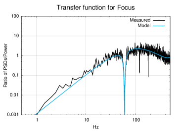
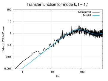
Figure 1: The temporal performance of the AO system is well-characterized; measured error transfer functions using the internal source agree with models. For [left] focus and [right] a low-order Fourier mode, the measured response on the internal source is given in black, and the model in blue. Telemetry: _When_2014.5.9_18.54.42

Once the PSD of the closed-loop measurement is converted into the PSD of the estimated open-loop measurements, we then split it into signal and noise components. The noise component should be temporally white, and it is estimated by taking a median of the PSD at the highest frequencies. This estimate is the PSD of the input noise seen by the AO system. The PSD of the signal (primarily atmosphere) seen by the AO system is obtained by subtracting the noise PSD from the estimated open-loop measurement PSD. We now have estimated temporal PSDs for the signal that the AO system wants to correct and the WFS noise that it measures. The error produced by the AO system is estimated by apply the error transfer function (ETF) to the signal PSD and the noise transfer function (NTF) to the noise PSD. This frequency domain method ignores any static level of error, which is removed before the periodogram calculation. As such (see Section 8) this term is calculated separately. Note that throughout this paper we rely on the self-reporting of the AO system for performance analysis. A provisional error budget is given in Section 8, but a rigorous comparison of science measurements to AO telemetry is beyond the scope of this present work, but will be included in a future publication.

3 Fourier transform reconstruction

3.1 Technology description and methods

The concept of reconstructing the wavefront phase from slopes with a filtering approach was originally proposed in the mid 1980s [5, 6]. However, the boundary problem imposed by a circular (or annular) aperture in the square computational grid prevented the method from practical use. By solving this boundary problem, we were able to make the filtering approach feasible, calling the method Fourier Transform Reconstruction (FTR) [7]. We further defined new filters that better captured Shack-Hartmann behavior [8, 4] and showed that the Fourier basis provided a tight frame for modal control [4]. When formulated to consider the signal and noise power levels, the FTR method is a Wiener filter [9], and we showed that FTR is equivalent [9] to the Minimum Variance Unbiased approach [10] if the Fourier basis set is used. To our knowledge, the use of FTR in GPI represents the first on-sky use of a computationally efficient wavefront reconstruction method (as opposed to a parallelized vector-matrix-multiply) in an astronomical AO system.

After phase reconstruction the residual is split [11] between two deformable mirrors (DMs). Low-spatial-frequency Fourier modes, which require the most stroke, are sent to the “Woofer” DM, a conventional piezo DM manufactured by Cilas. The high-order phase is sent to the “Tweeter” DM, a microelectromechanical systems (MEMS) mirror developed by Boston Micromachines.

3.2 On-sky results

Use of FTR was motivated by computational complexity; a matrix multiplication of a system of the same size would require 45 times more computation. This enabled the implementation of the real-time controller (RTC) on a commercial, off-the-shelf (COTS) server running real-time linux, as opposed to customized or special-purpose hardware such as digital signal processors (DSPs) or graphics processing units (GPUs). As we see below, the use of FTR makes the residual Fourier coefficients of the wavefront available, which facilitates computationally efficient controller optimization. As of May 2014, the total delay from the end of a WFS frame integration to the application of the phase commands on the DMs is 1.7 msec. This is true for either 1 kHz or 500 Hz operation. The tip, tilt and focus commands are computed more quickly since they do not go through the FTR process. Those commands are placed on the Woofer DM and the tip-tilt stage after 1.2 msec. For both of these with first 890 microsec are taken up by the detector read.

As has been noted by us elsewhere[12], use of FTR requires precise alignment of the AO system optics. This alignment is achieved through automatic processes before each acquisition [13]. The rotation of the spots grid produced by the lenslets relative to the WFS CCD pixel grid has proved problematic. As was originally noted in Section 5.2 of our prior work [12], if rotation exists in the centroids, it will be reconstructed by FTR into a shape that has a scalloping pattern around the edges. During closed-loop operation this behaves similarly to an alias - a non-physical signal is present in the slopes and makes it through to the DM, where a shape builds up to attempt to correct it.

As built, there is a small but not insignificant amount of rotation in the WFS, which is nominally included in the reference slopes. The removal of rotation via reference subtraction will not work completely if some effect changes the gain of the quad cells. This could be a drift of the bias level on the CCD [14], spot size variations due to atmospheric turbulence, or potentially other subtle factors. During integration and testing we identified that bias drift was significantly reducing performance quality; the short-term solution was taking regular dark frames. Despite regular darks, during the December run we identified that rotation was not being fully removed on-sky, most likely due to spot size variations that are dependent on seeing. These spot size variations result in a large status excursion of the Tweeter actuators from flat around the edges of the pupil. To solve this problem the RTC now includes a step where rotation is explicitly removed from the centroids before FTR. This approach has been verified to work correctly, and has reduced the edge excursions. Pending results from other analysis by Greenbaum [15] and Sadakuni [14] the specific vectors used in the removal process may be modified.

This is our best solution to date for this problem with FTR. On a symmetric pupil this effect is entirely due to the edge correction process where the slopes on the square grid are managed. An equivalent matrix reconstructor on a symmetric pupil would not let any rotation through. As a further complication, GPI does not have a symmetric pupil; small subregions are masked off to prevent the AO system from seeing the dead actuators, which are mostly positioned at the exterior edge of the pupil. This asymmetry allows for rotation to leak through both FTR and a matrix reconstructor. If we were using a matrix method, we would not need to do the removal step from the centroids but could instead account for the rotation internally in the matrix.

4 Modal gain optimization

4.1 Technology description and methods

Originally proposed by Gendron and Lena [16], modal gain optimization is a technique where the wavefront phase is decomposed into orthogonal modes (as opposed to actuator positions in the pupil). Using either open- or closed-loop telemetry on-sky, the control loop gain of each mode is set such that it minimizes the residual error variance. Modal gain optimization has been implemented in several AO systems, including the initial demonstration in Come-On-Plus [17], which used open-loop telemetry prior to an observation. The method is used in the Altair AO system at Gemini North [18] and ESO’s NAOS system [19]. More recently, modal gain optimization for up to 400 modes has been implemented in the LBT’s FLAO system [20]. As described, that optimization is done once at the beginning of an observation, and proceeds iteratively.

In GPI, the modal gain optimization procedure operates continuously as a supervisory process. As described fully elsewhere [4], the Fourier coefficients of the residual phase are buffered during the reconstruction process. Each mode is analyzed temporally, using the averaged-modified periodogram technique to estimate the closed-loop power spectral density (PSD) of the measurements. Using a fast root-finding technique, the best modal gain for each Fourier mode is calculated independently. All 2304 modal gains (which have hermitian symmetry on the spatial frequency grid, so only half need to be calculated) are used in a gain filter which is applied during the reconstruction process. Because the Fourier modal coefficients are directly available in closed loop, and because changing the modal gains involves simply changing a 2304-element vector in memory, the Fourier framework of GPI allows modal gain optimization to be conducted every eight seconds for all 2304 Fourier modes during closed loop. As such, we consider GPI to be unique in terms of the large number of modes that it optimizes, and the fact that it does so continuously during science observations.

4.2 On-sky results

During the integration and testing phase, the modal gain optimization was verified through off-line re-analysis of telemetry. That is, our analysis codes estimated the modal gains from telemetry, and the results were compared to what the system itself had calculated. The primary concern of our on-sky testing is whether the modal gain optimizer improves overall AO performance. To test this, we conducted a series of experiments. For a given star magnitude and frame rate, we closed the AO loops with a fixed value of uniform modal gain. After taking telemetry we turn on the gain optimizer and let the gains settle, a process that takes less than 30 seconds. We then take another telemetry set. We repeat this uniform gain-optimized gain pairing several times, slowly stepping up the initial uniform gain from 0.05 to 0.3 with increments of 0.05. This gives us an interleaved set of measurements over a period of about 20 minutes, with six examples of uniform gain filters spanning the range of stable gains and six examples of optimized gains. During our March run we conducted four of these tests. Representative gain filters for the four cases are shown in Figure 2. As predicted by simulations [21], the gain filters span a wide range of possible gains, and show evidence of wind direction.

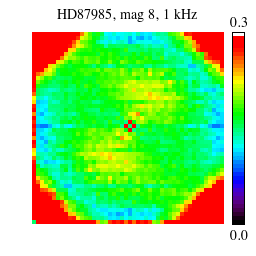
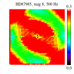
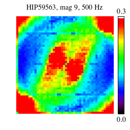
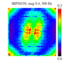
Figure 2: Modal gain filters as determined during closed-loop operation on sky. Each panel color scale goes from 0.0 to 0.3 for the gain. Piston ($k=0$, $l=0$) is at middle; waffle ($k=24$, $l=24$) is at the corner. Wind direction is visible, particular in the two cases at right. Telemetry sets: _When_2014.3.24_1.56.52, _When_2014.3.24_1.36.1, _When_2014.3.24_2.37.15 and _When_2014.3.24_3.3.31.

Using the methods described in Section 2, we estimate the error for each Fourier mode and for all modes together. Figure 3

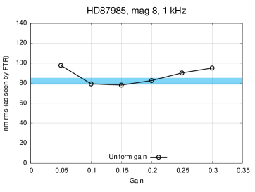
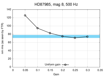
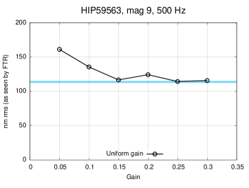
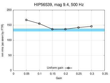
Figure 3: Error estimated from AO measurements, for three different targets for the optimizer test. In each case black points represent the six uniform gain trials; blue band represents full range of error for the six optimizer trials. Best performance on target HD87985 comes with optimization at 500 Hz, not at 1 kHz. Telemetry: 48 different telemetry sets used spanning the period _When_2014.3.24_1.25.48 to _When_2014.3.24_3.13.12.

shows the estimates of total error. For each of the six uniform gain cases, the total error is marked by the black points. This total error is the sum of the error due to signal (which decreases as gain is increased) and the error due to noise (which increases as gain is increased). Analysis of the two components (not shown) confirms that the system follows this expected behavior. In the figure the blue bar indicates the full range of the total error, as estimated from the six different optimized cases. In all these cases the performance with the optimizer on (in blue) is at or very close to the minimum when the gain is adjusted by hand.

This total error metric shown in Figure 3 is dominated by the optimizer’s performance at low spatial frequencies. This is because both atmospheric turbulence and the noise propagation from the Shack-Hartmann wavefront sensor produce more power at lower frequencies. To further verify that the modal gain optimization is working for all modes, we analyzed each mode individually. Figure 4 shows the test results for four different Fourier modes that are representative of the 2304 controllable modes.

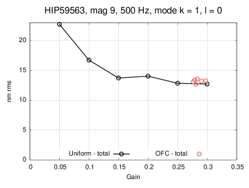
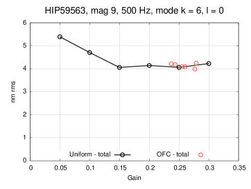
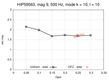
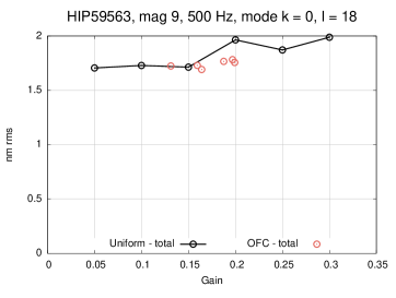
Figure 4: Estimated science-leg error from AO residuals, for four different Fourier modes (mode index given in plot titles). Black points are for the six uniform gain trials; red points are for the six optimized gain trials. Low-order modes (upper left) have a large amount of power, while higher-frequency modes have less. On a mode-by-mode basis the gain optimizer is correctly finding gains which minimize error. Telemetry: 12 different sets used spanning the period _When_2014.3.24_2.27.11 to _When_2014.3.24_2.47.5

As shown in this figure, for a 9th magnitude star at 500 Hz, the lowest spatial frequency modes (e.g. $k=1$, $l=0$ shown at upper left) have the most total error. In this case the atmosphere dominates and the optimizer correctly drives the modal gain to maximum. For mid-frequency modes, such as $k=6$, $l=0$ at upper right and $k=10$, $l=10$ at lower left, the atmosphere and noise are more equal. For these modes the optimizer uses a high, but not maximum gain. For the highest spatial frequencies, such as $k=0$, $l=18$ shown at bottom right, noise dominates and the optimizer drives the gain lower. These modes also have significant high-temporal frequency content due to aliasing (see below), which the optimizer does not explicitly know about.

In order to suppress waffle and reduce edge effects, during Integration and Test a modified Tweeter influence function filter was put in place. As discussed elsewhere [22], the estimated phase is pre-compensated by a influence function filter to correctly shape the phase on the Tweeter. Due to the broadness of the Tweeter influence function, the effective Tweeter gain for high spatial frequencies [23] is very small. Division by this small number inflates noise. As such, we artificially limit the division. As a result, the optimizer tends to drive up the gain on these under-compensated modes, as is obvious by the red regions in the corners of the gain filters shown in Figure 2. This behavior of the optimizer to correct for a miscalibration was discussed in Section 4.C of our original proposal [4]. It remains to be determined if artificially suppressing the influence function gains and then having the optimizer try to crank them back up is adversely affecting performance on-sky.

5 Spatially-filtered wavefront sensor

5.1 Technology description and methods

Aliasing occurs when a signal has frequency content above half of its sampling frequency. In an adaptive optics system, the atmosphere is not-band-limited; this will cause any sensor which samples the phase, either through lenslets or pixels, to measure spurious signals. These aliases will lead to extra residual error. Rigaut first calculated this as one-third of the classical fitting error [24]. PSD treatments such as those by Jolissaint [25] show that the exact amount of aliasing error depends on the filter type (derivative vs. direct phase) and the control parameters.

To prevent the aliasing error, we has proposed what we termed the spatially-filtered wavefront sensor (SFWFS) [26]. For a Shack-Hartmann sensor, this is implemented as a hard-edged field stop in a focal plane of the WFS before the lenslet array. In the case of a high-strehl system, the filter will reject phase errors that scatter light beyond the size of the field stop. In the case of a system with subaperture size $d$, the field stop with a diameter of $\lambda/d$ will reject content beyond the sampling limit, in theory producing a band-limited phase for the WFS to measure and producing a dark hole in the PSF. A first experimental demonstration of the SFWFS was done by Fusco [27], where as over-sized stop was shown to improve performance in a testbed with dynamic turbulence. In our own work we were able to demonstrate cleaning out a dark hole on static phase plate with a 32x32 MEMS mirror and sensor [28].

5.2 Modifications from original design

During the integration and testing phase of GPI, we had to make some accommodations in using the SFWFS. In particular we discovered that when sized to nominal (i.e. $\lambda/d$), we observed non-linear effects in edge sub-apertures and in the subapertures near the Tweeter’s dead actuators. Fourier optics simulations revealed that for large phase errors such as an actuator stuck more than a micron from its neighbors, the spatial filter is non-linear and will produce biased measurements. To mitigate this, we implemented a stronger leak (for an integral controller of the form $g/(1-c\mathrm{z}^{-1})$, $c$ would be set to 0.9) on the actuators immediately next to the dead actuators to bleed off this error. Another problem we encountered is poor stability at the edge of the pupil, which leads to loss of light. During integration and testing we examined this, and found it was exacerbated by a still poorly-understood effect on the partially illuminated subapertures along the outer edge of the pupil. During this phase we had also used a stronger leak ($c=0.9$) on the actuators bordering these partially-illuminated subapertures. During our May 2014 testing run we switched to simply not using measurements from these partially illuminated subapertures around the outside edge. Operation remains good in this slightly modified configuration, though it remains to be determined if this has improved spatial filter stability at all.

5.3 On-sky results

We can assess the ability of the SFWFS to reject specific spatial frequencies by examining the temporal PSDs of the Fourier modes during closed loop. When frozen flow is present (which it typically is), the wind motion creates characteristic peaks in the temporal PSDs of the Fourier modes. For any Fourier mode of spatial frequency (inverse-meters) $<f_{x},f_{y}>$ a wind layer with velocity vector (m/s) $<v_{x},v_{y}>$, a peak appears in the PSD at temporal frequency (Hz) $f_{x}v_{x}+f_{y}v_{y}$. For the controllable modes, this creates a characteristic pattern (see Figure 4 of Poyneer et al. [29]). When a spatial frequency above the sampling limit of the AO system is measured, it aliases down to a lower spatial frequency, but the temporal frequency of the wind component stays the same. This results in peaks in the controllable modes from aliasing at temporal frequencies $(f_{x}\pm d^{-1})v_{x}+(f_{y}\pm d^{-1})v_{y}$, where $d$ is the subaperture size in the pupil, e.g. 18 cm for GPI. An example of this is shown in Figure 5, left side.

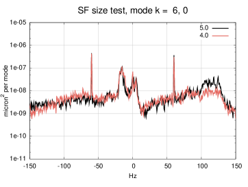
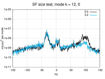
Figure 5: Bright star spatial filter test shows that the filter removes aliases of wind-blown turbulence. At left, the filter at 4.0 mm cleans up modes out to spatial frequency radius 6. At right, the filter at 3.2 mm cleans up modes out to spatial frequency radius 12. See text for a full explanation. Telemetry sets: _When_2014.5.14_19.53.43, _When_2014.5.14_19.58.46 and _When_2014.5.14_20.3.41 taken on target HD101615.

At left the plot shows that temporal PSD of the residual phase for Fourier mode $k=6$, $l=0$. We know, from examining the other Fourier modes, that the peak at -20 Hz is from frozen flow atmosphere. The alias is visible at right from 100 to 130 Hz. In black is the residual as seen with the SF = 5.0 mm. When the filter is closed to 4.0 mm, this alias is suppressed. (The leakage of the non-focus 60 Hz vibrations are clearly seen at 60 Hz for this Fourier mode). In the right panel we see Fourier mode $k=12$, $l=0$. In this case the wind peak has moved out to temporal frequency -30 Hz. The alias has moved down to about 90 to 110 Hz. For this higher frequency the blue curve shows the residual as seen with the SF at 3.2 mm. As the filter gets smaller, it cleans up aliases for controllable Fourier modes of higher frequency.

The figure shows data taken on May 14, 2014 on target HD101615. We also have data from December 11, 2013 on $\beta$ Pictoris down to SF size 2.8 mm. A qualitative analysis of the rejection of aliases of wind-blown turbulence produces estimates for the range of modes that the SFWFS “cleans up” by removing aliases. As given in Table 1, this follows the expected linear trend as a function of SF size. At size 3.2 mm, the filter cleans up modes to $k=12$, which is halfway out to the edge of the dark hole. Though as the filter narrows beyond this and more modes are cleared, overall performance is reduced due to edge effects that compromise stability. The $\beta$ Pictoris testing occurred during very good seeing (see first $\beta$ Pictoris column of  2). In this case we were able to stably close the filter to 2.8 mm, which we estimate clears out 66% of the dark hole. This performance is atypical.

Table 1: Estimates of spatial filter effectiveness for [left] 2013-12-11 on $\beta$ Pictoris and [right] 2014-5-14 on HD101615. The maximum spatial frequency for which the filter removes aliases is given; maximum possible value for $k$ is 24.

SF size (mm)	Spat. freq.
3.5	$k=10$
3.3	$k=11$
3.0	$k=14$
2.8	$k=16$

SF size (mm)	Spat. freq.
4.5	$k=0$
4.0	$k=6$
3.5	$k=10$
3.2	$k=12$

6 Tip-tilt vibration correction with LQG

6.1 Technology description and methods

Mathematical treatments of optimal control methods for AO date back more than a decade, such as Gavel & Wiberg’s [30] Kalman filter. Le Roux developed a Linear-Quadratic-Gaussian (LQG) framework for AO control[31], which was experimentally demonstrated in a testbed for vibration filtering by Petit [32]. Further progress has recently been made with an on-sky demonstration by Sivo of LQG for all modes in CANARY [33]. Another vibration scheme has been tested in GEMS by Guesalaga [34]. For use in GPI we have adapted the framework of Le Roux and added in the ability to work in a system with an arbitrary (i.e. non-integer frame) control delay [35], and also to correct both common-path and non-common-path vibrations [36], both of which were deemed necessary to use an LQG controller in GPI. As noted above, the tip-tilt and focus controllers have a 1.2 frame delay, which we account for explicitly in the LQG model.

6.2 Modifications from original design

There are two significant differences between the tip-tilt LQG filter as initially proposed and as used in GPI. First, in our proposal we presented a high-order model for the atmospheric tip-tilt; in practice we always use a first-order auto-regressive (AR(1)) model. Second, in GPI the pointing is actually controlled with two surfaces. By using a low-order low-pass filter, the low temporal frequency part of the pointing signal is sent to the high-stroke Stage, while the higher-frequency placed on the Woofer DM in combination with the phase correction. Since each mirror has its own integrator, the result of the LQG (which is integrated internally) must be converted to a pseudo-residual that is then split and integrated on each surface. Specifically, if the Woofer integrator has control law $C(\mathrm{z})=1/(1-0.999\mathrm{z}^{-1})$, the pseudo-residual is produced with a filter that is a“leaky” differentiator: $D(z)=1-0.999\mathrm{z}^{-1}$. We have had to be very conservative on the temporal split between the two surfaces to avoid instabilities; the current cutoff for the split is at 25 Hz. A more robust solution would have been to have the LQG model know explicitly about the temporal split [37].

6.3 On-sky results

During integration and testing we identified the pointing vibrations at 60, 120 and 180 Hz as the most significant. We were unable to determine if these tip-tilt vibrations are in the common path or the non-common path of the system, so we have assumed that they are common path and generated appropriate LQG filters. After analyzing on-sky telemetry with the default integral controllers for pointing, we generated LQG filters designed to recede the total vibration at 60, 120 and 180 Hz to 1 mas. LQG filters were tested in comparison to the default integral controller in an interleaved fashion. Pointing vibrations are always larger on the y-axis; in Figure 6

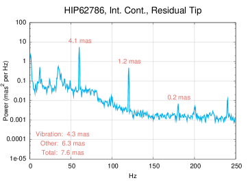
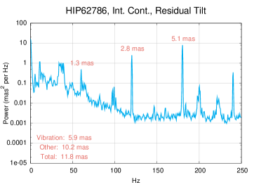
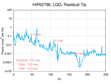
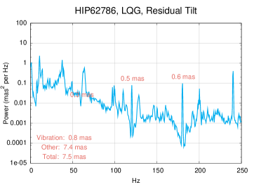
Figure 6: PSDs of closed-loop AO measurements for tip (left column) and tilt (right column), with estimated error amounts (red annotations). There are significant vibration-induced errors at 60, 120 and 180 Hz. With regular integral control (top row), these are 4 and 6 mas per axis. Use of a customized LQG controller (bottom row) reduces there vibration components to under 1 mas per axis. The same LQG model was used for both axes. Telemetry: _When_2014.5.12_19.50.22 and _When_2014.5.12_23.51.59.

we show the on-sky residual tip (top left) and tilt (top right) as seen by the WFS for the integral controller. At bottom is the results for our preferred LQG. The figure shows the AO measurements in closed loop. Annotated in red are the error levels (see Section 2 for a discussion of measurements versus error) passed on to science. The total vibration at 60, 120 and 180 Hz has been reduced to less than 1 mas for each axis with use of the LQG. The remaining pointing error is primarily residual atmosphere.

7 Focus vibration correction with LQG

7.1 Technology description and methods

When GPI is on the telescope, its cryocoolers cause vibration and result in significant phase errors. his manifests as a low-order wavefront - primarily focus, spherical and trefoil - with a temporal RMS of up to 150 nm occuring at 60 Hz. It remains unclear what is vibrating; either the secondary mirror moving in both piston and deforming, or a deformation of the primary mirror; both are very lightweight. For a thorough discussion of errors and mitigations, see Hartung [38]. This phase vibration was a highly suitable candidate for LQG correction - the error was highly concentrated at 60 Hz, and analysis of the temporal variation of the phase shape indicated that it was primarily focus that oscillated in total amplitude.

To correct this we simply applied the LQG filtering framework that had already been tested for tip-tilt. In the tip-tilt case, the signal is calculated and removed from the centroids and then sent to the LQG and on to the Stage and Woofer. In the case of focus we calculate focus directly from the slopes. To calculate and remove focus from the slopes via projection we use a model to make x- and y-slope vectors for focus. To apply the focus correction to the surface of the Woofer, we use the measured influence functions to generate a 9 by 9 signal which makes focus. The slope and command signals are calibrated against each other to ensure that the overall loop gain is 1.

7.2 On-sky results

The focus LQG was tested on-sky during the May run. In this case a pure focus shape was pulled out; the remaining components of the 60 Hz phase (mainly trefoil and spherical) were sent through the high-order loop. Figure 7 shows three different temporal PSDs of the focus measurements.

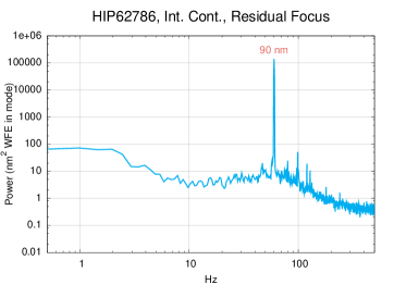
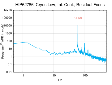
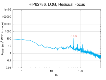
Figure 7: PSDs of closed-loop AO measurements for focus (blue), with estimated error amount (red annotation) at 60 Hz. With cryocoolers on at full power (top left) and an integral controller, the 60 Hz focus error was 90 nm rms. With cryocoolers at low power (top right), the error is reduced to 51 nm rms. Use of the LQG controller with cryocoolers at full power reduces the 60 Hz term to 3 nm rms, which is now a negligible amount. Telemetry: _When_2014.5.13_0.3.53, _When_2014.5.13_0.25.28 and _When_2014.5.13_0.10.18.

Annotated in red is the estimate error that is sent on to the science leg from the 60 Hz component. At upper left is on-sky operation with an integral controller for the FOcus control. In this case the 60 Hz error leads to a time-average of 90 nm rms wavefront error due to focus. When the cryocoolers are turned down, but not off, the amount of focus at 60 Hz is reduced to 51 nm. (When the cryocoolers are turned off completely this amount is 0 nm; due to system constraints we were not able to test this option as well on this target.) With the cryocoolers at normal and the LQG, the deep notch (see Figure 1, left panel) strongly rejects the 60 Hz signal. In this case the result (bottom panel of figure) is just 3 nm. This level is negligible in terms of the overall error budget.

Two more items remain in the validation of the focus control. First, we still do not have definitive science images that show the difference between LQG on and off. Second, the exact spatial shape of the error to be corrected, that is not just focus but some combination of focus, trefoil and sphere, could be refined.

8 Error budget

We have developed a provisional error budget. These numbers are generated from analysis of closed-loop AO measurements following the methods outlined in Section 2 to convert from measurements to estimated error passed on to the science leg.

Table 2: Error budget. Important observational parameters given in top panel. Error amounts in nm rms wavefront as determined from AO telemetry in second panel. Telemetry used: a: _When_2014.3.22_21.58.10; b: _When_2013.12.11_3.30.29; c: _When_2014.3.22_7.18.5; d: _When_2014.3.24_2.37.15; e: _When_2014.5.14_20.1.4.

Target	$\beta$ Pictorisa	$\beta$ Pictorisb	HD141569c	HIP59563d	HD101615e
Star I-band mag	3.9	3.9	7	9	5.6
Gains	OFC	OFC	0.2	OFC	OFC
Frame rate	1 kHz	1 kHz	1 kHz	500 Hz	1 kHz
cryocoolers	On	Low	Off	On	On
LQG	Off	Off	Off	Off	On
Seeing	best	normal	normal	normal	normal
Servo-lag error	25	48	61	99	55
AOWFS noise	6	7	24	52	16
Static error	12	11	16	16	9
60 Hz vibrations	109	51	0	88	31

Error estimates are given in Table 2 for five different observations. For each observation the star name and magnitude is given. Modal gain optimization (“OFC”) was used in four of the five cases, though on targets brighter than 7th this essentially is the same as uniform gains of value 0.3.

The first observation of $\beta$ Pictoris from March represents performance in very good seeing - we were able to use the spatial filter at 2.8 mm stably for several minutes, and servo lag error was estimated to be just 25 nm. During more typical seeing on a bright to moderate target with loop gains at maximum, the servo lag error is around 50 nm (second $\beta$ Pictoris, HD101615, HD141569).

The HIP59563 observation (the same one used in Section 4 for testing the gain optimizer) is representative of our performance on the dimmest target required of GPI. At 500 Hz with optimized gains we have 99 nm of servo lag error and 52 nm of WFS noise. With cryocoolers at normal power with no LQG, science leg error from the 60 Hz phase is generally between 80 and 120 nm (depends on conditions and orientation). With cryocoolers off this is reduced to 0; with the LQG as tested in May on the focus shape, there are 31 nm of 60 Hz phase leftover - this is dominated by trefoil and spherical. As noted above, this may be reduced further, but it is no longer a dominant term in the AO error budget.

The telemetry for HD141569 was taken co-incident with an non-coronagraphic image, which is shown in Figure 8.

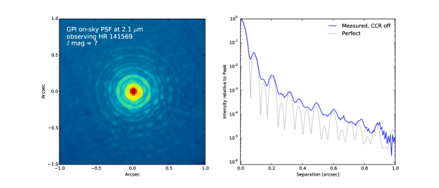
Figure 8: GPI narrow-band point spread function at 2.1 microns for a 7th magnitude star, as observed with the GPI IFS [39] and reduced with the GPI Data Reduction Pipeline [40]. Total exposure time was 45 s, obtained as 1.5 s * 10 coadds plus 5 s * 6 coadds for increased dynamic range. This is a synthetic narrow band image obtained by integrating over a small range of wavelengths in the data cube ($\lambda_{c}=2.10\mu$m, $\lambda/\Delta\lambda=30$). In an azimuthally-averaged radial profile up to 15 Airy rings can be detected, as shown at right. The grey curve shows the theoretical perfect PSF for the Gemini South telescope aperture geometry, integrated over the same spectral bandpass.

The Strehl of this image has not been rigorously estimated at this time. However, up to 15 Airy rings can be detected in the narrow-band image, indicating that the AO system is performing well. We estimate the fitting [41] and aliasing error[24] terms from theory using the coefficient of 0.3, such that $\sigma^{2}_{\mathrm{fitting}}=0.3(d/r_{0})^{5/3}$ and $\sigma^{2}_{\mathrm{aliasing}}=0.33\sigma^{2}_{\mathrm{fitting}}$. We assume that $r_{0}$ was 14 cm for the typical seeing conditions. For the HD141569 observation this gives us a fitting error of 54 nm and an aliasing error of 31 nm. Adding in the assumed 30 nm non-common-path errors given in Macintosh [1], we add in quadrature to the terms in the HD141569 column of the table: $(54^{2}+31^{2}+61^{2}+24^{2}+16^{2}+0^{2}+30^{2})^{1/2}=97$ nm. At 2.1 microns, this is a Strehl of 92%.

We reiterate that we do not have a direct measurement of fitting error, aliasing error of non-common-path errors, but are using our best estimate at this time. In future work we plan to improve it through better estimates of seeing (and hence fitting), better examination of the aliasing error through analysis of telemetry, and improved information on the non-common-path error. These improved estimates will be accompanied by analysis of the co-incident science images, which was beyond the scope of this work.

9 Conclusions

GPI’s AO system features several new technologies. During its verification and commissioning period we have systematically tested these technologies and analyzed performance. The computationally efficient FTR method of wavefront reconstruction is successful, though we have to remove rotation from the centroids to prevent driving a scalloped shape on the Tweeter when the spot size changes (due to either bias level or spot size due to seeing). The modal gain optimization method updates 2304 modal gains for the Fourier modes every 8 seconds in closed loop. Tests have shown that the optimizer is correctly finding gains for each individual mode that minimize the error, and also minimizing overall error. Modal gain filters show clear evidence of wind.

The AO system uses an LQG controller for tip, tilt and focus to reject vibrations. For tip and tilt we correct common-path vibrations at 60, 120 and 180 Hz to under 1 mas per axis. By pulling focus out of the centroids and sending it through the LQG, we can very strongly reject the focus at 60 Hz , reducing it to just 3 nm rms wavefront error. There is some 60 Hz phase left over (trefoil and spherical) that could be further reduced if it helps overall performance. The spatially-filtered wavefront sensor has under-performed relative to our expectations. We have clear evidence, thanks to layers of frozen flow turbulence, that the spatial filter does reject aliases. However, we are not able to regularly use the spatial filter stably at it nominal $\lambda/d$ diameter. In very good seeing we can get it down to 2.8 mm, but it is more typical that we use it at 3.5 mm. At this size it clears out aliasing from the inner 42% of the dark hole (i.e. to radius $0.42\lambda/d$ instead of $\lambda/d$.) We have presented an provisional error budget of AO terms that we can directly measure. On bright to moderate targets (down to around 7th magnitude), performance is dominated by servo lag error. In typical seeing this term is 50 nm. On dimmer targets the gain optimizer will trade off servo lag and WFS noise. On our dimmest required target of 9th magnitude we achieved 99 nm servo lag error and 52 nm WFS noise.

We will continue to work during the end of the verification and commissioning period to analyze existing science images and obtain new ones as necessary to confirm our analysis, which is here based on AO telemetry. Of particular interest are verifying the impact of the focus LQG, which on most targets removes the dominant 60 Hz term in the error budget. We also want to quantify contrast in longer exposures as a function of spatial filter size and determine if we can do better than 3.5 mm, which is oversized by about 60%.

- [1] Macintosh, B. and Graham, J. R. and Ingraham, P. and Konopacky, Q. and Marois, C. and Perrin, M. and Poyneer, L. and Bauman, B. and Barman, T. and Burrows, A. and Cardwell, A. and Chilcote, J. and De Rosa, R. J. and Dillon, D. and Doyon, R. and Dunn, J. and Erikson, D. and Fitzgerald, M. and Gavel, D. and Goodsell, S. and Hartung, M. and Hibon, P. and Kalas, P. G. and Larkin, J. and Maire, J. and Marchis, F. and Marley, M. and McBride, J. and Millar-Blanchaer, M. and Morzinski, K. and Norton, A. and Oppenheimer, B. R. and Palmer, D. and Patience, J. and Pueyo, L. and Rantakyro, F. and Sadakuni, N. and Saddlemyer, L. and Savransky, D. and Serio, A. and Soummer, R. and Sivaramakrishnan, A. and Song, I. and Thomas, S. and Wallace, J. K. and Wiktorowicz, S. and Wolff, S., “First light of the Gemini Planet Imager,” Proceedings of the National Academy of Sciences (2014).
- [2] Beuzit, J.-L., Feldt, M., Dohlen, K., Mouillet, D., Puget, P., Wildi, F., Abe, L., Antichi, J., Baruffolo, A., Baudoz, P., Boccaletti, A., Carbillet, M., Charton, J., Claudi, R., Downing, M., Fabron, C., Feautrier, P., Fedrigo, E., Fusco, T., Gach, J.-L., Gratton, R., Henning, T., Hubin, N., Joos, F., Kasper, M., Langlois, M., Lenzen, R., Moutou, C., Pavlov, A., Petit, C., Pragt, J., Rabou, P., Rigal, F., Roelfsema, R., Rousset, G., Saisse, M., Schmid, H.-M., Stadler, E., Thalmann, C., Turatto, M., Udry, S., Vakili, F., and Waters, R., “SPHERE: a ’planet finder’ instrument for the VLT,” (2008).
- [3] Oppenheim, A. V., Schafer, R. W., and Buck, J. R., [Discrete-time Signal Processing ], Prentice Hall, New Jersey (1999).
- [4] Poyneer, L. A. and Véran, J.-P., “Optimal modal Fourier transform wave-front control,” J. Opt. Soc. Am. A 22, 1515–1526 (2005).
- [5] Freischlad, K. and Koliopoulos, C. L., “Wavefront reconstruction from noisy slope or difference data using the discrete fourier transform,” Proc. SPIE 551, 74–80 (1985).
- [6] Freischlad, K. and Koliopoulos, C. L., “Modal estimation of a wave front from difference measurements using the discrete fourier transform,” J. Opt. Soc. Am. A 3, 1852–1861 (1986).
- [7] Poyneer, L. A., Gavel, D. T., and Brase, J. M., “Fast wave-front reconstruction in large adaptive optics systems with use of the Fourier transform,” J. Opt. Soc. Am. A 19, 2100–2111 (2002).
- [8] Poyneer, L. A., “Advanced techniques for Fourier transform wave-front reconstruction,” Proc. SPIE 4839, 1023–1033 (2002).
- [9] Poyneer, L. A., Signal processing for high-precision wavefront control in Adaptive Optics, PhD thesis, University of California, Davis (June 2007).
- [10] Ellerbroek, B. L., “Efficient computation of minimum-variance wave-front reconstructors with sparse matrix techniques,” J. Opt. Soc. Am. A 19, 1803–1816 (2002).
- [11] Lavinge, J.-F. and Véran, J.-P., “Woofer-tweeter control in an adaptive optics system using a Fourier reconstructor,” J. Opt. Soc. Am. A 25(9), 2271–2279 (2008).
- [12] Poyneer, L. A., Véran, J.-P., Dillon, D., Severson, S., and Macintosh, B. A., “Wavefront control for the Gemini Planet Imager,” Proc. SPIE 6272, 62721N (2006).
- [13] Savransky, D., Thomas, S. J., Poyneer, L. A., and Macintosh, B. A., “Computer vision applications for coronagraphic optical alignment and image processing,” Appl. Opt. 52, 3394–3403 (May 2013).
- [14] Sadakuni, N., Macintosh, B. A., Palmer, D. W., Poyneer, L. A., Max, C. E., Savransky, D., Thomas, S. J., Cardwell, A., Goodsell, S., Hartung, M., Hibon, P., Rantakyrö, F., and Serio, A., “Effects of differential wavefront sensor bias drifts on high contrast imaging,” Proc. SPIE 9148 (2014).
- [15] Greenbaum, A. Z., Cheetham, A., Sivaramakrishnan, A., Tuthill, P., Norris, B., Pueyo, L., Rantakyrö, F., Hibon, P., Goodsell, S., Hartung, M., Serio, A., Cardwell, A., Poyneer, L., Macintosh, B., Sravansky, D., Perrin, M., Wolff, S., Ingraham, P., and Thomas, S., “Gemini Planet Imager observational calibrations X: Commissioning & performance analysis of GPI NRM,” Proc. SPIE 9147 (2014).
- [16] Gendron, E. and Léna, P., “Astronomical adaptive optics I. Modal control optimization,” Astron. Astrophys. 291, 337–347 (1994).
- [17] Gendron, E. and Léna, P., “Astronomical adaptive optics II. Experimental results of an optimized modal control,” Astron. Astrophys. Suppl. Ser. 111, 153–167 (1995).
- [18] Véran, J.-P., “Altair’s optimiser,” tech. rep., Herzberg Institute of Astrophysics, Victoria, BC, Canada (1998).
- [19] Rousset, G., Lacombe, F., Puget, P., Hubin, N. N., Gendron, E., Fusco, T., Arsenault, R., Charton, J., Feautrier, P., Gigan, P., Kern, P. Y., Lagrange, A., Madec, P., Mouillet, D., Rabaud, D., Rabou, P., Stadler, E., and Zins, G., “NAOS, the first AO system of the VLT: on-sky performance,” Proc. SPIE 4839, 140–149 (2003).
- [20] Esposito, S., Riccardi, A., Pinna, E., Puglisi, A. T., Quirós-Pacheco, F., Arcidiacono, C., Xompero, M., Briguglio, R., Busoni, L., Fini, L., Argomedo, J., Gherardi, A., Agapito, G., Brusa, G., Miller, D. L., Guerra Ramon, J. C., Boutsia, K., and Stefanini, P., “Natural guide star adaptive optics systems at lbt: Flao commissioning and science operations status,” (2012).
- [21] Poyneer, L. A. and Macintosh, B. A., “Optimal Fourier Control performance and speckle behavior in high-contrast imaging with adaptive optics,” Opt. Exp. 14, 7499–7514 (2006).
- [22] Poyneer, L. A., Bauman, B., Cornelissen, S., Isaacs, J., Jones, S., Macintosh, B. A., and Palmer, D. W., “The use of a high-order MEMS deformable mirror in the Gemini Planet Imager,” Proc. SPIE 7931, 793104 (2011).
- [23] Morzinski, K. M., Evans, J. W., Severson, S., Macintosh, B., Dillon, D., Gavel, D., Max, C., and Palmer, D., “Characterizing the potential of MEMS deformable mirrors for astronomical adaptive optics,” Proc. SPIE 6272, 627221 (2006).
- [24] Rigaut, F. J., Véran, J.-P., and Lai, O., “Analytical model for Shack-Hartmann-based adaptive optics systems,” Proc. SPIE 3353, 1038–1048 (1998).
- [25] Jolissaint, L., Véran, J.-P., and Conan, R., “Analytical modeling of adaptive optics: foundations of the phase spatial power spectrum approach,” J. Opt. Soc. Am. A 23(2), 382–394 (2006).
- [26] Poyneer, L. A. and Macintosh, B., “Spatially filtered wave-front sensor for high-order adaptive optics,” J. Opt. Soc. Am. A 21, 810–819 (2004).
- [27] Fusco, T., Petit, C., Rousset, G., Conan, J.-M., and Beuzit, J.-L., “Closed-loop experimental validation of the spatially filtered Shack-Hartmann concept,” Opt. Lett. 30, 1255–1257 (2005).
- [28] Poyneer, L. A., Bauman, B., Macintosh, B. A., Dillon, D., and Severson, S., “Experimental demonstration of phase correction with a 32 x 32 microelectricalmechanical systems mirror and a spatially filtered wavefront sensor,” Opt. Lett. 31, 293–295 (2006).
- [29] Poyneer, L. A., van Dam, M. A., and Véran, J.-P., “Experimental verification of the frozen flow atmospheric turbulence assumption with use of astronomical adaptive optics telemetry,” J. Opt. Soc. Am. A 26, 833–846 (2009).
- [30] Gavel, D. T. and Wiberg, D., “Towards strehl-optimizing adaptive optics controllers,” Proc. SPIE 4839, 890–901 (2002).
- [31] Le Roux, B., Conan, J.-M., Kulcsár, C., Raynaud, H.-F., Mugnier, L. M., and Fusco, T., “Optimal control law for classical and multiconjugate adaptive optics,” J. Opt. Soc. Am. A 21, 1261–1276 (2004).
- [32] Petit, C., Conan, J. M., Kulcsár, C., Raynaud, H. F., and Fusco, T., “First laboratory validation of vibration filtering with LQG control law for adaptive optics,” Opt. Exp. 16, 87–97 (2008).
- [33] Sivo, G., Kulcsár, C., Conan, J.-M., Raynaud, H.-F., Gendron, E., Basden, A., Vidal, F., Morris, T., Meimon, S., Petit, C., Gratadour, D., Martin, O., Hubert, Z., Rousset, G., Dipper, N., Talbot, G., Younger, E., and Myers, R., “Full lqg control with vibration mitigation: From theory to first on-sky validation on the canary moao demonstrator,” in [Imaging and Applied Optics ], Imaging and Applied Optics , OTu2A.2, Optical Society of America (2013).
- [34] Guesalaga, A., Neichel, B., O’Neal, J., and Guzman, D., “Mitigation of vibrations in adaptive optics by minimization of closed-loop residuals,” Opt. Express 21, 10676–10696 (May 2013).
- [35] Poyneer, L. A. and Véran, J.-P., “Predictive wavefront control for adaptive optics with arbitrary control loop delays,” J. Opt. Soc. Am. A 25, 1486–1496 (2008).
- [36] Poyneer, L. A. and Véran, J.-P., “Kalman filtering to suppress spurious signals in adaptive optics control,” J. Opt. Soc. Am. A 27(11), A223–A234 (2010).
- [37] Correia, C., Raynaud, H.-F., Kulcsár, C., and Conan, J.-M., “Minimum-variance control for woofer–tweeter systems in adaptive optics,” J. Opt. Soc. Am. A 27(11), A133–A144 (2010).
- [38] Hartung, M., Saddlemyer, L., Hayward, T., Macintosh, B. A., Poyneer, L. A., Guesalaga, A., Savransky, D., Sadakuni, N., Dillon, D., Wallace, J. K., Galvez, R., Gausachs, G., Collins, O., Cardwell, A., Serio, A., Rantakyrö, F. T., and Goodsell, S., “On-sky vibration environment for the Gemini Planet Imager and mitigation effort,” Proc. SPIE 9148 (2014).
- [39] Larkin, J. E., Chilcote, J. K., Aliado, T., Bauman, B. J., Brims, G., Canfield, J. M., Dillon, D., Doyon, R., Dunn, J., Fitzgerald, M. P., Graham, J. R., Goodsell, S., Hartung, M., Ingraham, P., Johnson, C. A., Kress, E., Konopacky, Q. M., Macintosh, B. A., Magnone, K. G., Maire, J., McLean, I. S., Palmer, D., Perrin, M. D., Quiroz, C., Sadakuni, N., Saddlemyer, L., Thibault, S., Thomas, S. J., Vallee, P., and Weiss, J. L., “The Integral Field Spectrograph for the Gemini Planet Imager,” Proc. SPIE 9147 (2014).
- [40] Perrin, M., Maire, J., Ingraham, P. J., Savransky, D., Millar-Blanchaer, M., Wolff, S. G., Ruffio, J.-B., Wang, J. J., Draper, Z. H., Sadakuni, N., Marois, C., Rajan, A., Fitzgerald, M. P., Macintosh, B., Graham, J. R., Doyon, R., Larkin, J. E., Chilcote, J. K., Goodsell, S. J., Palmer, D. W., Labrie, K., Beaulieau, M., Rosa, R. J. D., Greenbaum, A. Z., Hartung, M., Hibon, P., Konopacky, Q. M., Lafreniere, D., Lavigne, J.-F., Marchis, F., Patience, J., Pueyo, L. A., Rantakyro, F., Soummer, R., Sivaramakrishnan, A., Thomas, S. J., Ward-Duong, K., and Wiktorowicz, S., “Gemini Planet Imager observational calibrations I: overview of the GPI data reduction pipeline,” Proc. SPIE 9147 (2014).
- [41] Hardy, J. W., [Adaptive Optics for Astronomical Telescopes ], Oxford University Press, New York (1999).