Gemini Planet Imager Observational Calibrations VI: Photometric and Spectroscopic Calibration for the Integral Field Spectrograph

Résumé

The Gemini Planet Imager (GPI) is a new facility instrument for the Gemini Observatory designed to provide direct detection and characterization of planets and debris disks around stars in the solar neighborhood. In addition to its extreme adaptive optics and coronagraphic systems which give access to high angular resolution and high-contrast imaging capabilities, GPI contains an integral field spectrograph providing low resolution spectroscopy across five bands between 0.95 and 2.5 $\mu$m. This paper describes the sequence of processing steps required for the spectro-photometric calibration of GPI science data, and the necessary calibration files. Based on calibration observations of the white dwarf HD 8049 B we estimate that the systematic error in spectra extracted from GPI observations is less than 5%. The flux ratio of the occulted star and fiducial satellite spots within coronagraphic GPI observations, required to estimate the magnitude difference between a target and any resolved companions, was measured in the $H$-band to be $\Delta m=9.23\pm 0.06$ in laboratory measurements and $\Delta m=9.39\pm 0.11$ using on-sky observations. Laboratory measurements for the $Y$, $J$, $K1$ and $K2$ filters are also presented. The total throughput of GPI, Gemini South and the atmosphere of the Earth was also measured in each photometric passband, with a typical throughput in $H$-band of 18% in the non-coronagraphic mode, with some variation observed over the six-month period for which observations were available. We also report ongoing development and improvement of the data cube extraction algorithm.

1 Introduction

The combination of high angular resolution and high-contrast imaging, made possible by tremendous improvements in the performance of adaptive optics (AO) systems [1, 2, 3] and developments of coronagraphic capabilities[4, 5, 6], is opening a new window into studying the formation and evolution processes of planetary systems by exploring and characterizing the exoplanet population at large orbital separation (beyond several AU). Direct imaging observations are particularly valuable because they enable spectroscopic characterization of the detected planetary-mass companions[7, 8, 9]. Several exoplanets have been already directly imaged [10, 11, 12, 13, 14], but the required extreme contrast ratio required at very small angular separations remains a major obstacle in the detection of new companions.

The Gemini Planet Imager[15, 16, 17, 18] (GPI) is a new high angular resolution extreme adaptive optics instrument that provides unprecedented high-contrast capabilities. After a successful installation at Gemini South in October 2013, the GPI team performed four commissioning observing runs to assess the performance of the instrument, followed by an early science observing run open to the community. GPI’s science instrument is an integral field spectrograph (IFS) that can observe in one of the near-infrared $Y$, $J$, $H$, $K1$, $K2$ filter bandpasses. In its spectral mode, the IFS makes use of a lenslet array and a prism [19, 20] to subdivide its 2.7”$\times$2.7” field of view into 192$\times$192 spectra, with a plate scale of 14.3 mas/pixel [21], and a spectral resolving power ranging from $\lambda/d\lambda=35$ to 90[22], depending on the band. Because of the increased resolution at longer wavelengths the $K$ band is split into two partially overlapping bandpasses for GPI; $K1$ ($1.9-2.2$ $\mu$m) and $K2$ ($2.1-2.4$ $\mu$m). The micro-lens array is rotated by 24.8 degrees with respect to the detector to maximize the number of spectra on the detector, and to optimize the distance between them. In polarimetric mode, the spectral prism is replaced by a Wollaston prism and a rotating half-wave plate is inserted into the beam in order to measure the polarization of the incoming light[23].

The reduction of GPI IFS raw science images, containing $\sim$37,000 spectra, is a complex process that involves the need for accurate calibrations. The GPI Data Reduction Pipeline[24, 25] (DRP) has been developed to produce calibrated datacubes with minimal processing artifacts, ready for scientific analysis. This paper describes the steps necessary to perform photometric (Section 2) and spectroscopic (Section 3) calibration of reduced GPI IFS data. The absolute calibration of the fiducial satellite spots, necessary for measuring companion magnitudes and contrast, is discussed in Section 4. The throughput of the instrument is measured in Section 5, and a new method of spectral extraction implemented in the pipeline utilizing micro-lens PSFs to reduce systematics is presented in Section 6.

2 GPI Photometric calibration

Several steps are necessary to transform the raw two-dimensional GPI IFS detector images containing the micro-spectra into three-dimensional spectrophotometrically calibrated datacubes. The first steps are for mitigating detector noise that affects the raw images to remove correlated noise and detector artifacts. A detailed characterisation of this source of noise and methods to reduce its effect are fully described in Ingraham et al. 2014[26]. These corrections are more naturally performed directly on the IFS raw two-dimensional images, since this noise is directly engendered by, or related to the detector.

HAWAII-2RG detectors generate dark current, smaller than 0.1 e^-/s/pixel, that produces a mean fixed pattern in the image during an exposure. Master dark frames are produced daily, at exposure times ranging from 1.45 s to 120 s, which are used to correct observations with the “Subtract dark background” primitive within the GPI DRP. Other sources of noise, such as high-frequency striping due to readout electron noise and microphonic vibrations induced by the cryo-coolers[22] are removed using the “Destripe science image” primitive on images that contain enough non-illuminated pixels to derive a noise model. Defective pixels are identified using the periodically updated GPI bad pixel map, and their intensities are corrected by the primitive “Interpolate bad pixels in 2D frame” using surrounding pixel intensities to interpolate the intensity of the defective pixel. Other effects, such as persistence can also be corrected[26], whereas effects such as non-linearity are best avoided by maintaining the total number of counts per pixel below $\sim$17,000 ADU/coadd, or by allowing the persistence to diminish after a sequence of saturated exposures.

The datacube extraction procedure requires the location of the $\sim$37,000 spectra within the raw image, for each filter used, to an accuracy of better than a tenth of a pixel[27]. The separation between the individual spectra on the raw image is $4.5$ pixels at the center of the image. Field-dependent aberrations induced by the re-imaging optics after the lenslet array result in the tilt of the micro-spectra changing as a function of their position on the detector. This results in the inter-spectra separation varying slightly over the field. Measured wavelength solutions for each band are provided from the reduction of Gemini GCAL xenon and argon lamps. The locations of the spectra given by the wavelength solution are corrected for instrumental flexure effects that shift the spectra on the detector as the orientation of the instrument varies[27]. Light passing through each micro-lens is diffracted and the resulting point spread function (PSF) spreads over several detector pixels, with a typical 1.5 pixel full width at half maximum (FWHM) in $H$-band ($1.5-1.8$ $\mu$m). The original method of datacube extraction implemented into the GPI pipeline proceeds by integrating the signal over a rectangular 1$\times$3 pixel aperture centered on the spectrum, a process which is repeated for each pixel along the dispersion axis to produce the final spectrum. The length of the photometric rectangular aperture was therefore chosen to integrate the maximal number of pixels covering the extent of the micro-lens PSF at the wavelength of interest, and small enough to limit the contamination from the PSF wings coming from surrounding spectra. Once the spectra have been separately extracted, they are interpolated onto a common wavelength axis and assembled into a datacube. The steps discussed above are accomplished using a combination of primitives “Load Wavelength Solution”, “Update Spot Shifts for Flexure”, “Assemble Spectral Datacube” and “Interpolate Wavelength Axis”, and allows for the pipeline to produce a reduced datacube in few seconds using a standard desktop or laptop computer. Since no matrix inversion is required, the method is extremely robust, avoiding any noise amplification or convergence issues that can happen with standard inversion methods. However, this method is partially affected by the small spacing between spectra, especially at the corners of the field-of-view, where the spectra are highly tilted with respect to the spectral axis and contamination from surrounding spectra becomes more significant. Based on simulations of raw IFS images where the light coming from one micro-lens was artificially blocked, we measured the contamination from adjacent micro-lenses to be less than 2%.

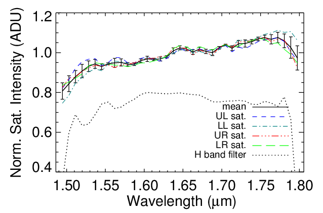
Figure 1: The individual extracted spectra for the four satellite spots, normalized to have equal integrated intensity over the band. The uncertainties from satellite spectra are propagated into the extracted spectra of companions. The UL, UR, LL, LR acronyms indicate the upper left, upper right, lower left, and lower right satellite, respectively. The dotted curve represents the H-band filter profile with the peak transmission normalized to 0.8 for ease of comparison to the satellite spot spectra.

As the micro-lens PSF extends over several pixels along the spectral axis as well, internal cross-talk between spectral channels of the same micro-spectrum occurs when using the integration method, especially for spectra with strong features. This cross-talk impacts adjacent spectral channels and affects the spectral resolution. The length of the spectra, about $\sim$18 pixels in the $H$-band, results in a detector-pixel-limited Nyquist sampled spectral resolution about $\sim$$50\pm 6$ in $H$-band, depending the location in the field-of-view. The datacube generated by the GPI DRP contains 37 spectral channels which are spectrally oversampled by a factor $\sim$2 relative to the detector sampling. It is possible to reach slightly better resolving power by taking into account of the micro-lens PSF extent in the datacube extraction process (see Section 6).

It should be noted that the flat-field correction methods for GPI data are still in development. Multiple factors contribute different types of flat fields, including in particular the lenslet array flat and the detector pixel flat. Because of shifts of the spectra due to flexure effects, the detector pixels illuminated when observing a daytime calibration flat-field are not necessarily the same ones illuminated in any particular science image of interest. This results in different pixel sensitivities in the flat-field and science frames. Consequently, it is recommended to only use a master flat-field that has exactly the same locations of spectra in the raw frames than those for the science image to be corrected. This could be obtained by taking images using the flat-field lamp just before and/or after the target observations at similar elevations, under the assumption that the flexure effect will remain stable during the course of those observations.

Separately, a lenslet flat field can be derived to account for the varying illumination through the lenslet array. A handful of scattered lenslets have lower than average throughput which can be compensated for. Furthermore, an artifact from the manufacturing process for the lenslet array is that every 30th row and 50th column has slightly higher throughput than average, each accompanied by a slightly fainter adjacent row or column. We interpret these as the boundaries between replicated blocks of 30$\times$50 lenslets. The observed effect is small, with a throughput variations for the affected rows and columns of $\sim 0.5\%$. This can be compensated for using the lenslet flat field, though it is a small enough correction to be negligible in many circumstances.

In coronagraphic mode, the absolute photometric calibration takes advantage of the presence of fiducial satellite spots, produced by the diffraction of light from a square grid printed onto the apodizer[28, 29]. These four satellite spots represent four images of the unocculted host star, scaled in intensity by a known factor, or grid ratio, measured in the lab. Together with the spectral type and apparent magnitude, they permit an astrometric and photometric calibration of the data. The laboratory and on-sky measurement of the grid ratio is given in Section 4, with a detailed discussion on the stability of the photometry of these fiducial spots given in Wang et al. 2014 (this proceedings[30]). Once the fiducial spot mean intensity has been measured in each slice of the datacube, it is possible to use the grid ratio to estimate the number of counts that an image of the unocculted star would have produced.

The DRP primitive “Calibrate Photometric Flux” uses the grid ratio, photometry of the spots at each wavelength, gain of the detector, exposure time, collecting area of the telescope, and the magnitude and spectral type of the occulted star to perform the photometric calibration, compensating for the instrumental and atmospheric transmission functions and converting measured ADU into a variety of commonly-used physical units (photons/s/nm/m², Jy, W/m²/$\mu$m, ergs/s/cm²/$\mathrm{\SIUnitSymbolAngstrom}$ and ergs/s/cm²/Hz). The pipeline contains a copy of the Pickles stellar spectral flux library [31] for a wide range of stellar spectral types to be used as part of the calibration, but also permits the use of user-defined spectra. Surface brightness units may be obtained simply by normalizing by the area of each lenslet, 14.3 mas².

3 GPI Spectroscopic Calibration

Determining the accuracy of the spectroscopic extraction of GPI spectra is required to assign uncertainties to our spectral data. The primary challenge in characterizing the spectral extraction performance is to understand the systematic errors that may result from each step in the reduction process. Observations of standard stars are used to test the quality of spectral extraction, but GPI is observing in a parameter space that is beyond the separation and contrast limits of previous imagers. Therefore only a small number of previously observed standards exist; several of which are cooler L and T-type brown dwarfs that do not have well-understood spectra. Of the known close companions, the few white dwarfs are most attractive for spectral characterization given their well-understood atmospheres.

As part of the GPI Verification and Commissioning stage, the white dwarf companion to HD 8049 was observed to asses the accuracy of spectroscopic retrieval from GPI IFS data reduced using the DRP. Previous observations[32] have constrained the white dwarf (HD 8049 B) to have an effective temperature of $18,800\pm 2,100$ K, and the spectrum is consistent with a blackbody of the same temperature. This target represents an ideal calibration source for GPI. The dataset consists of five 90s $H$-band exposures of HD 8049 taken on December 10, 2013. For this data, zero-point offsets to the wavelength solutions were determined using an argon arclamp image taken immediately following the exposures. The dark subtracted detector images had their micro-spectra extracted using the 3-pixel box extraction algorithm. The individual cubes were then stacked in two different ways. The first method was a straight median stack resulting in a higher signal to noise of the satellites and speckles, but a spectral smearing of the companion. The second stack was created by first rotating each image such that North was in the vertical direction prior to performing the median. This ensured a higher signal-to-noise ratio (SNR) of the companion, while blurring the speckles and satellites. These two cubes were then input into the DRP primitive “Calibrate Photometric Flux” that both detects the satellites and extracts their spectra, then in combination with a designated spectral type and apparent magnitude of the primary star, outputs a spectrophotometrically calibrated version of the derotated median cube. Figure 1 shows the four extracted spectra of the satellite spots normalized to have the same integrated intensity, with the mean value plotted as the solid black line and the error bars signifying the standard deviation between the four points. In the case of Figure 1, the spectra have been normalized for ease of comparison over the full wavelength range. The error bars shown here do not include the error component of each individual satellite which is derived from looking at the standard deviation of an arc shaped region surrounding the satellite, convolved by the extraction aperture.

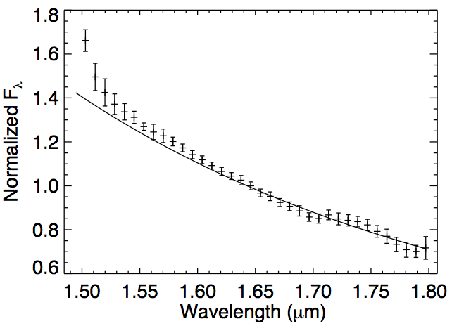
Figure 2: The calibrated $H$-band spectrum of HD 8049 B overplotted with a 18,800 K blackbody (solid line).

The GPI pipeline extracts the spectral data over the range in wavelengths that has a filter transmission of 10% or higher. This results in a significant decrease in the SNR towards the edge of the bands, where the filter transmission drops sharply. Large systematic errors may result when calibrating the cube towards the filter edges in the regions of dropping transmission, particularly if there are small errors in the wavelength calibration. For these reasons, we advise users to exercise caution and trim their data according to the quality and SNR of their spectra and wavelength calibration. We have opted to leave the wavelengths with 10% transmission as part of the cubes intentionally so that users may exercise their own judgement on the usable wavelength region, rather than imposing sharp cutoff by the pipeline at some higher throughput.

Obtaining an absolute flux calibration requires knowledge of the satellite spot to star flux ratio, a value which has shown variability in the past in shape and is the subject of investigation as part of GPI commissioning. Further details regarding the satellite spots are given in Section 4 and in Wang et al. 2014 (this proceedings[30]). The pipeline is currently using satellite spot to star flux ratios that were measured during the integration and testing of the instrument, although on-sky measurements obtained during commissioning show similar values (shown in Table 1 and discussed in section 4). The pipeline values will be updated to reflect new on-sky measurements in an upcoming pipeline release.

Extracting a spectrum from a calibrated datacube is performed using the DRP primitive, “Extract 1d spectrum.” This primitive uses the same extraction aperture (by default) as is in extracting the satellite spot spectra to ensure no introduction of systematic errors from aperture corrections. The uncertainty computed by the primitive combines the uncertainty from the satellite spot spectra along with an uncertainty of the noise surrounding the companion. Figure 2 shows the calibrated $H$-band spectrum of HD 8049 B overplotted with an 18,800 K blackbody. Overall, the fit is of high quality, but exhibits a reduced $\chi^{2}$ of 2.00 due to the data points on the blue end of the spectrum that are in a region of low throughput and obvious victim of the systematic error discussed above. If we restrict the wavelength range of the data to the region where transmission function is smooth and above 50% ($1.51\leavevmode\nobreak\ \mu\text{m}<\lambda<1.79\leavevmode\nobreak\ \mu\text{m}$), the resulting reduced $\chi^{2}$ is 1.07, demonstrating that the model is well represented by the data. Another systematic present in the data is a small increase in flux near 1.73 $\mu$m. This is believed to be a systematic bias due to datacube extraction, but analysis into this is ongoing. Current estimates of the systematic errors contained in the pipeline, arising primarily from the extraction algorithm, are estimated to be $<5\%$ based on this dataset. More advanced extraction algorithms, such as what is described in section 6 and by Draper et al. 2014 (this proceedings [34]) are in development and are expected to significantly decrease the systematic errors.

4 GPI Fiducial Spot Calibration

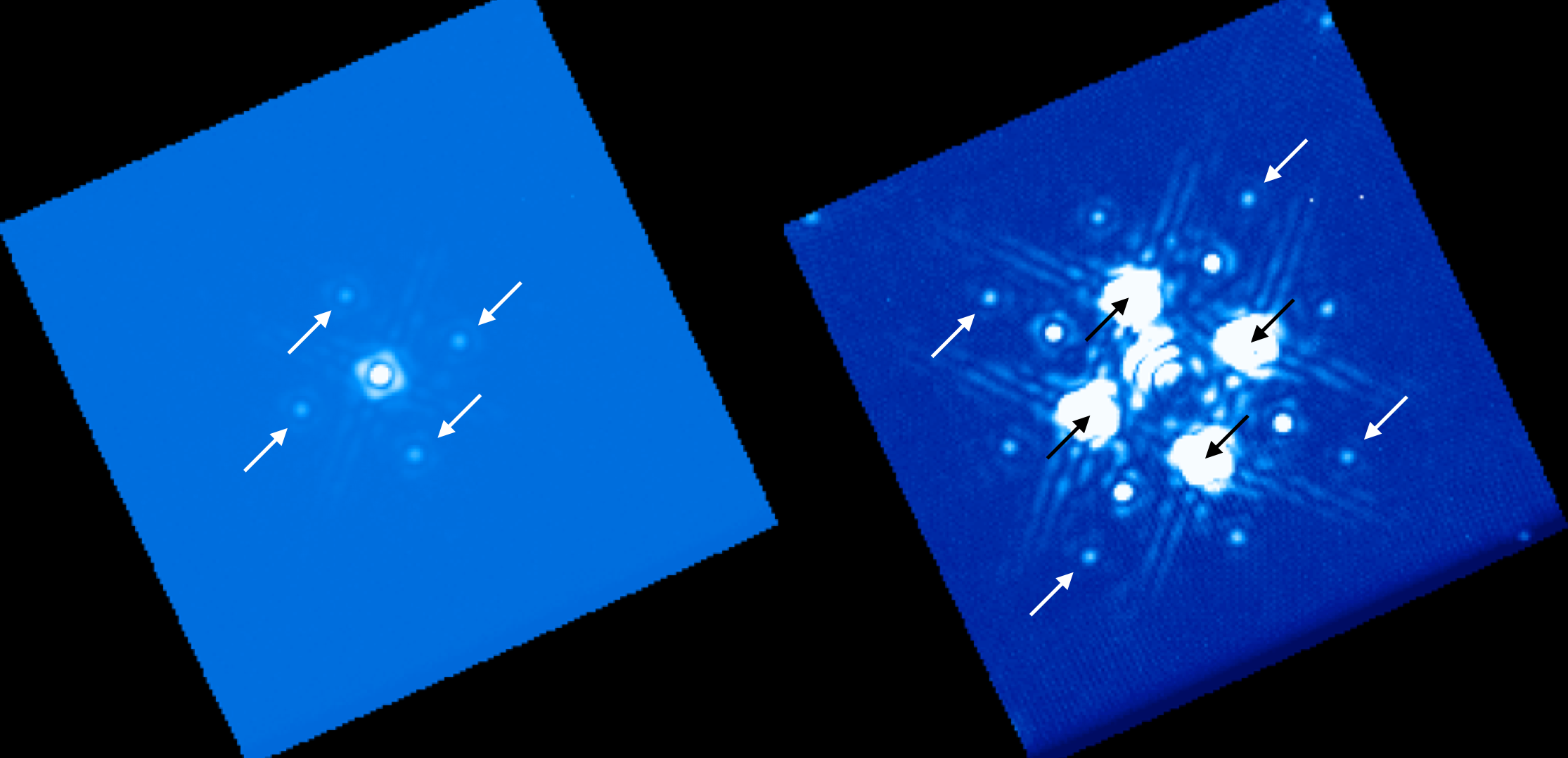
Figure 3: (left panel) Laboratory measurement of the unocculted PSF (image center) using a neutral density filter to prevent saturation. As the satellite spots are too faint to be detected, four additional reference spots (indicated) were generated by putting vertical and horizontal cosine waves on the deformable mirror. (right panel) Measurement of the occulted PSF in which the satellite spots are detected (indicated by white arrows), with an exposure time selected to prevent saturation of the reference spots (indicated by black arrows). Due to the removal of the neutral density filter, the reference spots are significantly brighter. The flux ratio of the central PSF and the satellite spots was calculated using the reference spots as a proxy.

Table 1: Measurements of the grid ratio and corresponding magnitude difference

Target	Date	Filter	Grid Ratio	$\Delta m$ (mags)
Lab Measurement	2013-02-11	$Y$	$4280\pm 220$	$9.08\pm 0.05$
Lab Measurement	2013-02-11	$J$	$5560\pm 180$	$9.36\pm 0.03$
Lab Measurement	2013-02-11	$H$	$4910\pm 250$	$9.23\pm 0.06$
Lab Measurement	2013-02-11	$K1$	$3700\pm 240$	$8.92\pm 0.07$
Lab Measurement	2013-02-11	$K2$	$5200\pm 1020$	$9.29\pm 0.21$
$\beta$ Pic	2013-11-18	$H$	$5430\pm 1790$	$9.34\pm 0.36$
$\beta$ Pic	2013-12-10	$H$	$5400\pm 950$	$9.33\pm 0.19$
$\beta$ Pic	2013-12-11	$H$	$4570\pm 1940$	$9.15\pm 0.46$
HD 118335	2014-03-25	$H$	$6150\pm 960$	$9.47\pm 0.17$

To measure the magnitude difference between an occulted star and a companion candidate, the ratio between the stellar flux and the fiducial satellite spots needs to be accurately determined. Laboratory measurements of the star to satellite spot ratio were made during the integration and testing of the instrument using a super-continuum source. As the dynamic range of the detector is not sufficient to measure the satellite spots while keeping the unocculted artificial star unsaturated, a two-step procedure was used. Firstly, a series of measurements were taken using a high-order neutral density filter, during which vertical and horizontal cosine waves were put onto the deformable mirror, producing a final image with an unocculted central PSF and four relatively bright reference spots (Figure 3, left panel). Due to the limited dynamic range, the satellite spots were not detected in these measurements. Secondly, a series of measurements were obtained with the occulting mask and without the neutral density filter. In these images the central PSF was occulted, the reference spots generated due to the pattern on the deformable mirror were not saturated, and the satellite spots were bright enough to be detected (Figure 3, right panel). The grid ratio was then measured as the product of the ratio of the central PSF to the reference spots within the first set of measurements and the ratio of the reference spots to the satellite spots within the second set of measurements. This procedure was repeated for each filter, and the results are given in Table 1. The stated uncertainties are the standard deviation of each set of measurements, and do not take into uncertainties caused by flat field effects, data cube extraction algorithm systematics, or imperfect spot or satellite source extraction due to PSF variations across the field-of-view.

The ratio of the flux of satellite spots to the flux of the star behind the occulting mask was also measured on-sky using two different techniques. For both sets of measurements, the observations were reduced using the standard primitives within the GPI DRP, with the background in each image being subtracted by applying a high-pass filter, with the satellite spots and companion (if applicable) being masked to prevent self-subtraction. The first technique utilized coronagraphic observations of $\beta$ Pic obtained in November and December 2013, in which the $H$-band flux of the planetary-mass companion $\beta$ Pic b was measured. From this, the unocculted flux of $\beta$ Pic A was estimated using the literature $H$-band magnitude difference between $\beta$ Pic A and b[35]. The grid ratio was then calculated from the estimated $\beta$ Pic A flux and the average of the four satellite spots within each wavelength slice of the reduced data cubes (Table 1). The second technique involved obtaining unocculted observations of HD 118335, in which the stellar flux was kept below the saturation limit of the detector, immediately followed by a coronagraphic sequence with a significantly higher exposure time to ensure a high signal-to-noise ratio on the satellite spots. From this sequence of observations, the grid ratio can be directly measured by performing aperture photometry on the star within the unocculted sequence, and on the satellite spots within the coronagraphic sequence. A preliminary analysis of these data reveals a grid ratio which is consistent with the value measured using the $\beta$ Pic observations, but marginally higher than the laboratory measurements (Table 1). It is not currently known whether this discrepancy is due to a systematic error in the analysis of the laboratory or on-sky data, or due to a fundamental difference in the behaviour of the satellite spots between the two sets of measurements. As additional measurements are made, the GPI DRP will be updated to reflect the most recent estimates of the grid ratio within each photometric band and their uncertainties. Additional discussion regarding the stability of the grid ratio can be found in Wang et al. 2014 (this proceedings[30]).

5 GPI throughput

Table 2: List of calibrator targets used to measure the telecope and instrument throughput

Target	Spectral Type	Date	Filters	AO Status	Obs Mode	Airmass	Ref.
HD 20619	G2V	2013-11-17	$YJHK1K2$	Open	Direct	1.16–1.19	[36]
HD 51956	F8Ib	2013-11-17	$YJHK1K2$	Open	Direct	1.17–1.21	[36]
HD 51956	F8Ib	2013-11-17	$YJHK1K2$	Open	Unblocked	1.18–1.21	[36]
HD 8049 B	WD	2013-11-17	$HK1K2$	Closed	Coron	1.05-1.15	[32]
HD 126146	A0V	2014-03-20	$YJHK1$	Closed	Direct	1.20–1.27	[37]
HD 115617	G7V	2014-03-24	$YJHK2$	Open	Direct	1.09–1.14	[36]
HD 190285	A0V	2014-05-11	$YJHK1K2$	Closed	Direct	1.02–1.04	[37]
HIP 68209	A0V	2014-05-12	$YJHK1K2$	Closed	Direct	1.45–1.47	[37]

The throughput of the GPI instrument, the Gemini telescope and the Earth’s atmosphere was estimated by observing stars with flux-calibrated spectra in a variety of observing modes (Table 2). The observing modes used are GPI’s standardized instrument configurations for each spectral filter: Direct – neither the apodizer, Lyot stop, nor the occulting mask are in the optical path, Unblocked – the apodizer and the Lyot stop are in the optical path, but the occulting mask is not, and Coron – the apodizer, Lyot stop, and the occulting mask are all in the optical path. The specific masks and stops used depend on the chosen filter. The data were reduced using the GPI DRP, and were typically sky subtracted using sky frames obtained immediately before or after the observations of the calibration target. The flux ($F_{\lambda}$) as a function of wavelength ($\lambda$) for each filter was measured by either summing the counts (in ADU/coadd) within each wavelength slice of the reduced sky-subtracted data cubes for open-loop observations, or by performing aperture photometry for closed-loop observations. For HD 8049 B, the aperture was set at three times the measured FWHM, to miminize the effect of scattered light from the primary star. The remaining targets with closed-loop observations used a larger aperture of nine times the FWHM. As the calibration targets were observed at a relatively low airmass ($<1.5$), the airmass-dependent extinction was estimated to be $\lesssim 10\%$ (corresponding to a change in throughput of $\lesssim 1\%$) based on literature empirical relations [38]. For each target the measured flux was then compared to the flux-calibrated spectra in the literature ($M_{\lambda}$, reference given in Table 2), convolved to the resolution of the GPI measurements and corrected for the airmass-dependent extinction, to determine the total system throughput ($T_{\lambda}$) as a function of wavelength.

$$T_{\lambda}=\left(\frac{F_{\lambda}}{M_{\lambda}}\right)\left(\frac{ghc}{At\lambda d\lambda}\right)$$ (1)

Equation 1 shows the expression used in the throughput calculation, where $g=3.04$ e^-/ADU is the gain of the detector, $h$ is the Planck constant, $c$ is the speed of light, $A=46.05$ m² is the collecting area of the Gemini South telescope, and $t$ is the exposure time in seconds/coadd.

The resulting throughput curves for each target are plotted in Figure 4, differentiated by object and observation mode. GPI achieves between $\sim$ 10–25% total system throughput in Direct observing modes without the coronagraphic optics, and around 4–9% total system throughput in coronagraphic modes. The significant drop in the throughput between the observations taken in the Direct and the Unblocked or Coron modes is caused by the presence of the apodizer, and to a lesser extent the Lyot stop within the optical path. This is by design and as expected based on the coronagraph optics properties. We caution that there is still significant scatter in the measured throughput when comparing different sources, which may be due to some combination of uncertain absolute flux calibrations for these targets, variations in atmospheric transparency, and observational uncertainties. The throughput inferred from the HD 51956 Unblocked $H$-band spectrum is unfortunately only about half of the design goal for GPI total system throughput. However, GPI observations are typically expected to be contrast limited rather than photon limited so the impact of this on science observations may not be substantial. The throughput measured using the Coron observations of HD 8049 B may be underestimated due to the small aperture size used. The significant decrease in throughput measured beyond $\sim$2.2 $\mu$m in the $K2$ bandpass is currently under investigation.

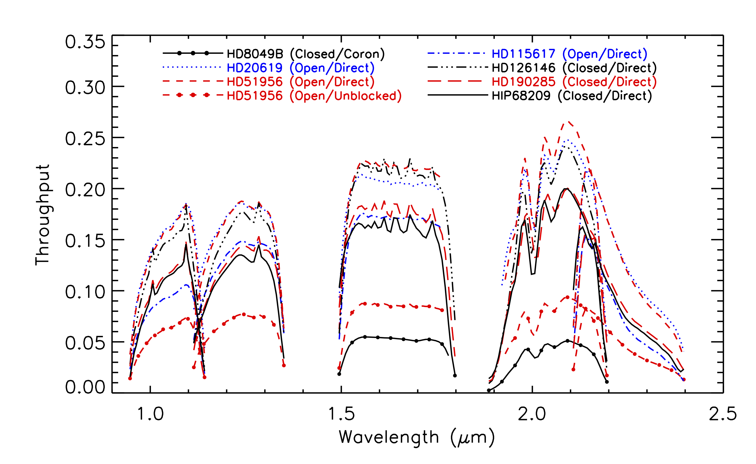
Figure 4: The throughput of the GPI instrument, the Gemini telescope and the atmosphere of the Earth measured using seven calibration targets observed during the GPI commissioning runs (see Table 2). The different targets are differentiated by linestyle, with filled circle symbols denoting observations taken in either Unblocked mode (HD 51956) or Coron mode (for HD 8049 B).

Table 3: Average throughput measurements for Direct observations at central wavelength of each filter

Filter	Central Wavelength	Throughput
	($\mu$m)	(without coronagraph)
$Y$	1.05	$0.137\pm 0.027$
$J$	1.24	$0.166\pm 0.023$
$H$	1.65	$0.195\pm 0.025$
$K1$	2.05	$0.206\pm 0.025$
$K2$	2.26	$0.089\pm 0.025$

The average throughput measured at the central wavelength of each filter for the observations taken in the Direct mode is given in Table 3. While consistent throughput measurements are seen for targets observed on the same night (e.g. HD 20619/HD 51956) and during the same run (e.g. HD 190285/HIP 68209), there is a $\sim$30% variation in the measured throughput over the six-month period for which data are available. The cause of this variation is uncertain. The observations were all obtained under good atmospheric conditions, although gray extinction from light cloud cover above the observatory could induce a significant change in the measured throughput at certain wavelengths.

6 Ongoing development of datacube assembly algorithms

The individual lenslet PSFs are not Nyquist sampled by the detector, having FWHM between $\sim$$1.5-1.8$ pixels [39]. It is possible to slightly improve the spectral resolving power by taking into account of the micro-lens PSF extent in the datacube extraction process. We report here a second GPI DRP primitive for datacube extraction, “Assemble Spectral Datacube using mlens PSF”, that uses a model of the micro-lens PSF to disentangle the flux variations along each spectrum. This primitive has been implemented in the GPI DRP since November 2012 but is undergoing improvements. The primitive utilizes the GPI Data Simulation Tool[24] to construct a set of micro-lens PSFs calculated by taking into account the size and shape of the individual micro-lens and the modulation transfer function (MTF) of the detector pixels. The PSFs are sampled at the spatial resolution of the detector, and calculated for each spectral channel and for each PSF center sub-pixel location. Figure 5 (left) illustrates how the simulated 1.5$\mu m$ micro-lens PSF changes as the central location is shifted by a fifth of a pixel in each direction.

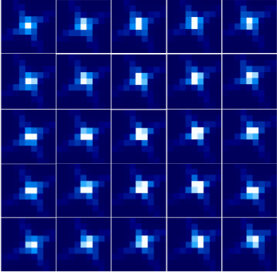
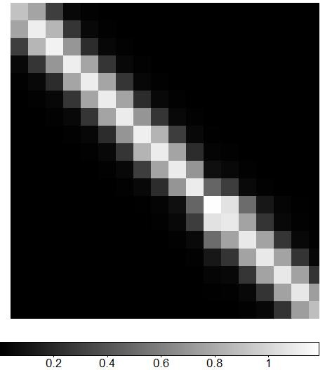
Figure 5: Left: The same simulated micro-lens PSF at $1.5\mu m$ as seen on the detector, sampled differently due to 25 different sub-pixel center locations. Just the center of the 64$\times$64 PSF is represented. Right: Example of the $(\mathbb{P}^{\prime}\mathbb{P})$ matrix to be inverted. The system is well conditioned as the matrix is almost diagonal.

The intensity $I$ of a detector pixel at position ($x$,$y$) in the image can be considered as the sum over all $N$ spectral channels $\lambda$ of the product of the micro-lens PSF $P(x-x_{c}(\lambda),y-y_{c}(\lambda),\lambda)$ centered on $(x_{c}(\lambda),y_{c}(\lambda))$ by the flux $F(\lambda)$ of the target in this channel, such as

$$I(x,y)=\sum\limits_{\lambda=1}^{\lambda=N}F(\lambda)\times P\left(x-x_{c}(\lambda),y-y_{c}(\lambda),\lambda\right).$$ (2)

This technique aims to recover the flux of each individual spectrum while mitigating the contamination by adjacent spectral channels. A term for taking into account correlated detector noise can be added to study noise propagation, but here we treat the term as negligible since this extraction happens after the removal of correlated noise in the raw images by the pipeline.

Using Equation 2, it is then possible to form a system of equations using $M$ pixels of a specific spectrum with intensities $I_{m}(x_{m},y_{m})$ where ($m=1$,$\ldots$,$M$). Letting $x_{m}^{\prime}=x_{m}-x_{c}(\lambda)$ and $y_{m}^{\prime}=y_{m}-y_{c}(\lambda)$, this system can be expressed in a matrix form $\mathbb{I}=\mathbb{P}\cdot\mathbb{F}$ as

$$\left(\begin{array}[]{c}I_{1}\\ I_{2}\\ \vdots\\ I_{M}\end{array}\right)=\left(\begin{array}[]{cccc}P(x_{1}^{\prime},y_{1}^{\prime},\lambda_{1})&P(x_{1}^{\prime},y_{1}^{\prime},\lambda_{2})&\ldots&P(x_{1}^{\prime},y_{1}^{\prime},\lambda_{N})\\ P(x_{2}^{\prime},y_{2}^{\prime},\lambda_{1})&P(x_{2}^{\prime},y_{2}^{\prime},\lambda_{2})&\ldots&P(x_{2}^{\prime},y_{2}^{\prime},\lambda_{N})\\ \vdots&\vdots&\ddots&\vdots\\ P(x_{M}^{\prime},y_{M}^{\prime},\lambda_{1})&P(x_{M}^{\prime},y_{M}^{\prime},\lambda_{2})&\ldots&P(x_{M}^{\prime},y_{M}^{\prime},\lambda_{N})\end{array}\right)\left(\begin{array}[]{c}F(\lambda_{1})\\ F(\lambda_{2})\\ \vdots\\ F(\lambda_{N})\end{array}\right).$$ (3)

Solving this for $\mathbb{F}$ gives the standard unweighted least-squares solution[40]

$$\mathbb{F}=(\mathbb{P}^{\prime}\mathbb{P})^{-1}\mathbb{P}^{\prime}\mathbb{I}.$$ (4)

As $\mathbb{P}$ is a $M\times N$ matrix, this requires in particular that $N\leq M$, that is, the number of unknown fluxes or spectral channels is smaller than or equal to the number of detector pixels of the spectrum considered to resolve the system. The system is well conditioned; the condition number associated with this linear equation is very low since $(\mathbb{P}^{\prime}\mathbb{P})$ is almost diagonal. An example of the matrix $(\mathbb{P}^{\prime}\mathbb{P})$ is represented in Figure 5 (right), showing that this algorithm is appropriate to resolve the system. This inversion technique is applied on each spectrum individually. Different choices of pixel configuration have been tested, mainly different number of columns of pixels along the spectrum. As GPI spectra are about 18 pixels long in $H$-band, 1, 3 or 5 columns of 18 pixels can be selected to form the observed $\mathbb{I}$ vector. These columns of pixels are tilted for the spectra at the edges of the field-of-view, according to the corresponding wavelength solution.

The number of spectral channels is chosen to be slightly larger than the number of channels defined by the detector-sampling-limited effective spectral resolution, i.e 10 channels given the $\sim$1.5 pixel FWHM of the micro-lens PSF on an 18 pixel-length spectrum. We performed tests with 9, 12, 15 and 18 spectral channels using simulated flat-field images and GPI data taken during the integration and testing of the instrument (Figure 6). The flat-field images were simulated using a flat spectrum with same intensity for all micro-lenses, then datacubes were extracted using the two methods. We then measured the ratio of the standard deviation of pixel intensities in a slice of the datacubes to the mean intensity in the same slices. These ratios, 4.3% for the 3$\times$1 pixel box method and 2.9% for the inversion method, shows that the inversion method was able to extract the flux more accurately in this test. The Moiré pattern visible in the flat-field image (Figure 6, top) has been identified to come from a systematic bias in the determination of the wavelength solution, for which a new method of measurement has been developed[27]. The inversion method method can extract datacube with high fidelity, but it is more sensitive to any bias in the wavelength solution or uncorrected shifts due to flexure effect than the integration method, giving a more pronounced checkerboard pattern, as shown in Figure 6 (middle, bottom).

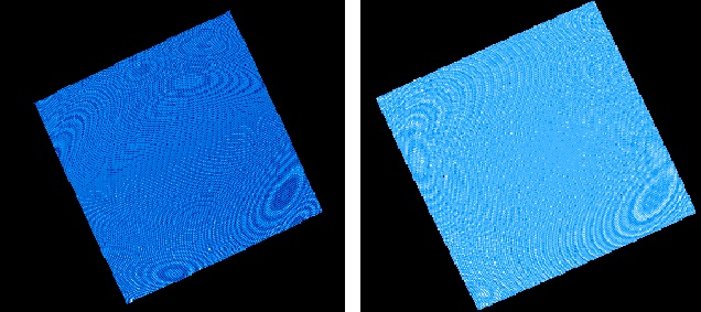
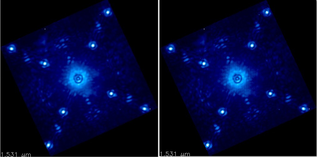
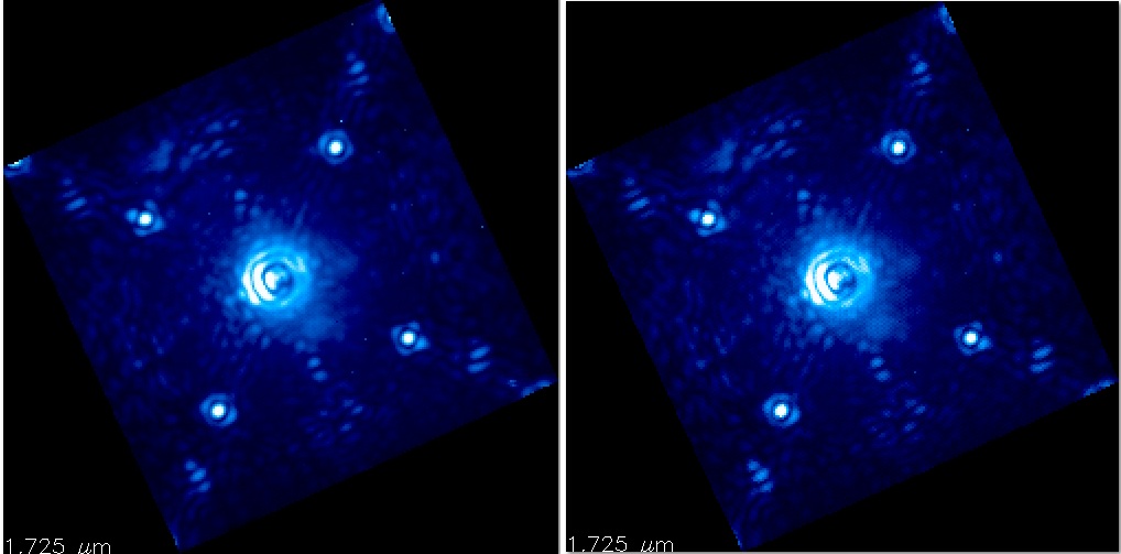
Figure 6: Comparison of images obtained by integrating the signal over a rectangular aperture along the spectra (left) and by using an inverse method taking into account the simulated micro-lens PSF (right) for GPI data taken during UCSC Integration & Test period (middle and bottom) and for simulated flat-field lamp (top).

The performance of this inversion technique is dependent upon an accurate model of the lenslet PSF. It has been demonstrated using GPI calibration data that the micro-lens PSF shape varies across the field of view[39], presenting some specific elongations for micro-lenses towards the edges of the field-of-view. This semi-empirical model of the micro-lens PSF will be implemented in a future version of the inversion technique for datacube extraction. Updated wavelength solutions[27] should also provide a significant improvement to the inversion techniques datacube output quality. This inversion method has not yet been employed much on on-sky observational data, pending these improvements. A similar technique with adaptive fitting of the flexure effects is also under development[34].

7 Conclusion & Future work

We have seen how to perform a photometry calibration to establish a relation between observed instrumental counts and expected amount of photons. On base of this calibration, all observed objects and the image itself can be transformed from counts to physical units.

We measured the throughput expressed in all filter wavebands that include the various optical components of GPI, the telescope optics as well as the transmission characteristics of the atmosphere, by using a set of known calibration stars. Throughput variability will be characterized in more details as further observations proceed.

We have seen that the pipeline can deliver high-fidelity spectrum of observed objects and provides uncertainties on this measurement. Improving the accuracy of the photometry requires to better understand all systematic errors and to optimize each step of the reduction. It could be envisaged to improve the pipeline by implementing error propagation through each step of the reduction to produce a cube giving uncertainty on each spaxel of a datacube.

Datacube extraction itself is crucial to improve the accuracy of the photometry for which we proposed a new datacube extraction method that can distangle the flux variations along each spectrum and to mitigate spectral cross-talks. Further improvements by use of empirical micro-lens PSF will be implemented.

8 Acknowledgments

The Gemini Observatory is operated by the Association of Universities for Research in Astronomy, Inc., under a cooperative agreement with the NSF on behalf of the Gemini partnership: the National Science Foundation (United States), the National Research Council (Canada), CONICYT (Chile), the Australian Research Council (Australia), Ministério da Ciéncia, Tecnologia e Inovaçāo (Brazil), and Ministerio de Ciencia, Tecnología e Innovación Productiva (Argentina). The Dunlap Institute is funded through an endowment established by the David Dunlap family and the University of Toronto.

- [1] Macintosh, B., Graham, J., Palmer, D., Doyon, R., Gavel, D., Larkin, J., Oppenheimer, B., Saddlemyer, L., Wallace, J. K., Bauman, B., Evans, J., Erikson, D., Morzinski, K., Phillion, D., Poyneer, L., Sivaramakrishnan, A., Soummer, R., Thibault, S., and Veran, J., “The Gemini Planet Imager,” in [Society of Photo-Optical Instrumentation Engineers (SPIE) Conference Series ], Proc. SPIE 6272 (jul 2006).
- [2] Poyneer, L. A., Macintosh, B. A., and Véran, J.-P., “Fourier transform wavefront control with adaptive prediction of the atmosphere,” Journal of the Optical Society of America A 24, 2645–+ (2007).
- [3] Poyneer, L. A., De Rosa, R. J., Macintosh, B., Palmer, D. W., Perrin, M. D., Sadakuni, N., Savransky, D., Bauman, B., Cardwell, A., Dillon, D., Gavel, D., Goodsell, S. J., Hartung, M., Hibon, P., Rantakyrö, F. T., Thomas, S., and Véran, J.-P., “On-sky performance during verification and commissioning of the Gemini Planet Imager’s adaptive optics system,” in [This Conference ], (2014).
- [4] Guyon, O., “A theoretical look at coronagraph design and performance for direct imaging of exoplanets,” Comptes Rendus Physique 8, 323–332 (Apr. 2007).
- [5] Sivaramakrishnan, A., Soummer, R., Oppenheimer, B. R., Carr, G. L., Mey, J. L., Brenner, D., Mandeville, C. W., Zimmerman, N., Macintosh, B. A., Graham, J. R., Saddlemyer, L., Bauman, B., Carlotti, A., Pueyo, L., Tuthill, P. G., Dorrer, C., Roberts, R., and Greenbaum, A., “Gemini Planet Imager coronagraph testbed results,” in [Society of Photo-Optical Instrumentation Engineers (SPIE) Conference Series ], Society of Photo-Optical Instrumentation Engineers (SPIE) Conference Series 7735 (July 2010).
- [6] Soummer, R., Sivaramakrishnan, A., Oppenheimer, B. R., Brenner, D., Pueyo, L., Marois, C., Macintosh, B., Graham, J. R., Palmer, D., and GPI Team, “The Gemini Planet Imager: Coronagraph Design & Testbed,” in [American Astronomical Society Meeting Abstracts ], Bulletin of the American Astronomical Society 39, #134.01 (Dec. 2007).
- [7] Konopacky, Q. M., Barman, T. S., Macintosh, B. A., and Marois, C., “Detection of Carbon Monoxide and Water Absorption Lines in an Exoplanet Atmosphere,” Science 339, 1398–1401 (Mar. 2013).
- [8] Oppenheimer, B. R., Baranec, C., Beichman, C., Brenner, D., Burruss, R., Cady, E., Crepp, J. R., Dekany, R., Fergus, R., Hale, D., Hillenbrand, L., Hinkley, S., Hogg, D. W., King, D., Ligon, E. R., Lockhart, T., Nilsson, R., Parry, I. R., Pueyo, L., Rice, E., Roberts, J. E., Roberts, Jr., L. C., Shao, M., Sivaramakrishnan, A., Soummer, R., Truong, T., Vasisht, G., Veicht, A., Vescelus, F., Wallace, J. K., Zhai, C., and Zimmerman, N., “Reconnaissance of the HR 8799 Exosolar System. I. Near-infrared Spectroscopy,” The Astrophysical Journal 768, 24 (May 2013).
- [9] Bonnefoy, M., Chauvin, G., Lagrange, A.-M., Rojo, P., Allard, F., Pinte, C., Dumas, C., and Homeier, D., “A library of near-infrared integral field spectra of young M-L dwarfs,” Astronomy & Astrophysics 562, A127 (Feb. 2014).
- [10] Marois, C., Macintosh, B., Barman, T., Zuckerman, B., Song, I., Patience, J., Lafrenière, D., and Doyon, R., “Direct Imaging of Multiple Planets Orbiting the Star HR 8799,” Science 322, 1348– (nov 2008).
- [11] Kalas, P., Graham, J. R., Chiang, E., Fitzgerald, M. P., Clampin, M., Kite, E. S., Stapelfeldt, K., Marois, C., and Krist, J., “Optical images of an exosolar planet 25 light-years from Earth,” Science 322, 1345– (nov 2008).
- [12] Lagrange, A.-M., Bonnefoy, M., Chauvin, G., Apai, D., Ehrenreich, D., Boccaletti, A., Gratadour, D., Rouan, D., Mouillet, D., Lacour, S., and Kasper, M., “A Giant Planet Imaged in the Disk of the Young Star Pictoris,” Science 329, 57– (July 2010).
- [13] Lafrenière, D., Jayawardhana, R., and van Kerkwijk, M. H., “The Directly Imaged Planet Around the Young Solar Analog 1RXS J160929.1 - 210524: Confirmation of Common Proper Motion, Temperature, and Mass,” The Astrophysical Journal 719, 497–504 (Aug. 2010).
- [14] Marois, C., Zuckerman, B., Konopacky, Q. M., Macintosh, B., and Barman, T., “Images of a fourth planet orbiting HR 8799,” Nature 468, 1080–1083 (Dec. 2010).
- [15] Macintosh, B. A., Graham, J. R., Palmer, D. W., Doyon, R., Dunn, J., Gavel, D. T., Larkin, J., Oppenheimer, B., Saddlemyer, L., Sivaramakrishnan, A., Wallace, J. K., Bauman, B., Erickson, D. A., Marois, C., Poyneer, L. A., and Soummer, R., “The Gemini Planet Imager: from science to design to construction,” in [Society of Photo-Optical Instrumentation Engineers (SPIE) Conference Series ], Proc. SPIE 7015 (jul 2008).
- [16] Graham, J. R., Macintosh, B., Doyon, R., Gavel, D., Larkin, J., Levin, M., Oppenheimer, B., Palmer, D., Saddlemyer, L., Sivaramakrishnan, A., Veran, J., Wallace, K., and Gemini Planet Imager Science Team, “Ground-Based Direct Detection of Exoplanets with the Gemini Planet Imager (GPI),” in [Bulletin of the American Astronomical Society ], Bulletin of the American Astronomical Society 38, 968–+ (dec 2007).
- [17] Macintosh, B. A., Anthony, A., Atwood, J., Barriga, N., Bauman, B., Caputa, K., Chilcote, J., Dillon, D., Doyon, R., Dunn, J., Gavel, D. T., Galvez, R., Goodsell, S. J., Graham, J. R., Hartung, M., Isaacs, J., Kerley, D., Konopacky, Q., Labrie, K., Larkin, J. E., Maire, J., Marois, C., Millar-Blanchaer, M., Nunez, A., Oppenheimer, B. R., Palmer, D. W., Pazder, J., Perrin, M., Poyneer, L. A., Quirez, C., Rantakyro, F., Reshtov, V., Saddlemyer, L., Sadakuni, N., Savransky, D., Sivaramakrishnan, A., Smith, M., Soummer, R., Thomas, S., Wallace, J. K., Weiss, J., and Wiktorowicz, S., “The Gemini Planet Imager: integration and status,” in [Society of Photo-Optical Instrumentation Engineers (SPIE) Conference Series ], Society of Photo-Optical Instrumentation Engineers (SPIE) Conference Series 8446 (Sept. 2012).
- [18] Macintosh, B., Graham, J. R., Ingraham, P., Konopacky, Q., Marois, C., Perrin, M., Poyneer, L., Bauman, B., Barman, T., Burrows, A. S., Cardwell, A., Chilcote, J., De Rosa, R. J., Dillon, D., Doyon, R., Dunn, J., Erikson, D., Fitzgerald, M. P., Gavel, D., Goodsell, S., Hartung, M., Hibon, P., Kalas, P., Larkin, J., Maire, J., Marchis, F., Marley, M. S., McBride, J., Millar-Blanchaer, M., Morzinski, K., Norton, A., Oppenheimer, B. R., Palmer, D., Patience, J., Pueyo, L., Rantakyro, F., Sadakuni, N., Saddlemyer, L., Savransky, D., Serio, A., Soummer, R., Sivaramakrishnan, A., Song, I., Thomas, S., Wallace, J. K., Wiktorowicz, S., and Wolff, S., “First light of the gemini planet imager,” Proceedings of the National Academy of Sciences (2014).
- [19] Larkin, J. E., Chilcote, J. K., Aliado, T., Bauman, B. J., Brims, G., Canfield, J. M., Dillon, D., Doyon, R., Dunn, J., Fitzgerald, M. P., Graham, J. R., Goodsell, S., Hartung, M., Ingraham, P. J., Johnson, C. A., Kress, E., Konopacky, Q. M., Macintosh, B. A., Magnone, K. G., Maire, J., McLean, I. S., Palmer, D., Perrin, M. D., Quiroz, C., Sadakuni, N., Saddlemyer, L., Thibault, S., Thomas, S. J., Vallee, P., and Weiss, J. L., “The integral field spectrograph for the gemini planet imager,” in [This Conference ], (2014).
- [20] Chilcote, J., Larkin, J. E., Perrin, M. D., Perrin, M., Maire, J., Fitzgerald, M. P., , and Doyon, R., “Performance of the integral field spectrograph for the Gemini Planet Imager,” in [Society of Photo-Optical Instrumentation Engineers (SPIE) Conference Series ], Society of Photo-Optical Instrumentation Engineers (SPIE) Conference Series 8446 (July 2012).
- [21] Konopacky, Q. M., Thomas, S. J., Macintosh, B. A., Dillon, D., Sadakuni, N., Maire, J., Marois, C., Ingraham, P. J., Marchis, F., Perrin, M. D., Graham, J. R., Wang, J. J., Morzinski, K. M., Pueyo, L. A., Chilcote, J. K., Fabrycky, D. C., Hinkley, S., Kalas, P. R., Larkin, J. E., Oppenheimer, B. R., Patience, J., Saddlemyer, L., and Sivaramakrishnan, A., “Gemini planet imager observational calibrations v: astrometry and distortion,” in [This Conference ], (2014).
- [22] Chilcote, J. K., Larkin, J. E., Maire, J., Perrin, M. D., Fitzgerald, M. P., Doyon, R., Thibault, S., Bauman, B., Macintosh, B. A., Graham, J. R., and Saddlemyer, L., “Performance of the integral field spectrograph for the Gemini Planet Imager,” in [Society of Photo-Optical Instrumentation Engineers (SPIE) Conference Series ], Society of Photo-Optical Instrumentation Engineers (SPIE) Conference Series 8446 (Sept. 2012).
- [23] Perrin, M. D., Graham, J. R., Larkin, J. E., Wiktorowicz, S., Maire, J., Thibault, S., Fitzgerald, M. P., Doyon, R., Macintosh, B. A., Gavel, D. T., Oppenheimer, B. R., Palmer, D. W., Saddlemyer, L., and Wallace, J. K., “Imaging polarimetry with the Gemini Planet Imager,” in [Society of Photo-Optical Instrumentation Engineers (SPIE) Conference Series ], Society of Photo-Optical Instrumentation Engineers (SPIE) Conference Series 7736 (July 2010).
- [24] Maire, J., Perrin, M. D., Doyon, R., Artigau, E., Dunn, J., Gavel, D. T., Graham, J. R., Lafrenière, D., Larkin, J. E., Lavigne, J.-F., Macintosh, B. A., Marois, C., Oppenheimer, B., Palmer, D. W., Poyneer, L. A., Thibault, S., and Véran, J.-P., “Data reduction pipeline for the Gemini Planet Imager,” in [Society of Photo-Optical Instrumentation Engineers (SPIE) Conference Series ], Society of Photo-Optical Instrumentation Engineers (SPIE) Conference Series 7735 (July 2010).
- [25] Perrin, M., Maire, J., Ingraham, P. J., Savransky, D., Millar-Blanchaer, M., Wolff, S. G., Ruffio, J.-B., Wang, J. J., Draper, Z. H., Sadakuni, N., Marois, C., Rajan, A., Fitzgerald, M. P., Macintosh, B., Graham, J. R., Doyon, R., Larkin, J. E., Chilcote, J. K., Goodsell, S. J., Palmer, D. W., Labrie, K., Beaulieau, M., Rosa, R. J. D., Greenbaum, A. Z., Hartung, M., Hibon, P., Konopacky, Q. M., Lafreniere, D., Lavigne, J.-F., Marchis, F., Patience, J., Pueyo, L. A., Rantakyro, F., Soummer, R., Sivaramakrishnan, A., Thomas, S. J., Ward-Duong, K., and Wiktorowicz, S., “Gemini planet imager observational calibrations i: overview of the gpi data reduction pipeline,” Society of Photo-Optical Instrumentation Engineers (SPIE) Conference Series 9147 (2014).
- [26] Ingraham, P. J., Perrin, M. D., Sadakuni, N., Ruffio, J.-B., Maire, J., Chilcote, J. K., Larkin, J. E., Marchis, F., Galicher, R., and Weiss, J., “Gemini planet imager observational calibrations ii: Detector performance and calibration,” Society of Photo-Optical Instrumentation Engineers (SPIE) Conference Series 9147 (2014).
- [27] Schuyler G. Wolff, Marshall Perrin, J. M. P. J. I. F. T. R. P. H., “Gemini planet imager observational calibrations iv: wavelength calibration and flexure correction for the integral field spectograph,” in [This Conference ], (2014).
- [28] Marois, C., Lafrenière, D., Macintosh, B., and Doyon, R., “Accurate Astrometry and Photometry of Saturated and Coronagraphic Point Spread Functions,” The Astrophysical Journal 647, 612–619 (Aug. 2006).
- [29] Sivaramakrishnan, A. and Oppenheimer, B. R., “Astrometry and Photometry with Coronagraphs,” The Astrophysical Journal 647, 620–629 (aug 2006).
- [30] Wang, J. J., Rajan, A., Graham, J. R., Savransky, D., Ingraham, P. J., Ward-Duong, K., Patience, J., Rosa, R. J. D., Bulger, J., Sivaramakrishnan, A., Perrin, M. D., Thomas, S. J., Sadakuni, N., Greenbaum, A. Z., Pueyo, L., Marois, C., Oppenheimer, B. R., Kalas, P., Cardwell, A., Goodsell, S., Hibon, P., and Rantakyrö, F. T., “Gemini planet imager observational calibrations viii: Characterization and role of satellite spots,” Society of Photo-Optical Instrumentation Engineers (SPIE) Conference Series 9147 (2014).
- [31] Pickles, A. J., “A Stellar Spectral Flux Library: 1150-25000 Å,” PASP 110, 863–878 (July 1998).
- [32] Zurlo, A., Vigan, A., Hagelberg, J., Desidera, S., Chauvin, G., Almenara, J. M., Biazzo, K., Bonnefoy, M., Carson, J. C., Covino, E., Delorme, P., D’Orazi, V., Gratton, R., Mesa, D., Messina, S., Moutou, C., Segransan, D., Turatto, M., Udry, S., and Wildi, F., “Astrophysical false positives in direct imaging for exoplanets: a white dwarf close to a rejuvenated star,” Astronomy & Astrophysics 554, A21 (June 2013).
- [33] Crepp, J. R., Johnson, J. A., Howard, A. W., Marcy, G. W., Gianninas, A., Kilic, M., and Wright, J. T., “The TRENDS High-contrast Imaging Survey. III. A Faint White Dwarf Companion Orbiting HD 114174,” Astrophysical Journal 774, 1 (Sept. 2013).
- [34] Zack Draper, Christian Marois, S. W. J.-B. R. M. P. w. t. G. t., “Gemini planet imager observational calibrations ix: Least square inversion flux extraction,” in [This Conference ], (2014).
- [35] Currie, T., Burrows, A., Madhusudhan, N., Fukagawa, M., Girard, J. H., Dawson, R., Murray-Clay, R., Kenyon, S., Kuchner, M., Matsumura, S., Jayawardhana, R., Chambers, J., and Bromley, B., “A Combined Very Large Telescope and Gemini Study of the Atmosphere of the Directly Imaged Planet, Pictoris b,” The Astrophysical Journal 776, 15 (Oct. 2013).
- [36] Rayner, J. T., Cushing, M. C., and Vacca, W. D., “The Infrared Telescope Facility (IRTF) Spectral Library: Cool Stars,” The Astrophysical Journal, Supplement 185, 289–432 (Dec. 2009).
- [37] Bohlin, R. C., “HST Stellar Standards with 1% Accuracy in Absolute Flux,” in [The Future of Photometric, Spectrophotometric and Polarimetric Standardization ], Sterken, C., ed., Astronomical Society of the Pacific Conference Series 364, 315 (Apr. 2007).
- [38] Tokunaga, A. T., Simons, D. A., and Vacca, W. D., “The Mauna Kea Observatories Near-Infrared Filter Set. II. Specifications for a New JHKL’M’ Filter Set for Infrared Astronomy,” PASP 114, 180–186 (Feb. 2002).
- [39] Ingraham, P. J., Ruffio, J.-B., Perrin, M. D., Wolff, S., Draper, Z., Maire, J., Marchis, F., and Fesquet, V., “Gemini planet imager observational calibrations iii: Empirical measurement methods and applications of high-resolution microlens psfs,” Society of Photo-Optical Instrumentation Engineers (SPIE) Conference Series 9147 (2014).
- [40] Cowan, G., [Statistical Data Analysis ], Oxford science publications, Clarendon Press (1998).