Gemini planet imager observational calibrations X: non-redundant masking on GPI

Abstract

The Gemini Planet Imager (GPI) Extreme Adaptive Optics Coronograph contains an interferometric mode: a 10-hole non-redundant mask (NRM) in its pupil wheel. GPI operates at Y, J, H, and K bands, using an integral field unit spectrograph (IFS) to obtain spectral data at every image pixel. NRM on GPI is capable of imaging with a half resolution element inner working angle at moderate contrast, probing the region behind the coronagraphic spot. The fine features of the NRM PSF can provide a reliable check on the plate scale, while also acting as an attenuator for spectral standard calibrators that would otherwise saturate the full pupil. NRM commissioning data provides details about wavefront error in the optics as well as operations of adaptive optics control without pointing control from the calibration system. We compare lab and on-sky results to evaluate systematic instrument properties and examine the stability data in consecutive exposures. We discuss early on-sky performance, comparing images from integration and tests with the first on-sky images, and demonstrate resolving a known binary. We discuss the status of NRM and implications for future science with this mode.

1 INTRODUCTION

The Gemini Planet imager is an extreme AO coronagraph [1] with a 10-hole non-redundant mask (NRM) in its pupil [2]. GPI’s extreme AO wavefront control [3, 4] uses a Shack-Hartmann wavefront sensor upstream of the coronagraph and a calibration system (CAL), a low-order wavefront sensor measuring slow tip/tilt and other modes relative to the coronagraphic focal plane mask[5, 6] (the high-order sensing capability of CAL is not active). Imaging modes using the unocculted science mirror (direct and NRM) do not allow light to pass to the CAL for these low order corrections. Commissioning the instruments has seen a series of on and off sky tests of the various imaging modes and the adaptive optics controls with and without tip/tilt corrections from the CAL system.

NRM provides interferometric resolution, to angular scales of about $\lambda/2B$, $B$ being the longest hole-pair distance, at high dynamic range ($10^{2}-10^{3}$ binary contrast routinely possible from the ground). This makes NRM a well suited technique for imaging hot planet forming regions inside young circumstellar disks with GPI. In particular, NRM is a powerful probe of gaps in transition disks that may be harboring the building blocks of planets [7, 8, 9]. GPI provides spectral information by employing an integral field unit spectrograph (IFS). Imaging in spectral mode may enable the detection of emission features associated with strong circum-planetary accretion in these regions. NRM can also operate with the imaging polarimeter [10] and may provide an eye into polarized disks at small inner working angles.

NRM images are also a diagnostic tool for the operation of the instrument and wavefront correction controls. For IFS images, NRM fringes are a sensitive measure of the pixel scale relative to the NRM mask and can provide an independent check on the wavelength calibration if the plate scale (i.e., the magnification from the telescope) is known [11]. The sensitivity of the NRM PSF, due to improved angular resolution, could also be a good tool to measure atmospheric dispersion and dispersion correction, especially in brighter sources.

2 The GPI NRM

GPI’s NRM has 10 holes that form 45 non-redundant baseline vectors. The mask is designed to provide good coverage in spatial frequencies without strong directional preference. The middle of Figure 1 shows our hole labeling convention that we will refer to throughout this paper. The right of Figure 1 shows the corresponding hole-pair baselines plotted in the Fourier plane (spatial frequencies).

Figure 1: Labeled Holes and Splodges: Left: GPI’s 10-hole NRM[12]. Center: We establish a numbering convention, which helps to keep track of hole and baseline dependent systematics and aids diagnosis of problems, shown in the center. Right: we plot the associated hole-pair baselines.

Measuring fringe phases and amplitudes from point sources is a powerful diagnostic for the instrument and provides information regarding the wavefront. The fringe stability over subsequent exposures determines performance for imaging science with NRM. Careful analysis of the fringes, both through Fourier transform diagnostics and an analytic fringe fitting can reveal the angular scale of various instrument instabilities.

In this paper we focus on the NRM observations from GPI commissioning in the context of diagnosing instrument systematics and instabilities. In Section 3 we describe how to analyze the data in Sections 4 and 5 we describe alignment procedures and observations. In Section 6 we explore the details of diagnostics NRM provides to GPI in general. Section 7 provides a demonstration of contrast and presents analysis of early contrast detection performance that will be reported more comprehensively in future communications.

Figure 2: Independent Closure Triangles: A set of 36 unique closure triangles in order of increasing perimeter. The addition of fringe phases around these closing triangles is insensitive to piston phase error in the pupil.

3 Analysis Techniques

Fringe amplitudes and phases are extracted from NRM images through Fourier principles. These fringe observables reveal information about the wavefront. The fringe amplitudes can be measured by fringe contrast and fringe phases by fringe center shift in the image. For $N$ holes there are $N(N-1)/2$ baselines. Phases measure antisymmetric structure, appropriate for detecting multiple point source objects and faint companions. Amplitudes can measure centro-symmetric structure. Measuring fringe observables may be done with a good model of the fringes that form the image, or by Fourier transforming the data, both to measure signal in spatial frequencies that correspond to mask baselines.

The closure phase is the sum of fringe phases around a closed triangle. Imaging a point source with relatively stable and unaberrated optics, this sum should be zero for all $N\choose 3$ closure triangle combination [13, 14, 15]. Figure 2 displays an example of a subset of 36 independent closure triangles, in general $(N-1)(N-2)/2$, for GPI’s mask, where all baselines are represented. Closure phases have the remarkable property of immunity to any piston phase errors located in a pupil Non-zero closure phase can be the result of structure in the image or uncorrected high order wavefront error due to atmosphere or imperfect optics. Precision in the closure phase measurement sets the limit on achievable contrast with NRM.

3.1 Analytic Fringe Fitting

We fit fringe phases with an analytic model of the NRM PSF that describes the PSF as a a sum of fringes corresponding to each hole-pair baseline [16, 17]. The NRM PSF can be represented mathematically by an envelope, $P$ (the Airy pattern for circular holes as in GPI NRM), modulated by sinusoidal fringes from each baseline. Constant pistons can be expressed as a constant phase shift in the transform of the of the pupil mask. For pupil units $\b{x}$ and image units $\b{k}$:

$$a(\b{k})a^{*}(\b{k})=P(\b{k})\sum_{i=1}^{N}\sum_{j=1}^{N}e^{-i\b{k}\cdot(\b{x}_{i}-\b{x}_{j})+i(\phi_{i}-\phi_{j})}$$ (1)

In general, relative pistons between holes contribute constant fringe phases $\Delta\phi_{i,j}$’s at hole centers $\b{x}_{i}$’s.

$$psf=P(\b{k})\{10+\cos{(\b{k}\cdot(\b{x}_{1}-\b{x}_{2}))}\cos{(\Delta\phi_{1,2})}$$

$$-\sin{(\b{k}\cdot(\b{x}_{1}-\b{x}_{2}))}\sin{(\Delta\phi_{1,2})}$$

$$+\cos{(\b{k}\cdot(\b{x}_{1}-\b{x}_{3}))}\cos{(\Delta\phi_{1,3})}$$

$$-\sin{(\b{k}\cdot(\b{x}_{1}-\b{x}_{3}))}\sin{(\Delta\phi_{1,3})}$$

$$+...\}$$ (2)

The model can be tuned to reflect plate scale, sub-pixel centering, and other similar parameters. These can be fit for in the Fourier plane. For the GPI data cubes, we consider each slice to be monochromatic in the model.

3.2 Fourier approach and diagnostic tools

We also provide an independent analysis of the data through the Fourier approach [18, 19, 20] with the aperture masking pipeline at University of Sydney. Additionally, Fourier transforming the data provides a quick and intuitive look directly at the phase and amplitude behavior with time or wavelength and can help diagnose baseline-dependent errors. Tracking down the hole pairs that contribute to phase peculiarities can help distinguish between hole-dependent errors and baseline-dependent errors, and also reveal morphological signatures in the phase.

4 Alignment in Pupil

The first thing to check when using NRM with extreme AO is mask alignment in the pupil. We determined the mask position in the pupil with a few custom poke patterns on the deformable mirror, illuminating the pupil with the internal source, imaging with the pupil viewing camera. One asymmetric set of pokes helped determine the rotation between the the MEMS plane (Figure 3) and the pupil to help map the NRM holes to actuator locations. The rotation between the poke pattern and the as-designed NRM orientation (with respect to the MEMS DM) is roughly 243.6 degrees counter-clockwise Another set confirmed a new aligned position of the mask.

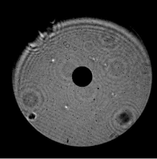
Figure 3: Left: asymmetric 5-poke pattern on the $48\times 48$ GPI MEMS actuator array. Right: The resulting pupil image. The pupil image is vignetted at the top, a result of miaslignment of the pupil-sensing camera, not the science path. The pupil viewing camera also shows other features like dust on the camera and bad actuators.

Figure 4 shows the NRM in its nominal position from the pupil viewer (a) and overlaid on a clear pupil image (b). A few holes appear to be clipped, but since the pupil viewer optics vignet the on-axis beam it is difficult to determine the edge. The secondary obstruction provided a good handle on the pupil center and which holes were cut off at the edge. We shifted the mask from the nominal position to lie entirely in the pupil. Figure 5 shows a poke pattern of NRM hole centers mapped to the deformable mirror actuators, and as seen through the mask in the pupil. A set of NRM-specific pokes (Figure 5) confirmed the new hole position mapping to the MEMS plane and confirmed our alignment. The actuators covered by each hole are obvious and can be used to track back peculiarities in the AO control. We confirm that the holes miss spiders and known dead actuator locations, as designed. The dead actuators are indicated in masked regions at the top of Figure 5.

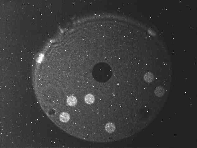
Figure 4: Left: The nominal alignment of the NRM seen with the pupil viewing camera. Holes 4 and 5 look completely cut off, hole 6 partially. Right: Pupil viewer images of the NRM and overlaid with the clear pupil show vignetting by the pupil viewing system.

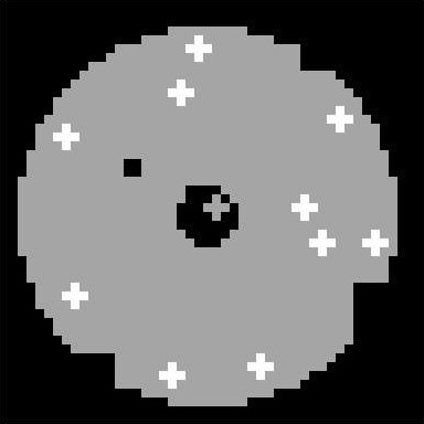
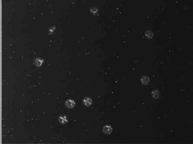
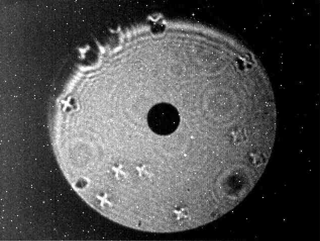
Figure 5: Top: The expected NRM hole centers (white crosses) overlaid on the bad actuator map of active subapertures (gray). Bottom left: The poke pattern seen through the mask moved to its new position. Bottom right: The poke pattern seen through the clear pupil. The NRM hole centers miss known bad actuator locations.

5 Observations

NRM observations on GPI were taken over the course of several commissioning runs. These have provided a good sample of both short exposure and longer exposure point source observations as operations changes throughout commissioning. The observations discussed in this manuscript are summarized in Table 1.

Table 1: Summary of commissioning observations discussed in this report

Month	Target description	Details	Purpose	Notes
Dec	- HR 2690 (binary)[21]	6 frames in $H$ for 60s	Performance	The first complete NRM dataset
2014	- HR 2716 (calib)	6 frames in $H$ for 60s	verification	saw long exposures that produced
	- HR 2839 (calib)	6 frames in $H$ for 60s		inconsistent phases between frames.
				Seeing was 0.6” or better.
Mar			Engineering	We aimed for shorter exposures to
2014	- HD 63852 (pt src)	20 frames $Y,H$ for 1.5s		better understand instabilities.
				Seeing was 0.6” or better.
May	Point sources			We Tested new AO control
2014	- HD 63852	20 frames in $H$ for 1.5s	Engineering &	software with short and long
	- HD 142695	8 frames in $J$ for 54s	Performance	exposures on known point sources
	- HD 142384	8 frames in $J$ for 37s	verification	used for NRM calibration [9] and took
				a sequence of short exposures with
	Internal source	60 frames in $H$ at 1.5s		the internal source. Median seeing
				was 0.8”.

6 Instrument diagnostics

We have identified the most obvious systematics in the data. These are a combination of static phase and amplitude trends and temporal instabilities that ultimately limit contrast and resolution with GPI NRM. Understanding the behavior of the instrument in NRM can help measure the instrument wavefront in static conditions (e.g. lab or internal source measurements) as well as diagnose unseen behaviors in the adaptive optics control that operates without CAL tip/tilt correction. CAL must receive light through the coronagraph hole to send to a low-order shack hartman sensor, with a 4 pixel camera (quad cell) to measure tip/tilt in the calibration system [5, 6]. All non-coronagraphic science exposures operate without this low order correction.

6.1 Static phases

We observe static piston phases in the NRM fringes during the most stable exposures in the lab (before commissioning) and with the internal source while on the telescope. Static pistons do not affect NRM contrast because they calibrate out in the closure phase calculation. However, they provide information about the instrument wavefront after AO correction. Exposures from the stable internal source (measured by analytic model fitting) match the general trend of phases measured during integration and tests in July 2013. Figure 6 shows the morphology of the fringe phases matches between July 2013 and May 2014. We plot the phases for each baseline in Figure 7 over 20 exposures in May (solid lines) compared to those recovered from July intergration and tests (dots).

Static phases seen by the NRM are measuring the wavefront inherent in the optical system, possibly caused by the non-common-path of the AO system and the imaging detector. Such wavefront error can cause quasi-static speckles that can limit the obtainable contrast of coronagraphy and conventional imaging, but calibrate out in closure phase. Knowing the static phases could potentially feed into the adaptive optics control and improve contrast in other imaging modes.

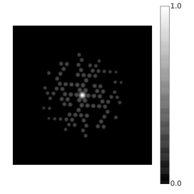
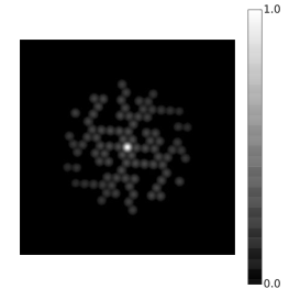
Figure 6: Top: Fringe amplitudes (Left) and phases (Right) measured from July 2013 integration and tests from an average of several exposures. Bottom: Amplitudes and phases from May 2014 internal source single exposure on telescope. Both sets of amplitudes drop with longer baselines. The phases appear morphologically similar.

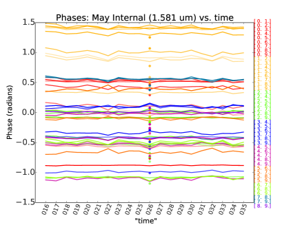
Figure 7: May 2014 internal source phases plotted over time. The single data-points correspond to average phase from July 2013 integration and tests. They are in general lower in July when the instrument was not attached to the telescope.

6.2 Wavelength dependent instabilities

December 2013 commissioning data was taken with the NRM misaligned in the pupil, so that holes 4,5, and 6 were potentially clipped by the edge of the pupil, which could contribute to decreased amplitudes in related baselines. Any wavefront error remaining after AO correction will cause wavelength dependent changes in both amplitude and phase. If there is Fresnel fringing, for example from near field vignetting in the optical path, we may also expect wavelength dependent effects. We note that odd behavior at the edges of the band in our measurements are a result of reduced filter throughput at band edges [22].

In all datasets we see the amplitudes rise with increasing wavelength (Figure 8), especially in lower average amplitude baselines, which tend to be longer. This is true even for data taken with the internal source while on the telescope and integration and test data from the lab at UCSC. The trends are relatively flat at the higher visibility amplitude baselines, and become more steeply sloped at longer baselines where wavefront error has the largest effect. The effect is more pronounced in on-sky data.

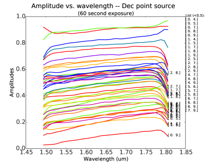
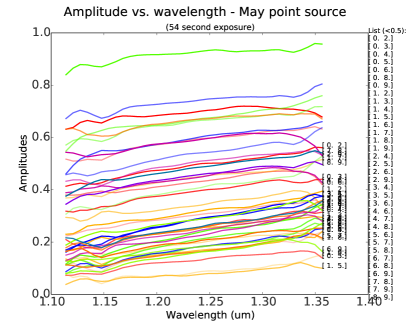
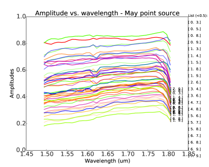
Figure 8: Average fringe amplitude over an observing sequence for each wavelength slice. Baselines [1,5] and [0,9] show up consistenly between observations. Low amplitudes at longer baselines are at least partially due to jitter in the image.

Comparing amplitudes from exposures during integration and testing to internal source exposures on the telescope shows what additional instabilities exist on the telescope from various vibrations. The rise in amplitude with longer wavelength exist in the I&T data, which also shows the lower amplitude baselines that involve holes 9 and 5 seen in many of the on-sky datasets. The effect systematically limits fringe amplitude measurements at some of the longer baselines and at shorter amplitudes. This may explain improved contrast at longer wavelengths. Currently, vibration and non-common path error are the best candidates for the source of reduced visibility amplitude at longer baselines. Residual wavefront error should scale with wavelength, just as we observe.

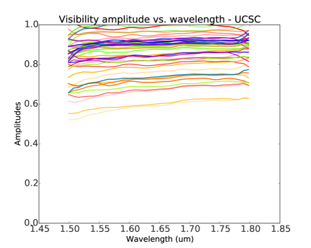
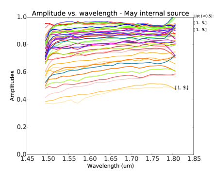
Figure 9: Visibility amplitude behavior with wavelength for an mean exposure from integration and test data (left) and the mean over a set of 20 exposures with the internal source in May. The two display a similar trend. Particular baselines show lower amplitudes and there is systematic wavelength dependence, possibly due to instrument vibrations. The amplitudes are worse while the instrument is on the telescope, which could be a result of additional vibrations.

6.3 Pointing instabilities

Data taken in December 2013 showed significant drops in amplitude, especially in some longer baselines, indicating some kind of temporal instability. In March we took a set of short exposures ($1.5$s) on point source HD 63852 to see how fringes behaved on shorter timescales. While displaying the sharpest fringes on sky, these revealed jitter in the image, within about a pixel, close to $14\mathrm{mas}$.

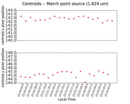
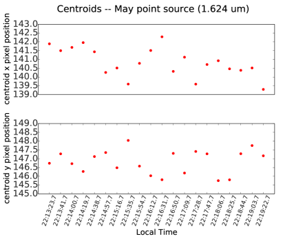
Figure 10: Image centroid position with time: Both March and May 2014 runs looked at the same point source for 1.5s exposures, approximately 20s apart. Both show some jitter in the pointing. The pointing stability appears worse for the May run, consistent with higher wind speeds and poorer observing conditions.

Instabilities in telescope pointing cause the PSF to smear during exposures, decreasing the sensitivity and obtainable contrast of all modes. NRM is particularly vulnerable, as analysis requires accurate measurement of fringes which are blurred by this effect. Pointing errors causes a change in fringe phase and a decrease in amplitude, both important quantities for NRM. This has particular impact on the ability to measure accurate interferometric visibilities on long exposures since different frames are affected to different extents, making calibration difficult. Analysis of short exposure images shows that most frames are unaffected. This indicates the frequency of jitter in on a several second timescale.

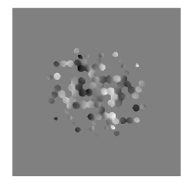
Figure 11: Image smearing from jitter: Left: the image shows smearing due to some source of motion. Center: The power spectrum shows the fringe amplitudes of the drop significantly in affected spatial frequencies (for example, compared to a more evenly filled amplitude signal in Figure 6). Right: Low fringe amplitudes in turn produce lower fringe phases signal at those spatial frequencies.

6.4 Large dynamic pistons

NRM images are sensitive to systematics not seen with the coronagraph. In the December 2013 point source images we saw fringe jumps in the data: large and sudden changes in the static wavefront error, causing a shift in fringe phase and amplitude between consecutive frames of the same source. In March we saw the same behavior return in short exposures. In the amplitudes these shifts often appeared with clipping over particular holes. The large change in fringe phases occurs in both short and long baselines.

This instability was particularly pernicious given its tendency to temporarily change the fringe visibility, making calibration difficult. There is also some evidence to suggest that the systematic closure phases were affected, also leading to poor calibration.

One convincing explanation of big fringe jumps is a buildup of phase on the tweeter DM. A rotation of the whole reference centroid pattern (e.g. due to rotation of the lenslets relative to the CCD) should be reconstructed into a flat wavefront, as no phase aberration upstream of the lenslets can produce that motion. However, the GPI reconstructor projects rotation into a wavefront aberration (concentrated at the pupil edges), due to both the Fourier Transform Reconstruction edge extension and the missing subapertures that cover MEMS bad actuators. Change in the wavefront sensor (WFS) gain changes the measured rotation of the centroids relative to the (slightly rotated) reference centroid set, producing wavefront anomalies at the pupil edge that can vary rapidly. This was mitigated in the May 2014 run by explicitly removing the rotation component of the centroids before reconstruction [4]. Figure 13 shows an example of this buildup of phase, which would contribute phase to both short and long baselines. These fringe jumps were not visible in May data, though the closure phases were in general less stable with poorer weather conditions. While more work on analyzing both the data and telemetry is required to confirm this connection, this demonstrates NRM as a tool for identifying systematics that are hard to diagnose with other modes.

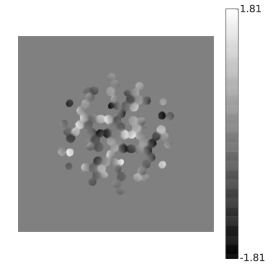
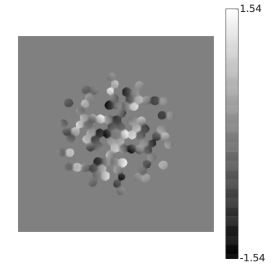
Figure 12: Top: Consecutive exposures of point source HR 2716 in December 2013. Bottom: Consecutive exposures of HD 63852 in May 2014. Both show a similar shift in fringe phases during the observing sequence.

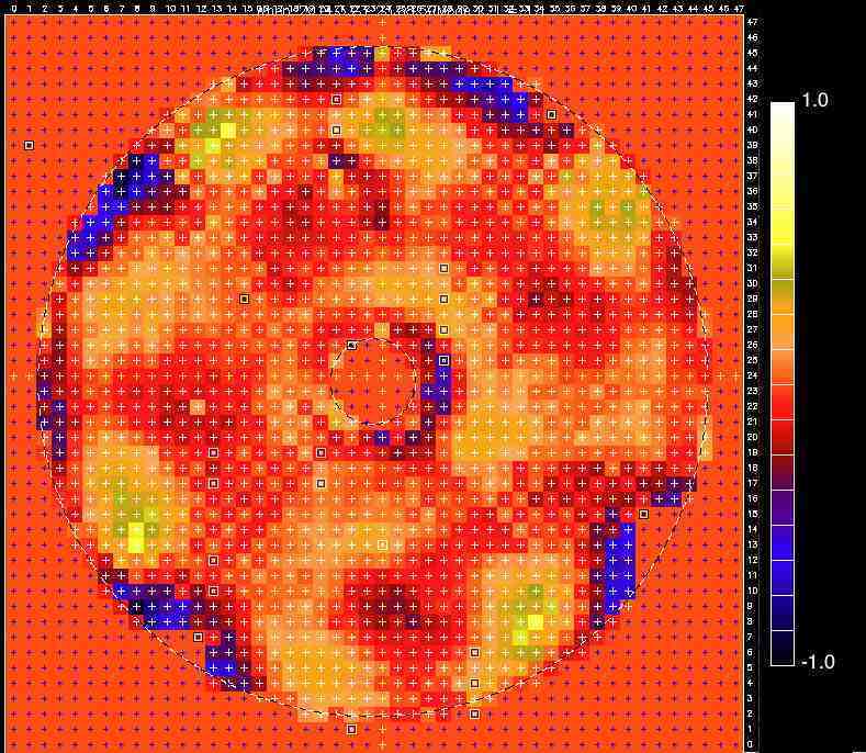
Figure 13: March 2014 Telemetry: Phase (microns) builds on the tweeter DM trying to correct rotation seen between the WFS lenslet and CCD pixels.

7 Performance

7.1 Binary detection

As a demonstration, in December we observed known binary HR 2690 in $H$ band. We recovered the companion at separation of $88.4\pm 0.5$ mas and contrast ratio of $5.94\pm 0.09$. We recovered the companion in 24 minutes of data. Section 7.2 discusses a current estimate of detection limits for short exposures.

7.2 Closure phase stability

Despite a few outstanding instabilities, GPI’s NRM is capable of high dynamic range measurements, competitive with masking modes on older instruments. In long exposures where pointing jitter smears the data, variations can be calibrated if enough data are taken. In the most stable conditions on the telescope from the internal source (without atmospheric turbulence) closure phase is stable, a median standard deviation of 0.0046 radians in $H$ band (uncalibrated). In Figure 14 we plot the closure phase error with wavelength for the internal source compared with measurements on sky in March and May 2014.

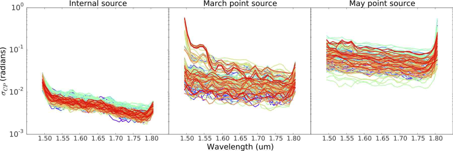
Figure 14: Perfomance: Closure phase standard deviation from internal source exposures on the telescope. Phases are very stable and predict raw contrast as low as several $\times\ 10^{3}$ for similar conditions. On sky in March closure phase error was roughly an order of magnitude higher, and in May even worse. March and December had clear conditions while May had thin and thick cirrus. We’ve reject 3 frames of visible smearing in the May dataset for this calculation.

In March 2014, short exposures saw relatively stable closure phases that had a median standard deviation $0.016$ radians, uncalibrated. These closure phases roughly follow the wavelength trend seen in July 2013 lab data [11] and in exposures with the internal source. Observing conditions were worse in May and observations saw increased pointing jitter (Figure 10). The median standard deviation in closure phase was 0.055 radians. This could be an explanation for larger error in the closure phases, decreased contrast sensitivity. In Figure 14 the three most visibly smeared frames from are not included in analysis.

Analyzing the data through the Sydney pipeline, March 2014 short exposure closure phases had a median standard deviation of $1.57$ degrees for each group of 10 frames after calibration, allowing detections of point sources at up to 6.5 magnitudes. In the 17 exposures in May 2014, calibrating the first 9 frames with the remaining frames the root-mean-square (rms) of the calibrated closure phases was 1.62 degrees. This would provide robust detections at up to 6 magnitudes. These results suggest the current performance of GPI NRM is similar to that obtained routinely with older instruments such as NIRC2 at Keck and NACO at VLT. However, the extra wavelength dimension provides more independent data per frame than is obtained with these instruments, resulting in higher contrast detection limits with the same number of frames and similar closure phase scatter.

More consistent and calibratable measurements can be made with stable pointing. When seeing and conditions are poor, it will be difficult to obtain good contrast with NRM in the current state of the instrument. Fixing image jitter will help bring contrast sensitivity closer to levels seen in the lab. We are using two independent pipelines and tracking down discrepencies in order to further understand systematics and how much we can calibrate them.

8 Discussion

As a diagnostic tool NRM can be leveraged for measuring the wavefront. Wavefront phase reconstructions can be made from fringe phases in the data. Comparison of analytic models with and without observed phases also provides a good estimate for strehl ratio calculation. This would assess the quality of the wavefront when the instrument operates without CAL corrections. In the future, NRM may also be used to test atmospheric dispersion in IFS mode, since the sub-pixel centering of the PSF is precisely measureable. With its finer resolution, NRM can also be used for plate scale calibration from known-separation binaries.

An upgrade to the real-time AO control software correction that accounts for the rotation between CCD pixels and WFS lenslets [4] appears to fix the anomalous fringe jumps seen in earlier data. While there was phase variation in May, when the new AO control software was installed and applied, this distinct phase jump was not observed. Pointing jitter appeared to be worst in May, when cloud cover, wind, and seeing were worst. This was likely the biggest source of instability. It will be difficult to understand phase systematics without fixing the pointing jitter. A good test in the future may be to take NRM exposures with reduced vibrations, when the IFS cryo-coolers are turned off, and see if there are any improvements or changes in the fringe behavior.

Even with remaining instabilities, NRM on GPI is competitive with older NRM instruments, and can additionally provide both spectral and polarimetric information. While, this analysis focued on IFS data, NRM in polarization will be a very interesting imaging mode. Solving image jitter will make amplitude measurements more stable enabling better NRM imaging of disks. NRM in polarization may be able to observe polarized disks closer in than other imaging modes. Looking at large disk gaps close in will open a new search space for GPI at the Y,J,H,K wavebands.

While NRM is demonstrating moderate contrast capability, there remain instrument systematics inhibiting better NRM performance. A trend of lower amplitudes at particular longer baselines may just be a property of the instrument, but can be manageable with a reasonable level of stability. By far the most serious factor limiting NRM performance is image jitter on sky. This reduces the contrast attainable for fainter targets that require longer exposures. While some of the effect will calibrate out, the data will lack some visibility amplitude information at longer baselines.

NRM is a very promising mode on GPI, for young star companion and disk science and also instrument calibrations and diagnostics. There are more calibration opportunities to explore with NRM, especially those that can be done with brighter targets. Improved wavefront control will make possible improved contrast detection limits as well as precision measurement on sky.

- [1] Macintosh, B., Graham, J. R., Ingraham, P., Konopacky, Q., Marois, C., Perrin, M., Poyneer, L., Bauman, B., Barman, T., Burrows, A. S., Cardwell, A., Chilcote, J., De Rosa, R. J., Dillon, D., Doyon, R., Dunn, J., Erikson, D., Fitzgerald, M. P., Gavel, D., Goodsell, S., Hartung, M., Hibon, P., Kalas, P., Larkin, J., Maire, J., Marchis, F., Marley, M. S., McBride, J., Millar-Blanchaer, M., Morzinski, K., Norton, A., Oppenheimer, B. R., Palmer, D., Patience, J., Pueyo, L., Rantakyro, F., Sadakuni, N., Saddlemyer, L., Savransky, D., Serio, A., Soummer, R., Sivaramakrishnan, A., Song, I., Thomas, S., Wallace, J. K., Wiktorowicz, S., and Wolff, S., “First light of the gemini planet imager,” Proceedings of the National Academy of Sciences (2014).
- [2] Sivaramakrishnan, A., Soummer, R., Oppenheimer, B. R., Carr, G. L., Mey, J. L., Brenner, D., Mandeville, C. W., Zimmerman, N., Macintosh, B. A., Graham, J. R., Saddlemyer, L., Bauman, B., Carlotti, A., Pueyo, L., Tuthill, P. G., Dorrer, C., Roberts, R., and Greenbaum, A., “Gemini Planet Imager coronagraph testbed results,” in [Society of Photo-Optical Instrumentation Engineers (SPIE) Conference Series ], Society of Photo-Optical Instrumentation Engineers (SPIE) Conference Series 7735 (July 2010).
- [3] Poyneer, L. A., Véran, J.-P., Dillon, D., Severson, S., and Macintosh, B. A., “Wavefront control for the Gemini Planet Imager,” Proc. SPIE 6272, 62721N–62721N–12 (2006).
- [4] Poyneer, L. A., Macintosh, B. A., Palmer, and W., D., “On-sky performance during verification and commissioning of the gemini planet imager’s adaptive optics system,” in [This Conference ], Society of Photo-Optical Instrumentation Engineers (SPIE) Conference Series 9147 (2014).
- [5] Lloyd, J. P., Oppenheimer, B. R., Digby, A. P., Newburgh, L., Brenner, D., Shara, M., Graham, J. R., Kalas, P., Perrin, M., Sivaramakrishnan, A., Makidon, R., Kuhn, J., Whitman, K., and Roberts, Jr., L. C., “The Lyot project: toward exoplanet images and spectroscopy,” in [Earths: DARWIN/TPF and the Search for Extrasolar Terrestrial Planets ], Fridlund, M., Henning, T., and Lacoste, H., eds., ESA Special Publication 539, 513–518 (Oct. 2003).
- [6] Wallace, J. K., Angione, J., Bartos, R., Best, P., Burruss, R., Fregoso, F., Levine, B. M., Nemati, B., Shao, M., and Shelton, C., “Post-coronagraph wavefront sensor for Gemini Planet Imager,” in [Society of Photo-Optical Instrumentation Engineers (SPIE) Conference Series ], Society of Photo-Optical Instrumentation Engineers (SPIE) Conference Series 7015 (July 2008).
- [7] Kraus, A. L. and Ireland, M. J., “LkCa 15: A Young Exoplanet Caught at Formation?,” ApJ 745, 5 (Jan. 2012).
- [8] Cieza, L. A., Lacour, S., Schreiber, M. R., Casassus, S., Jordán, A., Mathews, G. S., Cánovas, H., Ménard, F., Kraus, A. L., Pérez, S., Tuthill, P., and Ireland, M. J., “Sparse aperture masking observations of the fl cha pre-transitional disk,” ApJL 762, L12 (Jan. 2013).
- [9] Biller, B., Lacour, S., Juhász, A., Benisty, M., Chauvin, G., Olofsson, J., Pott, J.-U., Müller, A., Sicilia-Aguilar, A., Bonnefoy, M., Tuthill, P., Thebault, P., Henning, T., and Crida, A., “A likely close-in low-mass stellar companion to the transitional disk star hd 142527,” ApJL 753, L38 (July 2012).
- [10] Perrin, M. D., Graham, J. R., Larkin, J. E., Wiktorowicz, S., Maire, J., Thibault, S., Fitzgerald, M. P., Doyon, R., Macintosh, B. A., Gavel, D. T., Oppenheimer, B. R., Palmer, D. W., Saddlemyer, L., and Wallace, J. K., “Imaging polarimetry with the Gemini Planet Imager,” in [Society of Photo-Optical Instrumentation Engineers (SPIE) Conference Series ], Society of Photo-Optical Instrumentation Engineers (SPIE) Conference Series 7736 (July 2010).
- [11] Greenbaum, A. Z., Sivaramakrishnan, A., Pueyo, L., Ingraham, P., Thomas, S., Wolff, S., Perrin, M. D., Norris, B., and Tuthill, P. G., “Wavelength calibration and closure phases with the Gemini Planet Imager IFS using its non-redundant mask,” in [Society of Photo-Optical Instrumentation Engineers (SPIE) Conference Series ], Society of Photo-Optical Instrumentation Engineers (SPIE) Conference Series 8864 (Sept. 2013).
- [12] Lenox Laser (Glen Arm, MD).
- [13] Jennison, R. C., “A phase sensitive interferometer technique for the measurement of the Fourier transforms of spatial brightness distributions of small angular extent,” MNRAS 118, 276 (1958).
- [14] Baldwin, J. E., Haniff, C. A., Mackay, C. D., and Warner, P. J., “Closure phase in high-resolution optical imaging,” Nature 320, 595–597 (Apr. 1986).
- [15] Haniff, C. A., Mackay, C. D., Titterington, D. J., Sivia, D., and Baldwin, J. E., “The first images from optical aperture synthesis,” Nature 328, 694–696 (Aug. 1987).
- [16] Lacour, S., Tuthill, P., Amico, P., Ireland, M., Ehrenreich, D., Huelamo, N., and Lagrange, A.-M., “Sparse aperture masking at the VLT. I. Faint companion detection limits for the two debris disk stars HD 92945 and HD 141569,” A&A 532, A72 (Aug. 2011).
- [17] Greenbaum, A. Z., Pueyo, L., Sivaramakrishnan, A., and Lacour, S., “An Image-Plane Algorithm for Non-Redundantly Masked Imaging,” submitted .
- [18] Tuthill, P. G., Monnier, J. D., Danchi, W. C., Wishnow, E. H., and Haniff, C. A., “Michelson Interferometry with the Keck I Telescope,” PASP 112, 555–565 (Apr. 2000).
- [19] Lloyd, J. P., Martinache, F., Ireland, M. J., Monnier, J. D., Pravdo, S. H., Shaklan, S. B., and Tuthill, P. G., “Direct Detection of the Brown Dwarf GJ 802B with Adaptive Optics Masking Interferometry,” ApJL 650, L131–L134 (Oct. 2006).
- [20] Ireland, M. J., “Phase errors in diffraction-limited imaging: contrast limits for sparse aperture masking,” MNRAS 433, 1718–1728 (Aug. 2013).
- [21] Hartkopf, W. I., Tokovinin, A., and Mason, B. D., “Speckle Interferometry at SOAR in 2010 and 2011: Measures, Orbits, and Rectilinear Fits,” AJ 143, 42 (Feb. 2012).
- [22] Maire, J., Ingraham, P. J., Rosa, R. J. D., Perrin, M. D., Rajan, A., Savransky, D., Wang, J. J., Ruffio, J.-B., Wolff, S. G., Chilcote, J. K., Doyon, R., Graham, J. R., Greenbaum, A. Z., Konopacky, Q. M., Larkin, J. E., Macintosh, B. A., Marois, C., Millar-Blanchaer, M., Patience, J., Pueyo, L. A., Sivaramakrishnan, A., Thomas, S. J., and Weiss, J. L., “Gemini planet imager observational calibrations vi: Photometric and spectroscopic calibration for the integral field spectrograph,” in [This Conference ], Society of Photo-Optical Instrumentation Engineers (SPIE) Conference Series 9147 (2014).