ABSTRACT

The Gemini Planet Imager (GPI) is a new facility, extreme adaptive optics (AO), coronagraphic instrument, currently being integrated onto the 8-meter Gemini South telescope, with the ultimate goal of directly imaging extrasolar planets. To achieve the contrast required for the desired science, it is necessary to quantify and mitigate wavefront error (WFE). A large source of potential static WFE arises from the primary AO wavefront sensor (WFS) detector’s use of multiple readout segments with independent signal chains including on-chip preamplifiers and external amplifiers. Temperature changes within GPI’s electronics cause drifts in readout segments’ bias levels, inducing an RMS WFE of 1.1 nm and 41.9 nm over 4.44 degrees Celsius, for magnitude 4 and 11 stars, respectively. With a goal of $<$2 nm of static WFE, these are significant enough to require remedial action. Simulations imply a requirement to take fresh WFS darks every 2 degrees Celsius of temperature change, for a magnitude 6 star; similarly, for a magnitude 7 star, every 1 degree Celsius of temperature change. For sufficiently dim stars, bias drifts exceed the signal, causing a large initial WFE, and the former periodic requirement practically becomes an instantaneous/continuous one, making the goal of $<$2 nm of static WFE very difficult for stars of magnitude 9 or fainter. In extreme cases, this can cause the AO loops to destabilize due to perceived nonphysical wavefronts, as some of the WFS’s Shack-Hartmann quadcells are split between multiple readout segments. Presented here is GPI’s AO WFS geometry, along with detailed steps in the simulation used to quantify bias drift related WFE, followed by laboratory and on sky results, and concluded with possible methods of remediation.

Keywords: adaptive optics, high contrast imaging, Gemini Planet Imager, GPI

1 Introduction

Exoplanet detection and characterization are imperative in understanding planet and planetary system formation and evolution. Currently, the majority of detection methods are indirect, limited to rough characterizations of the planet’s mass and radius. In contrast, direct imaging actually resolves and images the assumed planet’s light, allowing explicit determination of attributes such as spectra and planet-star separations, in turn establishing temperature and surface gravity, and ultimately revealing atmosphere and thermal evolution.

Recent advances in adaptive optics, the measurement and compensation of wavefront distortions through high frequency CCDs, i.e. 1 kHz frame rate, and high-order deformable mirrors, i.e. 1000 or more actuators, have made possible the development of high contrast astronomical imaging instruments. With an expected planet/star contrast ratio of 10^-6 to 10^-7 from 0.2-0.8 arcseconds of planet-star separation, and a projected sensitivity to young ($<$1GYr), Jovian-mass planets at a distance of 5-100 AU, the Gemini Planet Imager (GPI)[1] will be able to contribute greatly to the unexplored range of possible exoplanet discovery.

Understanding and quantifying sources of wavefront error within GPI, discussed here, is necessary to achieving science images capable of planet detection.

2 AOWFS

2.1 CCID-66

The Lincoln Labs CCID-66, used in the Shack-Hartmann wave front sensor (SHWFS) in the adaptive optics (AO) system, consists of 160x160 active pixels, separated into 16x64 pixel segments. The CCID-66 incorporates a planar JFET first-stage amplifier in each segment to provide on-chip gain and reduce readout noise, but this may contribute to increased drifts in bias or gain levels. For GPI’s purposes, only the central 128x128 pixels are used.

2.2 Geometry

2.2.1 128x128

The 128x128 pixel array used by the SHWFS is partitioned into 2x2 pixel blocks, called quadcells, by designating every third column and row of pixels, starting from the bottom-left side of the image, as unused bands, Figure 1a. These bands prevent light from spilling into neighboring quadcells in the case of sudden, large turbulence, hence named guard bands. The array is physically situated such that when illuminating the lenslet array, prior in the optical path, the resulting focal points hit said quadcells, and allow for centroid calculations and in turn phase reconstructions. With this configuration, the available 128x128 pixels allows a maximum 43x43 usable lenslets.
Furthermore, the array is sectioned into 16x64 pixel segments, each of which is read out by an independent signal chain including on-chip preamplifiers and external amplifiers, Figure 1a. Multiple signal chains allow for faster readout speeds albeit, in practice, introduce discontinuities among intrinsic bias levels of individual segments. This can lead to misleading centroid calculations and phase reconstructions, consequently a larger wavefront error, and ultimately issues in the science, see Section 3.

2.2.2 96x96

The read out 128x128 arrays have a stored bias frame subtracted, their guard bands removed, and are manipulated such that a 96x96 array remains consisting purely of quadcells - using the 96x96 array space, centroid and phase reconstructions are computationally more convenient. As previously stated, the SHWFS has 43 usable lenslets across, leaving zero padding around the borders, Figure 1b.

2.2.3 48x48

GPI’s wavefront Fourier-transform reconstructor (FTR) algorithm[2] converts the 96x96 array into a 48x48 array phase map. From a computational point of view, it is more convenient to produce an array of these dimensions, regardless of only using 43x43 lenslets, as it is consistent with simulations and it leaves an array large enough to add 2 rings of MEMS slaves. In steps, the centroids are computed from the 96x96 array, reference centroids are subtracted, and the phase is reconstructed.

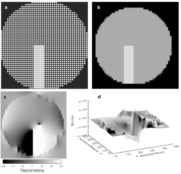
Figure 1: Major steps in the simulation are illustrated in this extreme case. a) The highlighted region shows a 30% bias drift of the original signal in one of the sixteen 16x64 pixel segments with its own readout electronics. Note the unused, single pixel bands between quadcells, known as guard bands. Also note the particular geometry results in splitting of certain quadcells among various readout segments. b) The 96x96 array after removing guard bands. Note the 4 pixel border along the bottom and left as well as the 6 pixel border along the top and right, leaving 86 valid pixels across, or 43 quadcells across, corresponding to the 43 subaperatures or lenslets across. c) The phase reconstructed in 2-D, and d) the same phase reconstructed in 3-D.

3 Bias drift

Partitioning the 128x128 space into 16x64 pixel segments allows faster readout speed through the use of multiple taps, one for each segment. As a consequence, each segment has its own intrinsic bias level, different from others’. Furthermore, each segment’s bias level fluctuates depending heavily on temperature, primarily the temperature of GPI’s electronic enclosure (EE) box containing the SHWFS electronics. This poses a problem for centroid calculations of light focused on quadcells split between readout segments; a difference in bias levels between two halves of a quadcell can be misinterpreted as a slope of the wavefront, at which point the AO will mistakenly move a DM actuator in attempt to correct for this. With a large enough temperature change, this effect could potentially induce significant WFE, Figure 2.

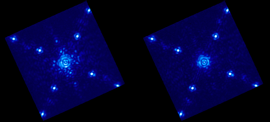
Figure 2: Showing a single wavelength channel of two different end-to-end images, one before (left) and one after (right) taking a new AO WFS dark, as well as new reference centroids. A clear improvement of the image is seen.

3.1 Simulation

In studying the effects of bias drifts through simulation, it is necessary to accurately replicate GPI’s SHWFS geometry, described in Section 2.2, to properly reconstruct meaningful centroids and phases. Starting in the 128x128 space, all pixels in all valid quadcells are assigned a specific digital number (DN). Of importance, here, is the particular DN assigned to said pixels, as bias fluctuations relative to the signal are ultimately of significance. Simulating real signals, as opposed to arbitrarily choosing DNs, is clearly more informative and thus desirable. Defined by GPI’s optics, a simple equation allows us to convert star magnitudes to DN/ms/pixel seen by the WFS,

$$DN=10^{-1[\frac{m-4}{2.5}-\log(1485)]}$$ (1)

where $m$ is the user-defined star magnitude. It follows that a dimmer star will yield less DNs and therefore a given bias change will induce relatively more WFE.

Once the star magnitude is fixed, different bias levels can be set to individual readout segments, before removing guard bands and converting to the 96x96 pixel space. Shown in Figure 1a, some quadcells are split among various readout segments - the boundaries of the readout segments are defined in the 128x128 pixel space, therefore it is crucial to apply the various bias levels here. Centroids for each quadcell in the 96x96 array are then calculated, from which the phase is reconstructed and stored in a 48x48 array. Figure 1 shows an extreme case where one readout segment’s bias increases by 30% of the signal.

It is more useful, once again, to apply real bias levels and drifts seen by GPI. Over several nights bias levels across the WFS chip were read out and recorded, in addition to numerous temperatures measured by different sensors within GPI. These biases were then applied accordingly, with different magnitude stars set as the signal, and resulting phases were reconstructed. With a 4.44^∘C change in GPI’s EE air inlet temperature over $\sim$12 hours, a maximum bias drift of 95.5 DN was seen. For a magnitude 4 star, the former effect will result in 1.074 nm RMS WFE, alternatively 0.273 nm RMS/^∘C in the linear region, justifiably adequate to leave unaccounted for.

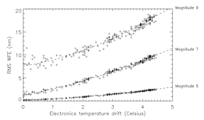
Figure 3: Showing the WFE as a function of relative temperature change. For magnitudes 5, 7, and 9 stars, a 4.44^∘C change causes 2.56, 10.02, and 18.73 nm RMS WFE, respectively.

In comparison, when observing dimmer targets this effect becomes significant enough to require correction. The same temperature change ultimately results in RMS WFEs of 9.802 nm, 14.63 nm, 18.27 nm, 23.57 nm, and 41.91 nm for magnitudes 7, 8, 9, 10, and 11 stars, respectively; correspondingly, this translates to 2.05, 2.55, 2.57, 2.40, 2.27 nm RMS/^∘C in the linear region. However, for star magnitudes $>$9 the signal seen by GPI’s WFS becomes weak enough to the point where bias drifts resulting from even fractions of a degree of temperature change become a significant percentage of the original signal, leading to a large, initial RMS WFE, Figure  4. Eventually, the bias drifts sufficiently as to exceed the original signal and reconstructed phases practically represent only bias. Therefore, to mitigate WFE, the rate at which one must update the subtracted WFS dark image increases, not only as the rate of temperature change increases, but also as the measured starlight decreases.

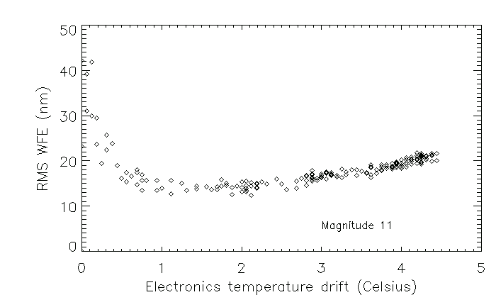
Figure 4: Showing the RMS of the WFE as a function of relative temperature change for a magnitude 11 star. Due to the weak signal, even slight variations in temperature lead to bias drifts relatively large enough to compose a significant fraction of the original signal, ultimately leading to a large, initial RMS WFE. Eventually the bias drifts sufficiently to practically overtake the signal and phase reconstructions essentially represent only bias.

3.2 On sky performance

In order to see the effects of the bias drifts on image quality on sky, the bias was intentionally allowed to drift while spectroscopic H band images were taken on GPI’s science detector[3]. After a series of images, a fresh AO WFS dark image was taken and another set of images queued. Figure 5 depicts column slices through the pair of exposures just before and after the new AO WFS dark image was taken. With an average drift of 4.59 DN on an I mag = 8.9, the peak counts in each star of the binary system HD 139498 decreased by 18.1% and 14.0% respectively; with this bias drift, simulations imply an induced static WFE of 6.64 nm RMS.

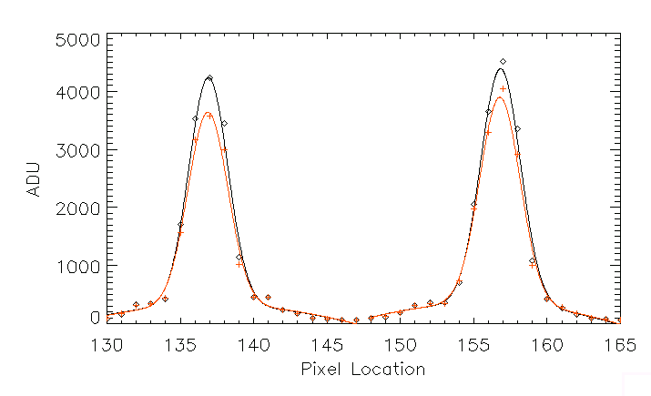
Figure 5: HD 139498 (I mag = 8.9) and its binary companion were directly imaged in H band and Gaussians were individually fit to a column slice through each star’s PSF. With an average bias drift of 4.59 DN, a decrease in peak counts of 18.1% and 14.0% are seen respectively for each star. The red plot corresponds to images that contain static WFE from AO WFS bias drifts, while the black plot corresponds to images that presumably contain little, if any, static WFE from AO WFS bias drifts, or lack thereof.

4 Methods of remediation

A method of remediation that has been implemented and tested, is the use of the unilluminated corner pixels of the WFS to track the bias drifts. The DN of each corner pixel is boxcar averaged, then averaged with each other, determining a single correction value. Said correction value is differenced from the dark value and applied to all active pixels in every frame. Figure  6 shows the effectiveness of the correction over a period of 45 minutes. However, this correction does not mitigate frame to frame fluctuations, nor does it correct for readout segment differential bias drifts. This method compensates for nondifferential bias drifts across the WFS, which also have significant effects if left uncorrected. Take, for example, centroid calculations for the simplified case of a 1-D ”quadcell” with just 2 pixels of intensities A and B:

$$CenterofGravity=\frac{(A-B)}{(A+B)}$$ (2)

If a uniform bias drift, N, is applied to the entire ”quadcell”, the measured centroid becomes:

$$CenterofGravity=\frac{(A+N)-(B+N)}{(A+N)+(B+N)}=\frac{(A-B)}{(A+B+2N)}$$ (3)

For N$>$0, the centroider will report a lower centroid, leading to underestimation of the phase and hence undercorrection. Ultimately, the AO will converge to the right solution, as it is running in closed loop, but effectively the centroid and control loop have a lower gain, therefore reducing the temporal bandwidth for correcting atmospheric turbulence. Furthermore, if a nonzero reference centroid exists that corresponds to a particular, correct actuator position/local slope, the centroider will not measure the same value at times when it should, and will have to overcorrect. Thus, this method of correction remains useful and has proven effective on sky by comparing end to end science images, Figure  7.

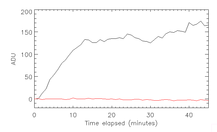
Figure 6: The unilluminated corners of the WFS are used to track the bias drifts and subtract them from active pixels. Here, an intentional temperature drift was induced, showing a clear effectiveness of the bias correction (red) compared to no bias correction (black).

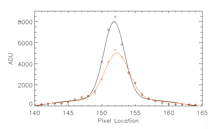
Figure 7: HD 76608 (I mag = 9.9) was directly imaged in H band and a Gaussian fit to a column slice through the PSF. With bias drift compensation turned on (black), the FWHM decreases by 17% and the peak pixel count increases by 33% compared to without bias drift compensation (red).

5 Future work

A method of remediation in consideration for the future is the use of the unilluminated top and bottom pixel rows of the CCID-66 to track the differential bias drifts. With this method it would be possible to correct the bias drifts individually for each segment. The bias drifts explained in this paper were unforeseen during design stages, thus, for increased speed, the top and bottom rows are currently not read out, and therefore this method could not yet be implemented nor tested.

6 Acknowledgements

The Gemini Observatory is operated by the Association of Universities for Research in Astronomy, Inc., under a cooperative agreement with the NSF on behalf of the Gemini partnership: the National Science Foundation (United States), the National Research Council (Canada), CONICYT (Chile), the Australian Research Council (Australia), Ministerio da Ciencia, Tecnologia e Inovacao (Brazil), and Ministerio Innovacion Productiva (Argentina). We acknowledge financial support of the Gemini Observatory, the Center for Adaptive Optics at UC Santa Cruz (NSF AST-9876783), the NSF (AST-0909188; AST-1211562), NASA Origins (NNX11AD21G; NNX10AH31G), the University of California Office of the President (LFRP-118057), and the Dunlap Institute, University of Toronto.

References

- [1] B. Macintosh, J. R. Graham, P. Ingraham, Q. Konopacky, C. Marois, M. Perrin, L. Poyneer, B. Bauman, T. Barman, A. S. Burrows, A. Cardwell, J. Chilcote, R. J. De Rosa, D. Dillon, R. Doyon, J. Dunn, D. Erikson, M. P. Fitzgerald, D. Gavel, S. Goodsell, M. Hartung, P. Hibon, P. Kalas, J. Larkin, J. Maire, F. Marchis, M. S. Marley, J. McBride, M. Millar-Blanchaer, K. Morzinski, A. Norton, B. R. Oppenheimer, D. Palmer, J. Patience, L. Pueyo, F. Rantakyro, N. Sadakuni, L. Saddlemyer, D. Savransky, A. Serio, R. Soummer, A. Sivaramakrishnan, I. Song, S. Thomas, J. K. Wallace, S. Wiktorowicz, and S. Wolff, “First light of the gemini planet imager,” Proceedings of the National Academy of Sciences , 2014.
- [2] L. A. Poyneer, D. T. Gavel, and J. M. Brase, “Fast wave-front reconstruction in large adaptive optics systems with use of the Fourier transform,” Journal of the Optical Society of America A 19, pp. 2100–2111, Oct. 2002.
- [3] J. E. Larkin, J. K. Chilcote, T. Aliado, B. J. Bauman, G. Brims, J. M. Canfield, D. Dillon, R. Doyon, J. Dunn, M. P. Fitzgerald, J. R. Graham, S. Goodsell, M. Hartung, P. Ingraham, C. A. Johnson, E. Kress, Q. M. Konopacky, B. A. Macintosh, K. G. Magnone, J. Maire, I. S. McLean, D. Palmer, M. D. Perrin, C. Quiroz, N. Sadakuni, L. Saddlemyer, S. Thibault, S. J. Thomas, P. Vallee, and J. L. Weiss, “The integral field spectrograph for the gemini planet imager,” [This Conference] , 2014.