Energy-Delay Tradeoffs of Virtual Base Stations
With a Computational-Resource-Aware
Energy Consumption Model

Abstract

The next generation (5G) cellular network faces the challenges of efficiency, flexibility, and sustainability to support data traffic in the mobile Internet era. To tackle these challenges, cloud-based cellular architectures have been proposed where virtual base stations (VBSs) play a key role. VBSs bring further energy savings but also demands a new energy consumption model as well as the optimization of computational resources. This paper studies the energy-delay tradeoffs of VBSs with delay tolerant traffic. We propose a computational-resource-aware energy consumption model to capture the total energy consumption of a VBS and reflect the dynamic allocation of computational resources including the number of CPU cores and the CPU speed. Based on the model, we analyze the energy-delay tradeoffs of a VBS considering BS sleeping and state switching cost to minimize the weighted sum of power consumption and average delay. We derive the explicit form of the optimal data transmission rate and find the condition under which the energy optimal rate exists and is unique. Opportunities to reduce the average delay and achieve energy savings simultaneously are observed. We further propose an efficient algorithm to jointly optimize the data rate and the number of CPU cores. Numerical results validate our theoretical analyses and under a typical simulation setting we find more than 60% energy savings can be achieved by VBSs compared with conventional base stations under the EARTH model, which demonstrates the great potential of VBSs in 5G cellular systems.

I Introduction

The next generation (5G) cellular network has been attracting research efforts from both academia and industry. The requirements and challenges can be summarized as follows. First, it is estimated that 5G needs to support 1000 times increase in traffic capacity [1]. With limited spectrum and energy, it is challenging for cellular systems to increase the spectral efficiency and energy efficiency to cope with the huge traffic demand. Second, 5G is expected to support massive connections including not only human-to-human connections but also machine-to-machine connections. Some of them demand high data rate, while others have loose capacity requirement but require real time response and high reliability. Hence, the cellular network must be flexible enough to adapt to different connections with different characteristics. Besides, with the influence of innovative applications from IT companies, the average revenue per user of network operators tends to increase slowly or even decrease in some cases, while the expenditures increase rapidly [2]. Such trend imposes a great challenge to the sustainability of the cellular network.

Facing these challenges, conventional cellular architectures can hardly support the 5G systems for the following reasons. First, in conventional cellular architectures, resources are commonly provisioned according to peak traffic requirement. While this approach ensures quality of service (QoS), it inevitably wastes a lot of resources in realistic networks where data traffic is highly dynamic. Second, conventional base stations (BSs) manage each cell in a distributed manner. The lack of BS cooperation results in inflexibility, and makes it difficult to utilize coordinated multi-point communications (CoMP) and coordinated BS sleeping to increase the spectral efficiency and energy efficiency. Moreover, conventional BS is a complicated system where hardware and software are tightly coupled, so operators cannot easily upgrade it, nor deploy value added services quickly. To sum up, it is difficult for conventional cellular architectures to tackle the challenges faced by 5G including efficiency, flexibility, and sustainability. Therefore it is crucial to renovate cellular network architectures to meet the requirements of 5G systems.

One of the promising architecture evolution trends is integrating cloud computing technology into cellular networks. Wireless Network Cloud (WNC) [3] proposed by IBM researchers and CRAN [2] proposed by China Mobile share the same idea of moving base band units (BBUs) of BSs to a centralized cloud computing platform, and only leaving remote radio heads (RRHs) in the front end. With the help of open IT platforms, cellular systems can be more flexible and sustainable. The deployment of CRAN also demonstrates its capability to reduce the cost and improve radio access performance. Based on the existing research, we have proposed CONCERT [4], which stands for CONvergence of Cloud and cEllulaR sysTems. Its main features are heterogeneous physical resources, logically centralized resource virtualization, and software defined services. They altogether allow CONCERT to support 5G cellular systems and provide innovative services.

In cloud-based cellular network architectures, virtualization technology is vital to make BSs software defined, that is to make them virtual base stations (VBSs). The main advantage compared with conventional BSs is that computational resources such as the number of CPU cores and the CPU speed of VBSs are pooled and can be dynamically allocated to each VBS to adapt to the dynamics of the traffic demand over time and space, which brings further energy savings. However, computational resource dynamics are not captured in the existing BS energy consumption models [5, 6]. Therefore we propose a new model to assist the research, which, to our best knowledge, is the first computational-resource-aware energy consumption model for VBSs.

Energy-delay tradeoffs of BSs in wireless systems have been studied in many literatures. It was pointed out that when taking practical concerns into account, the energy-delay tradeoff deviates from the simple monotonic curve [7]. Our previous work analyzed the energy-delay tradeoffs of conventional BSs with the EARTH energy consumption model [8, 9]. In this paper we analyze the energy-delay tradeoff relationship of VBSs with a computational-resource-aware model considering BS sleeping and state switching cost. Moreover, we investigate the impact of computational resources on the relationship, and compare the energy saving performance of VBSs in cloud-based architectures with EARTH BSs in conventional cellular networks to show the energy saving gain of VBSs.

The main contributions of the paper are as follows.

1. We propose a computational-resource-aware energy consumption model for VBSs which can capture the total energy consumption and reflect the dynamic allocation of computational resources.

2. We derive the explicit form of the optimal data transmission rate which minimizes the weighted sum of power consumption and average delay, and find the condition under which the energy optimal rate exists. This property indicates the opportunity to reduce the average delay and save energy simultaneously.

3. We investigate the impact of computational resources on energy-delay tradeoffs of VBSs and propose an efficient algorithm to optimize the data rate and the number of CPU cores jointly.

The rest of this paper is organized as follows. We first present our computational-resource-aware energy consumption model in Section II. Then we describe the system model in Section III. Theoretical analyses of energy-delay tradeoffs are given in Section IV. We show our numerical results in Section V and then conclude the paper in Section VI.

II Energy Consumption Model

II-A EARTH Model

The EARTH energy consumption model of BSs [5] has been widely adopted in the literature to analyze the energy efficiency of cellular systems. It has the form as:

$$P_{\text{in}}=\begin{cases}N_{\text{TRX}}P_{0}+\Delta_{\text{p}}P_{\text{out}},&0<P_{\text{out}}\leq P_{\text{max}}\\ N_{\text{TRX}}P_{\text{sleep}},&P_{\text{out}}=0\end{cases}$$ (1)

where $P_{\text{in}}$ is the total power supply of the BS, and $P_{\text{out}}$ is the output power per antenna measured at the input of the antenna element. $N_{\text{TRX}}$ is the number of antennas at the BS, $P_{0}$ is the power consumption at the minimum non-zero load, $\Delta_{\text{p}}$ is the slope of load varying power consumption, and $P_{\text{sleep}}$ is the energy consumption in sleep mode.

This model cannot be directly used with VBSs for two reasons. One is that multiple BBUs reside in one cloud infrastructure, so the energy consumption of BBU per BS should be reduced. The other is that by virtualization, the base band computational resources can be dynamically allocated, and the BBU application can be run only when necessary. However, the EARTH model cannot reflect the variations of computational resources. As a result, a new model for VBSs under cloud-based cellular architectures is required.

II-B Computation Resource Aware Model

Based on the analysis of the existing energy consumption model, we propose a computational-resource-aware energy consumption model for VBSs. Following the component based methodology of the EARTH model, we calculate the power consumption of the BBU and the RRH in the VBS separately, and take the summation as the total power consumption:

$$P=P_{\text{R}}+P_{\text{B}}$$ (2)

where $P_{\text{R}}$ and $P_{\text{B}}$ are the power consumption of the RRH and the BBU respectively.

Regarding the RRH part, we leverage the intermediate result from the EARTH model [5]:

$$P_{\text{R}}=\frac{P_{\text{out}}}{\eta}+P_{\text{RF}}$$ (3)

where $\eta$ denotes the power amplifier (PA) efficiency, and $P_{\text{RF}}$ denotes the power consumption of the radio frequency (RF) circuits.

As for the BBU part, we calculate the energy consumption as follows:

$$P_{\text{B}}=N_{\text{c}}(P_{\text{Bm}}+\Delta_{P_{\text{B}}}\rho_{\text{c}}s^{\beta})$$ (4)

where

$$\Delta_{P_{\text{B}}}=(P_{\text{BM}}-P_{\text{Bm}})/s_{0}^{\beta},$$ (5)

$N_{\text{c}}$ denotes the number of active CPU cores, $P_{\text{Bm}}$ and $P_{\text{BM}}$ are the minimum and maximum power consumption of each core, $\rho_{\text{c}}$ denotes the CPU load by the BBU process for $N_{\text{c}}$ cores which is usually expressed in percentage, $s$ is the CPU speed, $s_{0}$ is the reference CPU speed, and $\beta$ is the exponential coefficient of CPU speed. In this model the power consumption of the BBU is linear with the number of CPU cores as well as the CPU load [10, 11]. With speed-scaling, the dynamic part of the power consumption is polynomial with the CPU speed besides the CPU load [12].

Furthermore, we capture the relationship between the utilized computational resources and the software tasks which compute samples for wireless communications. The CPU load can be expressed by the following equation:

$$\rho_{\text{c}}=\frac{f(r)}{N_{\text{c}}s}=\frac{c_{0}+\kappa r}{N_{\text{c}}s}$$ (6)

where $f(r)$ is the actual instructions per unit time and $N_{\text{c}}s$ represents the maximum instructions available per unit time. We assume $f(r)$ is linear with the data transmission rate $r$, where $c_{0}$ and $\kappa$ are relevant coefficients. The assumption is based on the profiling result in CloudIQ [13] which shows a linear relationship between the processing time of an LTE subframe and the modulation and coding scheme (MCS) used as well as the physical resource blocks (PRB) available.

Substitute (6) into (4), we get

$$P_{\text{B}}=N_{\text{c}}P_{\text{Bm}}+\Delta_{P_{\text{B}}}c_{0}s^{\beta-1}+\Delta_{P_{\text{B}}}\kappa rs^{\beta-1}$$ (7)

which means the computational power consumption is linear with the data rate.

In summary, the power consumption of a VBS is:

$$P=\begin{cases}P_{\text{B}}+P_{\text{R}},&0<P_{\text{out}}\leq P_{\text{max}}\\ P_{\text{sleep}},&P_{\text{out}}=0\end{cases}$$ (8)

III System Model

We consider one VBS on a server with $N_{\text{c}}$ active CPU cores with speed $s$. We model the system as an M/G/1 Processor Sharing (PS) queue. Traffic flows arrive at the BS with average rate $\lambda$, and each flow has an average file size $L$. The data transmission rate is $r$ $\mathrm{b}\mathrm{p}\mathrm{s}$ when the queue has customers; otherwise it is zero. So the traffic load of the queue is $\rho=\lambda L/r$. According to queueing theory, the average queue length is:

$$\mathbb{E}\{n\}=\frac{\rho}{1-\rho}=\frac{\lambda L}{r-\lambda L}$$ (9)

By applying Little’s Law, we know the average delay is $\mathbb{E}\{D\}=\mathbb{E}\{n\}/\lambda$.

In our model the VBS will go to sleep when there is no customer in the queue (“off” state), and be back to work when a new customer arrives (“on” state). In an on-off cycle, we let $T_{\text{a}}$ denote the time duration in the busy period, $T_{\text{s}}$ the time in the consecutive idle period, and $T_{\text{c}}=T_{\text{a}}+T_{\text{s}}$ the total time. We assume a switching cost $E_{\text{sw}}$ is incurred during each on-off state switching, so the average power consumption in a cycle is as follows:

$$\mathbb{E}\{P\}=p_{\text{active}}(P_{\text{B}}+P_{\text{R}})+p_{\text{sleep}}P_{\text{sleep}}+\frac{2E_{\text{sw}}}{\mathbb{E}\{T_{\text{c}}\}}$$ (10)

where $p_{\text{active}}=\rho$ and $p_{\text{sleep}}=1-\rho$ are the fraction of time of busy and idle period during one cycle respectively.

As for the cell coverage, we adopt the standard 3GPP propagation model. The radius of cell is $R$. We consider large scale path loss while ignoring shadowing loss. The downlink signal-to-interference-plus-noise ratio (SINR) is given by:

$$\text{SINR}(d)=gP_{\text{out}}=\frac{P_{\text{out}}}{L(d)FN_{0}W}$$ (11)

where $L(d)$ is the path loss, $F$ is the noise factor of the user equipment (UE), $N_{0}$ is the noise spectral density, and $W$ is the system bandwidth. For explicit analysis, we assume all users are located at the cell edge, so the overall channel gain $g$ is the same for each user. Therefore the sum data rate at the BS can be expressed by the following equation:

$$r=W\log_{2}(1+gP_{\text{out}})$$ (12)

The optimization problem is as follows:

$$\min_{r,N_{\text{c}}}\quad z=\mathbb{E}\{P\}+\alpha\mathbb{E}\{n\}$$ (13)

We want to minimize the system cost $z$, which is a weighted sum of average power consumption and average queue length. $\alpha$ is the weighting factor. The decision variables are the data rate $r$ and the number of CPU cores $N_{\text{c}}$.

IV Energy-Delay Tradeoffs

To get the optimal solution to the above problem, we first let $\frac{\partial z}{\partial r}=0$, and find that the optimal rate $r^{*}$ satisfies:

$$\Omega\left(\frac{\alpha g\eta}{\mathrm{e}}\left(\frac{r^{*}}{r^{*}-\lambda L}\right)^{2}+\frac{g\eta P_{\text{s}}-1}{\mathrm{e}}\right)=\frac{r^{*}\ln 2}{W}-1$$ (14)

where

$$P_{\text{s}} =P_{\text{o}}-P_{\text{sleep}}-2\lambda E_{\text{sw}},$$ (15)

$$P_{\text{o}} =N_{\text{c}}P_{\text{Bm}}+\Delta_{P_{\text{B}}}c_{0}s^{\beta-1}+P_{\text{RF}},$$ (16)

and $\Omega(\cdot)$ is the principal branch of Lambert W function. As $r$ increases, the left side of Eqn. (14) decreases and the right side increases. Therefore the optimal rate $r^{*}$ is unique.

We have the following proposition on the energy-delay tradeoff relationship of VBSs with varying data rate $r$.

Proposition 1

For the relationship between average power consumption and average delay, we have:

1. There exists the unique energy optimal rate $r_{\text{e}}^{*}$ when the following condition is satisfied:

   $$\lambda <\frac{P_{\text{o}}-P_{\text{sleep}}}{2E_{\text{sw}}},$$ (17)

   $$L <\frac{W}{\lambda\ln 2}\left[\Omega\left(\frac{g\eta P_{\text{s}}-1}{\mathrm{e}}\right)+1\right]$$ (18)

   The corresponding energy optimal rate is given by:

   $$r_{\text{e}}^{*}=\frac{W}{\ln 2}\left[\Omega\left(\frac{g\eta P_{\text{s}}-1}{\mathrm{e}}\right)+1\right].$$ (19)

2. When the above condition is not satisfied, the average power consumption is monotonically decreasing with the average delay.

3. In both cases, when the average delay goes to infinity, the average power consumption approaches $P_{\text{o}}+\kappa\Delta_{P_{\text{B}}}s^{\beta-1}\lambda L+\frac{2^{\frac{\lambda L}{W}}-1}{g\eta}$ .

The proof is omitted for brevity.

Remark: When the energy optimal point exists, average delay can be traded off for energy savings only when $r>r_{\text{e}}^{*}$, and when $r<r_{\text{e}}^{*}$ we can reduce the average delay and save energy simultaneously. Interestingly, the proposition has the same mathematical structure as that in our previous work [9], and for VBSs the energy optimal rate is not affected by the part of computational power consumption that is linear with data rate. The reason is that the effect of that part of computational power consumption is neutralized by time fraction factor influenced by traffic load which is inversely proportional to the data rate.

Further we investigate the impact of computational resources, in particular the impact of the number of CPU cores. On one hand, if we fix the number of CPU cores, it sets the maximum supportable rate:

$$r_{\text{M}}(N_{\text{c}})=\frac{N_{\text{c}}s-c_{0}}{\kappa}$$ (20)

On the other hand, we have $\frac{\partial z}{\partial N_{\text{c}}}=P_{\text{Bm}}>0$, $\frac{\partial r^{*}}{\partial N_{\text{c}}}>0$, which means increasing the number of CPU cores will increase the system cost and the optimal rate.

Based on the above analyses, we propose an efficient algorithm in Fig. 1 to find the optimal data rate and number of CPU cores $(r^{*},N_{\text{c}}^{*})$ jointly. In the algorithm, we search through the zone of average delay decreasingly. At first only one CPU core is considered. When the current number of CPU core cannot support the local optimal rate under that number, we mark the maximum supportable rate as one candidate of global optimal solution, and consider one more CPU core. When we find the number of CPU cores under which the local optimal rate can be achieved, we can mark the local optimal rate as the final candidate and exit the search since the total cost always increases afterwards. At last the global optimal rate and number of CPU cores can be obtained by comparing all the candidates. In this way it is unnecessary to exhaustively search all the possible numbers of CPU cores and make comparisons, which makes the algorithm efficient.

1:  Set $N_{\text{cM}}$, $N_{\text{c}}\leftarrow 1$, $S\leftarrow\Phi$

2:  while $N_{\text{c}}\leq N_{\text{cM}}$ do

3:     $\hat{r}(N_{\text{c}})\leftarrow\operatorname{argmin}_{r}z(r,N_{\text{c}})$

4:     if $\hat{r}(N_{\text{c}})\leq r_{\text{M}}(N_{\text{c}})$ then

5:        $S\leftarrow S\cup\{(\hat{r}(N_{\text{c}}),N_{\text{c}})\}$

6:        Break out of the loop

7:     else

8:        $S\leftarrow S\cup\{(r_{\text{M}}(N_{\text{c}}),N_{\text{c}})\}$

9:        $N_{\text{c}}\leftarrow N_{\text{c}}+1$

10:     end if

11:  end while

12:  return  $(r^{*},N_{\text{c}}^{*})=\operatorname{argmin}_{(r,N_{\text{c}})\in S}z(r,N_{\text{c}})$

Figure 1: The algorithm to find the optimum $(r^{*},N_{\text{c}}^{*})$. $N_{\text{cM}}$ is the maximum number of CPU cores in practical systems. $S$ is the set to store the candidates of optimal points. $\Phi$ is the empty set.

V Numerical Results

In this section we present the numerical results to show the energy-delay tradeoffs of VBSs. The simulation parameters of VBSs are listed in Table I. Among them the base band parameters are based on commodity servers, and the cellular parameters are from LTE R11 standard. As for the conventional BS under the EARTH model, we set $P_{0}=$84\text{\,}\mathrm{W}$,\Delta_{\text{p}}=2.8,P_{\text{sleep}}=$56\text{\,}\mathrm{W}$$, and $N_{\text{TRX}}=1$.

Fig. 2 shows the energy saving performance of VBSs compared with BSs under the EARTH model. We can find more than 60% energy consumed by conventional BSs can be saved when using VBSs. For example when $\lambda=$1\text{\,}\mathrm{s}^{-1}$$, about 64% savings can be achieved with the same average delay $\mathbb{E}\{D\}=$0.26\text{\,}\mathrm{s}$$ that optimizes the power consumption of conventional BSs. The savings come from traffic aware computational power consumption. The BBU power consumption scales with the actual data rate, rather than stays static in conventional BSs.

Fig. 3 shows the relationship between average power consumption and average delay given different numbers of CPU cores. For example when $N_{\text{c}}=4$, there exists the unique optimal point to minimize the energy consumption. To the right of the optimal point, there is the opportunity to reduce the average delay and achieve energy savings simultaneously. In addition, the impact of the number of CPU cores on energy-delay tradeoffs is presented in the figure. The left end points of the curves for smaller numbers of CPU cores mark the maximum supportable data rate. Given the average delay, increasing the number of CPU cores will increase the average power consumption as well as the energy optimal rate.

When both the data rate and the number of CPU cores are adjusted, the energy-delay tradeoff relationship between the average power consumption and the average delay is shown with different traffic load in Fig. 4. Note each curve is divided into several zones due to the impact of the number of CPU cores. The algorithm to find the optimum $(r^{*},N_{\text{c}}^{*})$ can be illustrated by the figure. Take the red curve with cross markers as an example. We need to compare the rightmost turning point with $\mathbb{E}\{D\}=$0.89\text{\,}\mathrm{s}$$ and the local optimal point with $\mathbb{E}\{D\}=$0.34\text{\,}\mathrm{s}$$ to determine the global optimal solution. Besides, Fig. 4 depicts the impact of traffic arrival on the energy-delay tradeoff. Either larger arrival rate or larger average file size will increase the average power consumption given average delay. The power consumption when average delay approaches infinity is monotonically increasing with $\lambda L$. Specially the two curves in the middle with the same $\lambda L$ approach the same asymptotic value.

TABLE I: Simulation parameters

CPU speed ($s$)	$2\text{\,}\mathrm{G}\mathrm{H}\mathrm{z}$
Reference CPU speed ($s_{0}$)	$2\text{\,}\mathrm{G}\mathrm{H}\mathrm{z}$
Maximum power per CPU core ($P_{\text{BM}}$)	$20\text{\,}\mathrm{W}$
Minimum power per CPU core ($P_{\text{Bm}}$)	$5\text{\,}\mathrm{W}$
Exponential coefficient of CPU speed ($\beta$)	2
Constant coefficient of instruction speed ($c_{0}$)	$7\times 10^{8}$
Rate varying coefficient of instruction speed ($\kappa$)	35
Carrier frequency ($f$)	$2\text{\,}\mathrm{G}\mathrm{H}\mathrm{z}$
Cell radius ($R$)	$0.5\text{\,}\mathrm{k}\mathrm{m}$
UE noise figure ($F$ in $\mathrm{d}\mathrm{B}$)	$9\text{\,}\mathrm{d}\mathrm{B}$
Noise spectral density ($N_{0}$)	$-174\text{\,}\mathrm{d}\mathrm{B}\mathrm{m}\mathrm{/}\mathrm{H}\mathrm{z}$
System bandwidth ($W$)	$20\text{\,}\mathrm{M}\mathrm{H}\mathrm{z}$
RF circuit power ($P_{\text{RF}}$)	$12.9\text{\,}\mathrm{W}$
PA efficiency ($\eta$)	31.1%
VBS sleeping power ($P_{\text{sleep}}$)	$6.45\text{\,}\mathrm{W}$
Switch cost ($E_{\text{sw}}$)	$5\text{\,}\mathrm{J}$

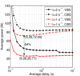
Figure 2: Power consumption comparison between the VBS and the conventional BS (CBS). $L=$2\text{\,}\mathrm{M}\mathrm{B}$$.

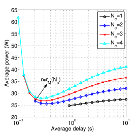
Figure 3: Energy-delay tradeoff with different numbers of CPU cores $N_{\text{c}}$.
$\lambda=$1\text{\,}\mathrm{s}^{-1}$,L=$2\text{\,}\mathrm{M}\mathrm{B}$$.

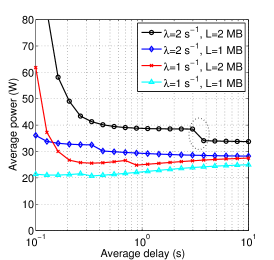
Figure 4: Energy-delay tradeoff with different arrival rates.

VI Conclusion

In this paper we propose a computational-resource-aware energy consumption model for VBSs in cloud-based cellular network architectures, and investigate the energy-delay tradeoffs of a VBS considering BS sleeping. We give the explicit form of the optimal data rate, and find the property which can depict the opportunity to achieve energy savings and reduce the average delay simultaneously. We further investigate the impact of computational resources and propose an efficient algorithm to jointly optimize the data rate and the number of CPU cores. Numerical results validate our theoretical analyses and reveal that more than 60% energy savings can be brought by VBSs compared with conventional BSs under the EARTH model. Future work will consider the multi-BS scenario.

References

- [1] 4G Americas, “Meeting the 1000x challenge: The need for spectrum, technology and policy innovations,” White Paper, Oct. 2013.
- [2] China Mobile Research Institute, “C-RAN: The road towards green RAN,” White Paper, Dec. 2013, version 3.0.
- [3] Y. Lin, L. Shao, Z. Zhu, Q. Wang, and R. Sabhikhi, “Wireless network cloud: Architecture and system requirements,” IBM Journal of Research and Development, vol. 54, no. 1, pp. 4:1–4:12, 2010.
- [4] J. Liu, T. Zhao, S. Zhou, Y. Cheng, and Z. Niu, “CONCERT: A cloud-based architecture for next-generation cellular systems,” 2014, submitted to IEEE Wireless Commun. Mag.
- [5] G. Auer, V. Giannini, C. Desset, I. Godor, P. Skillermark, M. Olsson, M. A. Imran, D. Sabella, M. J. Gonzalez, O. Blume et al., “How much energy is needed to run a wireless network?” IEEE Wireless Commun. Mag., vol. 18, no. 5, pp. 40–49, Oct. 2011.
- [6] R. Gupta, E. Calvanese Strinati, and D. Kténas, “Energy efficient joint DTX and MIMO in cloud radio access networks,” in 2012 IEEE 1st Int. Conf. Cloud Networking (CLOUDNET), 2012, pp. 191–196.
- [7] Y. Chen, S. Zhang, S. Xu, and G. Y. Li, “Fundamental trade-offs on green wireless networks,” IEEE Commun. Mag., vol. 49, no. 6, pp. 30–37, Jun. 2011.
- [8] J. Wu, Y. Wu, S. Zhou, and Z. Niu, “Traffic-aware power adaptation and base station sleep control for energy-delay tradeoffs in green cellular networks,” in Proc. 2012 IEEE Global Communications Conf. (GLOBECOM), Dec. 2012, pp. 3171–3176.
- [9] J. Wu, S. Zhou, and Z. Niu, “Traffic-aware base station sleeping control and power matching for energy-delay tradeoffs in green cellular networks,” IEEE Trans. Wireless Commun., vol. 12, no. 8, pp. 4196–4209, Aug. 2013.
- [10] M. Blackburn, “Five ways to reduce data center server power consumption,” The Green Grid Association, White Paper, Apr. 2008. [Online]. Available: http://www.thegreengrid.org/Global/Content/white-papers/Five-Ways-to-Save-Power
- [11] A. Vasan, A. Sivasubramaniam, V. Shimpi, T. Sivabalan, and R. Subbiah, “Worth their watts? - an empirical study of datacenter servers,” in Proc. IEEE 16th Int. Symp. High Performance Computer Architecture (HPCA), Jan. 2010.
- [12] K. Son and B. Krishnamachari, “SpeedBalance: Speed-scaling-aware optimal load balancing for green cellular networks,” in Proc. IEEE INFOCOM, 2012, pp. 2816–2820. [Online]. Available: http://hph16.uwaterloo.ca/~bshihada/F12-344/papers/SpeedBalanceCamera.pdf
- [13] S. Bhaumik, S. P. Chandrabose, M. K. Jataprolu, G. Kumar, A. Muralidhar, P. Polakos, V. Srinivasan, and T. Woo, “CloudIQ: A framework for processing base stations in a data center,” in Proc. 18th Annu. Int. Conf. Mobile Computing and Networking (Mobicom ’12), Istanbul, Turkey, 2012, pp. 125–136.