The Physical Parameters of the Retired A Star HD 185351

Abstract

We report here an analysis of the physical stellar parameters of the giant star HD 185351 using Kepler short-cadence photometry, optical and near infrared interferometry from CHARA, and high-resolution spectroscopy. Asteroseismic oscillations detected in the Kepler short-cadence photometry combined with an effective temperature calculated from the interferometric angular diameter and bolometric flux yield a mean density, $\rho_{\star}=0.0130\pm 0.0003$ $\rho_{\odot}$ and surface gravity, $\log{g}=3.280\pm 0.011$. Combining the gravity and density we find $R_{\star}=5.35\pm 0.20$ $R_{\odot}$ and $M_{\star}=1.99\pm 0.23$ $M_{\odot}$. The trigonometric parallax and CHARA angular diameter give a radius $R_{\star}=4.97\pm 0.07$ $R_{\odot}$. This smaller radius, when combined with the mean stellar density, corresponds to a stellar mass $1.60\pm 0.08$ $M_{\odot}$, which is smaller than the asteroseismic mass by 1.6–$\sigma$. We find that a larger mass is supported by the observation of mixed modes in our high-precision photometry, the spacing of which is consistent only for $M_{\star}\gtrsim 1.8$ $M_{\odot}$. Our various and independent mass measurements can be compared to the mass measured from interpolating the spectroscopic parameters onto stellar evolution models, which yields a model-based mass $M_{\star,\rm model}=1.87\pm 0.07$ $M_{\odot}$. This mass agrees well with the asteroseismic value, but is 2.6–$\sigma$ higher than the mass from the combination of asteroseismology and interferometry. The discrepancy motivates future studies with a larger sample of giant stars. However, all of our mass measurements are consistent with HD 185351  having a mass in excess of 1.5 $M_{\odot}$.

1. Introduction

HD 185351 ($=$ KIC 8566020, HR 7468, HIP 96459) is the third brightest target star in the field of view of the NASA Kepler Mission (Koch et al., 2010; Basri et al., 2005; Brown et al., 2011). With a Kepler-band magnitude $K_{P}=5.034$ ($V=5.18$), only CH Cyg and $\theta$ Cyg are brighter. Having exhausted its core hydrogen fuel source HD 185351 has evolved away from the main sequence and now resides at the base of the red giant branch of the H–R diagram. The Hipparcos catalog lists $B-V=0.928$, absolute V-band magnitude $M_{V}=2.13$ and a parallax-based distance of $40.83\pm 0.36$ pc (Perryman et al., 1997; van Leeuwen, 2007). The Keenan & McNeil (1989) catalog of revised MK spectral types classifies HD 185351 as a G8.5 III, indicating a giant luminosity class. However, it’s location in the observational H–R diagram is consistent with being a class IV subgiant according to the conventions used by Sandage et al. (2003), and it is among the “subgiant” targets of the Doppler-based planet survey of Johnson et al. (2006) and Johnson et al. (2011).

Recent spectroscopic analyses give mass estimates ranging from 1.4–1.7 $M_{\odot}$ (Allende Prieto & Lambert, 1999; Wang et al., 2011), indicating that HD 185351 was once an F– or A–type dwarf similar to Procyon or Sirius while on the main sequence—a massive, evolved class of stars that Johnson et al. (2007) termed the “retired A stars.” However, these and other mass estimates for single stars are based on stellar evolution models, which may contain systematic errors due to, e.g., uncertainties in the treatment of convection and errors related to the assumption of local thermodynamic equilibrium (LTE) in modeling their stellar spectra. Indeed, the mass estimates of subgiants in particular have recently been called into question based on theoretical grounds (Lloyd, 2011, 2013), and on the basis of comparing the galactic space motions of evolved and unevolved stars of various masses (Schlaufman & Winn, 2013). These studies suggest that, in a statistical sense, subgiants with masses in excess of 1.5 $M_{\odot}$ should be rare in the Solar Neighborhood. Following this argument, stars like HD 185351 are much more likely to be the evolved counterparts of G– or F–type stars, with masses in the range 1.1–1.3 $M_{\odot}$, rather than the elder brethren of A–type stars.

The resolution of this question has important implications for the reliability of stellar evolution models along the subgiant and giant branches. The issue also impacts our understanding of planet occurrence as a function of stellar mass because much of what is known about planets around stars with $M_{\star}$ $\gtrsim 1.3$ $M_{\odot}$ comes from Doppler surveys of evolved stars (e.g. Frink et al., 2002; Sato et al., 2003; Hatzes et al., 2003; Johnson et al., 2007; Niedzielski et al., 2007). This is because main-sequence A– and F–type dwarfs are rapid rotators and exhibit large amounts of radial velocity “jitter,” making the detection of even Jovian-mass planets difficult or impossible (Galland et al., 2005). However, once these stars evolve off of the main sequence, they experience rapid spin-down due to the onset of surface convective layers, which generate magnetic dynamos that carry angular momentum via stellar winds to the Alfvèn point (e.g. Gray & Nagar, 1985; do Nascimento et al., 2000).

Surveys of massive, evolved stars have discovered giant planets orbiting evolved stars with masses in excess of $\approx 1.4$ $M_{\odot}$ at rates that are much higher than have been found for solar-mass and M-type dwarf stars, revealing an apparent correlation between stellar mass and giant planet occurrence (Johnson et al., 2007; Lovis & Mayor, 2007; Johnson et al., 2010; Bowler et al., 2010). This relationship has provided important clues about the planet formation process (Laughlin et al., 2004; Kennedy & Kenyon, 2008) and hinted at fertile hunting grounds for additional planets via, e.g., high-contrast, direct imaging of main-sequence A-type stars (Marois et al., 2008; Lagrange et al., 2010; Crepp & Johnson, 2011; Nielsen et al., 2013). However, the reality of the apparent correlation between stellar mass and giant planet occurrence hinges on accurate knowledge of the masses of evolved stars (Lloyd, 2013; Johnson et al., 2013).

In the present work we address this question using several independent and complementary methods to measure the mass of the putative retired A star, HD 185351. Our methodology is similar to the study of the physical properties of the planet-hosting giant stars $\iota$ Draconis and $\beta$ Geminorum (Zechmeister et al., 2008; Baines et al., 2011; Hatzes et al., 2012). We take advantage of the proximity of HD 185351 to the Sun and its relatively large physical size ($R_{\star}\approx 5$ $R_{\odot}$) to measure its angular diameter using optical and near infrared (NIR) interferometry (see e.g. Boyajian et al., 2013). We also leverage the star’s placement in the Kepler field to measure its surface gravity and mean density based on its p-mode oscillation spectrum using Kepler short-cadence photometry. Using asteroseismic scaling relations extrapolated from the Sun, as has been done for evolved stars by, e.g., Huber et al. (2013), we obtain accurate and precise measurements of the stellar mass and radius. We then fit spectra to the star’s broad-band spectral energy distribution, along with the interferometric angular diameter, to derive the star’s effective temperature. Finally, we compare these independently-measured physical properties to the quantities estimated from the interpolation of the star’s spectroscopic properties onto stellar evolution model grids.

2. Observations and Analysis

2.1. Spectroscopy

The relative radial velocity of HD 185351 has been monitored at high precision ($\sigma_{\rm RV}\approx 5$ m s^-1) over the past decade as part of the Doppler survey of subgiants performed by Johnson et al. (2006), initiated at the Lick Observatory in Northern California using the Hamilton Spectrometer. The radial velocities of the target stars in this survey are measured with respect to co-added, iodine-free “template” spectra (Johnson et al., 2006). These template spectra are also useful for measuring the spectroscopic properties of the targets stars. Our Lick template spectra were observed with a resolving power $R=\lambda/\Delta\lambda\approx 50,000$, and a signal-to-noise ratio, S/N $\approx 130$ at 550 nm. In addition to the two Lick/Hamilton template spectra of HD 185351, we also obtained three additional templates using the HIgh Resolution Echelle Spectrometer (HIRES) on the Keck 10-meter telescope atop Mauna Kea in Hawaii (Vogt et al., 1994). Our Keck/HIRES template spectra have $R\approx 55,000$ and S/N $\approx 240$ at 550 nm.

We derived the global spectroscopic parameters from our high-resolution spectra using an iterative version of the Spectroscopy Made Easy (SME) analysis package (Valenti & Piskunov, 1996; Valenti & Fischer, 2005) which uses the Yonsei-Yale model grids (Y2; Demarque et al., 2004) to provide a constraint on surface gravity (cf Figure 1 of Valenti et al., 2009, for a illustrative flow chart of the iterative scheme). This process helps to break the degeneracies between $\log{g}$, $T_{\rm eff}$, and [Fe/H] (Torres et al., 2012). The line list used in the analysis is from Valenti & Fischer (2005) and includes the Mg b triplet region in addition to spectral segments spanning $\approx 150$ Å between 6000 Å and 6200 Å.

The spectra are first analyzed with surface gravity, effective temperature, projected rotational velocity, overall metallicity [M/H], and five elemental abundances (Na, Si, Ti, Fe, and Ni) as free parameters. Solar values are used for initial parameters except for $T_{\rm eff}$ and $\log{g}$ where rough estimates are derived from the star’s B-V color. SME uses forward modelling of the selected spectral region and $\chi^{2}$ minimization to find the best model. The Hipparcos distance and the bolometric correction for the star are used to determine $L_{\star}$ and combined with the spectroscopic $T_{\rm eff}$, [Fe/H], and [Si/Fe] (as a proxy for [$\alpha$/Fe]) to interpolate in the Y² evolution grid. If the spectroscopic and model-grid gravities don’t agree to within 0.001 dex, the gravity is fixed to that of the grid and the SME analysis is run again. This process iterates until the surface gravity of the LTE fit converges to the prediction of the evolution models.

Our SME analysis results in a metallicity [Fe/H] $=+0.16\pm 0.03$, surface gravity $\log{g}=3.31\pm 0.06$, and effective temperature $T_{\rm eff}$ $=5016\pm 44$ K. The other spectroscopic parameters are summarized in Table 1. Note that the errors are the formal uncertainties derived from the SME fitting procedure as described by Valenti & Fischer (2005), and as such do not include various unknown systematic contributions. We find that fixing the surface gravity at a value $0.03$ dex lower than our best-fitting value (the difference between our SME-based $\log{g}$ and the value measured from interferometry in § 2.4) results in a 9 K lower effective temperature, and a 0.04 dex lower metallicity. Valenti & Fischer (2005) identify a possible 0.05 dex systematic error in metallicity from SME, which will affect stellar mass estimates based on interpolating stellar evolution model grids. A systematic error of this size results in a $\pm 0.05$ $M_{\odot}$ change ($\sim 2$%) in the mass measured from model grids. Thus, systematic uncertainties of the same magnitude as our internal errors do not have a large affect on our mass measurements that rely on our SME-based spectroscopic properties.

2.2. CHARA Interferometry

We obtained long-baseline, optical/near-infrared (NIR) interferometric observations of HD 185351 using the Center for High Angular Resolution Astronomy (CHARA) Array located at Mount Wilson Observatory, near Los Angeles, CA. The CHARA Array consists of six 1-meter telescopes in a Y-configuration joined together in a central location on the observatory grounds. The longest available baseline is 330 m, making it the largest effective aperture in the world at optical and NIR wavelengths.

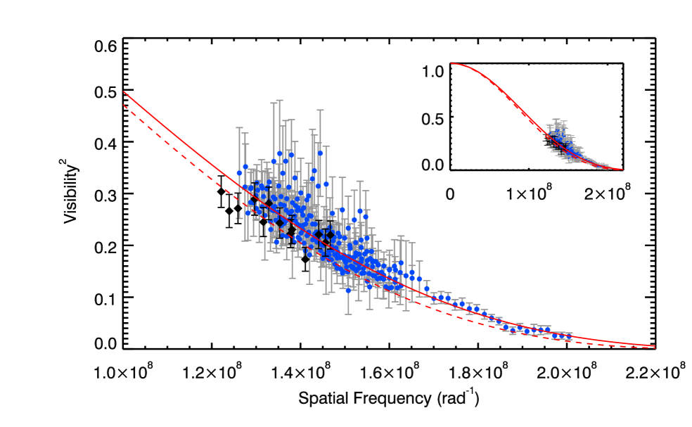
Figure 1.— Visibility versus spatial frequency. Black diamonds are measurements made with CHARA Classic, blue circles are from PAVO. The red lines show the fitted limb-darkened model to the combined data. The dashed line is for $\mu=0.32\pm 0.04$ (Classic), and the solid line is for $\mu=0.64\pm 0.03$ (PAVO). The inset shows the visibility curve over a wider scale.

We use a combination of both the CHARA Classic (ten Brummelaar et al., 2005) and Precision Astronomical Visible Observations (PAVO) beam combiners (Ireland et al., 2008). The CHARA Classic instrument is a pupil-plane beam combiner operating in NIR $J$, $H$, and $K^{\prime}$ bands in either two– or three–telescope configurations (Sturmann et al., 2010), and can observe objects as faint as $K^{\prime}\approx 9.5$. The PAVO instrument is also a three-beam pupil-plane beam combiner, operating over a wavelength range of 0.65–0.80 $\mu$m (Ireland et al., 2008, approximately the Bessell $R$-band), and has a limiting magnitude of $R\lesssim 8$.

The available angular resolution of an interferometer is dependent on the baseline as well as the wavelength. Thus, at a fixed baseline the PAVO instrument has higher angular resolution compared to Classic owing to the shorter observed wavelengths. However, in practice it is typical to configure the Array depending on the instrument and choice baseline configuration in order to sample the spatial frequencies and UV space appropriate for the science target. If the goal is to measure a diameter of a symmetric object such as HD 185351, we ensure proper sampling of the visibility curve given observations with longer baselines in the NIR with Classic and shorter baselines in the visible with PAVO. If resolution is not a necessity, it is advantageous for observations to be made in the infrared where limb-darkening corrections and their associated uncertainties are relatively small compared to those at optical wavelengths.

Both PAVO and Classic are routinely used to measure sub-milliarcsecond (mas) angular diameters of stars (Bazot et al., 2011; Derekas et al., 2011; Huber et al., 2012; Maestro et al., 2013; White et al., 2013; Boyajian et al., 2013; von Braun et al., 2011a, b, 2012, 2014). Calibrated visibilities have shown excellent agreement with measurements from various interferometers using independent beam combiners operating in the visible or near infrared (White et al., 2013; Boyajian et al., 2012b).

Our CHARA Classic observations were obtained in August of 2012 using the S2-W1 pair of telescopes, which have a maximum baseline of $B_{\rm max}=249.4$ m in $H$-band ($\lambda=1.67\mu$m; ten Brummelaar et al., 2005). Our PAVO observations were obtained on August 11, 2012, July 7, 2013, and April 6–7, 2014 with the W1-W2 pair of telescopes ($B_{\rm max}=107.9$ m), and on April 10 2014 with the E2-W2 pair of telescopes ($B_{\rm max}=156.3$ m), in 23 independent wavelength channels between $0.65-0.8$ nm. A log of the observations can be found in Table 2, where we list the UT date, interferometer configuration, number of bracketed observations, and the calibrator stars observed.

We follow the same observing procedures outlined in Boyajian et al. (2012a, b, 2013), which we briefly summarize herein. The science star was observed in bracketed sequences along with calibrators stars. Calibrators were chosen to be unresolved sources that lie within a few degrees on the sky to the science target. In order to select suitable calibrators, we use the SearchCal tool developed by the JMMC Working Group (Bonneau et al., 2006, 2011). We investigate each calibrator for any unexpected variance by comparing the data with the other calibrators observed on each night and found none. Observations were collected over the course of several nights, rotating between selected calibrators in order to reduce any night-to-night systematics, though we did not identify any evidence of systematic errors within the data set. The August 2012 PAVO observations were taken with only one calibrator, HD 188665, which has previously been tested and used as a good calibration source with PAVO observations of Kepler stars in the field (White et al., 2013).

To measure the angular diameter of HD 185351 we fitted a limb-darkened disk model to the calibrated visibility measurements (Hanbury Brown et al., 1974),

$$V = \left(\frac{1-\mu_{\lambda}}{2}+\frac{\mu_{\lambda}}{3}\right)^{-1}$$ (1)

$$\times \left[(1-\mu_{\lambda})\frac{J_{1}(x)}{x}+\mu_{\lambda}\left(\frac{\pi}{2}\right)^{1/2}\frac{J_{3/2}(x)}{x^{3/2}}\right],$$

where $V$ is the visibility, and $\mu_{\lambda}$ is the linear limb-darkening coefficient. $J_{n}(x)$ is the $n^{\mathrm{th}}$ order Bessel function, and is a function of $x=\pi\theta_{\mathrm{LD}}B\lambda^{-1}$, where $B$ is the projected baseline, $\theta_{\mathrm{LD}}$ is the angular diameter after correction for limb-darkening, and $\lambda$ is the wavelength at which the observations was made. The quantity $B\lambda^{-1}$ is also known as the spatial frequency. The linear limb-darkening coefficients were determined in $H$ and $R$ bands by interpolating the model grid by Claret & Bloemen (2011) to the spectroscopic measurements of [Fe/H], $\log{g}$ and $T_{\rm eff}$ given in § 2.1. We note that the uncertainties in the limb-darkening coefficients are small compared to the total uncertainty in the angular diameter (Huber et al., 2012; von Braun et al., 2014). Furthermore, oblateness due to rotation is expected to have negligible influence for a slowly rotating evolved star such as HD 185351.

The model–fitting procedure and parameter uncertainty estimation was performed using the method outlined in Derekas et al. (2011), which involves Monte Carlo simulations taking into account uncertainties in the data, wavelength calibration, calibrator sizes and limb-darkening coefficients. A simultaneous fit was made to the Classic and PAVO observations, with a common angular diameter and different limb-darkening coefficients. Figure 1 shows the observed visibilities and fitted model. We find HD 185351 has a limb-darkened angular diameter of $\theta_{\mathrm{LD}}=1.132\pm 0.012$ mas. Combined with the Hipparcos parallax, this measurement implies a linear radius of $R_{\star}$ $=4.97\pm 0.07$ $R_{\odot}$(corresponding to the Rosseland, or mean, radiating surface of the star). Fitting the Classic and PAVO observations individually provides consistent results (see Table 3).

2.3. SED Fitting

In order to determine HD 185351’s effective temperature and luminosity as directly as possible we perform a stellar spectral energy distribution (SED) fit to literature broad-band and spectro-photometric data published in Argue (1963, 1966); Häggkvist & Oja (1966); Mermilliod (1986); Jennens & Helfer (1975); Rufener (1976); Beichman et al. (1988); Cutri et al. (2003); McClure & Forrester (1981); Haggkvist & Oja (1987); Golay (1972); Kornilov et al. (1991); Eggen (1968); Burnashev (1985); Smith et al. (2004); Glushneva et al. (1983). Our procedure is analogous to that of von Braun et al. (2014): we perform a $\chi^{2}$-minimization of a linearly-interpolated SED template based on the G5 III and G8 III templates from the Pickles (1998) library to the aforementioned literature photometry of HD 185351.

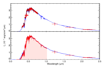
Figure 2.— Top panel: SED fit of spectral templates from the Pickles (1998) library (blue) to photometric measurements of HD 185351 from the literature (red). Horizontal bars represent the bandwidths of the photometric filters, and the vertical bars represents the literature-based uncertainties, scaled by the corresponding flux values. The 2MASS photometry is saturated for this star (Skrutskie et al., 2006), which is evident by the large photometric errors for the points beyond 1 $\mu$m. Bottom panel: SED of HD 185351 showing a HST STIS spectrum (red, $0.17-1.01\,\mu$m) and 2MASS photometry. The blue line shows the best-fitting ATLAS9 model with solar composition ([Fe/H]=0.0) and microturbulent velocity $\xi=2\,$km s^-1 (Castelli & Kurucz, 2004).

If the literature photometry values are in magnitudes, they are converted to absolute fluxes by application of published or calculated zero points. During the calculation of $\chi^{2}$ only the central broad-band filter wavelengths are correlated with the SED template’s flux value averaged over the filter transmission range in wavelength. Literature spectrophotometry data are used to trace out the shape of the SED in more detail than broadband data, and they thus help in the manual selection of the input spectral template. The SED template is scaled to minimize $\chi^{2}$ and then integrated over wavelength to obtain the bolometric flux, $F_{\rm bol}$.

In our fitting procedure, the value for interstellar reddening, $A_{V}$, is allowed to float. The best fit is obtained when $A_{V}$ is 0, which is sensible given HD 185351’s small distance. Based on 325 photometric data points, we calculate the bolometric flux to be $F_{\rm{bol,Pickles}}=2.751\pm 0.013\times 10^{-7}$ erg cm^-2 s^-1 with a $\chi^{2}_{red}=2.75$. To account for uncertainties due to the absolute flux calibration of the photometry, we added a 3% error in quadrature to the formal uncertainty, yielding $F_{\rm{bol,Pickles}}=2.751\pm 0.084\times 10^{-7}$ erg cm^-2 s^-1.

We also performed an alternative estimation of $F_{\rm{bol}}$ using a spectrum taken with the Space Telescope Imaging Spectrograph (STIS) aboard the the Hubble Space Telescope (HST). The STIS spectrum covers the $0.17-1.01\,\mu$m wavelength range at an intermediate spectral resolution of $R\sim 1000$, corresponding to $\simeq 60\,\%$ of the total radiated power of HD 185351. Potential errors induced by absolute flux calibration of ground-based spectro-photometry are reduced considerably by using this approach, as the uncertainties of the absolute flux calibration of the STIS spectrum are $\leq 1\,\%$ (Bohlin & Gilliland, 2004).

The bolometric flux is measured by fitting, through $\chi^{2}$ minimization, the STIS data to theoretical atmosphere models interpolated from a grid of ATLAS9 models with solar composition ([Fe/H]=0.0) and microturbulent velocity $\xi=2\,$km s^-1. The parameters of the model are the atmosphere temperature $T$ and $F_{\rm bol}$. Similar to the Pickles (1998) fit the best fit is found for $A_{V}=0$, as expected for such a nearby star. The bottom panel of Figure 2 shows the best-fitting model. We have confirmed the validity of the fit longward of $\lambda=1.01\,\mu$m by comparing the 2-MASS near-infrared fluxes from $J$, $H$ and $K_{s}$ broadband photometry with the fitted values. The resulting $F_{\rm bol}$ is $F_{\rm{bol,STIS}}=2.76\pm 0.04\times 10^{-7}$ erg cm^-2 s^-1, computed as the sum of the total flux of the STIS spectrum ($1.6376\pm 0.0035\times 10^{-7}$ erg cm^-2 s^-1) and the best-fit SED integrated over wavelength outside the $0.17-1.01\,\mu$m range ($1.120\pm 0.034\times 10^{-7}$ erg cm^-2 s${}^{-1})$.

Both estimates of the bolometric flux for HD 185351 are in excellent agreement. We calculate our final estimate of the bolometric flux for HD 185351 as the weighted average of $F_{\rm{bol,Pickles}}$ and $F_{\rm{bol,STIS}}$, yielding $F_{\rm{bol}}=2.758\pm 0.036\times 10^{-7}$ erg cm^-2 s^-1.

2.4. Kepler Asteroseismology

2.4.1 Background

Photometric measurements of the integrated flux from a star of sufficient precision reveal brightness oscillations from p-modes driven by stochastic convective motion near the stellar photosphere. This convective motion drives standing waves within the star characterized by spherical degree $l$ (the total number of surface nodes), azimuthal order $m$ (the number of nodes along the stellar equator), and radial order $n$ (the number of nodes from the center to the surface of the star). Modes with low $l$ and high $n$ can be observed in the stellar flux integrated over the visible stellar surface, and the nature of these modes is related to the star’s fundamental physical characteristics.

The competition between convective driving and damping in the star’s surface layers gives rise to an envelope of frequencies in the photometric power spectrum characterized by the frequency of maximum power, $\nu_{\rm max}$, and the large frequency separation, $\Delta\nu$. The latter is the average separation between power-spectrum peaks with the same value of $l$ and consecutive values of $n$. The first-order asymptotic analysis of p-mode oscillations shows that $\Delta\nu\propto\rho_{\star}^{1/2}$, where $\rho_{\star}$ is the mean stellar density (Ulrich, 1986). Scaling with respect to the Solar p-mode spectrum gives

$$\Delta\nu=\Delta\nu_{\sun}\left(\frac{M_{\star}}{M_{\odot}}\right)^{1/2}\left(\frac{R_{\star}}{R_{\odot}}\right)^{-3/2}.$$ (2)

The frequency of maximum power, $\nu_{\rm max}$, has been proposed to scale with the acoustic cut-off frequency, $\nu_{\rm ac}$, which is proportional to the inverse of the dynamical timescale or $\nu_{\rm max}\propto\nu_{\rm ac}\propto c_{s}/H_{p}$ (Brown et al., 1991; Kjeldsen & Bedding, 1995). Here, $c_{s}$ is the adiabatic sound speed in the star’s photosphere, and $H_{p}$ is the photosphere’s pressure scale height. For an ideal gas, $c_{s}\propto T^{1/2}$, where $T$ is the mean stellar temperature in the photosphere, and the scale height is given by $H_{p}\propto T/g$, where $g$ is the surface gravity. Making use of homology relations and scaling with respect to the Sun yields (Kjeldsen & Bedding, 1995; Belkacem et al., 2011):

$$\nu_{\rm max}=\nu_{\rm max,\sun}~{}\left(\frac{M_{\star}}{M_{\odot}}\right)\left(\frac{R_{\star}}{R_{\odot}}\right)^{-2}\left(\frac{T_{\rm eff}}{5777\,K}\right)^{-1/2}.$$ (3)

Equations 2 and 3 are approximate relations and require careful calibration, in particular for low-luminosity RGB stars such as HD 185351, which are significantly more evolved than the Sun. Detailed reviews of theoretical and empirical tests of asteroseismic scaling relations can be found in Belkacem (2012) and Miglio et al. (2013), and we present a brief discussion as relevant for HD 185351 here.

Empirical tests using long-baseline interferometry and Hipparcos parallaxes have shown that asteroseismic radii calculated from scaling relations are accurate to $\lesssim$4% for main-sequence and subgiant stars (Huber et al., 2012; Silva Aguirre et al., 2012). While such comparisons are currently still limited to $\sim 15\%$ for RGB stars due to poor parallax precisions, empirical tests using cluster giants (including low-luminosity RGB stars similar to HD185351) have shown agreement within $5\%$ in radius (Miglio et al., 2012b). Empirical tests of asteroseismic masses are more challenging, and have relied on eclipsing binaries and cluster members. Miglio et al. (2012b) showed that masses for RGB stars in NGC6819 show no systematic offset with a scatter of $\lesssim$ 15%, while the average asteroseismic cluster mass lies within $\sim$ 7% of the mass determined from near turn-off eclipsing binary stars (Brogaard et al., 2012).

More recently, Frandsen et al. (2013) measured the mass of an oscillating red giant in a double-lined eclipsing binary, which was found to be $\sim 10-15$% more massive than the seismic mass (Hekker et al., 2010; Huber, 2014). However, it is likely that the giant is a He-core burning red clump star, for which systematic offsets in the $\Delta\nu$ scaling relation have been noted (Miglio et al., 2012b). Additional, yet model-dependent tests can be performed by comparing properties derived from detailed modeling of individual oscillation frequencies, which contain information on the core properties of the star, such as the sound speed gradient. Such detailed modeling efforts for RGB stars have yielded radii and masses that agree within $\sim$3% and $\sim$5% of the values derived from scaling relations (Mosser et al., 2010; Di Mauro et al., 2011; Jiang et al., 2011; Huber et al., 2013).

In summary, various tests to date have shown that asteroseismic scaling relations for stars in similar evolutionary stages to HD 185351 can be expected to be accurate to $\sim 5$% and $\sim$10% in radius and mass, respectively. We note that improvements to the $\Delta\nu$ scaling relation based on models have been proposed in the literature, for example based on the comparison of $\Delta\nu$ calculated from individual frequencies with model densities (White et al., 2011), the extension of the asymptotic relation to second order (Mosser et al., 2013) or theoretical relations between fundamental properties for red giants (Wu et al., 2014). The effect of these corrections on the derived fundamental properties for HD 185351 are discussed in § 2.4.3.

2.4.2 Data Preparation

The Kepler Mission observed HD 185351 in long-cadence mode ($\approx 30$ min cadence) from Q1-3, spanning a total of roughly 200 days. However, due to the lack of a proper dedicated pixel mask, and because HD 185351 is expected to oscillate very close to the long-cadence Nyquist frequency ($\sim 300\mu$Hz), the quality of the photometry is not amenable for asteroseismology. In order to detect oscillations in HD 185351 with sufficient sampling and signal-to-noise ratio (S/N), we obtained one quarter of Kepler short-cadence data with a dedicated pixel mask through an application for Director’s Discretionary Time (DDT) in Quarter 16. The data set spans a total of 85.6 days, with a $\sim 10$ day gap during the first month due to a spacecraft safe mode (see Fig 3).

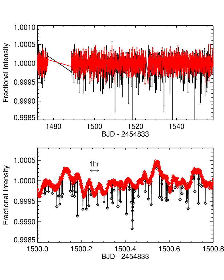
Figure 3.— Top panel: Full Quarter 16 short-cadence time series of HD 185351. Black and red data points show the time series before and after the outlier rejection procedure described in the text. Note that only 5% of all data is shown for clarity. Bottom panel: Same as the top panel but for a 1-day segment. Here, the data are shown with the original 1-minute sampling. Note the $\sim 1$ hour variability in the light curve which is due to oscillations in HD 185351.

Inspection of the raw data of HD 185351 showed a considerable number of outliers below the average flux level. We attribute these outliers to the increased pointing jitter during Q16, causing the photocenter to move sporadically outside the dedicated pixel mask. To reject these outliers we calculated the flux difference of each consecutive data point pair for the full time series. Then, all data points with a flux decrease greater than 3 times the standard deviation of the flux differences over the entire dataset were removed. This procedure was iterated until the residual scatter converged. Finally, we applied a Savitzky-Golay filter with a width of 2 days to the light curve to remove any instrumental and intrinsic low-frequency variability that could influence the oscillation signal, and applied a 4–$\sigma$ clipping using a 1-day moving mean. The detrended light curve with and without the adopted outlier rejection is shown in Figure 3.

2.4.3 Fundamental Properties from Scaling Relations

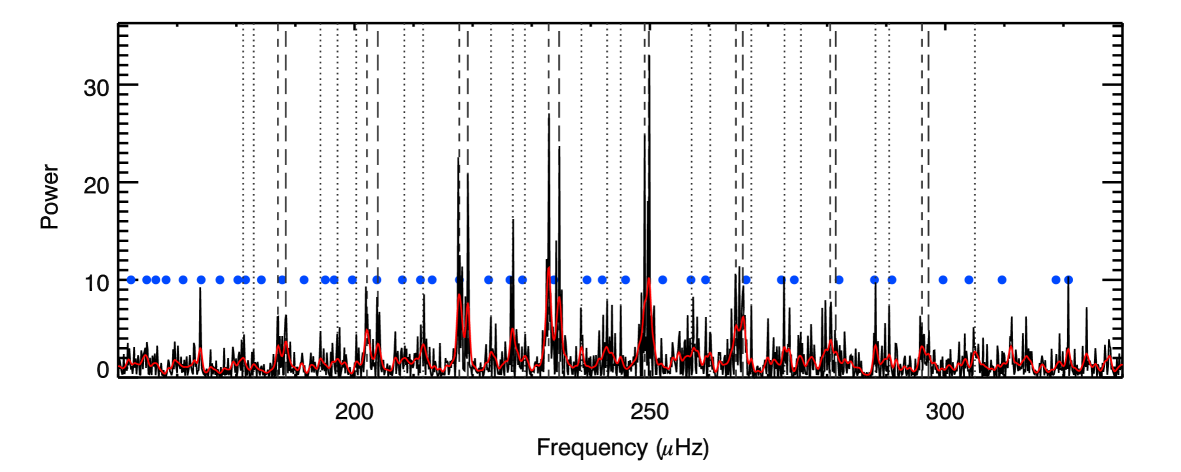
Figure 4.— Background-corrected power spectrum of HD 185351, with the smoothed power-spectrum shown in red. Long-dashed, dotted, and short-dashed lines indicate the locations of identified $l$=0, 1, and 2 modes, respectively. Expected locations of l=1 mixed modes from the asymptotic relation are indicated by blue circles.

We calculate the power spectrum from the detrended light curve using the method described by Huber et al. (2009) to model the background power due to stellar granulation and detect the signature of oscillations. Figure 4 shows the region of the background-corrected power spectrum centered on the detected power excess due to the stellar oscillations. The frequency of maximum power as measured from the smoothed, background–corrected power spectrum is $\nu_{\rm max}=229.8\pm 6.0~{}\mu$Hz. To measure the large frequency separation we calculated échelle diagrams with trial values of $\Delta\nu$ to align the $l=0$ modes, yielding $\Delta\nu=15.4\pm 0.2~{}\mu$Hz. The échelle diagram of HD 185351 is shown in Figure 5. Uncertainties on the measured values were estimated from Monte-Carlo simulations performed on synthetic power spectra calculated for a $\chi^{2}$ distribution with two degrees of freedom, as described in Huber et al. (2011). For each synthetic power spectrum the $\Delta\nu$ and $\nu_{\rm max}$ measurement was repeated, and the uncertainties were calculated as the standard deviation of the resulting distributions. We note that the $~{}1\%$ and $~{}3\%$ uncertainties on $\Delta\nu$ and $\nu_{\rm max}$ are compatible with typical uncertainties reported in the literature for Kepler observations (e.g., Hekker et al., 2011).

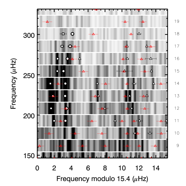
Figure 5.— Échelle diagram of HD 185351, showing fitted frequencies in white. Modes are identified as $l=0$ (circles), $l=1$ (triangles) and $l=2$ (squares). Expected l=1 mixed modes from the asymptotic relation are shown by the red open triangles, with horizontal bars showing the maximum expected rotational splitting. For reference, a grey-scale map of the smoothed power spectrum is shown in the background. Numbers to the right of the plot indicate radials order of the $l=0$ modes.

Our measured values of $\Delta\nu$ and $\nu_{\rm max}$ for HD 185351 are fully consistent with the relationships between both quantities (Stello et al., 2009b; Hekker et al., 2009; Mosser et al., 2010). Combining $\nu_{\rm max}$ and $\Delta\nu$ with the interferometric effective temperature derived in § 2.3 yields $R_{\star}$ $=5.35\pm 0.20$ $R_{\odot}$, $M_{\star}$ $=1.99\pm 0.23$ $M_{\odot}$, $\log{g}$ $=3.280\pm 0.014$ and $\rho_{\star}$ $=0.0130\pm 0.0003$ $\rho_{\odot}$. The adopted solar reference values, which were measured using the same method as applied to HD 185351, are $\nu_{\rm max,\sun}=3090~{}\mu$Hz, $\Delta\nu_{\sun}=135.1~{}\mu$Hz (Huber et al., 2011).

We note that modifications of the scaling relations suggested in the literature do not significantly change these results. Using stellar mass as an example, the corrections yield $M_{\star}$$=1.89$ $M_{\odot}$ using the relations by Mosser et al. (2013), and $M_{\star}$$=1.97~{}$$M_{\odot}$ using the relations by Wu et al. (2014). The $\Delta\nu$ correction by White et al. (2011) for stars with a temperature similar to HD 185351 is $<0.1\%$, and hence does not significantly change the stellar mass estimate.

In addition to evaluating Equations 2 and 3 directly, $\Delta\nu$ and $\nu_{\rm max}$ can be used as input values to interpolating evolutionary models. This method has the advantage of yielding smaller formal uncertainties since metallicity information can be taken into account, and unphysical solutions based on evolutionary theory are discarded (Gai et al., 2011). Combining $T_{\rm eff}$ and metallicity derived from the SME analysis with $\nu_{\rm max}$, $\Delta\nu$ and BaSTI evolutionary models (Pietrinferni et al., 2004) we derived an additional set of asteroseismic properties, yielding $R_{\star}$ $=5.27\pm 0.15$ $R_{\odot}$, $M_{\star}$ $=1.90\pm 0.15$ $M_{\odot}$, $\log{g}$ $=3.273\pm 0.014$ and $\rho_{\star}$ $=0.0130\pm 0.0003$ $\rho_{\odot}$. Our asteroseismic measurements of the stellar properties based on scaling relations are given in Table 1.

2.4.4 Mass Constraints from Mixed–Mode Period Spacings

In evolved stars, the dipole ($l=1$) mixed modes are particularly useful for determining stellar parameters and structure (e.g. Metcalfe et al., 2010; Bedding et al., 2011; Mosser et al., 2011; Beck et al., 2012; Benomar et al., 2012; Deheuvels et al., 2012). These modes occur when acoustic p-mode oscillations in the outer envelope of the star couple to g-mode (gravity) oscillations in the core (Osaki, 1975; Aizenman et al., 1977). The signature of mixed modes is clear in the échelle diagram in Figure 5, with several dipole modes in each radial order. While p modes of the same degree, $l$, and consecutive radial order, $n$, are approximately equally spaced in frequency, g modes are approximately equally spaced in period (Tassoul, 1980). Due to mode bumping, the observed period spacing of mixed modes will be significantly smaller than the true, underlying g–mode period spacing, $\Delta\Pi_{1}$. However, by measuring the observed period spacing, a lower limit may be placed on $\Delta\Pi_{1}$, and if a sufficient number of modes are observed, its value may be deduced.

According to models, evolved stars show a strong mass dependency on $\Delta\Pi_{1}$ (White et al., 2011; Stello et al., 2013). While this mass dependency is strongest during the subgiant phase (Benomar et al., 2012, 2013) the effect is still significant along the red giant branch for stars with non-degenerate or partially-degenerate cores, corresponding to $M\gtrsim 1.8~{}M_{\odot}$ (Stello et al., 2013). Hence, if HD 185351 does have a high mass, then the period spacing should reflect this.

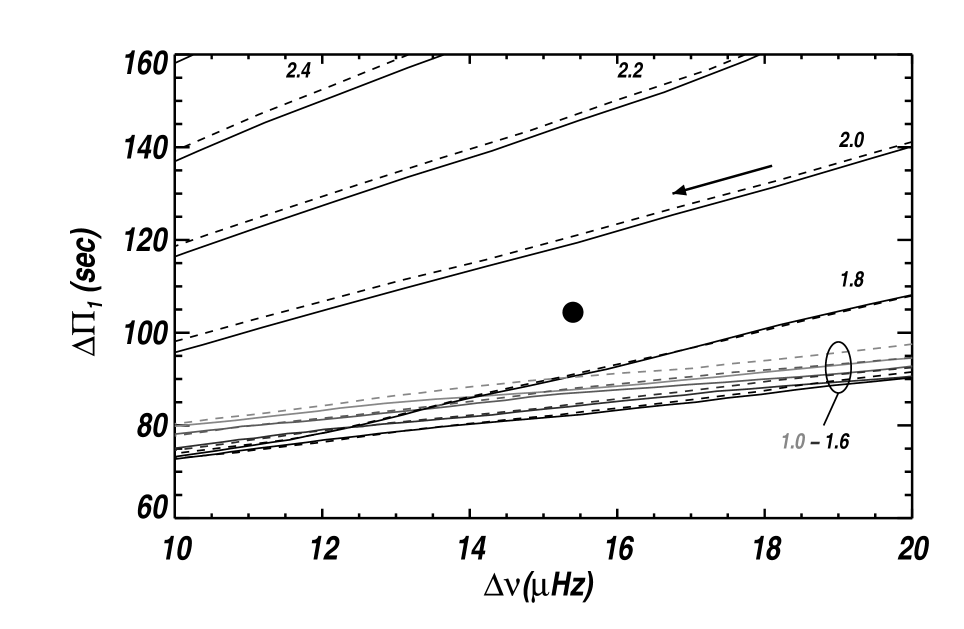
Figure 6.— Evolutionary model tracks showing the gravity mode period spacing for dipole modes, $\Delta\Pi_{1}$, as a function of the large frequency separation, $\Delta\nu$. The mass in solar units is indicated for each track. Solid lines are for models with Fe/H]=+0.0 dex, and dashed lines are for models with [Fe/H]=+0.2 dex. Lower mass tracks ($1.0<M/M_{\odot}<1.6$) are indicated by a black oval and are shown in greyscale with lower mass indicated by lighter grey. Stars evolve from right to left indicated by the arrow. The location of HD 185351 is shown by the black circle. The uncertainty in the measurements of $\Delta\Pi_{1}$ and $\Delta\nu$ is smaller than the symbol size.

To determine the value of $\Delta\Pi_{1}$ in HD 185351, we first measured the mode frequencies. The background-corrected power spectrum was smoothed by a Gaussian function with full-width at half maximum of $0.4~{}\mu$Hz, and significant peaks were identified. A global Markov chain Monte Carlo (MCMC) fit was made to the power spectrum with the frequencies, heights and widths of the identified modes as free parameters (e.g. Benomar et al., 2009; Handberg & Campante, 2011). The measured mode frequencies and their uncertainties are given in Table 4, and indicated in Figures 4 and 5. In many red giants observed by Kepler, $l=1$ modes are seen to be split by rotation into $m=0,\pm 1$ components (Beck et al., 2012; Deheuvels et al., 2012; Mosser et al., 2012b). However, no clear indication of this splitting can be found in HD 185351. This may be due to this power spectrum having a relatively low frequency resolution and signal-to-noise ratio compared to other Keplergiants. Alternatively, HD 185351 may have a low inclination, which suppresses the $m=\pm 1$ components (Gizon & Solanki, 2003).

We performed a MCMC fit of the asymptotic relation for mixed modes (Mosser et al., 2012a) to the observed $l=1$ modes to determine p– and g–mode parameters, assuming that only the $m=0$ component is present. The $l=0$ modes were included in the fit to constrain the p–mode parameters, such as $\Delta\nu$. We find the underlying g–mode period spacing $\Delta\Pi_{1}=104.7\pm 0.2~{}\mathrm{s}$. The locations of $l=1$ frequencies predicted from the asymptotic relation are indicated by the blue circles in Figure 4 and red triangles in Figure 5.

To investigate the possible impact of undetected rotational splitting on our measured period spacing, we determined the maximum expected rotational splittings following the results of Mosser et al. (2012b). Mixed modes that have a stronger $g$-mode character are more sensitive to the rotation rate in the core, while mixed modes that are dominated by a $p$-mode character are more sensitive to the envelope. The cores of red giants rotate substantially faster than their envelopes, and so the observed frequency splitting increases with $g$-mode characteristics. Mosser et al. (2012b) empirically described this variation in rotational splitting with a Lorentzian profile. For stars of a similar evolutionary state to HD 185351, they found the maximum rotational splitting in a star to vary between 0.2 and 0.6 $\mu$Hz. Taking 0.6 $\mu$Hz as a maximum expected rotational splitting for HD 185351, and the typical values Mosser et al. (2012b) found for the width and amplitude parameters of the Lorentzian profile, we calculated the rotational splittings for each of the asymptotic frequencies. The size of these splittings is shown by the horizontal bars on the red asymptotic frequencies in Figure 5. The spacing between the mixed modes is significantly larger than the expected rotational splittings, and so we conclude that the non-detection of rotational splittings has not impacted on our determination of the period spacing.

Figure 6 shows $\Delta\Pi_{1}$ for HD 185351 relative to a grid of models from Stello et al. (2013, solid) supplemented by a grid of super solar metallicity ([Fe/H] $+0.2$; dashed) that bracket the value of HD 185351. The models were generated using the MESA 1M_pre_ms_to_wd test suite (Paxton et al., 2011, 2013). MESA derives $\Delta\Pi_{1}$ from the integral of the buoyancy frequency and derives $\Delta\nu$ from the integral of the sound speed (see Stello et al., 2013; Paxton et al., 2013, for details). Stars evolve from right to left in this diagram caused by their expansion, and hence decrease in the mean density and $\Delta\nu$. Lower mass tracks ($M_{\star}<1.6~{}M_{\odot}$) show similar period spacings at a given $\Delta\nu$, while this degeneracy is lifted for more massive stars. We note that this analysis uses the metallicity measurement from SME, but $\Delta\Pi_{1}$ is minimally affected by metallicity as can be seen in Figure 6. By matching tracks through the position of HD 185351 in Figure 6 we find it to be consistent with a mass of 1.85–1.90 $M_{\odot}$. This mass range accounts for the fact that model values of $\Delta\nu$ are based on the integral of the sound speed, which shifts the tracks to the right by up to 3% relative to the observed value (Stello et al., 2009b).

While the mass estimate based on mixed modes is model-dependent, the period spacing probes the conditions in the stellar core and hence provides valuable independent information compared to other model-dependent mass estimates based on atmospheric properties. More detailed modelling of the oscillations, which has been done for other stars (e.g. Metcalfe et al., 2010; Di Mauro et al., 2011) but is beyond the scope of this paper, may provide a precise measurement of the age of HD 185351.

3. Results

The results of our various independent analyses, and the constraints they place on the mass of HD 185351 are summarized in Figure 7. This concordance diagram plots effective temperature versus surface gravity ($\log{g}$), at a fixed [Fe/H]$=+0.16$. The small dots are discrete points sampled from the BaSTI stellar evolution models, which are better sampled and thus better visualized along the subgiant and giant regions of the H–R diagram than are the Y2 models used in § 2.1. The colored bands illustrate the constraints provided by our interferometric, astrometric and spectroscopic analyses, with widths showing the 1–$\sigma$ confidence regions. For example, our $T_{\rm eff}$ estimates from SME and our SED fit are shown as vertical magenta and cyan bands, respectively, and have significant overlap, lending confidence that we have derived the temperature of HD 185351 both accurately and precisely.

Our asteroseismic constraints are shown as red and green, roughly horizontal bands, based on the large separation ($\Delta\nu$) and the frequency of maximum oscillation power ($\nu_{\rm max}$). These bands cross at roughly $T_{\rm eff}$ $=5050$ K, in the region of overlap from the independent measurements of $T_{\rm eff}$, corresponding to $M_{\star}$ $\approx 2$ $M_{\odot}$.

The final constraint illustrated on this figure is provided by the interferometric measurement of the stellar radius, $R_{\star}$ $=4.97\pm 0.07$ $R_{\odot}$ (blue). Iso-radius contours in the $\log{g}$–$T_{\rm eff}$ plane run roughly from lower left to upper right in this diagram. As evident by the position of the blue band with respect to the other constraints, there is some tension at the $2$–$3\sigma$ level between the mass constraint provided by the radius estimate and the asteroseismic and spectroscopic measurements. However, in the region where most of our constraints overlap, near $T_{\rm eff}$ $4980$ K, corresponds to $\sim 1.7$ $M_{\odot}$. Thus, all of our independent measurements of the mass of HD 185351 are consistent with masses $M_{\star}$ $>1.5$ $M_{\odot}$.

It should be noted that Figure 7 illustrates our mass constraints with respect to a theoretical model grid. One of the primary motivations of our study is to test the accuracy of these types of stellar evolution models using independent measurements. Table 1 lists our estimates of various stellar parameters using different combinations of our measurements. Column 1 lists the full set of stellar parameters, spectroscopic and physical, that we obtain from a combination of our SME spectral analysis and the interpolation of these spectroscopic parameters onto the Y2 stellar evolution model grids. This is the standard technique used to estimate the masses of isolated field stars, as in, e.g., Valenti & Fischer (2005); Takeda et al. (2007); Hekker & Meléndez (2007); Takeda et al. (2008); Johnson et al. (2007, 2013). These are the parameters that we wish to test with our various methods. In the following subsections we describe the outcome of these comparisons for individual stellar parameters.

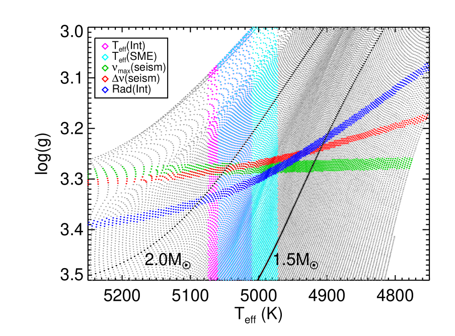
Figure 7.— Surface gravity versus temperature for the BaSTI evolutionary tracks (Pietrinferni et al., 2004) with [Fe/H]$=+0.16$ (Pietrinferni et al., 2004), as measured from our LTE spectral analysis. Colored models show the 1–$\sigma$ constraints from our observations: effective temperature derived from the interferometric angular diameter and bolometric flux (magenta), effective temperature from spectroscopy (cyan), $M_{\star}$$R_{\star}$^-2 $T_{\rm eff}$^-0.5 from the frequency of maximum power (green), density derived from the large frequency separation (red), and radius from the interferometric angular diameter and Hipparcos parallax (blue). Black lines highlight masses of 1.5 $M_{\odot}$ and 2.0 $M_{\odot}$, respectively.

3.1. Effective Temperature

The effective temperature of HD 185351 is determined using two approaches. One method, presented in § 2.3, makes use of the Stefan-–Boltzmann law, together with our measurements of the parallax-based distance, stellar angular diameter ($\theta$) and bolometric flux ($F_{\rm bol}$), which gives $T_{\rm eff}$ $=5042\pm 32$ K. We consider this method to be empirical in that it relies only weakly model-based assumptions (e.g. limb-darkening), and it sidesteps the intricacies and assumptions employed in modeling the observed stellar spectrum, which often relies on the assumption of plane-parallel atmospheres in LTE, among other simplifications. The star’s spectral energy distribution is used to estimate the bolometric flux, but we do so using observed stellar spectra of stars with well-measured $F_{\rm bol}$, rather than relying on synthetic spectra. However, checking our result based on empirical spectra against model spectra shows close agreement (§ 2.3).

We find very close agreement between our SED-based measurement of the effective temperature, and that of our SME analysis. This bolsters the reliability of previous estimates of giant and subgiant stellar properties using LTE spectral modeling since systematic errors in $T_{\rm eff}$ can lead to large errors in $M_{\star}$ and $R_{\star}$ (e.g. Valenti & Fischer, 2005; Lloyd, 2013).

3.2. Surface Gravity

Our LTE spectral synthesis modeling is implemented using SME, which models the stellar surface gravity by fitting to the damping wings of the Mg II b triplet lines (Valenti & Piskunov, 1996; Valenti & Fischer, 2005). This method works well for $\log{g}$ $\gtrsim 4$, but the uncertainty increases for lower surface gravity due to significant weakening of the Mg II b damping wings. Also, $\log{g}$ is correlated with both $T_{\rm eff}$ and [Fe/H] in SME, which can bias the model-grid-interpolated stellar mass (Torres et al., 2012; Huber et al., 2013). It is therefore worthwhile to compare our asteroseismic and spectroscopic values of $\log{g}$.

As seen in Table 1, our SME analysis yields $\log{g}$ $=3.31\pm 0.06$, which compares well with the value obtained from $\nu_{\rm max}$ ($\log{g}$ $=3.280\pm 0.011$). Equation 3 shows that the effective temperature enters into the asteroseismic estimate of $\log{g}$, but it does so only weakly as $T_{\rm eff}$^-1/2, and as a result, errors on $T_{\rm eff}$ propagate weakly, as $\frac{1}{2}\sigma_{T_{\rm eff}}^{2}$. The fractional uncertainty on our SED-based $T_{\rm eff}$ is $\sim 1$%, and are therefore negligible compared to the measurement errors in our asteroseismic values of $\nu_{\rm max}$ and $R_{\star}$, which are 2.6% and 3.8%, respectively.

Just as with our estimates of $T_{\rm eff}$, we find close agreement between our empirical measurement and model-based estimate of $\log{g}$, which is remarkable given the low surface gravity of HD 185351. This is likely a result of the iterative scheme used in our SME analysis, which differs from the unconstrained SME analysis employed in the critical evaluation of SME in Torres et al. (2012).

3.3. Mean Density

Our model-grid interpolation of our spectroscopic parameters from SME provide an estimate of the mean stellar density, giving $\rho_{\star}$ $=0.014\pm 0.004$ g cm^-3. We also estimate $\rho_{\star}$ using the large frequency separation observed in our asteroseismic measurements, $\Delta\nu$, which gives $\rho_{\star}$ $=0.0130\pm 0.0003$ g cm^-1/3. We therefore find close agreement between our model-based and empirical estimates of another key physical characteristic of HD 185351.

3.4. Radius

The interpolation of our SME parameters onto stellar evolution model grids also provides an estimate of the stellar radius, giving $R_{\star}$ $=5.07\pm 0.16$ $R_{\odot}$. Our interferometric measurements compare well with this value, yielding $R_{\star}$ $=4.97\pm 0.07$ $R_{\odot}$, resulting in a 0.6–$\sigma$ agreement (relative to the quadrature-sum of the two errors) between our model-based and empirical measurement.

We also estimate $R_{\star}$ using our asteroseismic measurements of $\Delta\nu$ and $\nu_{\rm max}$, combined with our $T_{\rm eff}$ measurement from interferometry, which gives $R_{\star}$ $=5.35\pm 0.20$ $R_{\odot}$. This agrees with our model–based estimate to within 1–$\sigma$. Our interferometric and asteroseismic values of $R_{\star}$ bracket our SME$+$model grid value, and the weighted average of our two empirical measurements is $R_{\star}$ $=4.98\pm 0.01$ $R_{\odot}$, which agrees with the model-based value to 0.56 $\sigma$.

As described in § 2.4, we also measured the stellar radius using our asteroseismic measurements under the constraints provided by our SME-based metallicity ([Fe/H]) and the BaSTI stellar evolution models. This gives $R_{\star}$ $=5.27\pm 0.15$ $R_{\odot}$, which is larger than, but comparable within errors to all of our other measurements.

3.5. Mass

The key physical parameter of interest for evolved stars like HD 185351 is stellar mass. Our model-based estimate, measured using spectral synthesis and model-grid interpolation, is $M_{\star}$ $=1.87\pm 0.07$ $M_{\odot}$. This value agrees well with our asteroseismic-only measurement made by combining Equations 2 and 3 ($M_{\star}$ $=1.99\pm 0.23$ $M_{\odot}$). We also find close agreement with the mass measured by interpolating the asteroseismic $\log{g}$ and $\rho_{\star}$, plus the spectroscopic [Fe/H] and $T_{\rm eff}$, onto the BaSTI model grids ($M_{\star}$ $=1.90\pm 0.15$ $M_{\odot}$). This second model-based procedure is illustrated in Figure 7 in the region of overlap among the asteroseismic parameters and SED $T_{\rm eff}$.

We also estimated the stellar mass by combining the asteroseismic density calculated from the large frequency spacing $\Delta\nu$ (cf Equation 2) with the interferometric radius. This is our least model-dependent estimate of the stellar mass in that it is independent of any aspect of our SME spectral analysis and evolution models, which are under scrutiny in this study. We find $M_{\star}$ $=1.60\pm 0.08$$M_{\odot}$, which is smaller than our SME model-based value by 2.6 $\sigma$. The value is also smaller than the mass derived from asteroseismic scaling relations (by 1.6 $\sigma$), asteroseismic scaling relations combined with BaSTI models (by 1.8 $\sigma$), and the mass implied from the gravity mode period spacing.

As illustrated in our concordance diagram (Figure 7), the mass difference could be reconciled either by a systematic increase in the interferometric radius (upward shift of blue band) or a systematic increase in $\Delta\nu$ and $\nu_{\rm max}$ (downward shift of red and green bands). The required offsets in measured quantities are a $\sim$5% decrease in the parallax, a $\sim$6% increase in angular diameter, or a 9% increase in $\Delta\nu$ and $\nu_{\rm max}$. HD 185351 is a photometric standard star with no indication of a binary companion, and hence a systematic error in the Hipparcos parallax is unlikely. While angular diameters can be affected by systematic calibration errors, the agreement of our estimates using two different instruments and different calibrators rule out a shift as a large as 6%. Corrections to asteroseismic scaling relations for stars that are more evolved than the Sun have been proposed, but so far theoretical investigations and empirical tests have ruled out offsets as large as 9% for $\Delta\nu$ and $\nu_{\rm max}$. In summary, the tension between the our lowest mass measurement and other estimates is likely not due to a systematic error in one of the adopted methods, but could be due to a combined effect of small offsets in the different measurements.

Another possible explanation for the disagreement stems from the different methods we used to measure the stellar radius. Interferometry, together with the parallax–based distance, provides a measure of the Rosseland, or mean emitting surface of the star, which roughly corresponds to the point at which the optical depth $\tau=2/3$. The radius measured from asteroseismology corresponds to the radial location where pressure waves are reflected back into the stellar interior. This occurs where the frequency of the pressure wave is smaller than the acoustic cut-off frequency, $\nu_{\rm ac}$, which for isothermal conditions depends on the sound speed and the pressure scale height (see § 2.4.1). If the point in the stellar interior where $\nu_{\rm max}\approx\nu_{\rm ac}$ differs from the location of the $\tau=2/3$ surface, then our two methods of measuring the stellar radius will differ.

To investigate this possibility, we examined the interior structure of a MESA model of a giant star similar to HD 185351, specifically the acoustic cutoff frequency and mean emitting surface in the outer 1% of its radius. We find that the $\nu_{\rm max}\approx\nu_{\rm ac}$ surface is slightly below the $\tau=2/3$ surface. However, the difference is only 0.1%, well below our measurement uncertainties. While this result is model–dependent, it is unlikely that the true difference is more than an order of magnitude larger than this, which is the amount required to explain the discrepancy between our various radius, and hence mass, measurements.

4. Summary and Discussion

Our knowledge of the masses and radii of the vast majority of stars in the Galaxy rests on our theoretical understanding of stellar atmospheres and stellar evolution. For example, the process of measuring the mass of an isolated star typically begins with a measure of its effective temperature and metallicity from its observed spectrum, and its parallax-based luminosity (e.g. Johnson et al., 2013). For stars lacking a precise distance estimate, a spectroscopically-measured surface gravity ($\log{g}$), or its stellar density ($\rho_{\star}$), can serve as a proxy for luminosity (e.g. Seager & Mallén-Ornelas, 2003; Sozzetti et al., 2007). These properties define the star’s location within the theoretical Herzsprung–Russell diagram, which in turn depends on the star’s evolutionary state as dictated by its mass, chemical composition and age. Theoretical H–R diagrams have been computed by many groups by integrating the equations of stellar structure forward in time with various initial stellar masses and chemical compositions, and the results are tabulated in what are commonly referred to as stellar evolution model grids (e.g. Demarque et al., 2004). Thus, a star’s mass can be estimated by interpolating its observed properties onto these grids and recording the corresponding stellar mass, as well as other physical properties such as radius, mean density, internal structure (e.g. core helium fraction) and age (e.g. Valenti & Fischer, 2005; Hekker & Meléndez, 2007; Takeda et al., 2008; Do Nascimento et al., 2010).

Models of stellar atmospheres and evolution are most reliable for stars similar to the Sun, which is by far the best characterized star in the Galaxy. For locations in the H–R diagram that lie far from the Sun’s position or for stars with different chemical compositions, theoretical atmosphere and evolution models are less robust. In these regions it is important to gather independent measurements of stellar physical characteristics that can be used to critically examine model predictions and provide touchstones for studies of stars of similar types.

Our study focuses on an evolved star, HD 185351  which is one of several giant stars targeted by the Doppler-based planet survey of Johnson et al. (2011). Stars such as HD 185351 may be proxies of more massive main-sequence stars that are not amenable to precision Doppler-shift measurements owing to their rotationally-broadened absorption features. After evolving off of the main sequence, massive, hot stars shed most of their angular momentum and cool down, making them better targets for Doppler surveys. Johnson et al. (2007) and Johnson et al. (2010) have reported an apparent increase in the occurrence rate of giant planets around evolved stars more massive than the Sun. This has been interpreted as support for the core accretion theory of planet formation since the disks around more massive stars presumably contain more mass, and hence more of the building blocks for the protoplanetary cores that eventually become gas giants. However, the masses of these evolved stars have been called into question, raising concerns that giant stars like HD 185351, which have model-grid-based masses in excess of 1.5 $M_{\odot}$, may in fact have masses comparable to Sun-like dwarfs (Lloyd, 2013; Schlaufman & Winn, 2013). If this were the case, then the apparent enhanced planet occurrence rate observed around subgiant and giant stars discovered by would require critical reexamination and perhaps a different interpretation.

There are two likely sources of systematic errors in estimating the masses of giant stars like HD 185351. The first is in the measurement of atmospheric parameters ($T_{\rm eff}$, $\log{g}$, [Fe/H]) by fitting LTE spectral models to observed spectra, which in our case is performed using the widely-used SME software package (Valenti & Fischer, 2005). If the effective temperature measured using this technique were off by, e.g., 200 K then the inferred stellar mass from evolutionary models would be in error by as much as 0.3 $M_{\odot}$, or 20% at the base of the red giant branch. A similar systematic error in the stellar mass would result from a 0.2 dex inaccuracy in $\log{g}$.

Our study suggests that systematic errors in the effective temperature and surface gravity measured using SME are much smaller than 200 K and 0.2 dex, respectively. Indeed, our temperature measured from a combination of the interferometric stellar radius and bolometric luminosity agrees to well within errors with the temperature from SME. Similarly, the SME-based surface gravity agrees within errors with the asteroseismic $\log{g}$ estimated from the observed frequency of maximum oscillation power.

The second potential source of error in measuring the mass of giant stars is in the interpolation of the atmospheric properties onto stellar evolution model grids. Improper treatment of core overshoot, the convective mixing length parameter or other subtleties in the evolution of giant stars may lead to an inaccurate mapping of stellar physical characteristics such as mass and radius to observed properties such as luminosity, metallicity and effective temperature. We tested the veracity of the model grids by comparing the model-grid interpolated mass and radius of HD 185351 to the mass and radius measured from asteroseismology and interferometry, respectively.

Interpolating the spectroscopic parameters of HD 185351 onto the Yonsei-Yale model grids results in a mass of $1.87\pm 0.07$ $M_{\odot}$. The observed large frequency spacing and frequency of maximum oscillation observed in our Kepler photometry yield a mass that agrees well with this estimate, giving $1.99\pm 0.23$ $M_{\odot}$. While stellar evolution models require assumptions about the complicated interplay of the interior structure of stars and the radiative transfer processes occurring in the stellar photosphere, asteroseismology provides direct measures of the bulk properties of the star, namely the mean density and surface gravity, which in turn are related to the stellar mass and radius. Thus, the agreement between our asteroseismic mass and radius and that predicted by a combination of atmospheric parameters and stellar evolution models indicates that the models are not plagued by large systematic errors.

Our observation of mixed p– and g–modes in the oscillation spectrum of HD 185351 provides another asteroseismic mass estimate. The period spacing of the mixed modes, $\Delta\Pi_{1}$, can be compared to the predictions of interior structure models (cf § 2.4.4). As shown in Figure 6, our observed period spacing is consistent with the mass measured from evolution model grids and asteroseismic scaling relations. These predictions, while based on interior structure models, are independent from the scaling relations used to relate the other asteroseismic parameters to stellar mass and radius. Thus, we have two independent measures of the stellar mass that agree with the mass found from model grid interpolation.

We find some tension, at the 2.6–$\sigma$ level, to our least model-dependent mass measurement based on a combination of our interferometric radius and the density from asteroseismology. This disagreement stems primarily from a smaller radius measured from interferometry compared to the radius measured from asteroseismology. It may be that our other independent mass measurements contain independent systematic errors that result in a mass that is incorrect. Alternatively, the difference could be due to a combination of small biases in the $\Delta\nu$ scaling relation used to derive the mean stellar density and the measured angular diameter. Additionally, there may also exist systematic errors at the $\sim 5$% level in the model grids which contribute to this difference. It is possible that our sample of one just happens to have an interferometric mass estimate that is low due to statistical errors.

The disagreement between some of our independent mass estimates motivates further investigation using the observational techniques described herein. We are currently gathering additional asteroseismic and interferometric observations of bright, nearby evolved stars to perform a more in-depth statistical analysis of various model grids in the subgiant/giant region of the H–R diagram. However, even after adopting our smallest stellar mass estimate, we conclude that HD 185351 has a mass that is significantly higher than that of the Sun and consistent with that an early F– or A–type dwarf star.

Table 1

Stellar	LTE Spectroscopic Fit	Asteroseismology	Interferometry	Asteroseismology	Interferometry
Parameter	$+$ Evolution Model	Only	and SED Fitting	$+$ Spectroscopy	$+$Asteroseismology
				$+$Evolution Model
R⋆ ($R_{\odot}$)	5.07 $\pm$ 0.16	5.35 $\pm$ 0.20	4.97 $\pm$ 0.07	5.27 $\pm$ 0.15	…
$\rho_{\star}$ ($\rho_{\odot}$)	0.014 $\pm$ 0.004	0.0130 $\pm$ 0.0003	…	0.0130 $\pm$ 0.0003	…
$\log{g}$ (cgs)	3.31 $\pm$ 0.06	3.280 $\pm$ 0.011	…	3.273 $\pm$ 0.014	…
$T_{\rm eff}$ (K)	5016 $\pm$ 44	…	5042 $\pm$ 32	…	…
$[{\rm Fe/H}]$	+0.16 $\pm$ 0.04	…	…	…	…
M⋆ ($M_{\odot}$)	1.87  $\pm$ 0.07	1.99  $\pm$ 0.23	…	1.90  $\pm$ 0.15	1.60  $\pm$ 0.08

Table 2Log of interferometric observations.

UT Date	Combiner	Baseline	No. of scans	Calibrators
2012 August 6	Classic	S2-W1	8	HD 186176, HD 188667
2012 August 7	Classic	S2-W1	5	HD 186176, HD 188667
2012 August 11	PAVO	W1-W2	2	HD 188665
2013 July 7	PAVO	W1-W2	5	HD 177003, HD 185872, HD 188252
2014 April 6	PAVO	W1-W2	1	HD 185872
2014 April 7	PAVO	W1-W2	2	HD 177003, HD 185872
2014 April 10	PAVO	E2-W2	1	HD 184784, HD 188252

Table 3Measured Angular Diameters.

Combiner	$\mu_{\lambda}$	$\theta_{\mathrm{UD}}$	$\theta_{\mathrm{LD}}$	$R$
		(mas)	(mas)	($R_{\odot}$)
Classic	0.32$\pm$0.04	1.089$\pm$0.016	1.120$\pm$0.018	4.92$\pm$0.09
PAVO	0.64$\pm$0.03	1.064$\pm$0.009	1.133$\pm$0.013	4.97$\pm$0.07
Classic + PAVO	…	…	1.132$\pm$0.012	4.97$\pm$0.07

Table 4Measured frequencies of HD 185351.

n	l=0	l=1	l=2
	($\mu$Hz)	($\mu$Hz)	($\mu$Hz)
10	…	181.16$\pm$0.21	187.05$\pm$0.09
		182.94$\pm$0.26
11	188.38$\pm$0.10	194.24$\pm$0.09	202.11$\pm$0.14
		197.12$\pm$0.35
		200.31$\pm$0.07
12	203.95$\pm$0.18	208.45$\pm$0.38	217.74$\pm$0.12
		211.62$\pm$0.23
13	219.19$\pm$0.08	223.10$\pm$0.12	232.86$\pm$0.11
		226.80$\pm$0.14
		228.85$\pm$0.14
14	234.64$\pm$0.13	238.41$\pm$0.12	249.11$\pm$0.19
		242.76$\pm$0.25
		245.06$\pm$0.05
15	249.83$\pm$0.17	257.06$\pm$0.91	264.56$\pm$0.17
		260.21$\pm$0.11
16	265.73$\pm$0.16	267.17$\pm$0.06	280.51$\pm$0.23
		272.79$\pm$0.18
		275.57$\pm$0.65
17	281.46$\pm$0.29	288.19$\pm$0.08	296.06$\pm$0.36
		290.51$\pm$0.07
18	297.16$\pm$0.19	305.02$\pm$0.24	…

References

- Aizenman et al. (1977) Aizenman, M., Smeyers, P., & Weigert, A. 1977, A&A, 58, 41
- Allende Prieto & Lambert (1999) Allende Prieto, C., & Lambert, D. L. 1999, A&A, 352, 555
- Argue (1963) Argue, A. N. 1963, MNRAS, 125, 557
- Argue (1966) Argue, A. N. 1966, MNRAS, 133, 475
- Baines et al. (2011) Baines, E. K., McAlister, H. A., ten Brummelaar, T. A., et al. 2011, ApJ, 743, 130
- Basri et al. (2005) Basri, G., Borucki, W. J., & Koch, D. 2005, New Astron. Rev., 49, 478
- Bazot et al. (2011) Bazot, M., Ireland, M. J., Huber, D., et al. 2011, A&A, 526, L4
- Beck et al. (2012) Beck, P. G., Montalbán, J., Kallinger, T., et al. 2012, Nature, 481, 55
- Bedding et al. (2011) Bedding, T. R., Mosser, B., Huber, D., et al. 2011, Nature, 471, 608
- Beichman et al. (1988) Beichman, C. A., Neugebauer, G., Habing, H. J., Clegg, P. E., & Chester, T. J. 1988, Infrared astronomical satellite (IRAS) catalogs and atlases. Volume 1: Explanatory supplement, 1
- Belkacem et al. (2011) Belkacem, K., Goupil, M. J., Dupret M. A., et al. 2011, A&A, 530, A142
- Belkacem (2012) Belkacem, K. 2012, SF2A-2012: Proceedings of the Annual meeting of the French Society of Astronomy and Astrophysics, 173
- Brogaard et al. (2012) Brogaard, K., VandenBerg, D. A., Bruntt, H., et al. 2012, A&A, 543, 106
- Benomar et al. (2009) Benomar, O., Baudin, F., Campante T. L., et al. 2009, A&A, 507, L13
- Benomar et al. (2012) Benomar, O., Bedding, T. R., Stello, D., et al. 2012, ApJ, 745, L33
- Benomar et al. (2013) Benomar, O., Bedding, T. R., Mosser, B., et al. 2013, ApJ, 767, 158
- Bildsten et al. (2012) Bildsten, L., Paxton, B., Moore, K., & Macias, P. J. 2012, ApJ, 744, L6
- Bohlin & Gilliland (2004) Bohlin, R. C. & Gilliland, R. L. 2004 AJ127, 3508
- Bonneau et al. (2006) Bonneau, D., Clausse, J.-M., Delfosse, X., et al. 2006, A&A, 456, 789
- Bonneau et al. (2011) Bonneau, D., Delfosse, X., Mourard, D., et al. 2011, A&A, 535, A53
- Bowler et al. (2010) Bowler, B. P., Johnson, J. A., Marcy, G. W., et al. 2010, ApJ, 709, 396
- Boyajian et al. (2012a) Boyajian, T. S., McAlister, H. A., van Belle, G., et al. 2012, ApJ, 746, 101
- Boyajian et al. (2012b) Boyajian, T. S., von Braun, K., van Belle, G., et al. 2012, ApJ, 757, 112
- Boyajian et al. (2013) Boyajian, T. S., von Braun, K., van Belle, G., et al. 2013, ApJ, 771, 40
- Brown et al. (1991) Brown, T. M., Gilliland, R. L., Noyes, R. W., et al. 1991, ApJ, 368, 559
- Brown et al. (2011) Brown, T. M., Latham, D. W., Everett, M. E., & Esquerdo, G. A. 2011, AJ, 142, 112
- Burnashev (1985) Burnashev, B. I. 1985, Bulletin Crimean Astrophysical Observatory, 66, 152
- Castelli & Kurucz (2004) Castelli, F., & Kurucz, R. L. 2004, arXiv:astro-ph/0405087
- Claret & Bloemen (2011) Claret, A., & Bloemen, S. 2011, A&A, 529, A75
- Crepp & Johnson (2011) Crepp, J. R., & Johnson, J. A. 2011, ApJ, 733, 126
- Cutri et al. (2003) Cutri, R. M., Skrutskie, M. F., van Dyk, S., et al. 2003, ”The IRSA 2MASS All-Sky Point Source Catalog, NASA/IPAC Infrared Science Archive.
- Demarque et al. (2004) Demarque, P., Woo, J.-H., Kim, Y.-C., & Yi, S. K. 2004, ApJS, 155, 667
- Derekas et al. (2011) Derekas, A., Kiss, L. L., Borkovits, T., et al. 2011, Science, 332, 216
- Deheuvels et al. (2012) Deheuvels, S., García, R. A., Chaplin, W. J., et al. 2012, ApJ, 756, 19
- Di Mauro et al. (2011) Di Mauro, M. P., Cardini, D., Catanzaro G., et al. 2011, MNRAS, 415, 3783
- do Nascimento et al. (2000) do Nascimento, J. D., Jr., Charbonnel, C., Lèbre, A., de Laverny, P., & De Medeiros, J. R. 2000, A&A, 357, 931
- Do Nascimento et al. (2010) Do Nascimento, J. D., da Costa, J. S., & de Medeiros, J. R. 2010, A&A, 519, A101
- Eggen (1968) Eggen, O. J. 1968, London, H.M.S.O., 1968.
- Eggleton et al. (1973) Eggleton, P. P., Faulkner, J., & Flannery, B. P. 1973, A&A, 23, 325
- Frandsen et al. (2013) Frandsen, S., Lehmann, H., Hekker, S., et al. 2013, A&A, 556, A138
- Frink et al. (2002) Frink, S., Mitchell, D. S., Quirrenbach, A., et al. 2002, ApJ, 576, 478
- Galland et al. (2005) Galland, F., Lagrange, A.-M., Udry, S., et al. 2005, A&A, 443, 337
- Gai et al. (2011) Gai, N., Basu, S., Chaplin, W. J., et al. 2011, ApJ, 730, 63
- Gizon & Solanki (2003) Gizon, L., & Solanki, S. K. 2003, ApJ, 589, 1009.
- Glushneva et al. (1983) Glushneva, I. N., Doroshenko, V. T., Fetisova, T. S., et al. 1983, Trudy Gosudarstvennogo Astronomicheskogo Instituta, 53, 50
- Golay (1972) Golay, M. 1972, Vistas in Astronomy, 14, 13
- Gray & Nagar (1985) Gray, D. F., & Nagar, P. 1985, ApJ, 298, 756
- Häggkvist & Oja (1966) Häggkvist, L., & Oja, T. 1966, Arkiv for Astronomi, 4, 137
- Haggkvist & Oja (1987) Haggkvist, L., & Oja, T. 1987, A&AS, 68, 259
- Hanbury Brown et al. (1974) Hanbury Brown, R., Davis, J., Lake, R. J. W., & Thompson, R. J. 1974, MNRAS, 167, 475
- Handberg & Campante (2011) Handberg, R., & Campante T. L. 2011, A&A, 527, A56
- Hatzes et al. (2003) Hatzes, A. P., Cochran, W. D., Endl, M., et al. 2003, ApJ, 599, 1383
- Hatzes et al. (2012) Hatzes, A. P., Zechmeister, M., Matthews, J., et al. 2012, A&A, 543, A98
- Hekker & Meléndez (2007) Hekker, S., & Meléndez, J. 2007, A&A, 475, 1003
- Hekker et al. (2009) Hekker, S., Kallinger, T., Baudin, F., et al. 2009, A&A, 506, 465
- Hekker et al. (2010) Hekker, S., Debosscher, J., Huber, D., et al. 2010, ApJ, 713, L187
- Hekker et al. (2011) Hekker, S., Elsworth, Y., De Ridder, J., et al. 2011, A&A, 525, A131
- Howarth (2011) Howarth, I. D. 2011, MNRAS, 413, 1515
- Huber et al. (2009) Huber, D., Stello, D., Bedding, T. R., et al. 2009, CoAst, 160, 74
- Huber et al. (2011) Huber, D., Bedding, T. R., Stello, D., et al. 2011, ApJ, 743, 143
- Huber et al. (2012) Huber, D., Ireland, M. J., Bedding, T. R., et al. 2012, ApJ, 760, 32
- Huber et al. (2013) Huber, D., Chaplin, W. J., Christensen-Dalsgaard, J., et al. 2013, ApJ, 767, 127
- Huber et al. (2013) Huber, D., Carter, J. A., Barbieri, M., et al. 2013, Science, 342, 331
- Huber (2014) Huber, D. 2014, ArXiv e-prints (arxiv:1404.7501)
- Ireland et al. (2008) Ireland, M. J., Mérand, A., ten Brummelaar, T. A., et al. 2008, Proc. SPIE, 7013,
- Kornilov et al. (1991) Kornilov, V. G., Volkov, I. M., Zakharov, A. I., et al. 1991, Trudy Gosudarstvennogo Astronomicheskogo Instituta, 63, 4
- Mermilliod (1986) Mermilliod, J.-C. 1986, Catalogue of Eggen’s UBV data., 0 (1986), 0
- McClure & Forrester (1981) McClure, R. D., & Forrester, W. T. 1981, Publications of the Dominion Astrophysical Observatory Victoria, 15, 439
- Jennens & Helfer (1975) Jennens, P. A., & Helfer, H. L. 1975, MNRAS, 172, 667
- Jiang et al. (2011) Jiang, C., Jiang, B. W., Christensen-Dalsgaard, J., et al. 2011, ApJ, 742, 120
- Johnson et al. (2006) Johnson, J. A., Marcy, G. W., Fischer, D. A., et al. 2006, ApJ, 647, 600
- Johnson et al. (2006) Johnson, J. A., Marcy, G. W., Fischer, D. A., et al. 2006, ApJ, 652, 1724
- Johnson et al. (2007) Johnson, J. A., Fischer, D. A., Marcy, G. W., et al. 2007, ApJ, 665, 785
- Johnson et al. (2007) Johnson, J. A., Butler, R. P., Marcy, G. W., et al. 2007, ApJ, 670, 833
- Johnson et al. (2010) Johnson, J. A., Howard, A. W., Bowler, B. P., et al. 2010, PASP, 122, 701
- Johnson et al. (2010) Johnson, J. A., Aller, K. M., Howard, A. W., & Crepp, J. R. 2010, PASP, 122, 905
- Johnson et al. (2011) Johnson, J. A., Clanton, C., Howard, A. W., et al. 2011, ApJS, 197, 26
- Johnson et al. (2013) Johnson, J. A., Morton, T. D., & Wright, J. T. 2013, ApJ, 763, 53
- Kennedy & Kenyon (2008) Kennedy, G. M., & Kenyon, S. J. 2008, ApJ, 673, 502
- Keenan & McNeil (1989) Keenan, P. C., & McNeil, R. C. 1989, ApJS, 71, 245
- Kjeldsen & Bedding (1995) Kjeldsen, H. & Bedding, T. R. 1995, A&A, 293, 87
- Koch et al. (2010) Koch, D. G., Borucki, W. J., Basri, G., et al. 2010, ApJ, 713, L79
- Laughlin et al. (2004) Laughlin, G., Bodenheimer, P., & Adams, F. C. 2004, ApJ, 612, L73
- Lagrange et al. (2010) Lagrange, A.-M., Bonnefoy, M., Chauvin, G., et al. 2010, Science, 329, 57
- Lloyd (2011) Lloyd, J. P. 2011, ApJ, 739, L49
- Lloyd (2013) Lloyd, J. P. 2013, ApJ, 774, L2
- Lovis & Mayor (2007) Lovis, C., & Mayor, M. 2007, A&A, 472, 657
- Maestro et al. (2013) Maestro, V., Che, X., Huber, D., et al. 2013, MNRAS, 434, 1321
- Marois et al. (2008) Marois, C., Macintosh, B., Barman, T., et al. 2008, Science, 322, 1348
- Metcalfe et al. (2010) Metcalfe, T. S., Monteiro, M. J. P. F. G., Thompson, M. J., et al. 2010, ApJ, 723, 1583
- Miglio (2012) Miglio, A., 2012, in Red Giants as Probes of the Structure and Evolution of the Milky Way, ed. A. Miglio, J. Montalbán, & A. Noels (Berlin: Springer)
- Miglio et al. (2012b) Miglio, A., Brogaard, K., Stello, D., et al. 2012, MNRAS, 419, 2077
- Miglio et al. (2013) Miglio, A., Chiappini, C., Morel, T., et al. 2013, European Physical Journal Web of Conferences, 43
- Mosser et al. (2010) Mosser, B., Belkacem, K., Goupil, M. J., et al. 2010, A&A, 517, A22
- Mosser et al. (2011) Mosser, B., Barban, C., Montalbán, J., et al. 2011, A&A, 532, A86
- Mosser et al. (2012a) Mosser, B., Goupil, M. J., Belkacem, K., et al. 2012a, A&A, 540, A143
- Mosser et al. (2012b) Mosser, B., Goupil, M. J., Belkacem, K., et al. 2012b, A&A, 548, A10
- Mosser et al. (2013) Mosser, B., Michel, E., Belkacem, K., et al. 2013, A&A, 550, 126
- Niedzielski et al. (2007) Niedzielski, A., Konacki, M., Wolszczan, A., et al. 2007, ApJ, 669, 1354
- Nielsen et al. (2013) Nielsen, E. L., Liu, M. C., Wahhaj, Z., et al. 2013, ApJ, 776, 4
- Osaki (1975) Osaki, J. 1975, PASJ, 27, 237
- Paxton et al. (2011) Paxton, B., Bildsten, L., Dotter, A., et al. 2011, ApJS, 192, 3
- Paxton et al. (2013) Paxton, B., Cantiello, M., Arras, P., et al. 2013, ApJS, 208, 4
- Pickles (1998) Pickles, A. J. 1998, PASP, 110, 863
- Pietrinferni et al. (2004) Pietrinferni, A., Cassisi, S., Salaris, M., et al. 2004, ApJ, 612, 168
- Reffert et al. (2006) Reffert, S., Quirrenbach, A., Mitchell, D. S., et al. 2006, ApJ, 652, 661
- Rufener (1976) Rufener, F. 1976, A&AS, 26, 275
- Sandage et al. (2003) Sandage, A., Lubin, L. M., & VandenBerg, D. A. 2003, PASP, 115, 1187
- Sato et al. (2003) Sato, B., Ando, H., Kambe, E., et al. 2003, ApJ, 597, L157
- Schlaufman & Winn (2013) Schlaufman, K. C., & Winn, J. N. 2013, ApJ, 772, 143
- Skrutskie et al. (2006) Skrutskie, M. F., Cutri, R. M., Stiening, R., et al. 2006, AJ, 131, 1163
- Seager & Mallén-Ornelas (2003) Seager, S., & Mallén-Ornelas, G. 2003, ApJ, 585, 1038
- Silva Aguirre et al. (2012) Silva Aguirre, V., Casagrande, L., Basu, S., et al. 2012, ApJ, 757, 99
- Smith et al. (2004) Smith, B. J., Price, S. D., & Baker, R. I. 2004, ApJS, 154, 673
- Stello et al. (2009a) Stello, D., Chaplin, W. J., Bruntt, H., et al. 2009a, ApJ, 700, 1589
- Stello et al. (2009b) Stello, D., Chaplin, W. J., Basu, S., Elsworth, Y., & Bedding, T. R. 2009b, MNRAS, 400, L80
- Stello et al. (2013) Stello, D., Huber, D., Bedding, T. R., et al. 2013, ApJ, 765, L41
- Sturmann et al. (2010) Sturmann, J., ten Brummelaar, T., Sturmann, L., & McAlister, H. A. 2010, Proc. SPIE, 7734,
- Sozzetti et al. (2007) Sozzetti, A., Torres, G., Charbonneau, D., et al. 2007, ApJ, 664, 1190
- Tassoul (1980) Tassoul, M. 1980, ApJS, 43, 469
- Takeda et al. (2007) Takeda, G., Ford, E. B., Sills, A., et al. 2007, ApJS, 168, 297
- Takeda et al. (2008) Takeda, Y., Sato, B., & Murata, D. 2008, PASJ, 60, 781
- ten Brummelaar et al. (2005) ten Brummelaar, T. A., McAlister, H. A., Ridgway, S. T., et al. 2005, ApJ, 628, 453
- Torres et al. (2012) Torres, G., Fischer, D. A., Sozzetti, A., et al. 2012, ApJ, 757, 161
- Ulrich (1986) Ulrich, R. K. 1986, ApJ, 306, L37
- Valenti & Fischer (2005) Valenti, J. A., & Fischer, D. A. 2005, ApJS, 159, 141
- Valenti & Piskunov (1996) Valenti, J. A., & Piskunov, N. 1996, A&AS, 118, 595
- Valenti et al. (2009) Valenti, J. A., Fischer, D., Marcy, G. W., et al. 2009, ApJ, 702, 989
- van Leeuwen (2007) van Leeuwen, F. 2007, A&A, 474, 653
- Perryman et al. (1997) Perryman, M. A. C., Lindegren, L., Kovalevsky, J., et al. 1997, A&A, 323, L49
- Vogt et al. (1994) Vogt, S. S., Allen, S. L., Bigelow, B. C., et al. 1994, Proc. SPIE, 2198, 362
- von Braun et al. (2011a) von Braun, K., Boyajian, T. S., Kane, S. R., et al. 2011, ApJ, 729, L26
- von Braun et al. (2011b) von Braun, K., Boyajian, T. S., ten Brummelaar, T. A., et al. 2011, ApJ, 740, 49
- von Braun et al. (2012) von Braun, K., Boyajian, T. S., Kane, S. R., et al. 2012, ApJ, 753, 171
- von Braun et al. (2014) von Braun, K., Boyajian, T. S., van Belle, G. T., et al. 2014, MNRAS, 94
- Wang et al. (2011) Wang, L., Liu, Y., Zhao, G., & Sato, B. 2011, PASJ, 63, 1035
- White et al. (2011) White, T. R., Bedding, T. R., Stello, D., et al. 2011, ApJ, 743, 16
- White et al. (2013) White, T. R., Huber, D., Maestro, V., et al. 2013, MNRAS, 433, 1262
- Wright (2004) Wright, J. T. 2004, AJ, 128, 1273
- Wu et al. (2014) Wu, T., Li, Y., Hekker, S., et al. 2014, ApJ, 781, 44
- Zechmeister et al. (2008) Zechmeister, M., Reffert, S., Hatzes, A. P., Endl, M., & Quirrenbach, A. 2008, A&A, 491, 531