Constraining the rate and luminosity function of Swift gamma-ray bursts

Abstract

We compute the intrinsic isotropic peak luminosity function (LF) and formation rate of long gamma-ray bursts (LGRBs) using a novel approach. We complement a standard log $N$ – log $P$ brightness distribution and $V_{\mathrm{max}}$ estimations with two observation-time relations: a redshift–observation-time relation (log $z$ – log $T$) and a new luminosity–observation-time relation (log $L$ – log $T$). We show that this approach reduces degeneracies that exist between the rate and LF of a brightness distribution. To account for the complex triggering algorithm employed by Swift we use recent results of Lien et al. (2014) to produce a suite of efficiency functions. Using these functions with the above methods, we show that a log $L$ – log $T$ method can provide good constraints on the form of the LF, particularly the high end. Using a sample of 175 peak luminosities determined from redshifts with well defined selection criteria our results suggest that LGRBs occur at a local rate (without beaming corrections) of $[\,0.7<\rho_{0}<0.8\,]\,\mathrm{Gpc}^{-3}\mathrm{yr}^{-1}$. Within this range, assuming a broken-power-law LF, we find best estimates for the low and high energy indices of $-0.95\pm 0.09$ and $-2.59\pm 0.93$ respectively, separated by a break luminosity $0.80\pm 0.43\times 10^{52}$ erg s^-1.

1 Introduction

Multi-wavelength observations of $\gamma$-ray bursts (GRBs) during the Swift era have unambiguously confirmed these events to be the most luminous and distant transients in the Universe (Greiner et al., 2009; Cucchiara et al., 2011). A key objective of the Swift mission was to obtain an accurate determination of the GRB luminosity function (LF) through the accumulation of redshift measurements (Gehrels et al., 2004). Although Swift has obtained over 200 redshifts, for long duration $\gamma$-ray bursts (LGRBs), the data is still insufficient to determine the LF accurately; additionally, the redshift distribution has been plagued by various selection effects (Fiore et al., 2007; Coward et al., 2008, 2013). These biases must be fully understood to gain an accurate representation of the intrinsic LF.

To circumvent these obstacles, many authors have chosen to employ the more abundant high energy data i.e. the brightness distribution of bursts (Horack et al., 1994; Meszaros & Meszaros, 1996; Sethi & Bhargavi, 2001; Guetta et al., 2005; Guetta & Piran, 2007; Salvaterra & Chincarini, 2007; Salvaterra et al., 2009; Cao et al., 2011a; Salvaterra et al., 2012). The brightness distribution or log $N$– log $P$ distribution is a convolution of the source rate evolution and the intrinsic LF. Although this method is sensitive to the form of the LF, an obstacle often encountered is that mixing of the LF and rate evolution can introduce a degeneracy (Firmani et al., 2004; Guetta & Piran, 2007). This can be further complicated if one considers additional factors such as redshift evolution of the cosmic metallicity dependence or an evolving LF.

In this study we demonstrate a novel approach to this problem by complementing a standard log $N$– log $P$ analysis with two observation-time relations: Firstly, a new peak luminosity – observation-time relation (log $L$– log $T$) will be used to scrutinise the estimated parameters of a log $N$– log $P$ distribution. Secondly, a redshift – observation time relation (log $z$– log $T$) will be used to confirm limits on the range of possible values of the local rate density of LGRBs (without correction for beaming) obtained through a $V_{\mathrm{max}}$ estimation. An important part of our analysis will be an accurate representation of the Swift triggering threshold. To do this we use recent results from Lien et al. (2014, ; L14 hereafter) to produce functions which are used to approximate the efficiency of Swift triggering and the probability of observing a burst at a given redshift. We will show that these methods can provide both useful constraints on the LF of LGRBs. To perform our analysis, we will construct a sample of 175 bursts with redshifts confirmed through absorbtion spectroscopy and photometry and luminosity estimates calculated and corrected using the spectral parameters of Butler et al. (2007); Butler et al. (2010). The whole catalogue will also be made available online.

The paper will be organised as follows: In Section 2 we will introduce the concept of using the observation time dependence of transients and will briefly describe some of the works which have successfully exploited this parameter. In Section 3 we will discuss the results of L14 and present the efficiency functions that will be used in the analysis. In Section 4, we will set the theoretical framework for this study.

In Section 5 a new log $L$ –log $T$ relation will be derived and in section 6 we will describe the log $z$ –log $T$ relation. Section 7 will describe how the log $L$ –log $T$ relation can indicate the form of the LF. After describing our data sample in section 8 we will introduce the data extraction methods used for the observation time relations in section 9. We will determine an estimate of the local rate density of LGRBs in section 10, after which we will probe the most likely parameters of the LF in section 11. We will conclude by summarising our findings in Section 12.

2 Exploiting the time dimension of GRBs

Howell & Coward (2013) illustrated how the time-record of GRB observations could be used as a tool to untangle different GRB populations. They did this by considering the rarest events in a population i.e. those events from the tail of the distribution which occur at low-$z$ or have exceptional brightness in comparison with the average. The methodology is based on the use of extreme value statistics (Epstein & Lomnitz, 1966) and follows the study of (Coward & Burman, 2005; Coward et al., 2005) who showed that these rare events impose a unique rate dependent statistical signature that can be described by the ‘probability event horizon’ (PEH) concept. By recording successively rarer events as a function of observation-time, a data set – termed PEH data – can be produced and constrained by a rate dependent model for peak flux – log $P$– log $T$ (Howell et al., 2007a) or redshift – log $z$– log $T$ (Howell & Coward, 2013).

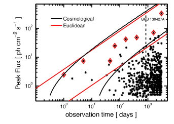
Figure 1: The Swift LGRB peak flux data from April 2005 to June 2013 plotted against observation-time. The plot illustrates how the probability of observing a bright event increases with observation-time, $T$. Successively brighter events - termed PEH data - are indicated by diamonds. A 90% confidence band constrains the data - this corresponds to the probabilities $\mathcal{P}=5\%$ (top) and $\mathcal{P}=95\%$ (bottom) of detecting at least one event within $T$. We see that the bright burst GRB 130427A is consistent with the prediction made in Howell et al. (2007a) (indicated by the vertical dashed line).

The basic concept is illustrated in Figure 1 which shows the Swift LGRB peak flux data plotted up to June 2013 against observation-time. Using a log-log plot it is apparent that successively brighter events have an observation-time dependence – the longer you observe, the greater the probability of observing an exceptionally bright event such as GRB 130427A. Successively brighter events are indicated by diamonds – these are the PEH data. The figure shows how PEH data is constrained using the Euclidean and cosmological log $P$– log $T$ models of (Howell et al., 2007b; Howell & Coward, 2013). One should note that the data is not always as well behaved – for example, there is always a possibility of a bright event occurring early in a time series. Therefore data extraction methods, which will be discussed later in Section 9, are employed to gain an optimal data set.

Adopting a time dependence allows the method to be used as a tool to predict the likelihood of future events. This is clearly illustrated in Figure 1. The vertical dashed line indicates the year 2007 when this relation was first published in Howell et al. (2007a) using a smaller sample of Swift bursts. We see that since this initial result two additional bursts consistent with the prediction have been added to the PEH sample. These include the recent bright burst GRB 130427A (Perley et al., 2014; Levan et al., 2013).

In this paper we will show that the log $z$– log $T$ relation can complement the more frequently used number count relations. As shown in Howell & Coward (2013), as PEH events approach the local low-$z$ regime rapidly, the GRB selection function (Coward, 2007) and high-$z$ selection effects such as the ‘redshift desert’ (Coward et al., 2008, 2013) have a negligible effect. Therefore, observation time relations can be used as a test of parameter compatibility without consideration of selection biases. To examine the LF of LGRBs, section 5 will extend previous studies by introducing a new cosmological log $L$– log $T$ relation.

3 The detection efficiency of Swift

Modeling the triggering criteria of an astronomical instrument can be critical and an oversimplified approach can lead to errors in the determination of population parameters or incorrect assumptions of the completeness of a sample. For instruments prior to Swift, such as BATSE, assuming a single detection threshold based on an increased photon count rate above background was a reasonable approximation (however, see Shahmoradi & Nemiroff, 2011, for further discussion of BATSE). However, for Swift a highly complex triggering algorithm has been adopted based on 674 different trigger criteria (see L14 for a comprehensive description).

Approximating the triggering response of such a sophisticated instrument as Swift is highly challenging. Numerous studies have approached this problem by assuming a single detection threshold based increased photon count rate above background (Le & Dermer, 2007; Guetta & Piran, 2007; Elliott et al., 2012; Salvaterra et al., 2012) (the sole triggering criterion used for BATSE), have used analytical approximations of the Swift triggering efficiency (Qin et al., 2010; Wanderman & Piran, 2010; Lu et al., 2012) or have adopted an effective threshold based on the luminosity-redshift distribution (Kistler et al., 2008; Cao et al., 2011b; Kistler et al., 2013).

In this study we use an alternative approach based on the recent comprehensive study of L14, who have mimicked the 674 criteria of the Swift triggering algorithm through a Monte Carlo approach. This included monitoring increased count rates on different timescales, energy bands and regions of the focal plane, periods of foreground (periods of strong emission) and background periods. Using BAT detected GRB light curves with redshifts, a mock rest frame sample was created and converted to photon counts corresponding to different incidence angles. Through a simulation of 50000 bursts, a detailed comparison of the triggered sample with the observed Swift distributions enabled both a thorough interrogation of the Swift detector response and a determination of the global parameters of the LGRB population.

To produce a set of efficiency functions for the Swift instrument we make use of the resulting L14 distributions (simulated and detected) in peak flux and redshift. This is a different approach to other studies which have determined similar functions based solely on the Swift detected distributions (Wanderman & Piran, 2010) or have used a simple scaling criteria (Howell & Coward, 2013). The adoption of these efficiency functions is important in this study. For example, the determination of a local rate density using the $V_{\mathrm{max}}$ method (see later section 10) uses only a small sample of the closest occurring bursts – in this scenario, the flux threshold of the detector has a highly significant bearing on the final estimate. The remainder of this section will present and describe the analytical forms of these functions.

3.1 The Swift peak flux efficiency function

Figure 2 shows the simulated and triggered peak flux sample of L14. The triggered sample is produced through a comprehensive reproduction of the Swift triggering algorithm. Although the simulated data was produced using a specific set of model parameters, we note the broad simulated distribution of peak fluxes (50,000) samples the detection response across a significantly wider range of values than generally considered. In comparison to the other techniques to model the Swift triggering algorithm, we suggest that the triggered sample (obtained through careful modeling of all 674 criteria) provides an adequate representation of the Swift response for use in this study.

By scaling of the simulated peak flux and triggered distributions of L14, we obtain the following trigger efficiency function:

$$\color[rgb]{0,0,0}\eta_{P}(P)=\frac{a(b+cP/P_{0})}{(1+P/d\,P_{0})}\,.$$ (1)

Within the range $5.87\times 10^{-9}$ $<P<$ $1.69\times 10^{-5}$ $\eta_{P}$ the function takes the parameters: {a = 0.47,; b = -0.05 ; c = 1.46 ; d = 1.45  $P_{0}=1.6\times 10^{-7}$}; below and above this range the function equals 0 and 1 respectively. The form of $\eta_{P}(P)$ is shown in Figure 3. We apply this function to the simulated peak flux population within the above range and are able to reproduce the triggered population of L14 with a statistical computability of $P_{\mathrm{KS}}>99\%$ as measured by a two sample Kolmogorov-Smirnov test.

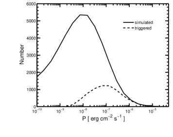
Figure 2: The simulated and triggered peak flux sample of L14 based on a comprehensive study of the Swift detection efficiency. The broad simulated distribution of peak fluxes (50,000) is able to sample the detection response across a wide range of values.

As discussed earlier, many studies use a simple Heaviside step function to account for the triggering threshold of Swift. For illustration Figure 3 compares $\eta_{P}(P)$ with two step function approximations: a value of 0.4 ph cm^-2 s^-1 similar to the value often adopted for BATSE; a value of 2.6 ph cm^-2 s^-1 used by Salvaterra et al. (2012) to produce a sample of bursts with a completeness of 95%. We see that even the higher of these two thresholds indicates a triggering efficiency of no more than 50%. It is apparent how the adoption of such approximations, or similar estimates based on an effective detection threshold determined from the luminosity-redshift plane, could be problematic when estimating the relative contributions of bright and dim bursts.

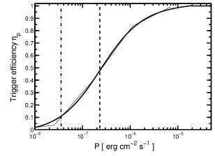
Figure 3: The triggering efficiency function of Swift as a function of peak flux for LGRBs adapted from the simulated sample of L14. The efficiency of the Swift trigger is shown by the thin line. Two Heaviside step function approximations are shown for comparison at values of 0.4 ph cm^-2 s^-1 and 2.6 ph cm^-2 s^-1.

3.2 The Swift redshift efficiency function

To model the efficiency as a function of redshift, z, we use the result of Fig. 16a of L14 to produce the following piecewise analytical fit:

$$\eta_{z}(z)=\biggl{\{}{\begin{array}[]{lll}a+b\,\mathrm{exp}(-z/c)&z\,<\,5.96\\ 0.02&z\,>\,5.96\\ \end{array}}$$ (2)

which takes the values {a = -0.01; b = 1.02; c = 1.68}. We note that this function provides the fraction of bursts at each redshift interval that have passed the peak flux triggering criteria; therefore, if working in solely redshift space – such as when using the log $z$– log $T$ distribution in section 10 – one should also scale the rate with the average peak flux efficiency of 14% determined by L14.

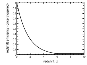
Figure 4: The redshift efficiency curve for Swift adapted from Fig 16a of L14. The figure represents the detection efficiency as a function of redshift.

We will apply these functions in our analysis of the Swift data sample – it will be interesting to draw comparisons between the global parameters determined in this study with those determined through simulation of the Swift response by L14.

4 Theoretical Framework

4.1 GRB Flux and luminosity relations

An isotropic equivalent luminosity in the source frame (erg s^-1) can be calculated from:

$$L=4\pi d_{\mathrm{L}}(z)^{2}P\frac{k(z)}{b}$$ (3)

where $P$ is the energy flux (erg s^-1 cm^-2) in the observed energy band $E_{\mathrm{min}}<E<E_{\mathrm{max}}$, $d_{\mathrm{L}}(z)$ is the luminosity distance and $k(z)$ and $b$ are correction terms to convert the observed flux in the detector band (for Swift this is 15–150 keV) to the rest frame band 1–$10^{4}$ keV . The first of these correction terms is the bolometric correction $b$ which accounts for the differing fraction of gamma ray energy seen in the detector band (Imerito et al., 2008; Wanderman & Piran, 2010):

$$b=\int^{E_{\mathrm{max}}}_{E_{\mathrm{min}}}ES(E)dE/\int^{10000}_{1}ES(E)dE\,,$$ (4)

where $S(E)$ is the rest-frame photon spectrum (ph cm^-1 keV^-1) multiplied by a factor of $E$ (energy in keV) as part of the conversion to energy units. The term $k(z)$ the cosmological $k$-correction and given by:

$$k(z)=\int^{E_{\mathrm{max}}}_{E_{\mathrm{min}}}ES(E)dE/\int^{E_{\mathrm{max}}(1+z)}_{E_{\mathrm{min}}(1+z)}ES(E)dE\,.$$ (5)

Rearranging and substituting for $b$ and $k(z)$ in the above equation yields the familiar relation for energy flux:

$$P=\frac{\int^{(1+z)E_{\mathrm{max}}}_{(1+z)E_{\mathrm{min}}}ES(E)\mathrm{d}E}{4\pi d_{\mathrm{L}}(z)^{2}}\,.$$ (6)

For long duration GRBs the function $S(E)$ is typically modeled by a Band function (Band, 2003) which we use with high and low energy spectral indices of -2.25 and -1 and a peak energy of 511 keV (in the source frame). Unless spectral forms and parameters are available (such as those used in determining the luminosity corrections in section 8) we will assume these values.

4.2 GRB Luminosity Function

To model the LGRB Luminosity Function (LF), we use a Broken Power law model (BPL) model which takes the form:

$$\Phi(L)\propto\biggl{\{}{\begin{array}[]{ll}\hskip 2.84526pt\left(L/L_{*}\right)^{\alpha}\hskip 8.53581ptL<L^{*}\\ \hskip 2.84526pt\left(L/L_{*}\right)^{\beta}\hskip 8.53581ptL\geq L^{*}\\ \end{array}}$$ (7)

with, $L$ is the isotropic rest frame luminosity in the 1-10000 keV energy range and $L_{*}$ a characteristic cutoff scaling that separates the two slopes $\alpha$ and $\beta$. The additional power law in comparison with single power law forms LF allows to examine the low and high luminosity parts of the distribution. We follow the studies of Meszaros & Meszaros (1996, 1995); Reichart & Meszaros (1997); Butler et al. (2010) and assume no luminosity evolution with redshift.

4.3 GRB source rate evolution

To obtain a source rate evolution model for LGRBs with redshift, $R_{\rm GRB}(z)$, we use the piecewise function of Wanderman & Piran (2010):

$$\color[rgb]{0,0,0}R_{\mathrm{GRB}}(z=0)=\biggl{\{}{\begin{array}[]{lll}(1+z)^{a}&z\,<\,z_{*}\\ (1+z_{*})^{a-b}(1+z)^{b}&z\,>\,z_{*}\\ \end{array}}$$ (8)

with values of $z_{*}=3.6$, a=2.1 and b=-0.7 based on the recent study of W14.

4.4 The all sky event rate equation of GRBs

The number of GRBs per unit time within the redshift shell $z$ to $z+\mathrm{d}z$ with luminosity $L$ to $L+\mathrm{d}L$ is given by:

$$\frac{\mathrm{d}N}{\mathrm{d}t\mathrm{d}z\mathrm{d}L}\hskip 1.42262pt=\psi(z)\frac{\mathrm{d}V(z)}{\mathrm{d}z}\frac{R_{\mathrm{GRB}}(z)}{(1+z)}\,\mathrm{d}z{\hskip 1.42262pt}\Phi(L)\,.\vspace{0mm}$$ (9)

Here the $(1+z)$ factor accounts for the time dilation of the observed rate by cosmic expansion; its inclusion converts source-count information to an event rate. The co-moving volume element:

$$\frac{\mathrm{d}V}{\mathrm{d}z}=\frac{4\pi c}{H_{0}}\frac{d_{\mathrm{\hskip 0.7113ptL}}^{\hskip 4.2679pt2}(z)}{(1+z)^{\hskip 0.7113pt2}\hskip 1.42262pth(z)}\,,$$ (10)

describes how the number densities of non-evolving objects locked into Hubble flow are constant with redshift. The quantity $h(z)$, is the normalized Hubble parameter,

$$h(z)\equiv H(z)/H_{0}=\big{[}\Omega_{\mathrm{m}}(1+z)^{3}+\Omega_{\mathrm{\Lambda}}\big{]}^{1/2}\,,$$ (11)

where $\Omega_{\mathrm{m}}+\Omega_{\mathrm{\Lambda}}=1$ (for further details see Carroll et al., 1992). For a ‘flat-$\Lambda$’ cosmology, we employ the most recent cosmological parameters measured by Planck of $\Omega_{\mathrm{m}}=0.32$, $\Omega_{\mathrm{\Lambda}}=0.68$ and $H_{0}=67$ km s^-1 Mpc^-1 for the Hubble parameter at the present epoch (Planck Collaboration et al., 2013).

5 The log $L$–log $T$ relation

From equation 9, the rate of GRBs with a peak luminosity greater than $L$ observed by an instrument with sky coverage $\Omega$ is given by:

$$\dot{N}(>L)=\frac{\Omega}{4\pi}\int\limits_{\hskip 11.38109ptL_{\mathrm{min}(z)}}^{\hskip 11.38109pt\infty}\Phi(L)\mathrm{d}L\int\limits_{\hskip 2.84526pt0}^{\hskip 11.38109pt\infty}\frac{\mathrm{d}V(z)}{\mathrm{d}z}\frac{R_{\mathrm{GRB}}(z)}{(1+z)}\,\mathrm{d}z\,,\vspace{0mm}$$ (12)

were $L_{\mathrm{min}}(z)=\mathrm{max}[L,L(p_{\mathrm{min}},z))]$: here $L(P_{\mathrm{min}},z)$ is obtained through equation 6 and is the minimum luminosity required by a burst at redshift $z$ to produce a peak flux of $P_{\mathrm{min}}$. This equation was used by Salvaterra et al. (2009) to estimate the number of bursts with peak luminosity $>10^{53}$ in the Swift sample.

To introduce an observation-time dependence, $T$, we follow the probability event horizon concept of Coward & Burman (2005) and note that as GRBs are independent of each other, their observation-times will follow a Poisson distribution in time. Therefore, the temporal separation between events will follow an exponential distribution defined by a mean number of events, $\dot{N}(>L)\,T$. The probability $\mathcal{P}$ for at least one event $>L$ is given by:

$$\mathcal{P}(n\geq 1;\dot{N}(>L),T)=1-e^{-\dot{N}(>L)T}=\mathcal{P}\,.$$ (13)

For this equation to remain satisfied with increasing observation-time:

$$\dot{N}(>L)T=|\mathrm{ln}(1-\mathcal{P})|\,.$$ (14)

Equating the above equation for $L$ and $T$ we obtain a relation for the evolution of isotropic luminosity as a function of observation-time. By setting $\mathcal{P}$ to some arbitrary value, log $L$– log $T$ curves can be obtained numerically through equations 12 and 14. Following Howell & Coward (2013); Howell et al. (2007b, a) one can plot upper and lower thresholds by setting $\mathcal{P}=(0.95;0.05)$ – we will refer to these curves as 90% PEH bands.

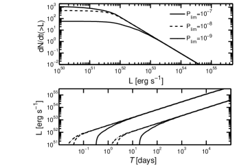
Figure 5: The functions $\dot{N}(>L)$ (top panel) and log $L$– log $T$ (lower panel) for the same model parameters but using different values of $P_{\mathrm{min}}$. The flux limit has little effect on the $\dot{N}(>L)$ above $10^{53}$ erg s^-1 – for the upper log $L$– log $T$ 90% PEH threshold (which gives the 5% peak luminosity probability within time $T$) this corresponds to around 4 days of observation time.

We note that equation 12 is dependent on an estimate of $P_{\mathrm{min}}$ for the lower limit of the integral over the LF. As shown in section 3 it is difficult to model the Swift detection efficiency through a single value of $P_{\mathrm{min}}$. We find however, that the log $L$– log $T$ circumvents this obstacle through its dependence on the most luminous events. Figure 5 illustrates this property by comparing the functions $\dot{N}(>L)$ (top panel) and log $L$– log $T$ (lower panel) models for the same parameters but using different values of $P_{\mathrm{min}}$. The flux limit has little effect on the $\dot{N}(>L)$ above $10^{53}$ erg s^-1 – for the upper log $L$– log $T$ 90% PEH threshold this corresponds to around 4 days of observation time, equal to that of the first PEH data point used in this study( see later in table 2). We find similar convergence of the log $L$– log $T$ curves for rates within 0.2-0.9 Gpc^-3yr^-1 We therefore use a value of $P_{\mathrm{min}}=10^{-8}$ erg s^-1cm^-2 noting that the adoption of this value will not influence our results.

6 The log $z$– log $T$ relation

One can extend the arguments of the previous section to derive a log $z$– log $T$ relation (Howell & Coward, 2013). From equation 9 the rate of GRBs observed by an instrument with sky coverage $\Omega$ within a redshift limit $z_{\rm{L}}$ is given by:

$$\vspace{6mm}\dot{N}(<z_{\rm{L}})=\frac{\Omega}{4\pi}\int\limits_{\hskip 34.1433ptL_{\mathrm{min}}(\mathrm{P_{min}},z_{\mathrm{L}})}^{\hskip 19.91692ptL_{\mathrm{max}}}\Phi(L)\,\mathrm{d}L\int\limits_{0}^{\hskip 14.22636ptz_{\rm{L}}}\frac{\mathrm{d}V(z)}{\mathrm{d}z}\frac{\eta_{z}(z)\,R_{\mathrm{GRB}}(z)}{(1+z)}\,\mathrm{d}z\,,\vspace{-2mm}$$ (15)

with $z_{\mathrm{L}}$ obtained by applying the value, $P_{\mathrm{min}}$, to equation 6; the quantity $\eta_{z}$ is the efficiency of obtaining a redshift (sub-section 3.2).

A similar argument as that used to determine equation 14, yields the following relation for the temporal evolution of redshift:

$$\dot{N}(<Z_{\rm{L}})T=|\mathrm{ln}(1-\mathcal{P})|.\\$$ (16)

This equation can be equated for $T$ and $z$ to set a spatial dependence on GRB populations. Curves of log $z$– log $T$ for $\mathcal{P}=(0.95;0.05)$ can be obtained numerically through equations 15 and 16. As before, these will be referred to as 90% PEH bands.

As shown above, the log $z$ –  log $T$ and log $L$ –  log $T$ relations are derived seamlessly from standard integral distributions. Thus, model parameters obtained by fitting to a differential brightness distribution should satisfy the two observation-time relations presented above (equations 14 and 16).

An advantage of this technique is that the PEH sample in redshift space is predominantly from the closest events. Therefore consideration of high-$z$ selection bias is not essential. We will use log $z$ – log $T$ relation later in section 10 to validate our estimate of (beaming uncorrected) local rate density, $\rho_{0}$.

7 The log $L$–log $T$ relation as a probe of the LGRB luminosity function

Figure 6 shows how the log $L$–log $T$ 90% PEH bands can indicate of the form of the LF. For illustration we adopt an arbitrary broken power law LF with parameters: $L_{*}=5\times 10^{51}\,\mathrm{erg}\mathrm{s}^{-1},\alpha=-0.5$ and $\beta=-2.3$. This LF is shown in panel (A) and the corresponding log $L$–log $T$ curve is shown the other panels as a shaded component. Solid and dashed lines in each of the panels B-D illustrate how the log $L$ –  log $T$ curves are modified by changing one of the parameters of the LF. Below, we discuss and provide physical interpretations for these changes:

• Panel (B) shows that increasing/decreasing the value of the break Luminosity ($5\times L_{*};0.5\times L_{*}$) produces a vertical increase/decrease of the log $L$–log $T$ curves. A higher value of $L_{*}$ results in a greater probability of a bright event; thus an increased probability of a more energetic event at early observation times.

• Panel (C) shows that increasing/descreasing the gradient of the low end slope through $\alpha$ offsets the curves in the positive/negative horizontal direction. Increasing $\alpha$ produces a greater proportion of dimmer bursts - therefore, a lower probability and thus, an increased waiting time, for a high luminosity event.

• Panel (D) illustrates how increasing/descreasing the value of $\beta$ produces a gradient change. A flatter value of the bright-end slope produces a greater proportion of bright burst; this corresponds with an increase in the gradient of the probability curves.

The sensitivity of the log $L$–log $T$ PEH curves to the parameters ($L_{*}$  $\alpha$, $\beta$), means that estimates obtained through a brightness distribution (log $N$–log $P$) can be validated. In particular, employing this complementary method can help to untangle degeneracies that are encountered in using a log $N$–log $P$ fit. Before we conduct our analysis, in the next two sections we will describe the LGRB data sample and then discus how to extract a PEH data set.

8 The LGRB Data Sample

8.1 The redshift data sample

In recent studies Zhang (2011) and Bromberg et al. (2012) have suggested that the $T_{90}=2\,\mathrm{s}$ division of short and long GRBs based on the BATSE bimodial distribution (Kouveliotou et al., 1993) is a detector dependent categorisation and therefore not appropriate for Swift bursts. Other studies have suggested an intermediate duration class of bursts between these two classes (Horváth et al., 2010). Additionally sub-luminous GRBs (SL-GRBs; Howell & Coward, 2013; Virgilii et al., 2008; Imerito et al., 2008; Daigne & Mochkovitch, 2007; Cobb et al., 2006; Coward, 2005) and short GRBs with extended emissions (SGRB-EEs; Norris et al., 2011)) have been suggested to be members of sub-populations of burst.

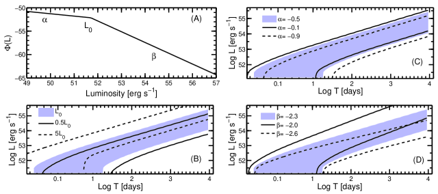
Figure 6: Panel A shows the broken power law LF model adopted for this study. For illustration we adopt the parameters $L_{*}=5\times 10^{51}\,\mathrm{erg}\mathrm{s}^{-1},\alpha=-0.5$ and $\beta=-2.3$. The shaded portions of each of the remaining panels show the log $L$ – log $T$ 90% PEH bands corresponding to these parameters - the upper and lower curves in each case correspond with the probabilities given Figure 1. The solid and dashed lines in the panels B–D show how the curves are modified by changing each of the parameters: $L_{*}$, $\alpha$ and $\beta$. Panel B: increasing/decreasing the value of the break Luminosity, $L_{*}$, results in a vertical increase/decrease of the log $N$–log $L$ curve. Panel C: increasing/descreasing the low end slope represented by $\alpha$ shifts the curves in the positive/negative horizontal direction. Panel (D) increasing/descreasing the value of the high end slope ($\beta$) produces a gradient change.

To obtain a selection of Swift LGRBs, rather than employing a $T_{90}$ cut, we use the catagorisations given in the Jochen Greiner online catalogue (JG) of well localized GRBs . As the burst catagorisations and redshifts in this catalogue are subject to review through follow up studies we find it a useful resource to isolate a LGRB sample (for example, the catalogue was recently updated using 15 new redshifts from the TOUGH survey Hjorth et al., 2012).

We use data up to June 2013 which includes 232 redshifts of which 209 have secure redshifts (uncertain redshifts were omitted). To arrive at the redshift sample given above we have excluded three SL-GRBs, 060218, 060505 and 100316D (see Howell & Coward (2013) for further discussion of these bursts), 7 bursts catagorised as SGRB-EEs (all but one have $T_{90}>2\,\mathrm{s}$) (Norris et al., 2011) and 3 bursts (101225A, 111209A & 121027A) strongly suggested to be part of an ultra-long GRB population (Gendre et al., 2013; Levan et al., 2014; Stratta et al., 2013).

Figure 7 shows the sample of 209 bursts with redshifts determined through emission, absorbtion and photometry. For redshifts determined though multiple criteria, absorbtion takes precedence followed by photometry. The histograms show that photometrically determined bursts are detected almost uniformly across redshift, while host galaxy emission spectra cover a limited range $0.3<z<2.8$. From our sample of 209 redshifts we select the 175 bursts obtained through absorbtion spectra (162 of the sample; or 78%) or photometrically $(13;6\%)$. A two sample Kolmogorov-Smirnov test (KS) shows these two samples to be compatible at the KS probability $P_{\mathrm{KS}}=22\%$ level. We follow Wanderman & Piran (2010) and omit the sample of redshifts obtained through host galaxy emission spectra which, due to their narrow redshift range, are not statistically compatible with the absorbtion sample $(P_{\mathrm{KS}}\sim 10^{-3}\%$).

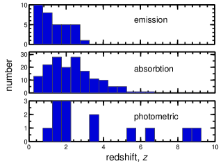
Figure 7: The redshift distributions of Swift observed LGRBs up to June 2013 separated into data obtained though absorbtion and emission spectroscopy and photometrically. The photometric redshift distribution is approximately uniform across the observed range. In comparison, the sample obtained through host galaxy emission spectra are only observed within a limited range $0.3<z<2.8$.

8.2 Luminosity data

To calculate isotropic peak luminosity data, $L$, from the redshift sample we use equations 3 – 5. Peak energy flux data is taken from Butler’s online catalogue of Swift BAT Integrated Spectral Parameters . This catalogue, an extension of the work presented in Butler et al. (2007); Butler et al. (2010), has circumvented the nominal BAT upper energy of 150 keV to produce accurate values of $E_{\mathrm{iso}}$ through a novel Bayesian approach. Peak spectral energies from the BATSE catalogue have been used to set a strong prior on the range of GRB model parameters specified by one of three models of increasing complexity: a simple power law, a power law times an exponential cutoff and a Band function (Band et al., 1993). The resulting spectra were shown to be in agreement with observations from satellites operating at much broader energy ranges e.g. Konus-Wind (10–770 keV) and Suzuku (0.3–-600 keV). We use the spectral parameters catalogued for each burst to calculate the $k$ and bolometric correction terms given in section 4.1.

Figure 8 shows the sample of 209 burst luminosities using the redshifts determined through emission, absorbtion and photometry. As expected, the sample obtained through host galaxy emission spectra are clearly biased towards lower values of luminosity. This observation is confirmed through a KS test in which a value of $P_{\mathrm{KS}}\sim 1\%$ is obtained between the absorbtion and emission samples. The photometric sample are compatible with the emission sample at a level of $P_{\mathrm{KS}}=23\%$ and are therefore included in our final sample of 175 bursts. Our full data sample is shown in Table LABEL:table_lum_data and is available online.

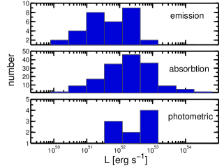
Figure 8: The peak luminosity distributions of Swift observed LGRBs up to June 2013 obtained using absorbtion and emission spectroscopy as well as photometrically. The sample obtained through host galaxy emission spectra are clearly biased towards lower values of luminosity.

Figure 9 shows the luminosity–redshift distribution (filled stars). The sample determined through emission spectra are also shown (unfilled stars). We test the statistical compatibility of our samples using a 2D-KS (Peacock, 1983; Fasano & Franceschini, 1987) test in the $L_{\mathrm{iso}}$–$z$ plane. For the absorbtion/photometric samples we obtain $(P_{\mathrm{KS,2d}}\sim 17\%)$ signifying good compatibility. The decision to omit emission data is further justified through a value of $(P_{\mathrm{KS,2d}}\sim 10^{-3}\%)$ for the absorbtion/emission data samples.

In the next section we will outline the extraction procedure used to obtain PEH data. We will then be well equipped to constrain this data using both log $z$ –  log $T$ and log $L$ –  log $T$ 90% PEH bands.

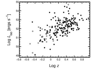
Figure 9: The luminosity–redshift distribution of Swift LGRBs shown as filled black stars. The bursts with redshifts determined through emission spectra are shown by unfilled stars - these bursts are predominantly at lower-$z$.

9 Data extraction methodology

To extract PEH data, we follow the FromMax method used by Howell & Coward (2013) to untangle different populations of the Swift GRB sample. This invoked the temporal cosmological principle: for time scales that are short compared to the age of the Universe, there is nothing special about the time we switch on our detector. Therefore, the time-series can be treated as closed loop, i.e. the start and endpoints of the time series can be joined and the start time set immediately after the brightest event. Successively brighter/closer events and their observation-times are then recorded to produce a PEH data set.

Employing this technique circumvents the possibility of a bright event occurring early in a time series; this would minimize the amount of output data as the next largest event would most probably occur near the end of the time series. Such a situation could be encountered through a detector with a high energy cutoff – if a large number of events have energies around the threshold value a bias could be introduced.

Another feature of the FromMax method is that it establishes the total time duration of the PEH output to be equivalent to that of the total observation-time – this ensures a well ordered data sample is produced with a consistent time signature. Howell & Coward (2013) showed through statistical testing that the improved data set retains the statistical signature of the original.

To apply the procedure to a sample of $L(T)$ time-series data, we first define the brightest event by $L_{*}$ with an observation-time stamp $T_{*}$ and denote the time of the last, most recent occurring event, as $T_{\mathrm{max}}$. Treating the data as a closed loop we reorder the data starting from the first event after $L_{*}$. The time stamps of the re-ordered data set $L^{\backprime}(T_{L}^{\backprime})$ are now defined as:

$$T^{\backprime}_{L}=\biggl{\{}{\begin{array}[]{lll}T-T_{*}&T>T_{*}\\ \\ T+T_{\mathrm{max}}-T_{*}&T\leq T_{*}\end{array}}$$ (17)

In Howell & Coward (2013), to obtain a PEH data set the data was extracted from the first minimum $L_{\mathrm{min}}^{\backprime}=P_{i}^{\backprime}<L_{i+1}^{\backprime}$ – this additional step was to minimise the effect of an early bright event. In this study we adopt a simpler approach; we take the first PEH event as the first above or equal to the median value of the sample $L_{\mathrm{med}}$. A PEH data set is then obtained by recording successively brighter events $(L_{i}^{\backprime},T_{L,i}^{\backprime})$ satisfying the condition $L_{i+1}^{\backprime}>L_{i}^{\backprime}$ for $L_{i}^{\backprime}\geq L_{\mathrm{med}}^{\backprime}$.

To determine the PEH data set in the redshift domain one applies similar principles, treating the data as a closed loop but re-ordering the data from the first event after the closest redshift event $Z_{0}$. The time-stamps for the re-ordered set $Z^{\backprime}(T^{\backprime}_{Z})$ are then given by:

$$T_{Z}^{\backprime}=\biggl{\{}{\begin{array}[]{lll}T-T_{0}&T>T_{0}\\ \\ T+T_{\mathrm{max}}-T_{0}&T\leq T_{0}\end{array}}$$ (18)

A PEH data set is obtained by extracting data from the first event equal to or less than the median value of the distribution $Z_{\mathrm{med}}$, recording successively closer events $(Z_{i}^{\backprime},T_{Z,i}^{\backprime})$ satisfying the condition $Z_{i+1}^{\backprime}<Z{i}^{\backprime}$ for $Z_{i}^{\backprime}\geq Z_{\mathrm{med}}^{\backprime}$.

10 Constraining the rate density of Swift LGRBs

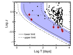
Figure 10: The log $z(T)$ distribution of Swift LGRBs up to August 2013 using redshifts obtained through absorbtion spectroscopy or photometrically – PEH data is indicated by the red diamonds. The median value for the distribution is shown by the horizontal dashed line. log $z$–log $T$ curves are used to support our rate estimates of $\rho_{0}=0.48^{+0.38}_{-0.24}$ Gpc^-3yr^-1 obtained through a $V_{\mathrm{max}}$ analysis. The shaded region represents the best estimate and thin dashed and solid curves show the lower and upper limits respectively. In each case the upper log $z$–log $T$ curve represents the 95% confidence threshold of at least 1 occurrence within an observation time $T$. The lower log $z$–log $T$ curve indicates the 95% confidence threshold of no occurrence occurring within $T$. We ignore the first PEH event in our analysis which occurred above the median threshold.

10.1 $V_{\mathrm{max}}$ analysis of the LGRB sample

As an initial estimate of $\rho_{0}$, the intrinsic beam uncorrected rate of LGRBs, we use the 9 LGRBs from the Swift sample which have been recorded within a volume encompassed by $z=0.6$ ( $\sim$ 3.7 Gpc). Extending Guetta & Della Valle (2007); Coward et al. (2012); Howell & Coward (2013) one can determine the rate through the maximum detection volumes of the sample:

$$\rho_{0}=\sum_{i}^{\in z_{i}\leq 0.6}\frac{1}{V_{\rm{max},i}}\frac{1}{T}\frac{1}{\Omega}\frac{1}{\eta_{z,i}}\frac{1}{\eta_{P,i}}$$ (19)

Here, $V_{\mathrm{max}}$ is the maximum volume out to which each burst could be detected, $T$ is the maximum observation-time for the sample, $\Omega$ is the sky coverage (1.33/4$\pi$).

The $V_{\mathrm{max}}$ method is highly sensitive to the value of the detector threshold – this poses a problem when considering detectors with highly complex triggering mechanisms such as Swift. To take into account the triggering efficiency for each individual burst, we first set a maximum flux limit of the detector by $6\times 10^{-9}\,\mathrm{erg}\,\mathrm{sec}^{-1}$, the minimum value for over 99% of the Swift LGRB sample, then weight each burst using the efficiency functions $\eta_{P}$ and $\eta_{z}$ from sections 3.

GRB	$z$	Peak Flux	$\eta_{P}$	$\eta_{z}$
		$(10^{-6}\mathrm{erg}\,\mathrm{sec}^{-1}\,\mathrm{cm}^{-2})$
060729	0.54	0.074	0.22	0.73
081007	0.53	0.18	0.42	0.73
090424	0.54	5.4	0.95	0.73
090618	0.54	2.6	0.91	0.73
101219B	0.55	0.099	0.28	0.73
120714B	0.4	0.017	0.045	0.79
130215A	0.6	0.12	0.33	0.7
130427A	0.34	30	0.99	0.82

Table 1: The data used to determine the rate of LGRBs from the Swift sample using the $V_{\mathrm{max}}$ method.

Table 1 outlines the values of redshift and peak flux for each of the bursts within $z=0.6$ and their relative scaling values, $\eta_{P}$ and $\eta_{z}$. We obtain a rate estimates of $\rho_{0}=0.48^{+0.38}_{-0.24}$ Gpc^-3yr^-1 where the errors are the 95% Poisson confidence limits (Gehrels, 1986).

We note that for this calculation will have ignored evolution effects within $z=0.6$. One can estimate the magnitude of any bias from this assumption by estimating a cosmic event rate:

$$\mathrm{d}R=\frac{\mathrm{d}V}{\mathrm{d}z}\frac{R_{\mathrm{GRB}}(z)}{1+z}\mathrm{d}z\,.$$ (20)

for two scenarios: a source rate evolution given by equation 8; a constant evolution $R_{\mathrm{GRB}}(z)=1$. As shown by Figure 11, out to $z=0.6$ the two curves differ by around a factor of 2. Therefore, in our later calculations we will examine the LF across a large enough range around the above estimate to allow for any possible offset.

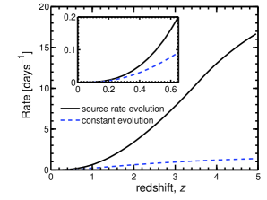
Figure 11: A comparison of the event rate of cosmic events using two different scenarions: an evolution based on LGRBs using equation 8; a constant cosmic evolution. We see that within $z=0.6$ the two curves differ by a factor 2.

10.2 The log $z$– log $T$ distribution

To test the validity of the $V_{\mathrm{max}}$ method we produce log $z$–log $T$ curves corresponding to the estimated rate $\rho_{0}=0.48^{+0.38}_{-0.24}$. Figure 10 shows the log $z$–log $T$ curves along with the log $z(T)$ distribution of Swift LGRBs – $z(T)$ PEH data is indicated by red diamonds. The median value for the distribution is shown by the horizontal dashed line. We note that we have excluded the first occurring PEH event in this analysis – GRB 090424 (z = 2.78). This event occurred above the median threshold and by our data extraction criteria discussed in section 9 - the rare events from the tail of the distribution occur well within this value.

The log $z$–log $T$ curves are constructed using an observed rate, obtained by scaling $\rho_{0}$ by a value of 0.14 which represents the triggering efficiency of Swift (Lien et al., 2014) and by the mean value of $\eta_{z}$ for our $V_{\mathrm{max}}$ sample which within $z=0.6$ equals 0.75.

The shaded region represents the best estimate and the thin dashed and solid curves show the lower and upper limits of $\rho_{0}$ respectively. In each case the upper log $z$–log $T$ curve represents the 95% confidence threshold of at least 1 occurrence within an observation time $T$. The lower log $z$–log $T$ curve indicates the 95% confidence threshold of no occurrence occurring within $T$. The PEH data is clearly constrained within the 90% threshold defined by the two sets curves supporting the estimate of $\rho_{0}$ obtained through the $V_{\mathrm{max}}$ method.

11 Constraining the LF of LGRBs

In this section we estimate the most compatible fitting parameters for the LGRB LF {$\alpha$, $\beta$ and $L_{*}$ } within the range $0.2<\rho_{0}<1$ Gpc^-3yr^-1. We will use both the log $L$ – log $T$ 90% PEH bands and $\chi^{2}$ fitting of the log $N$– log $P$ distribution in an iterative procedure over $\rho_{0}$. We will firstly describe our procedure after which we will present our results.

11.1 Constraining the LGRB LF through the log $L$ – log $T$ distribution

To place constraints on the parameters of the LF before log $N$– log $P$ fitting is performed, the parameters {$\rho_{0}$, $\alpha$, $\beta$ and $L_{*}$} are required to constrain $L(T)$ data through log $L$ – log $T$ 90% PEH bands. The data is obtained by applying the methodology described in section 9. The log $L$ – log $T$ data is given in Table 2.

Using each set of {$\rho_{0}$, $\alpha$, $\beta$ and $L_{*}$} we construct log $L$ – log $T$ 90% PEH bands. A measure of compatibility is obtained through the binomial maximum likelihood (BML) (BML; Johnson et al., 1993) estimate for obtaining data within the 90% bands – a larger value signifies a good fit to the data; in this procedure a BML estimate of 88% (1 failure in 8) will indicate a compatible set of parameters.

GRB	$T_{\mathrm{obs}}$	Peak Luminosity	Peak Flux	$z$
	(days)	$(10^{53}\mathrm{erg}\,\mathrm{sec}^{-1}\,)$	$(10^{-7}\mathrm{erg}\,\mathrm{sec}^{-1}\,\mathrm{cm}^{-2})$
130514A	4.00	0.37	1.60	3.60
130606A	26.00	3.09	1.85	5.91
050401	140.00	4.92	9.73	2.90
061007	691.00	5.73	15.52	1.26
071020	1069.00	6.67	9.02	2.15
080607	1301.00	17.97	17.63	3.04
080721	1345.00	25.43	18.89	2.59
130505A	3088.00	30.29	18.93	2.27

Table 2: The $L(T)$ data sample used to constrain the LF parameters.

11.2 The log N-log P brightness distribution for Swift GRBs

To perform $\chi^{2}$ minimisation of the log $N$– log $P$ brightness distribution of Swift LGRBs we use 15-150 keV band peak energy flux data from Butler’s online catalogue of Swift BAT Integrated Spectral Parameters described in section 8. From equation 9 one can define a differential log $N$– log $P$ relation (Kommers et al., 2000; Porciani & Madau, 2000; Salvaterra & Chincarini, 2007; Campisi et al., 2010; Howell & Coward, 2013) which is the observed rate of bursts within a peak flux interval ($P_{1}$, $P_{2}$):

$$\dot{N}(P_{1}\leq P<P_{2})=\frac{\Omega\,\eta_{P}(P)}{4\pi}\int\limits^{\hskip 8.53581pt\infty}_{\hskip 5.69054pt0}\frac{\mathrm{d}V(z)}{\mathrm{d}z}\frac{R_{\mathrm{GRB}}}{(1+z)}\mathrm{d}z\int\limits^{\hskip 19.91692ptL(P_{2},z)}_{\hskip 17.07164ptL(P_{1},z)}\Phi(L)\mathrm{d}L\,,$$ (21)

with ${L(P_{1,2},z)}$ obtained through equation 3. The peak flux triggering efficiency $\eta_{P}$ is given in equation 1 (section 3.1).

We bin peak flux data into logarithmically spaced intervals $\Delta P$ and ensure each bin contains at least 5 bursts (Wall et al., 2003). Bursts per bin $\Delta N$ and their uncertainties $\pm\sqrt{\Delta N}$ are converted into burst rates $\Delta R$ by dividing by the live time of the search $\Delta T$ (Kommers et al., 2000). The peak flux intervals, number of bursts and burst rates data used for the fit is given in Table 3.

The goodness of fits are indicated through values of minimum $\chi^{2}$ per degree of freedom, $\chi^{2}/dof$, and $P_{\chi^{2}}$. The latter parameter is the probability of obtaining a $\chi^{2}$ value equal to or greater than $\chi^{2}$ given the data is drawn from the model using the best-fit parameters.

11.3 Parameter Search

For each value of $0.2\leq\rho_{0}\leq 1.0$ we iterate through a range of LF parameters {$L_{*}$, $\alpha$ and $\beta$} to construct log $L$ – log $T$ 90% PEH bands. If the BML estimate for obtaining data within the 90% bands is $\geq$ 88% (1 failure in 8) we perform $\chi^{2}$ minimisation of the log $N$– log $P$ and store the value of $\chi^{2}$. We continue until a maximum $\chi^{2}$ is obtained.

P1	P2	$\dot{N}$	$\Delta\dot{N}/\Delta P$
$\mathrm{erg}\,\mathrm{s}^{-1}\,\mathrm{cm}^{-2}$	$\mathrm{erg}\,\mathrm{s}^{-1}\,\mathrm{cm}^{-2}$	$\mathrm{yr}^{-1}$	$\mathrm{yr}^{-1}\,\mathrm{erg}\,\mathrm{s}\,\,\mathrm{cm}^{2}$
$\times 10^{-7}$	$\times 10^{-7}$		$\times 10^{5}$
0.062	0.10	0.94	232
0.10	0.17	3.10	455
0.17	0.28	7.90	707
0.28	0.47	9.20	497
0.47	0.77	11.00	369
0.77	1.30	11.00	225
1.30	2.10	12.00	144
2.10	3.50	7.20	51.70
3.50	5.80	3.60	15.90
5.80	9.60	4.00	10.50
9.60	16.00	1.80	2.80
16.00	26.00	1.50	1.46
26.00	44.00	0.47	0.27
44.00	330.00	0.71	0.025

Table 3: The data used to fit the differential peak flux distribution of the Swift long GRB sample. The data is obtained within the energy range 15-150 keV.

11.4 Results

Table 4 shows global LGRB parameters that satisfied the conditions of the parameter search (indicated by a $\checkmark$). We also show a few values each side of this range obtained by relaxing the selection criteria (indicated by a X).

We found that parameters that passed both selection criteria were within the range $0.5\leq\rho_{0}\leq 0.8$. For values outside this range, steeper values of $\beta$ were required to fit the log N–log P distribution. However, as discussed in section 7, steep values of $\beta$ correspond with a lower proportion of bright bursts, resulting in log $L$ – log $T$ curves that are too flat at the high $L$ end to constrain the brightest bursts.

Values of $\rho_{0}$ greater than 0.8  $\mathrm{Gpc}^{-3}\,\mathrm{yr}^{-1}$ fared better than values below 0.5  $\mathrm{Gpc}^{-3}\,\mathrm{yr}^{-1}$ which were ruled out by poorly constrained $L(T)$ PEH data (as shown, values of MLE=0.75 were obtained for 0.85-0.90  $\mathrm{Gpc}^{-3}\,\mathrm{yr}^{-1}$).

$\rho_{0}$	$L_{*}$	$\alpha$	$\beta$	$\chi^{2}/dof$	$P_{\chi^{2}}$	BML	Pass/Fail
$\mathrm{Gpc}^{-3}\,\mathrm{yr}^{-1}$	$\times 10^{52}\mathrm{erg}\,\mathrm{sec}^{-1}$
$0.90$	$0.95\pm 0.80$	$-1.15\pm 0.10$	$-2.66\pm 1.83$	1.538	13.41	0.75	X
$0.85$	$0.92\pm 0.79$	$-1.10\pm 0.10$	$-2.66\pm 1.84$	1.525	14.05	0.75	X
$0.80$	$0.80\pm 0.43$	$-0.95\pm 0.09$	$-2.59\pm 0.93$	1.239	33.04	0.88	$\checkmark$
$0.75$	$0.81\pm 0.56$	$-0.93\pm 0.11$	$-2.60\pm 1.24$	1.242	32.74	0.88	$\checkmark$
$0.70$	$0.70\pm 0.26$	$-0.80\pm 0.10$	$-2.55\pm 0.67$	1.272	30.32	0.88	$\checkmark$
$0.65$	$0.69\pm 0.30$	$-0.74\pm 0.13$	$-2.53\pm 0.75$	1.366	23.26	0.88	$\checkmark$
$0.60$	$0.56\pm 0.28$	$-0.55\pm 0.20$	$-2.47\pm 0.75$	1.417	19.95	0.88	$\checkmark$
$0.55$	$0.51\pm 0.26$	$-0.34\pm 0.27$	$-2.44\pm 0.72$	1.474	16.63	0.88	$\checkmark$
$0.50$	$0.48\pm 0.25$	$-0.13\pm 0.49$	$-2.42\pm 0.71$	1.558	12.50	0.88	$\checkmark$
$0.45$	$0.49\pm 0.47$	$-0.03\pm 0.91$	$-2.52\pm 1.44$	1.917	2.94	0.88	X
$0.45$	$0.64\pm 0.14$	$-0.02\pm 0.26$	$-2.99\pm 0.99$	1.165	39.55	0.13	X

Table 4: The results of a LF parameter search for sets of {$L_{*}$, $\alpha$ and $\beta$} that simultaneously satisfy a fit to the log $N$–log $P$ distribution (at a $P_{\chi^{2}}\geq 5\%level)$ and can constrain log $L$–log $T$ data, as indicated by a binomial maximum likelihood (BML) estimate for data within the 90% PEH bands of 88% (1 failure in 8). The log $N$–log $P$ goodness of fits for given by the the minimum $\chi^{2}$ per degree of freedom, $\chi^{2}/dof$, and $P_{\chi^{2}}$ – the probability of obtaining a $\chi^{2}$ equal to or greater than $\chi^{2}$ given the data is drawn from the model using the best-fit parameters. Parameter tests that pass both criteria are indicated with a tick. Values above $\rho_{0}=0.8\mathrm{Gpc}^{-3}\,\mathrm{yr}^{-1}$ were not able to constrain the PEH data at the BML=88% level. For illustration we show two sets of parameters corresponding to $\rho_{0}=0.45\mathrm{Gpc}^{-3}\,\mathrm{yr}^{-1}$ that both failed - the corresponding curves are given in Figure 12 and are described in the section 11.

For clarity, Figure 12 shows an example of an incompatible parameter set for the case $\rho_{0}=0.45$. For this value, no parameters could be found that satisfied both criteria. For the PEH data to be constrained at the MLE=0.88 level, the best log N–log P fit gave only $\chi^{2}=2\%$ (solid line) and therefore failed the test. The best log N–log P fit (dashed line) produced a value of $\chi^{2}=40\%$. However, this parameter only managed to constrain 1 of the PEH data. No parameters could be found for $\rho_{0}=0.45$ that satisfied both criteria and therefore this value failed the test.

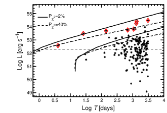
Figure 12: The log $L(T)$ distribution of Swift LGRBs with PEH data shown as red diamonds. The median value for the distribution is shown by the horizontal dashed line. To illustrate how the parameter space of the LF can be further interrogated by complementing a log $N$–log $P$ fit with the log $L$–log $T$ method we show two sets of curves: each constructed with different LF parameters but both using the same rate of 0.45 $\mathrm{Gpc}^{-3}\,\mathrm{yr}^{-1}$ (see Table 4 for parameter values). (Solid lines:) The 90% PEH bands constrain the PEH data at the MLE of 88% level(1 fail in 8); however, the corresponding log $N$–log $P$ fits for the same set of parameters produced $P_{\chi^{2}}<2\%$ (Dashed lines:) The PEH data is poorly constrained with this set of LF parameters (the MLE is 13% - 1 fail in 8); however, the corresponding log $N$–log $P$ fits produced a good fit with $P_{\chi^{2}}=40\%$.

The compatible parameter sets (in the range 0.5–0.8  $\mathrm{Gpc}^{-3}\,\mathrm{yr}^{-1}$ ) are within the range of rates estimates calculated in section 10 – however, a trend towards higher values of this range is evident. This offset is consistent with the factor of 2 discussed in section 10 and most likely results from neglecting source rate evolution within $z=0.6$ for the $V_{\mathrm{max}}$ calculation.

Rates of between 0.7 – 0.8 $\mathrm{Gpc}^{-3}\,\mathrm{yr}^{-1}$ yield both well fitting log N–log P models ($\chi^{2}/dof\sim 1.3$ and $P_{\chi^{2}}=30-33\%$) and well constrained log $L$ – log $T$ data (MLE=0.83 and $\mathcal{P}_{\mathrm{LT}}=3\%$). Within this range we take the set of parameters associated with 0.8 $\mathrm{Gpc}^{-3}\,\mathrm{yr}^{-1}$ (with the highest $P_{\chi^{2}}$ value) as the best estimate.

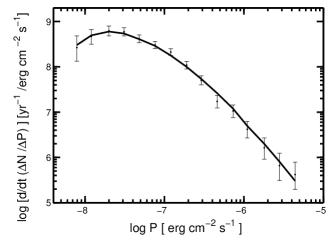
Figure 13: The log $N$ – log $P$ distribution of Swift LGRBs is fitted using using model parameters corresponding to the rate $\rho_{0}=0.8\mathrm{Gpc}^{-3}\,\mathrm{yr}^{-1}$.

Figure 13 shows the fit to the log N–log P for this best set of parameters. The values of $\rho_{0}$ we obtain are in support of recent estimates of Butler et al. (2010), Wanderman & Piran (2010) and L14. In particular, the use of the peak flux efficiency function based on the work of L14 support this study. Our results favour a steep value of $\beta$ as suggested by Butler et al. (2010) and L14.

Compatible values of $\alpha$ shown in Table 4 are in agreement with the work of Zitouni et al. (2008) who have shown that values of $-0.9<\alpha<-0.4$ are fully consistent with the prediction of an internal shock model for $\gamma$-ray emission (Rees & Meszaros, 1994). We note however that these values are slightly steeper than those obtained by L14 - this could be the result of a slight degeneracy between this parameter and $\rho_{0}$ which can both produce a vertical displacement. This suggests a LF with less free parameters could be beneficial to place additional constraints on the range of $\rho_{0}$ and will be considered in a future study.

12 conclusions

When using number count relations to probe the rate and LF dependence of LGRBs, one is confronted by a number of difficulties. Firstly, poor modeling of the complex triggering criteria of the Swift instrument can lead to large biases and poor estimates in parameters. Secondly, a complex mixing of the LF and source rate evolution can lead to degeneracies. Thirdly, for redshift dependent relations, the effect of high redshift selection biases can be difficult to quantify.

To confront the first of these obstacles we have used the results of a recent comprehensive study of the Swift instrument by L14 to produce an efficiency function for peak flux. This removes the considerable uncertainty encountered by using a single value of flux to represent the triggering sensitivity limit of the detector. An additional efficiency function has been constructed in redshift space, again based on the results of L14.

In their study, L14 determined the best range of global parameters able to reproduce the observed distribution, based on the sample of Sakamoto et al. (2011) which comprised of 414 bursts. Applying our alternative methodology to a larger sample of 644 LGRBs, our results are in good agreement.

To approach the degeneracy problem we used a suite of different methods. We have complemented more standard $V_{\mathrm{max}}$ and log $N$–log $P$ brightness distribution methods with two observation-time relations, log $(L;z)$ – log $T$. To determine initial estimates of the intrinsic (beaming uncorrected) rate density of LGRBs we have used the $V_{\mathrm{max}}$ method. To confront the small sample used in this method we have weighted the peak flux and redshift data using the corresponding efficiency functions. To verify this initial estimate we have constrained the log $z$ – log $T$ distribution.

To determine the most likely parameters of the LGRB LF we have complemented a standard log $N$–log $P$ brightness distribution with a new log $L$ – log $T$ relation. We have used both these methods simultaneously in an iterative procedure around the range of rate values calculated using $V_{\mathrm{max}}$. Our results support an event rate density at the high end of recent estimates (Butler et al., 2010; Wanderman & Piran, 2010; Cao et al., 2011b; Kanaan & de Freitas Pacheco, 2013, ,L14) and assuming a broken power law model for the LF, a steep high end slope.

There are a number of advantages in using the observation time relations. The log $L$ – log $T$ method exploits only the brightest proportion of bursts which are less likely to be below the detection threshold. We have shown that this relation is sensitive to the form of the LF, particularly the bright end. For the log $z$ – log $T$ relation, as the method is dependent on only the rarest close events, high-$z$ biases do not effect the analysis.

We have selected a broken power law LF model for this study for comparison with L14 and other recent studies that choose this form. We note that there is at present no preferred form of the LF with a number of studies choosing a power law model with an exponential cut-off (Howell & Coward, 2013; Wei et al., 2014) or log-normal distribution in luminosity (Shahmoradi, 2013). One advantage of using one of the latter forms, which have one less free parameter than a broken power model, is to minimise the risk of degeneracy in the parameter estimations. Our results suggest a small degeneracy between the rate density and the low end slope of the chosen LF. Future studies should therefore extend the work presented here and adopt a number of functional forms. A Bayesian approach would enable constraints set by the two observation time relations to be fed into the analysis as priors. Another possibility would be to investigate the form of the rate evolution, particularly the high redshift end.

To avoid added complexity, this study has not considered an evolving LF. The log $L$ – log $T$ method could be used to probe changes in different redshift intervals. A particular advantage of this method is that a log $L$ – log $T$ distribution is dependent on only the brightest proportion of data; the requirement of an adequate amount of data in each redshift interval could therefore be circumvented. An evolving LF can be modeled by modifying the break luminosity as $L_{*}(1+z)^{\delta}$ with the value of $\delta$ generally in the range 1–2. As illustrated in section 7, an increase in $L_{*}$ would produce a vertical offset in the log $L$ – log $T$ 90% PEH bands. This merits further investigation with a range of LF models and will be presented in a forthcoming study.

Appendix A The Swift LGRB data sample

Table 5: The data for the LGRB sample used in this paper. Peak energy flux data is taken from Butler’s online catalogue of Swift BAT Integrated Spectral Parameters (http://butler.lab.asu.edu/Swift/bat_spec_table.html) which is an extension of the work presented in Butler et al. (2007); Butler et al. (2010). Redshift data is taken from the Jochen Greiner online catalogue (JG) of well localized GRBs (http://www.mpe.mpg.de/~jcg/grbgen.html). Type indicates if the redshift was determined through absorbtion (A), emission (E), or photometry (P) in order of preference. Isotropic peak luminosity data is determined using the peak flux and redshift samples and corrected using the spectral parameters presented in the Butler catalogue.

GRB	$T_{obs}$	Peak Flux $\,\times 10^{-7}$	$L\,\times 10^{53}$	$z$	type	GRB	$T_{obs}$	Peak Flux $\times 10^{-7}$	$L\,\times 10^{53}$	$z$	type
	days	$(\mathrm{erg}\,\mathrm{s}^{-1}\,\mathrm{cm}^{-2})$	$(\mathrm{erg}\,\mathrm{s}^{-1})\,$				days	$(\mathrm{erg}\,\mathrm{sec}^{-1}\,\mathrm{cm}^{-2})$	$(\mathrm{erg}\,\mathrm{s}^{-1})\,$
050126	43	4.3601	6.1142	1.29	E	061110B	692	3.6977	145.96	3.44	A
050223	70	4.4748	0.3678	0.592	E	061121	703	190.31	221.53	1.31	A
050315	92	9.1043	10.799	1.95	A	061126	708	96.31	160.82	1.16	P
050318	95	23.695	5.0851	1.44	A	061222A	734	101.49	80.928	2.09	E
050319	96	7.8381	30.694	3.24	A	061222B	734	7.5264	31.051	3.36	A
050401	108	97.264	491.85	2.9	A	070103	750	9.1485	21.672	2.62	E
050505	142	13.551	153.79	4.27	A	070110	757	3.8389	2.8745	2.35	A
050525A	162	394.91	9.0548	0.606	E	070129	776	2.4624	1.8664	2.34	E
050730	227	3.3526	33.971	3.97	A	070208	785	4.2954	0.43081	1.17	E
050801	228	11.134	7.3888	1.56	P	070306	813	28.624	22.667	1.5	E
050814	241	2.668	10.104	5.3	P	070318	825	12.813	5.1693	0.836	A
050819	246	2.248	2.3008	2.5	E	070411	848	5.9716	20.434	2.95	A
050820A	247	16.84	131.13	2.61	A	070419A	856	0.63617	0.04915	0.97	A
050826	253	2.5777	0.20559	0.297	E	070419B	856	9.463	5.6712	1.96	E
050904	261	4.0053	137.06	6.29	A	070506	873	7.867	11.406	2.31	A
050908	265	4.3194	18.98	3.34	A	070521	888	61.971	82.317	1.35	P
050915A	272	8.6173	43.837	2.53	E	070529	896	6.5259	30.185	2.5	A
050922C	279	75.827	60.587	2.2	A	070611	908	4.2936	1.5831	2.04	A
051001	288	1.8412	0	0	E	070612A	909	10.263	1.315	0.617	E
051006	293	23.732	15.479	1.06	E	070721B	948	9.5099	128.46	3.63	A
051016B	303	9.0619	1.7475	0.936	E	070802	959	2.5299	5.145	2.45	A
051109A	326	32.69	53.294	2.35	A	070810A	967	9.6646	4.9436	2.17	A
051111	328	21.247	7.1898	1.55	A	071003	1020	55.702	117.12	1.6	A
051117B	334	4.7448	0.25098	0.481	E	071010A	1027	3.887	0.85028	0.98	A
060115	397	5.6315	10.369	3.53	A	071010B	1027	46.667	4.0776	0.947	A
060124	406	5.894	9.268	2.3	A	071020	1037	90.223	666.53	2.15	A
060202	414	2.1264	0.33772	0.783	E	071031	1048	1.8327	6.7129	2.69	A
060206	418	21.136	56.526	4.05	A	071117	1064	98.665	20.038	1.33	E
060210	422	19.124	163.05	3.91	A	071122	1069	1.2374	0.64926	1.14	A
060223A	435	9.1729	27.322	4.41	A	080129	1141	2.5635	43.344	4.35	A
060418	490	46.459	41.085	1.49	A	080207	1149	15.256	8.207	2.09	E
060502A	504	12.83	17.357	1.51	A	080210	1152	9.7309	24.762	2.64	A
060510B	512	2.6904	12.723	4.9	A	080310	1182	5.5655	18.748	2.42	A
060512	514	2.8502	1.6975	2.1	E	080319B	1191	482.58	654.62	0.937	A
060522	524	2.0467	8.1948	5.11	A	080319C	1191	43.143	23.703	1.95	A
060526	528	9.3424	34.828	3.22	A	080330	1202	3.6413	3.7003	1.51	A
060602A	534	2.995	1.5063	0.787	E	080411	1213	302.92	101.07	1.03	A
060604	536	2.3936	4.0413	2.14	A	080413A	1215	41.274	115.45	2.43	A
060605	537	3.038	6.6894	3.78	A	080413B	1215	129.91	14.177	1.1	A
060607A	539	10.496	16.369	3.08	A	080430	1232	17.374	2.6128	0.767	A
060707	569	5.7076	8.2473	3.42	A	080516	1248	17.045	0	0	P
060708	570	14.366	5.902	1.92	P	080520	1252	7.0829	167.94	1.54	E
060714	576	8.4294	21.027	2.71	A	080603B	1265	26.168	26.113	2.69	A
060719	581	13.721	8.7699	1.53	A	080604	1266	1.8366	1.1776	1.42	A
060729	591	7.3714	0.46839	0.54	A	080605	1267	179.1	79.228	1.64	A
060814	606	52.025	32.964	1.92	E	080607	1269	176.31	1797	3.04	A
060904B	626	14.841	0.51546	0.703	A	080707	1299	5.9124	2.8064	1.23	A
060906	628	9.7544	50.78	3.69	A	080710	1302	5.1389	3.2807	0.845	A
060908	630	27.11	12.379	1.88	A	080721	1313	188.9	2543.4	2.59	A
060912A	634	63.361	16.417	0.937	E	080804	1326	21.101	172.07	2.2	A
GRB	$T_{obs}$	Peak Flux $\,\times 10^{-7}$	$L\,\times 10^{53}$	$z$	type	GRB	$T_{obs}$	Peak Flux $\times 10^{-7}$	$L\,\times 10^{53}$	$z$	type
	days	$(\mathrm{erg}\,\mathrm{s}^{-1}\,\mathrm{cm}^{-2})$	$(\mathrm{erg}\,\mathrm{s}^{-1})\,$				days	$(\mathrm{erg}\,\mathrm{sec}^{-1}\,\mathrm{cm}^{-2})$	$(\mathrm{erg}\,\mathrm{s}^{-1})\,$
060926	648	5.8964	62.226	3.2	A	080805	1327	7.1877	7.4703	1.5	A
060927	649	21.104	97.552	5.47	A	080810	1332	11.623	101	3.35	A
061007	659	155.23	572.97	1.26	A	080905B	1357	9.3947	20.905	2.37	A
061021	673	56.262	5.1363	0.346	E	080906	1358	6.309	12.328	2.1	P
061110A	692	3.2936	0.71671	0.758	E	080913	1365	10.086	88.376	6.7	P
080916A	1368	19.385	0.70595	0.689	A	100901A	2083	3.1965	2.8301	1.41	E
080928	1380	14.11	13.439	1.69	A	100906A	2088	46.539	51.529	1.73	A
081007	1389	17.789	0.39764	0.529	A	101219B	2191	9.9342	0.55298	0.55	A
081008	1390	8.5353	4.3352	1.97	A	110106B	2213	15.383	1.2481	0.618	E
081028A	1410	2.7577	3.8604	3.04	A	110128A	2235	8.1931	60.826	2.34	A
081029	1411	1.1961	10.627	3.85	A	110205A	2242	18.762	13.645	2.22	A
081118	1430	2.3908	6.211	2.58	A	110213A	2250	66.638	40.871	1.46	A
081121	1433	76.119	82.713	2.51	A	110422A	2319	262.23	88.465	1.77	A
081203A	1445	20.13	50.856	2.05	A	110503A	2330	251.23	79.392	1.61	A
081222	1464	60.885	72.919	2.77	A	110715A	2402	452.93	23.841	0.82	A
081228	1470	10.466	45.666	3.4	P	110731A	2418	109.89	932.61	2.83	A
081230	1472	3.5155	1.5149	2	P	110801A	2418	6.0566	6.4104	1.86	A
090102	1479	47.019	80.165	1.55	A	110808A	2425	2.8731	1.8848	1.35	A
090205	1512	2.1256	7.5285	4.65	A	110818A	2435	9.8227	49.945	3.36	A
090313	1550	2.4326	10.09	3.38	A	111008A	2485	44.67	464.99	4.99	A
090417B	1584	0.83035	0.019994	0.345	E	111107A	2514	7.8189	35.944	2.89	A
090418A	1585	15.633	26.893	1.61	A	111228A	2565	69.345	7.4006	0.714	A
090423	1590	9.813	112.27	8.26	P	111229A	2566	6.9487	3.4264	1.38	A
090424	1591	537.25	11.888	0.544	A	120119A	2591	81.026	31.273	1.73	A
090426	1593	24.989	58.938	2.61	A	120326A	2658	26.094	10.186	1.8	A
090429B	1596	9.9905	147.59	9.2	P	120327A	2659	29.094	33.475	2.81	A
090516A	1613	14.017	115.26	4.11	A	120404A	2666	6.2705	18.199	2.88	A
090519	1616	3.7118	87.486	3.85	A	120712A	2764	18.292	50.36	4.17	A
090529	1626	1.8599	1.5234	2.63	A	120714B	2766	1.6976	0.012394	0.398	A
090530	1627	26.345	18.461	1.3	P	120722A	2774	9.7553	1.9846	0.959	E
090618	1645	262.75	6.3057	0.54	A	120724A	2776	1.9522	0.54163	1.48	A
090715B	1672	24.827	98.968	3	A	120729A	2781	17.904	3.6171	0.8	A
090726	1683	3.7688	4.3975	2.71	A	120802A	2785	17.174	34.619	3.8	A
090809	1696	5.6521	16.536	2.74	A	120811C	2794	22.944	22.192	2.67	A
090812	1699	31.342	158.47	2.45	A	120815A	2798	14.508	62.77	2.36	A
090814A	1701	2.4645	0.074828	0.696	A	120907A	2821	25.85	7.7046	0.97	A
090926B	1743	19.793	2.417	1.24	A	120922A	2833	9.4884	0	0	P
090927	1744	17.167	9.5402	1.37	A	121024A	2864	14.547	54.525	2.3	A
091018	1765	53.127	6.0966	0.971	A	121128A	2899	89.95	53.333	2.2	A
091020	1767	30.443	11.581	1.71	A	121201A	2902	5.4684	22.953	3.38	A
091024	1771	16.944	17.669	1.09	A	121211A	2913	4.5872	1.1832	1.02	A
091029	1776	10.697	12.401	2.75	A	121229A	2931	1.2273	3.07	2.71	A
091109A	1786	8.5831	76.505	3.08	A	130131B	2962	15.375	93.937	2.54	E
091127	1804	375.48	14.929	0.49	E	130215A	2976	12.316	1.1957	0.597	A
091208B	1815	132.43	13.99	1.06	A	130408A	3029	95.099	274.31	3.76	A
100219A	1891	2.9994	42.685	4.67	A	130418A	3039	1.4654	0.17435	1.22	A
100302A	1904	2.1454	22.19	4.81	A	130420A	3041	17.751	3.5178	1.3	A
100316B	1918	7.237	3.1676	1.18	A	130427A	3048	2986	55.576	0.34	A
100418A	1950	4.9611	0.3468	0.624	A	130427B	3048	22.982	78.77	2.78	A
100425A	1957	4.7339	1.7868	1.75	A	130505A	3056	189.29	3029.1	2.27	A
100513A	1975	2.9867	29.833	4.77	A	130511A	3060	20.399	15.428	1.3	A
100621A	2013	77.33	1.9036	0.542	E	130514A	3063	15.997	37.403	3.6	P
100724A	2046	13.849	1.7775	1.29	A	130606A	3085	18.546	309.19	5.91	A
100728B	2050	24.41	43.74	2.11	A	130612A	3091	8.3886	3.2176	2.01	A
100814A	2066	14.81	3.6671	1.44	A
100816A	2068	100.15	5.5693	0.805	A

References

- Band (2003) Band D., 2003, ApJ, 588, 945
- Band et al. (1993) Band D., et al., 1993, ApJ., 413, 281
- Bromberg et al. (2012) Bromberg O., Nakar E., Piran T., Sari R., 2012, ApJ, 749, 110
- Butler et al. (2010) Butler N. R., Bloom J. S., Poznanski D., 2010, ApJ, 711, 495
- Butler et al. (2007) Butler N. R., Kocevski D., Bloom J. S., Curtis J. L., 2007, ApJ, 671, 656
- Campisi et al. (2010) Campisi M. A., Li L.-X., Jakobsson P., 2010, MNRAS, 407, 1972
- Cao et al. (2011a) Cao X.-F., Yu Y.-W., Cheng K. S., Zheng X.-P., 2011a, MNRAS, 416, 2174
- Cao et al. (2011b) Cao X.-F., Yu Y.-W., Cheng K. S., Zheng X.-P., 2011b, MNRAS, 416, 2174
- Carroll et al. (1992) Carroll S. M., Press W. H., Turner E. L., 1992, ARAA, 30, 499
- Cobb et al. (2006) Cobb B. E., et al., 2006, ApJ, 645, L113
- Coward (2007) Coward D., 2007, New. A. Rev., 51, 539
- Coward et al. (2013) Coward D., Howell E., Branchesi M., Gendre B., Stratta G., 2013, preprint: astro-ph/1305.3366
- Coward (2005) Coward D. M., 2005, MNRAS, 360, L77
- Coward & Burman (2005) Coward D. M., Burman R. R., 2005, MNRAS, 361, 362
- Coward et al. (2008) Coward D. M., Guetta D., Burman R. R., Imerito A., 2008, MNRAS, 386, 111
- Coward et al. (2013) Coward D. M., Howell E. J., Branchesi M., Stratta G., Guetta D., Gendre B., Macpherson D., 2013, MNRAS, 432, 2141
- Coward et al. (2012) Coward D. M., Howell E. J., Piran T., Stratta G., Branchesi M., Bromberg O., Gendre B., Burman R. R., Guetta D., 2012, MNRAS, 425, 2668
- Coward et al. (2005) Coward D. M., Lilley M., Howell E. J., Burman R. R., Blair D. G., 2005, MNRAS, 364, 807
- Cucchiara et al. (2011) Cucchiara A., et al., 2011, ApJ, 736, 7
- Daigne & Mochkovitch (2007) Daigne F., Mochkovitch R., 2007, A&A, 465, 1
- Elliott et al. (2012) Elliott J., Greiner J., Khochfar S., Schady P., Johnson J. L., Rau A., 2012, A&A, 539, A113
- Epstein & Lomnitz (1966) Epstein B., Lomnitz C., 1966, Nature, p. 954–956
- Fasano & Franceschini (1987) Fasano G., Franceschini A., 1987, MNRAS, 225, 155
- Fiore et al. (2007) Fiore F., Guetta D., Piranomonte S., D’Elia V., Antonelli L. A., 2007, A&A, 470, 515
- Firmani et al. (2004) Firmani C., Avila-Reese V., Ghisellini G., Tutukov A. V., 2004, ApJ, 611, 1033
- Gehrels (1986) Gehrels N., 1986, ApJ, 303, 336
- Gehrels et al. (2004) Gehrels N., et al., 2004, ApJ, 611, 1005
- Gendre et al. (2013) Gendre B., Stratta G., Atteia J. L., Basa S., Boër M., Coward D. M., Cutini S., D’Elia V., Howell E. J., Klotz A., Piro L., 2013, ApJ, 766, 30
- Greiner et al. (2009) Greiner J., et al., 2009, ApJ, 693, 1610
- Guetta & Della Valle (2007) Guetta D., Della Valle M., 2007, ApJL, 657, L73
- Guetta & Piran (2007) Guetta D., Piran T., 2007, JCAP, 7, 3
- Guetta et al. (2005) Guetta D., Piran T., Waxman E., 2005, ApJ, 619, 412
- Hjorth et al. (2012) Hjorth J., et al., 2012, ApJ, 756, 187
- Horack et al. (1994) Horack J., Emslie A., Meegan C., 1994, ApJ, 426, L5
- Horváth et al. (2010) Horváth I., Bagoly Z., Balázs L. G., de Ugarte Postigo A., Veres P., Mészáros A., 2010, ApJ, 713, 552
- Howell et al. (2007a) Howell E., Coward D., Burman R., Blair D., 2007a, MNRAS, 377, 719
- Howell et al. (2007b) Howell E., Coward D., Burman R., Blair D., 2007b, ApJ, 666, L65
- Howell & Coward (2013) Howell E. J., Coward D. M., 2013, MNRAS, 428, 167
- Imerito et al. (2008) Imerito A., Coward D., Burman R., Blair D., 2008, MNRAS, 391, 405
- Johnson et al. (1993) Johnson N. L., Kotz S., Kemp A. W., 1993, Univariate Discrete Distributions. Hoboken, NJ: Wiley-Interscience
- Kanaan & de Freitas Pacheco (2013) Kanaan C., de Freitas Pacheco J. A., 2013, A&A, 559, A64
- Kistler et al. (2008) Kistler M. D., Yüksel H., Beacom J. F., Stanek K. Z., 2008, ApJL, 673, L119
- Kistler et al. (2013) Kistler M. D., Yuksel H., Hopkins A. M., 2013, ArXiv e-prints
- Kommers et al. (2000) Kommers J. M., Lewin W. H. G., Kouveliotou C., van Paradijs J., Pendleton G. N., Meegan C. A., Fishman G. J., 2000, ApJ, 533, 696
- Kouveliotou et al. (1993) Kouveliotou C., et al., 1993, ApJ, 413, L101
- Le & Dermer (2007) Le T., Dermer C. D., 2007, ApJ, 661, 394
- Levan et al. (2013) Levan A. J., et al., 2013, preprint: astro-ph/1307.5338
- Levan et al. (2014) Levan A. J., et al., 2014, ApJ, 781, 13
- Lien et al. (2014) Lien A., Sakamoto T., Gehrels N., Palmer D. M., Barthelmy S. D., Graziani C., Cannizzo J. K., 2014, ApJ, 783, 24
- Lu et al. (2012) Lu R.-J., Wei J.-J., Qin S.-F., Liang E.-W., 2012, ApJ, 745, 168
- Meszaros & Meszaros (1996) Meszaros A., Meszaros P., 1996, ApJ, 466, 29
- Meszaros & Meszaros (1995) Meszaros P., Meszaros A., 1995, ApJ, 449, 9
- Norris et al. (2011) Norris J. P., Gehrels N., Scargle J. D., 2011, ApJ, 735, 23
- Peacock (1983) Peacock J. A., 1983, MNRAS, 202, 615
- Perley et al. (2014) Perley D. A., et al., 2014, ApJ, 781, 37
- Planck Collaboration et al. (2013) Planck Collaboration et al., 2013, preprint: astro-ph/1303.5076)
- Porciani & Madau (2000) Porciani C., Madau P., 2000, ApJ, 548, 522
- Qin et al. (2010) Qin S.-F., Liang E.-W., Lu R.-J., Wei J.-Y., Zhang S.-N., 2010, MNRAS, 406, 558
- Rees & Meszaros (1994) Rees M. J., Meszaros P., 1994, ApJL, 430, L93
- Reichart & Meszaros (1997) Reichart D. E., Meszaros P., 1997, ApJ, 483, 597
- Sakamoto et al. (2011) Sakamoto T., Barthelmy S. D., Baumgartner W. H., Cummings J. R., Fenimore E. E., Gehrels N., Krimm H. A., Markwardt C. B., Palmer D. M., Parsons A. M., Sato G., Stamatikos M., Tueller J., Ukwatta T. N., Zhang B., 2011, ApJS, 195, 2
- Salvaterra & Chincarini (2007) Salvaterra R., Chincarini G., 2007, ApJL, 656, L49
- Salvaterra et al. (2012) Salvaterra R., et al., 2012, ApJ, 749, 68
- Salvaterra et al. (2009) Salvaterra R., Guidorzi C., Campana S., Chincarini G., Tagliaferri G., 2009, MNRAS, 396, 299
- Sethi & Bhargavi (2001) Sethi S., Bhargavi S. G., 2001, A&A, 376, 10
- Shahmoradi (2013) Shahmoradi A., 2013, ApJ, 766, 111
- Shahmoradi & Nemiroff (2011) Shahmoradi A., Nemiroff R. J., 2011, MNRAS, 411, 1843
- Stratta et al. (2013) Stratta G., Gendre B., Atteia J. L., Boër M., Coward D. M., De Pasquale M., Howell E., Klotz A., Oates S., Piro L., 2013, ApJ, 779, 66
- Virgilii et al. (2008) Virgilii F. J., Liang E.-W., Zhang B., 2008, MNRAS, 392, 91
- Wall et al. (2003) Wall J. V., Jenkins C. R., Ellis R., Huchra J., Kahn S., Rieke G., Stetson P. B., 2003, Practical Statistics for Astronomers. Cambridge University Press
- Wanderman & Piran (2010) Wanderman D., Piran T., 2010, MNRAS, 406, 1944
- Wei et al. (2014) Wei J.-J., Wu X.-F., Melia F., Wei D.-M., Feng L.-L., 2014, MNRAS, 439, 3329
- Zhang (2011) Zhang B., 2011, Comptes Rendus Physique, 12, 206
- Zitouni et al. (2008) Zitouni H., Daigne F., Mochkovich R., Zerguini T. H., 2008, MNRAS, 386, 1597