Acceleration in de Sitter spacetimes

Abstract

We propose a definition of uniform accelerated frames in de Sitter spacetimes applying the Nachtmann method of introducing coordinates using suitable point-dependent isometries. In order to recover the well-known Rindler approach in the flat limit, we require the transformation between the static frame and the accelerated one to depend continuously on acceleration, obtaining thus the natural generalization of the Rindler transformation to the de Sitter spacetimes of any dimensions.

Pacs: 04.20.Cv, 04.62.+v

Keywords: Rindler; de Sitter; accelerated frame.

1 Introduction

The problem of accelerated motions in de Sitter expanding universes is of a special interest for understanding the effects of acceleration in the presence of the natural expansion. A general method in investigating these effects relies on conformal transformations among different metrics. Thus in Ref. [1] the metrics of the static and accelerated de Sitter frames are related by a conformal scaling depending on acceleration. Another possibility is to consider some special frames of the de Sitter and Minkowki spacetimes whose metrics are conformal with the metric of the Einstein universe [2, 3, 4]. In this manner one can exploit the conformal invariance of the field equations obtaining important results concerning the scalar or electromagnetic radiation produced by the accelerated scalar or electric charges in de Sitter spacetimes.

In the present Letter we would like to propose a different approach trying to construct a natural generalization of the Rindler transformations to the de Sitter spacetime. The Rindler theory of uniform accelerated frames in Minkowski spacetime [5, 6] is the geometric framework in which the Unruh effect was introduced and then intensively studied [7, 8, 9, 10, 11, 12, 13, 14]. In other respects, the Rindler metric can be formally related to a chart of the de Sitter manifold [9, 15] whose metric is a conformal Rindler one. We may ask if could we interpret this chart as being of an accelerated observer in the de Sitter spacetime or as a mere mathematical coincidence. Our aim is to solve this problem showing that by generalising the Rindler transformation to the de Sitter geometry we obtain a new specific metric of the (uniform) accelerated frames on this manifold.

In the two-dimensional Minkowski spacetime the Rindler transformation is defined up to a space translation since the translations are Abelian isometries of this space. However, if we intend to generalize the Rindler approach to de Sitter spacetimes, we must take into account that there the space translations are not commuting with the time ones [16]. For this reason, we start with fixed initial conditions restricting ourselves to the continuous transformations with respect to the acceleration $a$, in $a=0$. Therefore, the coordinates of the static frame $\{T,X\}$ and those of the accelerated one $\{t,x\}$ (with $x\in{\mathbb{R}}$ and $t\in{\mathbb{R}}^{+}$) have to transform as

$$T = \frac{e^{ax}}{a}\sinh(at)\,,$$ (1)

$$X = \frac{e^{ax}}{a}\cosh(at)-\frac{1}{a}\,,$$ (2)

since then the limits $T\to t$ and $X\to x$ for $a\to 0$ guarantee the continuity in $a=0$. The accelerated frame, along the positive $x$ axis ($a>0$), covers the right-hand Rindler wedge where $X\in[-a^{-1},\infty)$, while for $a<0$ the left-hand wedge is its symmetric with respect to $X=0$. We note that, in this chart, the Rindler metric is independent of translations taking the well-known form [9],

$$ds^{2}=dT^{2}-dX^{2}=e^{2ax}(dt^{2}-dx^{2})\,,$$ (3)

which behaves continuously in $a=0$. In what follows, we restrict ourselves to study only the case of positive accelerations in the right-hand wedge.

We must specify that the translation introduced in Eq. (2), for assuring the continuity in $a=0$, determines the identity $i\partial_{t}=i\partial_{T}+ai(T\partial_{X}+X\partial_{T})$ that in a self-explanatory notation can be written in terms of quantum observables as $H_{acc}=H+aK$, where $H$ is the energy operator and $K$ the Lorentz generator of the static frame. However, in the case of the symmetric Rindler transformation [9] which is singular in $a=0$ (without translating $X$ with $-a^{-1}$) this identity reduces to $H_{acc}=aK$. Recently we found a metric of a mobile frame in de Sitter spacetime whose energy operator is just $aK$, but this model seems to not have a satisfactory physical meaning [17]. This is another argument for considering here the continuous Rindler transformations (1) and (2).

Our principal purpose is to generalize this conjuncture to the de Sitter manifolds requiring the transformation between the static and accelerated frames (I) to be continuous in $a=0$ and (II) to recover the above Rindler transformation in the flat limit. We first present our proposal in the simpler case of two-dimensional de Sitter manifolds, following thereafter to generalize it to the de Sitter manifolds with arbitrary dimensions.

The method we use here was proposed by Nachtmann for constructing covariant representations of the fields defined on the de Sitter spacetime, seen as a homogeneous space of its own isometry group [18]. The idea is to apply the Wigner method of orbital analysis, but in configurations instead of the momentum representation. In this manner various systems of coordinates can be introduced by choosing suitable point-dependent isometry transformations which are called here boosts [19].

The paper is organized as follows. In the second section we present the method of boosting coordinates on de Sitter manifolds, pointing out how the canonical 1-forms and the components of the Killing vector fields can be derived in any de Sitter chart. We first give the boost of the de Sitter-Painlevé chart [20, 21, 22] which is considered here the frame of the static (or fixed) observer. In the next section we postulate the form of the boosts of (uniform) accelerated frames in two dimensions and deduce the Rindler-type transformation between these frames, showing that this complies with our requirements (I) and (II). Moreover, investigating other properties, we find that the event horizon of the accelerated frame is pushed forward in the acceleration direction while the time-like Killing vector fields accomplish the same transformation rule as the one we met in the flat case mentioned above. All these results are generalised to an arbitrary number of dimensions in the fourth section. Finally, we briefly present our concluding remarks.

2 Boosting de Sitter frames

Let $(M_{d},g)$ be the $d$-dimensional de Sitter spacetime defined as the hyperboloid of radius $1/\omega$ in the $(d+1)$-dimensional flat spacetime $(\hat{M}_{d+1},\hat{\eta})$ of coordinates $z^{A}$ (labelled by the indices $A,\,B,...=0,1,2,...d$) and metric

$$\hat{\eta}={\rm diag}(1,\,\underbrace{-1,-1,...-1,-1}_{d})\,,$$ (4)

which rises or lowers these indices. Any local chart $\{x\}=\{t,\vec{x}\}$ of coordinates $x^{\mu}$ ($\mu,\nu,...=0,1,2,...d-1$) can be introduced on $(M_{d},g)$ giving a set of functions $z^{A}(x)$ which solve the hyperboloid equation,

$$\hat{\eta}_{AB}z^{A}(x)z^{B}(x)=-\frac{1}{\omega^{2}}\,.$$ (5)

Notice that here we use the vector notation for the $(d-1)$-dimensional vectors $\vec{v}=(v^{1},v^{2}...v^{d-1})$ of components $v^{i}$ ($i,j,k,...=1,2,...d-1$).

The group $\hat{G}=SO(1,d)$ is simultaneously the orthogonal group of the metric $\hat{\eta}$ and the isometry group of $(M_{d},g)$ since its transformations $z^{A}\to{\mathfrak{g}}^{A\,\cdot}_{\cdot\,B}\,z^{B}$ (or simply $z\to{\mathfrak{g}}z$) leave the equation (5) invariant for any ${\mathfrak{g}}\in\hat{G}$. In what follows we adopt the parametrization [19],

$${\mathfrak{g}}(\xi)=\exp\left(-\frac{i}{2}\,\xi^{AB}\sigma_{AB}\right)\in SO(1,d)$$ (6)

with skew-symmetric parameters, $\xi^{AB}=-\xi^{BA}$, and the covariant matrix-generators $\sigma_{AB}$ of the fundamental representation of the $so(1,d)$ algebra carried by $(\hat{M}_{d+1},\hat{\eta})$. These have the matrix elements,

$$(\sigma_{AB})^{C\,\cdot}_{\cdot\,D}=i\left(\delta^{C}_{A}\,\eta_{BD}-\delta^{C}_{B}\,\eta_{AD}\right)\,.$$ (7)

The principal $so(1,d)$ generators with physical meaning [16] are the energy $\hat{h}=\omega\sigma_{0d}$, angular momentum $\hat{j}_{kl}=\sigma_{kl}$ ($i,j,k,...=1,2...d-1$), Lorentz boosts $\hat{k}_{i}=\sigma_{0i}$, and the Runge-Lenz-type vector $\hat{r}_{i}=\sigma_{id}$. In addition, it is convenient to introduce the momentum $\hat{p}_{i}=-\omega(\hat{r}_{i}+\hat{k}_{i})$ and its dual $\hat{q}_{i}=\omega(\hat{r}_{i}-\hat{k}_{i})$ which are nilpotent matrices generating two Abelian $(d-1)$-dimensional subalgebras, $tr_{P}$ and respectively $tr_{Q}$. The matrices $\hat{p}^{i}\in tr_{P}$ generate the space translations on $(M_{d},g)$. All these generators may form different bases of the algebra $so(1,d)$ as, for example, the basis $\{\hat{h},\hat{p}_{i},\hat{q}_{i},\hat{j}_{il}\}$ or $\{\hat{h},\hat{p}_{i},\hat{j}_{il},\hat{k}_{i}\}$ [16]. We note that the $(d-1)$-dimensional restriction, $\{j_{il},k_{i}\}$, of the $so(1,d-1)$ subalgebra generate the vector representation of the group $SO(1,d-1)$.

Using the parametrization (6) we can write down the $SO(1,d)$ isometries $x\to x^{\prime}=\phi_{{\mathfrak{g}}}(x)$ according to the rule

$$z[\phi_{\mathfrak{g}}(x)]={\mathfrak{g}}\,z(x).$$ (8)

For example, the transformations ${\mathfrak{g}}\in SO(d)\subset SO(1,d)$ generated by $\hat{j}_{kl}$, are generalized $SO(d-1)$ rotations in the space of the space-like vectors $\vec{z}$. In particular, the transformations we need here are: the time translations generated by $\hat{h}$, as

$${\mathfrak{g}}_{h}(\alpha)\equiv e^{i\frac{\alpha}{\omega}\hat{h}}=\left(\begin{array}[]{cccc}\cosh\alpha&0&\cdots&\sinh\alpha\\ 0&1&\cdots&0\\ \vdots&\vdots&{\bf 1}&\vdots\\ \sinh\alpha&0&\cdots&\cosh\alpha\end{array}\right)\,,$$ (9)

the space translations,

$${\mathfrak{g}}_{p}(\vec{x})\equiv e^{-i{x}^{i}\hat{p}_{i}}=$$

$$\left(\begin{array}[]{cccc}1+\frac{1}{2}\omega^{2}\vec{x}^{2}&\omega x^{1}&\cdots&\frac{1}{2}\omega^{2}\vec{x}^{2}\\ \omega x^{1}&1&\cdots&\omega x^{1}\\ \vdots&\vdots&{\bf 1}&\vdots\\ -\frac{1}{2}\omega^{2}\vec{x}^{2}&-\omega x^{1}&\cdots&1-\frac{1}{2}\omega^{2}\vec{x}^{2}\end{array}\right)\,,$$ (14)

and the particular rotations in the plane $(z^{d-1},z^{d})$,

$${\mathfrak{g}}_{r}(\theta)\equiv e^{i\theta\hat{r}_{d-1}}=\left(\begin{array}[]{cccc}1&\cdots&0&0\\ \vdots&{\bf 1}&\vdots&\vdots\\ 0&\cdots&\cos\theta&\sin\theta\\ 0&\cdots&-\sin\theta&\cos\theta\end{array}\right),$$ (15)

generated by the matrix $\hat{r}_{d-1}$.

Such transformations can be used for introducing various types of coordinates [18, 19] since the de Sitter manifold is isomorphic to the space of left cosets $\hat{G}/G$. Indeed, if one fixes the point $z_{o}=(0,0,...0,0,\omega^{-1})^{T}\in(\hat{M}_{d+1},\hat{\eta})$, then the whole de Sitter manifold is the orbit $(M_{d},g)=\{{\mathfrak{g}}z_{o}|{\mathfrak{g}}\in\hat{G}/G\}\subset(\hat{M}_{d+1},\hat{\eta})$ where the subgroup $G=SO(1,d-1)$ is the stable group of $z_{o}$ (i. e. ${\mathfrak{g}}\,z_{o}=z_{o}\,,\,\forall{\mathfrak{g}}\in G$). Then any point $z(x)\in(M_{d},g)$ can be reached applying a point-dependent boost ${\mathfrak{b}}(x):\,z_{o}\to z(x)={\mathfrak{b}}(x)z_{o}$ which defines the functions $z^{A}(x)$ of the local coordinates $x$. In fact, these boosts are sections in the principal fiber bundle on $(M_{d},g)\sim\hat{G}/G$ whose fiber is just the isometry group $\hat{G}$.

This formalism allows one to derive the canonical $(d+1)$-dimensional 1-forms $\hat{\omega}(x)={\mathfrak{b}}^{-1}(x)d\,{\mathfrak{b}}(x)\,z_{o}$ whose components

$$\hat{\omega}^{\hat{\alpha}}(x)=\hat{e}^{\hat{\alpha}}_{\mu}(x)dx^{\mu}\,,\quad\hat{\omega}^{d}(x)=0\,,$$ (16)

give the canonical gauge fields (i. e. tetrads or vierbeins in the case of $d=4$) $\hat{e}^{\hat{\mu}}$ of the local co-frames associated to the fields $e_{\hat{\mu}}$ of the orthogonal local frames [18]. These fields are labelled by the local indices $\hat{\alpha},\hat{\mu},...$ having the same range as the natural ones. Then, the de Sitter line element of the chart $\{x\}$ can be written as

$$ds^{2}=\hat{\eta}_{AB}\hat{\omega}^{A}\,\hat{\omega}^{B}=\eta_{\hat{\alpha}\hat{\beta}}\hat{e}^{\hat{\alpha}}_{\mu}\hat{e}^{\hat{\beta}}_{\nu}dx^{\mu}dx^{\nu}=g_{\mu\nu}dx^{\mu}dx^{\nu}\,,$$ (17)

where $\eta={\rm diag}(1,-1,...-1)$ denotes the $d$-dimensional Minkowski metric.

In general, the boosts are defined up to an arbitrary gauge, ${\mathfrak{b}}(x)\to{\mathfrak{b}}(x)\lambda^{-1}(x)$, $\lambda(x)\in G$, that does not affect the functions $z^{A}(x)$ but changes the gauge fields transforming the 1-forms as $\hat{\omega}(x)\to\lambda(x)\,\hat{\omega}(x)$ [18, 19]. For this reason, $G$ is called the gauge group of $(M_{d},g)$ associated to the metric $\eta$ of the pseudo-Euclidean model of this manifold. The gauge group $G$ is important since its representations induce the covariant representations of the isometry group $\hat{G}$ [18, 16, 19].

In other respects, it is known that starting with the functions $z^{A}(x)$ one can derive the components of the Killing vector fields associated to the parameters $\xi^{AB}$. This means that we may express these components in terms of matrix elements of boost transformations. Indeed, according to our previous results [19, 16], we find that these are $k_{(AB)}^{\mu}=g^{\mu\nu}\hat{\eta}_{AC}\hat{\eta}_{BD}k^{(CD)}_{\nu}$ where the components

$$k^{(AB)}_{\mu}(x)=\frac{1}{\omega^{2}}\left[{\mathfrak{b}}^{A\,\cdot}_{\,\cdot\,d}(x)\stackrel{{\scriptstyle\leftrightarrow}}{{\partial}}_{\mu}{\mathfrak{b}}^{B\,\cdot}_{\,\cdot\,d}(x)\right]$$ (18)

are written with the notation $f\stackrel{{\scriptstyle\leftrightarrow}}{{\partial}}_{\mu}g=f\partial_{\mu}g-g\partial_{\mu}f$.

Hence we see that by choosing suitable boosts we may introduce various types of coordinates determining simultaneously the gauge fields as well as the Killing vector fields. For example, the FLRW chart $\{t,\vec{x}\}$ of the expanding portion of $(M_{d},g)$ is boosted by ${\mathfrak{b}}_{FLRW}(x)={\mathfrak{g}}_{p}(\vec{x}){\mathfrak{g}}_{h}(\omega t)$ which gives the well-known 1-forms and the FLRW metric [18]. If we change the positions of ${\mathfrak{g}}_{p}$ and ${\mathfrak{g}}_{h}$ between themselves, then we obtain the boost ${\mathfrak{b}}_{dSP}(x)={\mathfrak{g}}_{h}(\omega t){\mathfrak{g}}_{p}(\vec{x})$ of the de Sitter-Painlevé chart $\{t,\vec{x}\}$ covering the same portion. Then the canonical 1-forms,

$$\hat{\omega}^{0} = dt\,,$$

$$\hat{\omega}^{i} = dx^{i}-\omega x^{i}dt\,,$$ (19)

$$\hat{\omega}^{d} = 0\,,$$

give the de Sitter-Painlevé metric

$$ds^{2}=(1-\omega^{2}\vec{x}^{2})dt^{2}+2\omega\vec{x}\cdot d{\vec{x}}dt-d\vec{x}\cdot d\vec{x}\,,$$ (20)

which shows that the event horizon of an observer staying at rest in $\vec{x}=0$ is the sphere $S^{d-2}$ of radius $|\vec{x}|=\omega^{-1}$ as in Fig. 1.

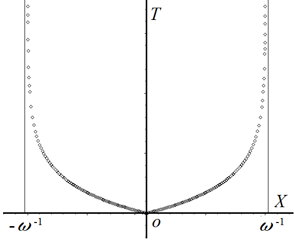
Figure 1: The null cone and the event horizons of an observer staying at $X=0$ in the frame with de Sitter-Painlevé coordinates $T,\,X$

In this chart, the Killing vector fields ${\cal K}_{(AB)}=k_{(AB)}^{\mu}\partial_{\mu}$ that may have time-like domains [23, 24] are

$${\cal K}_{(0d)}=-\frac{1}{\omega}\partial_{t}\,,$$ (21)

$${\cal K}_{(0i)}=$$

$$-e^{-\omega t}\left[x^{i}\partial_{0}+\left(\frac{\omega}{2}\,\vec{x}^{2}+\frac{1}{2\omega}(e^{2\omega t}-1)\right)\partial_{i}\right].$$ (22)

They are related to the generators of the natural representation carried by the space of scalar functions on $(M_{d},g)$. More specific, the energy operator, $H$, and the generator of the Lorentz-like transformations, $K$, are defined as [16]

$$H=-i\omega{\cal K}_{(0d)}\,,\quad K_{i}=-i{\cal K}_{(0i)}\,.$$ (23)

The Lie algebra of this representation is completed by the generators $J_{ij}=-i{\cal K}_{(ij)}$ of space rotations and the Runge-Lenz type ones, $R_{i}=-i{\cal K}_{(id)}$ [19, 16], which will be not used here.

3 Accelerating in two dimensions

Now we have all the elements we need for presenting our proposal concerning the accelerated frames in de Sitter manifolds. We start with the simplest two-dimensional case ($d=2$) assuming that the coordinates $\{t,x\}$ of an accelerated frame in $(M_{2},g)$ are introduced by the specific boost

$${\mathfrak{b}}_{acc}(t,x)={\mathfrak{g}}_{r}(\theta){\mathfrak{g}}_{h}(\Omega t){\mathfrak{g}}_{r}(-\theta){\mathfrak{g}}_{p}(u)\,,$$ (24)

where ${\mathfrak{g}}_{h}$, ${\mathfrak{g}}_{p}$ and ${\mathfrak{g}}_{r}$ are the restrictions to $d=2$ of the $(d+1)$-dimensional matrices defined by Eqs. (9), (14) and respectively (15). These depend on the parameters

$$\Omega = \sqrt{\omega^{2}+a^{2}}\,,$$ (25)

$$\theta = \arctan\frac{a}{\omega}\,,$$ (26)

$$u = \frac{1}{a}(e^{ax}-1)\,,$$ (27)

that determine the geometry of the accelerated frame. This boost was defined in accordance with the condition (I) obeying,

$$\lim_{a\to 0}{\mathfrak{b}}_{acc}(t,x)={\mathfrak{b}}_{dSP}(t,x)={\mathfrak{g}}_{h}(\omega t){\mathfrak{g}}_{p}(x)\,,$$ (28)

since for $a\to 0$ we have $\Omega\to\omega$, $\theta\to 0$ and $u\to x$.

The boost (24) gives rise to the following 1-forms

$$\hat{\omega}^{0} = dt\,e^{ax}\,,$$ (29)

$$\hat{\omega}^{1} = dx\,e^{ax}-\frac{\omega}{2a}(e^{2ax}-1)dt\,,$$ (30)

$$\hat{\omega}^{2} = 0\,.$$ (31)

determining the metric tensor of the accelerated chart $\{t,x\}$,

$$\!\!\!\!g(t,x)=$$

$$\!\!\!\!\left(\begin{array}[]{cc}e^{2ax}-\frac{\textstyle\omega^{2}}{\textstyle 4a^{2}}(e^{2ax}-1)^{2}&\frac{\textstyle\omega}{\textstyle 2a}e^{ax}(e^{2ax}-1)\\ \frac{\textstyle\omega}{\textstyle 2a}e^{ax}(e^{2ax}-1)&-e^{2ax}\end{array}\right)\,,$$ (34)

which is non-singular for any value of $a\in{\mathbb{R}}$ since $\det(g)=-e^{4ax}\not=0$. This metric tensor fulfils automatically the condition (I) as long as the boost (24) is set to satisfy Eq. (28). Then it is natural to obtain the de Sitter-Painlevé metric (for $d=2$) in the static limit,

$$\lim_{a\to 0}g(t,x)=\left(\begin{array}[]{cc}1-\omega^{2}x^{2}&\omega x\\ \omega x&-1\end{array}\right)\,.$$ (35)

However, the condition (II) cannot be imposed a priori in a similar manner at the level of boost building since there are no such boosts in Minkowski’s geometry. Therefore, we may feel lucky recovering in the flat limit precisely the genuine Rindler metric,

$$\lim_{a\to 0}g(t,x)=\left(\begin{array}[]{cc}e^{2ax}&0\\ 0&-e^{2ax}\end{array}\right)\,.$$ (36)

Thus we can say that the boost (24) solves our problem correctly in accordance with the requirements (I) and (II), introducing the coordinates $\{t,x\}$ of an uniform accelerated frame. We say that these are the natural coordinates of the accelerated frame assuming that the accelerated observer stays at rest in $x=0$.

It remains to derive the concrete transformation between the accelerated frame defined above and a static frame supposed to have the de Sitter-Painlevé coordinates $\{T,X\}$. Therefore, we have to solve the equations resulted from the identity ${\mathfrak{b}}_{dSP}(T,X)\,z_{o}={\mathfrak{b}}_{acc}(t,x)\,z_{o}$. The solutions,

$$T(t,x)\!\!\! = \!\!\!\frac{1}{\omega}\ln\left[\frac{1}{2}\frac{\omega^{2}}{\Omega^{2}}\left(\cosh\Omega t-1\right)\left(e^{2ax}+1\right)\right.$$ (37)

$$+\left.\frac{\omega}{\Omega}\,e^{ax}\sinh\Omega t+1\right]\,,$$

$$X(t,x)\!\!\! = \!\!\!\frac{1}{2a}\left[-\frac{\omega^{2}}{\Omega^{2}}\left(\cosh\Omega t-1\right)\right.$$ (38)

$$\left.+\frac{\omega}{\Omega}\sinh\Omega t\right]\left(e^{ax}-1\right)^{2}$$

$$+\,\frac{e^{ax}}{a\Omega^{2}}\left(a^{2}\cosh\Omega t+\omega^{2}\right)-\frac{1}{a}\,,$$

which represent the principal result of our proposal, can be seen as the Rindler-type transformation in the case of the two-dimensional de Sitter spacetimes. This satisfies the requirements (I) and (II) since $T(t,x)\to t$ and $X(t,x)\to x$ when $a\to 0$ while in the flat limit ($\omega\to 0$) we recover the genuine Rindler transformation as given by Eqs. (1) and (2). Notice that the initial condition, $T(0,x)=0$ and $X(0,x)=u$, is the same as in the flat case. Moreover, the translation with $a^{-1}$ considered here can be removed in Eq. (38) as in the genuine Rindler case of Eq. (2) [9].

On the other hand, these transformations help us to study how the conserved quantities of the static and accelerated frames are related among themselves. In terms of quantum observables we obtain the identity

$$H_{acc}=i\partial_{t}=H+aK\,,$$ (39)

where $H$ and $K$ are the operators of the static frame as defined by Eqs. (23) for $d=2$. Obviously, Eq. (39) is the same as in the flat case of the Rindler transformation continuous in $a=0$ we consider here. This fact is notable since the Minkowski and de Sitter observables denoted by $K$ have the same physical meaning, but very different structures.

In general, other coordinates can be used for different purposes. For example, we can proceed as in the Rindler case, introducing another space coordinate,

$$x_{\parallel}=\frac{e^{ax}}{a}\in{\mathbb{R}}^{+}\,,$$ (40)

which remains positive in the right-hand Rindler wedge (for $a>0$). This plays the role of a physical space coordinate since the metric tensor of the chart $\{t,x_{\parallel}\}$ has the form

$$\!\!\!\!g(t,x_{\parallel})=$$

$$\!\!\!\!\left(\begin{array}[]{cc}a^{2}{x_{\parallel}}^{2}-\frac{\textstyle\omega^{2}}{\textstyle 4a^{2}}(a^{2}{x_{\parallel}}^{2}-1)^{2}&\frac{\textstyle\omega}{\textstyle 2a}(a^{2}x_{\parallel}^{2}-1)\\ \frac{\textstyle\omega}{\textstyle 2a}(a^{2}x_{\parallel}^{2}-1)&-1\end{array}\right)\,,$$ (43)

(with $g_{11}=-1$). Notice that in this chart the metric tensor is singular in $a=0$ since $\det(g)=-a^{2}x_{\parallel}^{2}$.

When $a\not=0$ the chart $\{t,x_{\parallel}\}$ is useful for finding the equations of the ’light-cone’ (or null cone) by integrating the equation $ds^{2}=0$. Of course, we have to look only for solutions giving the worldlines passing through origin, $(0,a^{-1})$, since these are the borders of the future time-like domain of the observer at rest in $x_{\parallel\,0}=a^{-1}$. After a few manipulations, we find the following equations

$$t=\frac{1}{\omega}\left(\ln\frac{\Omega-\omega\pm a}{\Omega+\omega\mp a}-\ln\frac{\Omega-a\omega x_{\parallel}\pm a}{\Omega+a\omega x_{\parallel}\mp a}\right)\,,$$ (44)

representing two worldlines that for $t\to\infty$ converge asymptotically to the event horizons whose positions are given by

$$x_{\parallel\,\pm}=\sqrt{\frac{1}{\omega^{2}}+\frac{1}{a^{2}}}\pm\frac{1}{\omega}\,.$$ (45)

More specific, the forward horizon (along the acceleration direction) is at $x_{\parallel\,+}$ and the back one at $x_{\parallel\,-}$. The interpretation is simple in terms of physical coordinates where we can measure the distances among the horizons and observer’s position $x_{\parallel\,0}$ which satisfies the natural condition $x_{\parallel\,-}<x_{\parallel\,0}<x_{\parallel\,+}$. We find that $x_{\parallel\,0}-x_{\parallel\,-}<x_{\parallel\,+}-x_{\parallel\,0}$ which shows how the acceleration pushes forward both these horizons without modifying their relative distance $x_{\parallel\,+}-x_{\parallel\,-}=2\omega^{-1}$ as in Fig. 2. A similar result can be obtained by using directly the coordinate (27). Moreover, we observe that the natural coordinates of these horizons,

$$x_{\pm}=\frac{1}{a}\ln\left(\sqrt{1+\frac{a^{2}}{\omega^{2}}}\pm\frac{a}{\omega}\right)\,,$$ (46)

have the expected limits $x_{\pm}\to\pm\omega^{-1}$ for $a\to 0$.

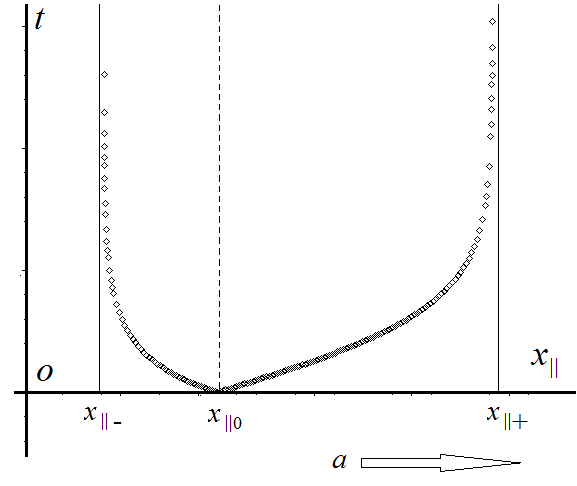
Figure 2: The null cone and the displaced horizons of an observer staying at rest in the accelerated frame at $x_{\parallel 0}=a^{-1}$.

4 Accelerating in any dimensions

The method of introducing coordinates using boosts allows us to generalize the definition of accelerated frames to any dimensions keeping the same structure of the boosts. Thus, supposing that the mobile frame of coordinates $\{t,\vec{x}\}$ is accelerated in $(M_{d},g)$ along to the axis $x^{d-1}$, we define the boosts

$${\mathfrak{b}}_{acc}(t,\vec{x})={\mathfrak{g}}_{r}(\theta){\mathfrak{g}}_{h}(\Omega t){\mathfrak{g}}_{r}(-\theta){\mathfrak{g}}_{p}(\vec{x})\,,$$ (47)

where $\vec{x}=(x^{1},x^{2},...x^{d-2},u)=(\vec{x}_{\perp},u)$ with $x^{d-1}=u$ as given by Eq. (27) and the same parameters (25) and (26). We introduce thus the chart of natural coordinates $\{t,x^{1},x^{2},...x^{d-2},x\}$ whose canonical 1-forms

$$\!\!\!\hat{\omega}^{0}=e^{ax}dt\,,$$ (48)

$$\!\!\!\hat{\omega}^{i}=dx^{i}-\omega e^{ax}x^{i}dt\,,\quad i=1,2,..,d-2\,,$$ (49)

$$\!\!\!\hat{\omega}^{d-1}=e^{ax}dx+\left[\frac{a}{2}\,\vec{x}_{\perp}^{2}-\frac{1}{2a}\left(e^{2ax}-1\right)\right]\omega dt\,,$$ (50)

$$\!\!\!\hat{\omega}^{d}=0\,,$$ (51)

generate similar properties like in the two-dimensional chart $\{t,x\}$, complying with the requirements (I) and (II). Indeed, avoiding to write the complicated form of the metric tensor in this chart, we observe that for $a\to 0$ the above 1-forms become just the de Sitter-Painlevé ones (19), while in the flat limit ($\omega\to 0$) we obtain the familiar $d$-dimensional Rindler 1-forms

$$\lim_{\omega\to 0}~{}~{}\begin{array}[]{l}\hat{\omega}^{0}\\ \hat{\omega}^{i}\\ \hat{\omega}^{d-1}\end{array}=\begin{array}[]{l}e^{ax}dt\\ dx^{i}\\ e^{ax}dx\end{array}\,.$$ (52)

The transformations between the accelerated frame and the static one cannot be studied in the general case of any $d$, but analysing some concrete examples we can draw some general conclusions. First of all we can say that these have correct flat and static limits, satisfying thus (I) and (II). Moreover, it is worth pointing out that Eq. (39) holds in any dimensions (but with $K_{d-1}$ instead of $K$). This means that, in general, for an accelerated frame in an arbitrary direction, the energy operator of the accelerated frame can be expressed in terms of static observables as $H_{acc}=H+\vec{a}\cdot\vec{K}$.

In applications it is convenient to use the chart $\{t,x^{1},x^{2},...x^{d-2},x_{\parallel}\}$ depending on the physical coordinate $x_{\parallel}$ defined by Eq. (40). Then the canonical 1-forms become,

$$\hat{\omega}^{0}=ax_{\parallel}dt\,,$$ (53)

$$\hat{\omega}^{i}=dx^{i}-a\omega x_{\parallel}x^{i}dt\,,\quad i=1,2,..,d-2\,,$$ (54)

$$\hat{\omega}^{d-1}=dx_{\parallel}-hdt\,,$$ (55)

$$\hat{\omega}^{d}=0\,,$$ (56)

where

$$h=\frac{\omega}{2a}[a^{2}(x_{\parallel}^{2}-\vec{x}_{\perp}^{2})-1]\,.$$ (57)

If we denote, in addition, $f=1-\omega^{2}\vec{x}_{\perp}^{2}$, we can write the metric tensor in a simpler form,

$$\!\!\!\!g(t,x^{1},...,x_{\parallel})=$$

$$\!\!\!\!\left(\begin{array}[]{ccccc}a^{2}x_{\parallel}^{2}f-h^{2}&\omega ax_{\parallel}x^{1}&\omega ax_{\parallel}x^{2}&\cdots&h\\ \omega ax_{\parallel}x^{1}&-1&0&\cdots&0\\ \omega ax_{\parallel}x^{2}&0&-1&\cdots&0\\ \vdots&\vdots&\vdots&&\vdots\\ h&0&0&\cdots&-1\end{array}\right)\,,$$ (63)

but which is singular in $a=0$ having $\det(g)=-a^{2}x_{\parallel}^{2}$ as in the two-dimensional case.

In this chart we can study the form of the event horizon of the accelerated observer (along to the axis $x^{d-1}$) located at $\vec{x}_{0}=(0,0,0,...a^{-1})$. Using the same method as in the two-dimensional case, we find that this remains a sphere $S^{d-2}$ of radius $\omega^{-1}$ having the center in $\vec{x}_{c}=(0,0,...,x_{\parallel\,c})$ with

$$x_{\parallel\,c}=\frac{1}{2}(x_{\parallel\,+}+x_{\parallel\,-})=\frac{\Omega}{a\omega}>\frac{1}{a}\,,$$ (64)

as it results from Eq. (45). In other words, the acceleration pushes forward the event horizon in an eccentric position but without modifying its shape.

5 Concluding remarks

We conclude that our definition of accelerated frames on de Sitter spacetimes seems to lead to a new geometric conjecture with a reasonable physical meaning. It would be interesting to compare our results with those reported so far in the literature [1, 2, 3, 4, 25].

The Nachtmann boosting method we applied here is very effective for introducing coordinates in de Sitter manifolds and pointing out geometrical properties. Therefore, we do not understand why this method is less used or quite ignored in investigating physical systems in this geometry. We hope that the examples presented here will turn people’s attention to the opportunities offered by this group theoretical approach.

Thanks to this method, we obtained accelerated charts covering the expanding portions of the de Sitter manifolds that can be interpreted as expanding universes. Similar results may be obtained on the collapsing portions by applying the antipodal transformation. We hope that our proposal presented here could be the starting point for studying the motion of classical particles or even the quantum modes in uniform accelerated frames on the de Sitter expanding or collapsing universes. A crucial topic here could be the study of the Unruh effect in this geometry.

Acknowledgments

This work was supported by a grant of the Romanian National Authority for Scientific Research. Program for research: Space Technology and Advanced Research (STAR); project number: 72/29.11.2013 of the Romanian Space Agency.

References

- [1] Podolsky J. and Griffiths J. B., Phys. Rev. D63(2000) 024006.
- [2] Bicak J. and Krtous P.,Phys. Rev. D64(2001) 124020.
- [3] Bicak J. and Krtous P., Phys. Rev. Lett.88 (2002) 211101.
- [4] Bicak J. and Krtous P., J. Math Phys.46(2005) 102504.
- [5] Born M., Ann. Phys. (Leipzig)30(1909) 1.
- [6] Rindler W., Relativity - Special, General and Cosmology (Oxford University Press, Oxford, 2006).
- [7] Unruh W. G., Phys Rev. D14(1976) 870.
- [8] Crispino, L. C. B., Higuchi A. and Matsas G. E. A., Rev. Mod. Phys80(2008) 787.
- [9] Birrel N. D. Davies P. C. W., Quantum Fields in Curved Space (Cambridge University Press, Cambridge, 1982).
- [10] DeWitt B. S., in General Relativity an Einstein Centenary Survey edited by Hawking S. W. and Israel W. (Cambridge University Press, Cambridge, 1979) 680-745
- [11] Fedotov A. M., Mur V. D., Naroszhny N. B., Belinskii V. A. and Karnakov B. M., Phys. Lett. A254(199) 126.
- [12] Takagi S., Progr. Theor. Phys. Suppl.88 (1986) 1.
- [13] Fulling S. A., Phys. Rev. D7 (1973) 2850.
- [14] Longhi P. and Soldati R., Phys. Rev. D83 (2011) 107701.
- [15] Saharian A. A. and Setare M. R., Physics LettersB584 (2004) 306.
- [16] Cotăescu I. I., GRG43 (2011) 1639.
- [17] Cotăescu I. I., arXiv:1403.3074.
- [18] Nachtmann O., Commun. Math. Phys.6 (1967) 1.
- [19] Cotăescu I. I., Mod. Phys. Lett. A28(2013) 1350033.
- [20] Gautreau R., Phys. Rev. D27 (1983) 764.
- [21] Parikh M. K., Physics LettersB546 (1969) 9691.
- [22] Pascu G., arXiv:1211.2363.
- [23] Parikh M., Samantray P. and Verlinde E., Phys.Rev. D86 (2012) 024005.
- [24] Parikh M. and Samantray P., Phys. Rev. D87 (2013) 125037.
- [25] Boblest S., Muller T. and Wunner G., Eur. J. Phys32 (2011) 1117.