Synchrotron radiation of vector bosons at relativistic colliders

Abstract

Magnetic fields produced in collisions of electrically charged particles at relativistic energies are strong enough to affect the dynamics of the strong interactions. In particular, it induces radiation of vector bosons by relativistic fermions. To develop deeper insight into this problem, I calculate the corresponding spectrum in constant magnetic field and analyze its angular distribution and mass dependence. As an application, I consider the synchrotron radiation of virtual photon by the quark-gluon plasma.

I Introduction

It has been known since the pioneering paper of Ambjorn and Olesen Ambjorn:1990jg that extremely strong electromagnetic fields are produced in high energy collisions of charged particles. In recent years it was realized that these fields have an important impact on the dynamics of the strong interactions, though their precise structure and dynamics is being debated Kharzeev:2007jp ; Tuchin:2013ie ; McLerran:2013hla ; Bzdak:2011yy ; Gursoy:2014aka ; Zakharov:2014dia . In this paper we focus on vector boson radiation by relativistic particles in an external magnetic field. In particular, I am interested in real and virtual photon production, which has important applications to the phenomenology of heavy-ion collisions Tuchin:2012mf ; Tuchin:2010gx ; Tuchin:2013bda . Synchrotron radiation of real photons in vacuum Sokolov:1968a ; Berestetsky:1982aq and in electromagnetic plasmas Baring:1988a ; Herold:1982a ; Harding:1987a has been investigated long time ago. My main goal in this paper is to calculate the synchrotron radiation of massive vector bosons and in particular virtual photons and study its mass dependence. I will assume that magnetic field is adiabatic, which is a reasonable approximation in relativistic heavy-ion collisions Tuchin:2013ie .

In order to calculate the vector meson production rate we need to know their coupling to quarks. A simple model inspired by the Vector Meson Dominance is to assume that coupling of different vector mesons to quarks has the same structure as the coupling of the photon. The corresponding terms in the Lagrangian are

$$\mathcal{L}_{\gamma}=e\bar{q}\gamma^{\mu}Qq\,A_{\mu}\,,\quad\mathcal{L}_{\rho}=g_{\rho}\bar{q}\gamma^{\mu}{\bm{\tau}}q\cdot{\bm{\rho}}_{\mu}\,,\quad\mathcal{L}_{\omega}=g_{\omega}\bar{q}\gamma^{\mu}q\,\omega_{\mu}\,,$$ (1)

where $q$ is the SU(2) doublet of $u$ and $d$ quarks, ${\bm{\tau}}$ are symmetry generators and $Q=\text{diag}(q_{u},q_{d})$. Eqs. (1) constitute a part of the quark–meson coupling model Guichon:1987jp ; Guichon:1995ue , which is used to describe the nuclear matter. Similar approach is successfully used for calculation of the vector meson production at high energy in perturbative QCD Nemchik:1996cw ; Kopeliovich:2001xj .

Throughout the paper we employ the relativistic approximation that requires fermion and the vector boson to be relativistic. Let $p=(\varepsilon,{\bm{p}})$ be the initial fermion four-momentum and $k=(\omega,{\bm{k}})$ the vector boson four-momentum, $m$ and $M$ their respective masses. Relativistic approximation requires that fermion energy before and after the vector boson emission satisfy $\varepsilon\gg m$ and $\varepsilon^{\prime}=\varepsilon-\omega\gg m$. This implies that $\varepsilon^{\prime}/\varepsilon\gg m/\varepsilon$ meaning that the vector boson does not carry away all the fermion energy. Another implication of the relativistic approximation, which is instrumental for the spectrum derivation in the next section, is that the angular distribution of the vector boson spectrum is concentrated inside a narrow solid angle with the opening angle $\theta$ around the fermion direction. This can be seen by examining the denominator of the outgoing fermion propagator

$$(p-k)^{2}-m^{2}\approx-\varepsilon\omega\left(\frac{m^{2}}{\varepsilon^{2}}+\frac{M^{2}}{\omega^{2}}\frac{\varepsilon^{\prime}}{\varepsilon}+\theta^{2}\right)\,.$$ (2)

The same expression appears in the argument of the Airy function in the formulas for the spectrum (29),(30). Thus, the radiation cone is determined by the largest among the small ratios $m/\varepsilon$ and $\sqrt{M^{2}\varepsilon^{\prime}}/\sqrt{\omega^{2}\varepsilon}<M/\omega$.

The distance between the energy levels of a fermion in magnetic field is of the order of $eB/\varepsilon$. If $eB\ll\varepsilon^{2}$ the spectrum can be considered as approximately continuous. This is always true in fields weaker than the Schwinger field $B_{S}=m^{2}/e$. In the following I will assume that the magnetic field strength is such that the quasi-classical approximation holds, i.e. $eB\ll\varepsilon^{2}$ (but not necessarily $B<B_{S}$).

The paper is structured as follows: In Sec. II.1 I derive the vector boson spectrum radiated by a fast fermion moving in a plane perpendicular to the direction of magnetic field and in Sec. II.2 I analyze its mass dependence. In Sec. III the spectrum is boosted to an arbitrary frame. Sec. III is dedicated to synchrotron radiation from plasma. Conclusions are presented in Sec. V.

II Vector boson radiation in the reaction plane ${\bm{p}}\cdot{\bm{B}}=0$.

II.1 Calculation of the spectrum

For the calculation of the vector boson spectrum I employ the method described in Baier-book ; Berestetsky:1982aq . I follow the notations of Berestetsky:1982aq apart from minor changes. The calculation is convenient to do in the frame $K_{0}$ where the fermion’s momentum is perpendicular to the direction of magnetic field. The emission probability per unit time reads Berestetsky:1982aq

$$d\dot{w}=\frac{\alpha}{(2\pi)^{2}}\frac{d^{3}k}{\omega}\int_{-\infty}^{\infty}d\tau\left\langle R^{*}_{2}R_{1}\right\rangle e^{i\Phi}\,,$$ (3)

where $\alpha=g^{2}/4\pi$ ($g$ stands for $e$, $g_{\rho}$, or $g_{\omega}$), $\left\langle R^{*}_{2}R_{1}\right\rangle$ denotes the average over the initial fermion polarization and summation over the final fermion and boson polarization and

$$\Phi =\frac{\varepsilon}{\varepsilon^{\prime}}[{\bm{k}}\cdot{\bm{r}}_{2}-{\bm{k}}\cdot{\bm{r}}_{1}-\omega\tau]+\frac{M^{2}\tau}{2\varepsilon^{\prime}}\,,$$ (4)

$$R =-\frac{\bar{u}(p^{\prime})}{\sqrt{2\varepsilon^{\prime}}}\,\gamma\cdot\epsilon^{*}\,\frac{u(p)}{\sqrt{2\varepsilon}}\,.$$ (5)

Indexes 1 and 2 is a shorthand notation meaning that the corresponding quantity is taken at time $t_{1}=t+\tau/2$ or $t_{2}=t-\tau/2$. The bi-spinor is normalized as follows:

$$u(p)=\frac{1}{\sqrt{\varepsilon+m}}\left(\begin{array}[]{c}(\varepsilon+m)\varphi_{p}\\ ({\bm{p}}\cdot{\bm{\sigma}})\varphi_{p}\end{array}\right)\,,$$ (8)

where $\varphi_{p}$ is a two-component spinor and ${\bm{\sigma}}$ are Pauli matrices. The four-momentum of the incident fermion can be written as $p=\varepsilon(1,{\bm{v}})$. Similarly, I denote

$$s=\sqrt{1-\frac{M^{2}}{\omega^{2}}}\,,$$ (9)

so that the vector boson four-momentum can be written as $k=(\omega,{\bm{k}})=\omega(1,s{\bm{n}})$, where ${\bm{n}}$ is a unit vector. Substituting (8) into (5) I obtain for transversely polarized boson

$$R_{T}=\varphi_{p^{\prime}}^{*}{\bm{\epsilon}}_{T}^{*}\cdot({\bm{A}}+i{\bm{B}}\times{\bm{\sigma}})\varphi_{p}\,,$$ (10)

where the following auxiliary vectors are introduced:

$${\bm{A}} =\left(\sqrt{\frac{\varepsilon^{\prime}+m}{\varepsilon+m}}+\sqrt{\frac{\varepsilon+m}{\varepsilon^{\prime}+m}}\right)\frac{\sqrt{\varepsilon}}{\sqrt{2\varepsilon^{\prime}}}{\bm{v}}\,,$$ (11)

$${\bm{B}} =\left[\left(\sqrt{\frac{\varepsilon^{\prime}+m}{\varepsilon+m}}-\sqrt{\frac{\varepsilon+m}{\varepsilon^{\prime}+m}}\right){\bm{p}}+\sqrt{\frac{\varepsilon+m}{\varepsilon^{\prime}+m}}\,{\bm{k}}\right]\frac{1}{2\sqrt{\varepsilon\varepsilon^{\prime}}}\,,$$ (12)

and $\varepsilon^{\prime}=\varepsilon-\omega$. Multiplying (10) by its complex conjugate and averaging using the formula $\left\langle\epsilon_{T,j}\epsilon_{T,k}\right\rangle=(\delta_{jk}-n_{j}n_{k})/2$ we get

$$\left\langle R^{*}_{T,2}R_{T,1}\right\rangle={\bm{A}}_{1}\cdot{\bm{A}}_{2}-({\bm{A}}_{1}\cdot{\bm{n}})({\bm{A}}_{2}\cdot{\bm{n}})+{\bm{B}}_{1}\cdot{\bm{B}}_{2}+({\bm{B}}_{1}\cdot{\bm{n}})({\bm{B}}_{2}\cdot{\bm{n}})\,.$$ (13)

Expanding (11),(12) in $m^{2}/\varepsilon^{2}$ and $M^{2}/\omega^{2}$ yields

$${\bm{A}}\approx\left(1+\frac{\varepsilon}{\varepsilon^{\prime}}\right)\frac{{\bm{v}}}{2}\,,$$ (14)

$${\bm{B}}\approx\frac{\omega}{2\varepsilon^{\prime}}\left(-{\bm{v}}+{\bm{n}}+\frac{m}{\varepsilon}{\bm{n}}+(s-1){\bm{n}}\right)\,.$$ (15)

Terms like ${\bm{v}}_{1}\cdot{\bm{n}}$ arising in (13) can be simplified using integration by parts in (3) as follows Berestetsky:1982aq

$${\bm{v}}_{1}\cdot{\bm{n}}\,e^{i\Phi}={\bm{v}}_{2}\cdot{\bm{n}}\,e^{i\Phi}=\left[1+\frac{\omega(s^{2}-1)}{2s\varepsilon}\right]e^{i\Phi}\,,$$ (16)

where terms proportional to the total time derivative with respect to $t_{1}$, which vanish upon integration over time in (3), are dropped. Substituting (14),(15) into (13) I derive

$$\left\langle R^{*}_{T,2}R_{T,1}\right\rangle=\frac{\varepsilon^{\prime 2}+\varepsilon^{2}}{2\varepsilon^{\prime 2}}({\bm{v}}_{1}\cdot{\bm{v}}_{2}-1)+\frac{M^{2}}{2\omega^{2}}\frac{\omega}{\varepsilon^{\prime}}\left(\frac{\varepsilon}{\varepsilon^{\prime}}+\frac{\varepsilon^{\prime}}{\varepsilon}\right)+\frac{\omega^{2}m^{2}}{2\varepsilon^{2}\varepsilon^{\prime 2}}\,.$$ (17)

Explicit expression for the fermion trajectory in a plane perpendicular to magnetic field yields at small $\tau$:

$${\bm{v}}_{1}\cdot{\bm{v}}_{2}=1-\frac{m^{2}}{\varepsilon^{2}}-\frac{1}{2}\omega_{B}^{2}\tau^{2}\,,$$ (18)

where $\omega_{B}=eB/\varepsilon$ is the synchrotron frequency. Thus, (17) takes form

$$\left\langle R^{*}_{T,2}R_{T,1}\right\rangle=-\frac{\varepsilon^{\prime 2}+\varepsilon^{2}}{2\varepsilon^{\prime 2}}\omega_{B}^{2}\tau^{2}+\frac{M^{2}}{2\omega^{2}}\frac{\omega}{\varepsilon^{\prime}}\left(\frac{\varepsilon}{\varepsilon^{\prime}}+\frac{\varepsilon^{\prime}}{\varepsilon}\right)-\frac{m^{2}}{\varepsilon\varepsilon^{\prime}}\,.$$ (19)

The longitudinal polarization is described by the four-vector $\epsilon_{L}=(s,\hat{{\bm{n}}})/\sqrt{s^{2}-1}$, which satisfies $\epsilon\cdot k=0$ and $\epsilon^{2}=1$. Writing $R=-j\cdot\epsilon$ and using the Ward identity $j\cdot k=0$ we have $j^{0}=s{\bm{j}}\cdot{\bm{n}}$ implying that

$$j\cdot\epsilon_{L}=\frac{j^{0}s-{\bm{j}}\cdot{\bm{n}}}{\sqrt{s^{2}-1}}=\sqrt{s^{2}-1}\,{\bm{j}}\cdot{\bm{n}}\,.$$ (20)

Using (8) and (5) produces

$$R_{L}=i\sqrt{1-s^{2}}\,\varphi_{p^{\prime}}^{*}(F+i{\bm{\sigma}}\cdot{\bm{G}})\varphi_{p}\,.$$ (21)

and

$$\left\langle R^{*}_{L,2}R_{L,1}\right\rangle=(1-s^{2})(F_{2}F_{1}+{\bm{G}}_{2}\cdot{\bm{G}}_{1})\,,$$ (22)

where

$$F =\frac{1}{2\sqrt{\varepsilon\varepsilon^{\prime}}\sqrt{\varepsilon+m}\sqrt{\varepsilon^{\prime}+m}}[(\varepsilon^{\prime}+m)({\bm{n}}\cdot{\bm{p}})+(\varepsilon+m)({\bm{p}}^{\prime}\cdot{\bm{n}})]$$ (23)

$${\bm{G}} =\frac{1}{2\sqrt{\varepsilon\varepsilon^{\prime}}\sqrt{\varepsilon+m}\sqrt{\varepsilon^{\prime}+m}}[(\varepsilon^{\prime}+m)({\bm{n}}\times{\bm{p}})+(\varepsilon+m)({\bm{n}}\times{\bm{p}}^{\prime})]\,,$$ (24)

with ${\bm{p}}^{\prime}={\bm{p}}-{\bm{k}}$. In view of a small factor $1-s^{2}$ in the right hand side of (22) we only need to keep terms of the order one in expansion of $F$ and ${\bm{G}}$ in powers of $m^{2}/\varepsilon^{2}$ and $M^{2}/\omega^{2}$. Thus, in view of (16) ${\bm{p}}\cdot{\bm{n}}\approx\varepsilon$, ${\bm{p}}^{\prime}\cdot{\bm{n}}\approx\varepsilon^{\prime}$ and we have $F\approx 1$, ${\bm{G}}\approx-\frac{\omega}{2\varepsilon^{\prime}}\,{\bm{n}}\times{\bm{v}}$. This implies that ${\bm{G}}_{1}\cdot{\bm{G}}_{2}\propto 1-{\bm{v}}_{1}\cdot{\bm{v}}_{2}\sim m^{2}/\varepsilon^{2}$ can be neglected and we derive

$$\left\langle R^{*}_{L,2}R_{L,1}\right\rangle\approx\frac{M^{2}}{\omega^{2}}\,.$$ (25)

The expression in the exponent of (3) upon expansion in $\tau$ and then in $M/\omega$ becomes

$$\Phi=-\frac{\varepsilon}{\varepsilon^{\prime}}\omega\tau\left[1-s{\bm{n}}\cdot{\bm{v}}+\frac{\omega}{2\varepsilon}(s^{2}-1)+s\omega_{B}^{2}\frac{\tau^{2}}{24}\right]\approx-\frac{\varepsilon}{\varepsilon^{\prime}}\omega\tau\left[1-{\bm{n}}\cdot{\bm{v}}+\frac{M^{2}}{2\omega^{2}}\frac{\varepsilon^{\prime}}{\varepsilon}+\omega_{B}^{2}\frac{\tau^{2}}{24}\right]\,.$$ (26)

Substituting (19), (25) and (26) into (3) we obtain for the transverse and longitudinal vector boson production rates

$$d\dot{w}_{T}= \frac{\alpha}{(2\pi)^{2}}\frac{d^{3}k}{\omega}\int_{-\infty}^{\infty}d\tau\exp\left\{-\frac{i\varepsilon}{\varepsilon^{\prime}}\omega\tau\left[1-{\bm{n}}\cdot{\bm{v}}+\frac{M^{2}}{2\omega^{2}}\frac{\varepsilon^{\prime}}{\varepsilon}+\omega_{B}^{2}\frac{\tau^{2}}{24}\right]\right\}$$

$$\times\,\left[-\frac{\varepsilon^{\prime 2}+\varepsilon^{2}}{4\varepsilon^{\prime 2}}\omega_{B}^{2}\tau^{2}+\frac{M^{2}}{2\omega^{2}}\frac{\omega}{\varepsilon^{\prime}}\left(\frac{\varepsilon}{\varepsilon^{\prime}}+\frac{\varepsilon^{\prime}}{\varepsilon}\right)-\frac{m^{2}}{\varepsilon\varepsilon^{\prime}}\right]\,,$$ (27)

$$d\dot{w}_{L}= \frac{\alpha}{(2\pi)^{2}}\frac{d^{3}k}{\omega}\frac{M^{2}}{\omega^{2}}\int_{-\infty}^{\infty}d\tau\exp\left\{-\frac{i\varepsilon}{\varepsilon^{\prime}}\omega\tau\left[1-{\bm{n}}\cdot{\bm{v}}+\frac{M^{2}}{2\omega^{2}}\frac{\varepsilon^{\prime}}{\varepsilon}+\omega_{B}^{2}\frac{\tau^{2}}{24}\right]\right\}\,.$$ (28)

One can do integrals over $\tau$ using equations (71) and (73) which yields the angular distribution of the spectrum

$$\frac{d\dot{w}_{T}}{d\omega d\Omega}= \frac{\alpha}{\pi}\omega\left(\frac{\varepsilon^{\prime}}{\varepsilon\omega\omega_{B}^{2}}\right)^{1/3}\left[\frac{M^{2}}{2\omega^{2}}\left(\frac{\varepsilon}{\varepsilon^{\prime}}+\frac{\varepsilon^{\prime}}{\varepsilon}\right)\frac{\varepsilon+\varepsilon^{\prime}}{\varepsilon^{\prime}}-\frac{m^{2}}{\varepsilon\varepsilon^{\prime}}+2\left(1-{\bm{n}}\cdot{\bm{v}}\right)\frac{\varepsilon^{\prime 2}+\varepsilon^{2}}{\varepsilon^{\prime 2}}\right]$$

$$\times\text{Ai}\left(2\left(\frac{\varepsilon\omega}{\varepsilon^{\prime}\omega_{B}}\right)^{2/3}\left(1-{\bm{n}}\cdot{\bm{v}}+\frac{M^{2}\varepsilon^{\prime}}{2\omega^{2}\varepsilon}\right)\right)\,,$$ (29)

$$\frac{d\dot{w}_{L}}{d\omega d\Omega}= \frac{\alpha}{\pi}\omega\left(\frac{\varepsilon^{\prime}}{\varepsilon\omega\omega_{B}^{2}}\right)^{1/3}\frac{M^{2}}{\omega^{2}}\,\text{Ai}\left(2\left(\frac{\varepsilon\omega}{\varepsilon^{\prime}\omega_{B}}\right)^{2/3}\left(1-{\bm{n}}\cdot{\bm{v}}+\frac{M^{2}\varepsilon^{\prime}}{2\omega^{2}\varepsilon}\right)\right)\,,$$ (30)

where we used $d^{3}k=s\omega^{2}d\omega d\Omega\approx\omega^{2}d\omega d\Omega$. Notice the follwing expression

$$2\left(1-{\bm{n}}\cdot{\bm{v}}+\frac{M^{2}\varepsilon^{\prime}}{2\omega^{2}\varepsilon}\right)\approx\theta^{2}+\frac{m^{2}}{\omega^{2}}+\frac{M^{2}\varepsilon^{\prime}}{2\omega^{2}\varepsilon}\,,$$ (31)

which appears in the argument of the Airy function. It is proportional to the denominator of the outgoing fermion propagator (2) and guarantees emission of vector boson into a narrow cone.

Integration over the photon directions is convenient to do in (27),(28) followed by integration over $\tau$ Berestetsky:1982aq . The result is

$$\frac{d\dot{w}_{T}}{d\omega}= -\frac{\alpha m^{2}}{\varepsilon^{2}}\left\{\left(1-\frac{M^{2}}{2\omega\varepsilon^{\prime}}\frac{\varepsilon^{2}+\varepsilon^{\prime 2}}{m^{2}}\right)\int_{z}^{\infty}\text{Ai}(z^{\prime})dz^{\prime}+\left(\frac{\varepsilon}{\varepsilon^{\prime}}\right)^{1/3}\left(\frac{\omega_{B}}{\omega}\right)^{2/3}\frac{\varepsilon^{2}+\varepsilon^{\prime 2}}{m^{2}}\text{Ai}^{\prime}(z)\right\}\,,$$ (32)

$$\frac{d\dot{w}_{L}}{d\omega}= \frac{\alpha M^{2}\varepsilon^{\prime}}{\omega^{2}\varepsilon}\int_{z}^{\infty}\text{Ai}(z^{\prime})dz^{\prime}\,,$$ (33)

where

$$z=\left(\frac{\varepsilon}{\varepsilon^{\prime}}\right)^{2/3}\left(\frac{\omega}{\omega_{B}}\right)^{2/3}\left(\frac{m^{2}}{\varepsilon^{2}}+\frac{M^{2}}{\omega^{2}}\frac{\varepsilon^{\prime}}{\varepsilon}\right)\,.$$ (34)

II.2 Analysis of the spectrum

Vector boson spectrum (32),(33) is a function of $\omega$ and $\varepsilon$. Instead, we can express the spectrum in terms of the boost-invariant dimensionless quantities $X$ and $\xi$ defined as follows:

$$X=\sqrt{-\frac{e^{2}}{m^{6}}\,(F_{\mu\nu}p^{\nu})^{2}}\approx\frac{\omega_{B}\varepsilon^{2}}{m^{3}}=\frac{eB\varepsilon}{m^{3}}$$ (35)

and

$$\xi=\frac{\omega}{\omega_{c}}\,,$$ (36)

where

$$\omega_{c}=\frac{\varepsilon X}{\frac{2}{3}+X}\,,$$ (37)

is the characteristic frequency of the classical photon spectrum. Its is also convenient to denote $\mu=M/m$. In terms of these variables we can write

$$z=\frac{\xi^{2/3}}{[\frac{2}{3}+X(1-\xi)]^{2/3}}+\mu^{2}\frac{[\frac{2}{3}+X(1-\xi)]^{1/3}(\frac{2}{3}+X)}{X^{2}\xi^{4/3}}\,\,,$$ (38)

$$\varepsilon^{\prime}=\frac{\omega_{c}\left[\frac{2}{3}+X(1-\xi)\right]}{X}\,.$$ (39)

Becasue $\varepsilon^{\prime}\geq 0$, it follows form (39) that

$$\xi\leq\frac{2}{3X}+1\,.$$ (40)

When multiplied by $\omega$, (32),(33) yield the radiation power. Dividing it by $3/2$ of the total classical photon radiation power $\alpha m^{2}X^{2}$ we represent the spectrum in terms of the dimensionless quantities

$$J_{\lambda}(\xi,X,\mu)=\frac{\omega}{\alpha m^{2}X^{2}}\frac{d\dot{w}_{\lambda}}{d\xi}\,,\quad\lambda=L,T\,.$$ (41)

Their explicit form reads as follows

$$J_{T}= -\frac{\xi}{(\frac{2}{3}+X)^{2}}\left\{\left[1-\mu^{2}\left(\frac{\frac{2}{3}+X}{\xi X}+\frac{\xi X}{\frac{4}{3}+2X(1-\xi)}\right)\right]\int_{z}^{\infty}\text{Ai}(z^{\prime})dz^{\prime}\right.$$

$$\quad\left.+\frac{(\frac{2}{3}+X)^{2}+[\frac{2}{3}+X(1-\xi)]^{2}}{\xi^{2/3}[\frac{2}{3}+X(1-\xi)]^{1/3}(\frac{2}{3}+X)}\text{Ai}^{\prime}(z)\right\}\,,$$ (42)

$$J_{L}= \frac{\mu^{2}[\frac{2}{3}+X(1-\xi)]}{X^{2}\xi(\frac{2}{3}+X)}\int_{z}^{\infty}\text{Ai}(z^{\prime})dz^{\prime}\,.$$ (43)

Airy function exponentially decays at large values of its argument, hence the spectrum is suppressed at $z\gg 1$. Variable $z$ as a function of $\xi$ has a minimum $z_{0}$ at $\xi_{0}$ that depends on the values of $X$ and $\mu$. The main contribution to the spectrum comes form the kinematic region $z<1$ which exists only if $z_{0}<1$. To determine $z_{0}$ and $\xi_{0}$ it is convenient to use instead of $\xi$ an auxiliary variable $u$:

$$u =\frac{1}{\xi}\left[\frac{2}{3}+X(1-\xi)\right]\,,$$ (44)

$$z =\frac{1}{u^{2/3}}+\frac{\mu^{2}u^{1/3}(u+X)}{X^{2}}\,.$$ (45)

The minimum of $z$ as a function of $u$ is located at

$$u_{0}=\frac{X}{8}\left(\sqrt{1+\frac{32}{\mu^{2}}}-1\right)\,.$$ (46)

The corresponding value of $\xi$ reads

$$\xi_{0}=\frac{\frac{2}{3}+X}{u_{0}+X}=\frac{\frac{2}{3}+X}{X}\frac{8}{7+\sqrt{1+\frac{32}{\mu^{2}}}}\,.$$ (47)

At $\mu\ll 1$, corresponding to an almost real photon,

$$\ u_{0}\approx\frac{X}{\sqrt{2}\mu}\,,\quad\xi_{0}\approx\mu\sqrt{2}\,\frac{\frac{2}{3}+X}{X}\,,\quad\mu\ll 1\,.$$ (48)

Replacing $X=\sqrt{2}u_{0}\mu$ in (45) we get

$$z_{0}\approx\frac{3}{2u_{0}^{2/3}}\,,\quad\mu\ll 1\,.$$ (49)

Thus, the condition $z_{0}<1$ is satisfied only if $X>2.6\mu$. Otherwise, the spectrum is exponentially suppressed.

In the opposite case, which is realized e.g. in production of high invariant mass dileptons, $\mu^{2}\gg 32$ we have

$$u_{0}\approx\frac{2X}{\mu^{2}}\,,\quad\xi_{0}\approx\frac{\frac{2}{3}+X}{X}\,,\quad\mu\gg 4\sqrt{2}\,,$$ (50)

Comparing with (40), we observe that in this case the minimum of $z$ is very close to the upper cutoff of the boson spectrum (i.e. when the boson takes nearly all energy of the fermion). Using $X=u_{0}\mu^{2}/2$ in (45) we have

$$z_{0}\approx\frac{3}{u_{0}^{2/3}}\,,\quad\mu\gg 4\sqrt{2}\,.$$ (51)

In this case $z_{0}<1$ is satisfied if $X>2.6\mu^{2}$ which is a much stronger condition than in the previous case.

The main contribution to the spectrum arises from $z\sim 1$, which for $X$ and $\mu$ satisfying the above constraints and taking (45) into account happens when $u\sim 1$ fairly independently from the value of $\mu$. This statement has been verified numerically. In particular, according to (44) $u\sim 1$ means that $\xi\sim\frac{2}{3}+X(1-\xi)$. In weak fields $X\ll 1$, $\xi\sim 1$ and so $\omega\sim\omega_{c}\sim\varepsilon X$, while in strong fields $X\gg 1$, $\xi\sim X\varepsilon^{\prime}/\omega_{c}$ (see (39)) implying that $\varepsilon^{\prime}\sim\omega/X\sim\varepsilon/X\sim m^{3}/eB$ Berestetsky:1982aq .

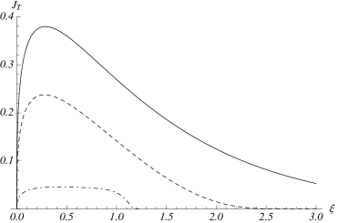
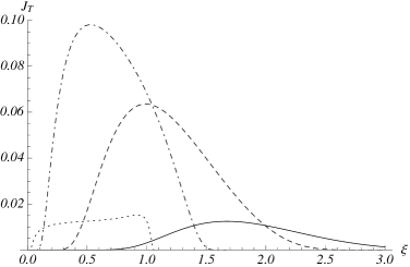
$(a)$	$(b)$
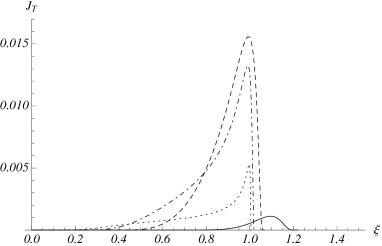
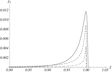
$(c)$	$(d)$

Figure 1: Spectrum of transversely polarized vector bosons $J_{T}$ as a function of $\xi$. (a) $\mu=0$ and $X=0$ (solid line), $X=0.3$ (dashed line), $X=3$ (dash-dotted line). (b) $\mu=0.3$ and $X=0.15$ (solid line), $X=0.3$ (dashed line), $X=1$ (dash-dotted line), $X=10$ (dotted lines). (c) $\mu=3$ and $X=3$ (solid line), $X=10$ (dashed line), $X=30$ (dash-dotted line), $X=100$ (dotted lines). (d) $\mu=10$ and $X=100$ (solid line), $X=400$ (dashed line), $X=1000$ (dash-dotted line). Notice different scales of the $x$ and $y$ axes.

These features of the spectrum are seen in Figs. 1–3. In Fig. 1 the transverse vector boson spectrum as a function of $\xi$ is shown at different values of $X$ and $\mu$. The longitudinal bosons are much more abundantly produced than the transverse one, which can be seen by comparing Fig. 1(b) and Fig. 2. Therefore, Fig. 1 represents approximately the total spectrum. The general trend observed in all figures is that the spectrum decreases with increase of $\mu$. At larger $\mu$ it tends to peak around $\xi=1$. This is because with increase of $\mu$, $X$ also increases, see the text after (50),(51); it follows from (50) that once $X\gg 1$, the typical $\xi$ is about 1.

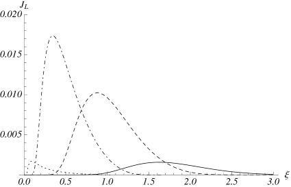
Figure 2: Spectrum of longitudinaly polarized vector bosons $J_{L}$ as a function of $\xi$ at $\mu=0.3$ and $X=0.15$ (solid line), $X=0.3$ (dashed line), $X=1$ (dash-dotted line), $X=10$ (dotted lines)

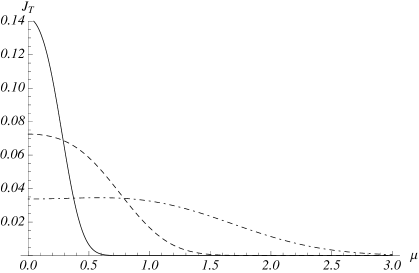
Figure 3: Spectrum of transversely polarized vector bosons $J_{T}$ as a function of $\mu$ at $\xi=1$ and $X=0.3$ (solid line), $X=1$ (dashed line) and $X=3$ (dashed-dotted line).

III Vector boson spectrum in an arbitrary frame

Consider now a reference frame $K$ where fermions have an arbitrary direction of momentum. It is convenient to change our notations. We will append a subscript 0 to all quantities pertaining to the reference frame $K_{0}$. Thus, for example, $\varepsilon_{0}$ and $\omega_{0}$ are the fermion and vector boson energies in $K_{0}$, whereas $\varepsilon$ and $\omega$ are the fermion and vector boson energies in $K$. Let the $y$-axis be in the magnetic field direction ${\bm{B}}=B\hat{{\bm{y}}}$ and ${\bm{V}}=V\hat{{\bm{y}}}$ be velocity of $K$ with respect to $K_{0}$. Then the Lorentz transformation reads

$$p_{x0}=p_{x}\,,\quad 0=p_{y0}=\gamma(p_{y}+V\varepsilon)\,,\quad p_{z0}=p_{z}\,,\quad\varepsilon_{0}=\gamma(\varepsilon+Vp_{y})\,.$$ (52)

$$k_{x0}=k_{x}\,,\quad k_{y0}=\gamma(k_{y}+V\omega)\,,\quad k_{z0}=k_{z}\,,\quad\omega_{0}=\gamma(\omega+Vk_{y})\,.$$ (53)

$${\bm{B}}_{0}={\bm{B}}\,,$$ (54)

where $\gamma=1/\sqrt{1-V^{2}}$. It follows from the second equation in (52) that

$$V=-\frac{p_{y}}{\varepsilon}$$ (55)

and

$$\varepsilon_{0}=\sqrt{\varepsilon^{2}-p_{y}^{2}}\,,\qquad\omega_{0}=\frac{\omega\varepsilon-p_{y}k_{y}}{\sqrt{\varepsilon^{2}-p_{y}^{2}}}\,.$$ (56)

Using the boost invariance of $k\cdot p$ we get

$$1-{\bm{n}}_{0}\cdot{\bm{v}}_{0}=\frac{\omega\varepsilon}{\omega_{0}\varepsilon_{0}}(1-{\bm{n}}\cdot{\bm{v}})\,,$$ (57)

accurate up to the terms of the order $m^{2}/\varepsilon^{2}$ and $M^{2}/\omega^{2}$.

Transformation of the photon emission rate reads Tuchin:2013bda

$$\frac{d\dot{w}}{d\Omega d\omega}=\frac{1}{\gamma^{2}(1+V\cos\theta)}\frac{d\dot{w}_{0}}{d\Omega_{0}d\omega_{0}}=\frac{\omega\varepsilon_{0}}{\varepsilon\omega_{0}}\frac{d\dot{w}_{0}}{d\Omega_{0}d\omega_{0}}\,,$$ (58)

where $\theta$ is angle between the photon momentum ${\bm{k}}$ and the magnetic field, i.e. $\cos\theta=n_{y}$. In the last step we used (55) and (56). $d\dot{w}_{0}$ in the right-hand-side of (58) is given by (29) and (30) with the replacements $\varepsilon\to\varepsilon_{0}$, $\omega\to\omega_{0}$ etc.

IV Vector boson radiation by a plasma

A system of electrically charged particles in thermal equilibrium in external magnetic field radiates vector bosons at the following rate per unit interval of vector boson energy $d\omega$ into a solid angle $d\Omega$:

$$\frac{dN}{dtd\Omega d\omega}=2N_{c}\sum_{f}\int\frac{d\mathcal{V}d^{3}p}{(2\pi)^{3}}f(\varepsilon)[1-f(\varepsilon^{\prime})]\frac{d\dot{w}}{d\Omega d\omega}\,,$$ (59)

where the sum runs over all charged particle species in plasma, and $f(\varepsilon)$ are their distribution functions. Integration over the fermion momentum can be done using a Cartesian reference frame span by three unit vectors ${\bm{e}}_{1},{\bm{e}}_{2},{\bm{n}}$, such that vector ${\bm{B}}$ lies in plane span by ${\bm{e}}_{1},{\bm{n}}$. In terms of the polar and azimuthal angles $\chi$ and $\psi$ we can write

$${\bm{v}}=v(\cos\chi\,{\bm{n}}+\sin\chi\cos\psi\,{\bm{e}}_{1}+\sin\chi\sin\psi\,{\bm{e}}_{2})\,,$$ (60)

$${\bm{B}}=B(\cos\theta\,{\bm{n}}_{1}+\sin\theta\,{\bm{e}}_{1})\,.$$ (61)

Element of the solid angle is $do=d\cos\chi\,d\psi$. In this reference frame

$$p_{y}=\frac{{\bm{p}}\cdot{\bm{B}}}{B}=\varepsilon v(\cos\chi\cos\theta+\sin\chi\cos\psi\sin\theta)\,,$$ (62)

$$k_{y}=\frac{{\bm{k}}\cdot{\bm{B}}}{B}=k\cos\theta\,,$$ (63)

$${\bm{n}}\cdot{\bm{v}}=v\cos\chi\,.$$ (64)

Fermions moving in plasma parallel to the magnetic field direction do not radiate due to the vanishing Lorentz force. Taking into account that at high energies fermions radiate mostly into a narrow cone with the opening angle $\chi\sim m/\varepsilon,M/\omega$ (see (2)), we conclude that vector boson radiation at angles $\theta\lesssim m/\varepsilon,M/\omega$ can be neglected. Thus, expanding at small $\chi$ we obtain from (56),(62)

$$\varepsilon_{0}\approx\varepsilon\sin\theta\,,\quad\omega_{0}\approx\omega\sin\theta\,,\qquad\theta>\frac{m}{\varepsilon},\frac{M}{\omega}\,.$$ (65)

Omission of terms of order $m/\varepsilon$, $M\omega$ is consistent with the accuracy of (29),(30). Dependence of the integrand of (59) on the fermion direction specified by the angles $\chi$, $\psi$ comes only through (57), viz.

$$1-{\bm{n}}_{0}\cdot{\bm{v}}_{0}=\frac{1}{\sin^{2}\theta}\left(1-\cos\chi+\frac{m^{2}}{2\varepsilon^{2}}\right)\,.$$ (66)

For this reason, integration over the quark momentum directions is similar to the one that led us from (27), (28) to (32), (33) (in the $K_{0}$ reference frame). Writing (59) as

$$\frac{dN}{dtd\Omega d\omega}= \frac{2N_{c}}{(2\pi)^{3}}\sum_{f}\int d\mathcal{V}\int_{\omega}^{\infty}d\varepsilon\,\varepsilon^{2}f(\varepsilon)[1-f(\varepsilon^{\prime})]\sum_{\lambda=L,T}\int do\,\frac{d\dot{w}_{\lambda}}{d\Omega d\omega}$$ (67)

and substituting (58), (27), (28) (with appropriate notation changes as described in Sec. III) and (65) we integrate first over $do$ and then over $\tau$ with the following result

$$\int do\,\frac{d\dot{w}_{T}}{d\Omega d\omega}= -\frac{\alpha m^{2}}{\varepsilon^{2}}\sin^{2}\theta\left\{\left(1-\frac{M^{2}}{2\omega\varepsilon^{\prime}}\frac{\varepsilon^{2}+\varepsilon^{\prime 2}}{m^{2}}\right)\int_{z_{\theta}}^{\infty}\text{Ai}(z^{\prime})dz^{\prime}\right.$$

$$\left.+(\sin\theta)^{2/3}\left(\frac{\varepsilon}{\varepsilon^{\prime}}\right)^{1/3}\left(\frac{\omega_{B}}{\omega}\right)^{2/3}\frac{\varepsilon^{2}+\varepsilon^{\prime 2}}{m^{2}}\text{Ai}^{\prime}(z_{\theta})\right\}\,,$$ (68)

$$\int do\,\frac{d\dot{w}_{L}}{d\Omega d\omega}= \frac{\alpha M^{2}\varepsilon^{\prime}}{\omega^{2}\varepsilon}\sin^{2}\theta\int_{z_{\theta}}^{\infty}\text{Ai}(z^{\prime})dz^{\prime}\,,$$ (69)

where

$$z_{\theta}=(\sin\theta)^{-2/3}\left(\frac{\varepsilon}{\varepsilon^{\prime}}\right)^{2/3}\left(\frac{\omega}{\omega_{B}}\right)^{2/3}\left(\frac{m^{2}}{\varepsilon^{2}\sin^{2}\theta}+\frac{M^{2}}{\omega^{2}}\frac{\varepsilon^{\prime}}{\varepsilon}\right)\,.$$ (70)

If magnetic field is a slow function of time and/or coordinates one can adopt an adiabatic approximation and integrate (68) and (69) over the time and space which yields the total vector boson multiplicity spectrum radiated into a unit solid angle. This is the formula that has been recently employed in Tuchin:2014pka for the calculation of the synchrotron radiation of real photons in heavy-ion collisions.

V Conclusions

The main result of this paper are formulas (29)–(34) that give the vector boson radiation rate by a relativistic electrically charged fermion. They describe the spectrum as well as the angular distribution of vector bosons and can be used as a useful probe of the magnetic field space-time structure and dynamics.

One can apply this formalism to calculate synchrotron radiation of a virtual photon of mass $M$. In intense laser beam collisions, virtual photons contribute to the dynamics of the electromagnetic cascades. In phenomenology of relativistic heavy-ion collisions, the virtual photon rate is proportional to the dilepton spectrum, which is an important phenomenological observable. These and other applications deserve full consideration in separate publications.

Appendix A Some useful integrals involving the Airy function $\text{Ai}(z)$

In the following integrals $a$, $b$ are real numbers and $z=a/(3b)^{1/3}$.

$$\frac{1}{2\pi}\int_{-\infty}^{\infty}e^{-i[a\tau+b\tau^{3}]}d\tau=\frac{1}{(3b)^{1/3}}\,\text{Ai}(z)\,,$$ (71)

$$\frac{1}{2\pi i}\int_{-\infty}^{\infty}\tau e^{-i[a\tau+b\tau^{3}]}d\tau=\frac{1}{(3b)^{2/3}}\,\text{Ai}^{\prime}(z)\,,$$ (72)

$$\frac{1}{2\pi}\int_{-\infty}^{\infty}\tau^{2}e^{-i[a\tau+b\tau^{3}]}d\tau=-\frac{z}{3b}\,\text{Ai}(z)\,,$$ (73)

$$\frac{1}{2\pi i}\int_{-\infty}^{\infty}\frac{1}{\tau}e^{-i[a\tau+b\tau^{3}]}d\tau=\int_{z}^{\infty}\text{Ai}(z^{\prime})\,dz^{\prime}\,,$$ (74)

References

• (1) J. Ambjorn and P. Olesen, Phys. Lett. B 257, 201 (1991).
• (2) D. E. Kharzeev, L. D. McLerran and H. J. Warringa, Nucl. Phys. A 803, 227 (2008)
• (3) K. Tuchin, Adv. High Energy Phys.  2013, 490495 (2013)
• (4) L. McLerran and V. Skokov, arXiv:1305.0774 [hep-ph].
• (5) A. Bzdak and V. Skokov, Phys. Lett. B 710, 171 (2012)
• (6) U. Gursoy, D. Kharzeev and K. Rajagopal, Phys. Rev. C 89, 054905 (2014)
• (7) B. G. Zakharov, arXiv:1404.5047 [hep-ph].
• (8) K. Tuchin, Phys. Rev. C 87, 024912 (2013)
• (9) K. Tuchin, Phys. Rev. C 88, 024910 (2013)
• (10) K. Tuchin, Phys. Rev. C 83, 017901 (2011)
• (11) A. A. Sokolov and I. M. Ternov, “Synchrotron radiation”, Pergamon Press, Oxford, (1968).
• (12) V. B. Berestetsky, E. M. Lifshitz and L. P. Pitaevsky, “Quantum Electrodynamics,” §90, Oxford, Uk: Pergamon (1982) 652 P. (Course Of Theoretical Physics, 4).
• (13) H. Herold, H. Ruder and G. Wunner, Astron. Astrophys. 115, 90, (1982).
• (14) A. K. Harding and R. Preece, Ap. J.  319, 939, (1987).
• (15) M. G. Baring, Mon. Not. R. ast. Soc. 235, 57, (1988).
• (16) P. A. M. Guichon, Phys. Lett. B 200, 235 (1988).
• (17) P. A. M. Guichon, K. Saito, E. N. Rodionov and A. W. Thomas, Nucl. Phys. A 601, 349 (1996)
• (18) J. Nemchik, N. N. Nikolaev, E. Predazzi and B. G. Zakharov, Z. Phys. C 75, 71 (1997)
• (19) B. Z. Kopeliovich, J. Nemchik, A. Schafer and A. V. Tarasov, Phys. Rev. C 65 (2002) 035201
• (20) V. N. Baier, V. M. Katkov and V. M. Strakhovenko, “Electromagnetic Processes at High Energies in Oriented Single Crystals”, World Scientific (1994) 554 P.
• (21) K. Tuchin, Phys. Rev. C 88, no. 2, 024911 (2013)
• (22) L. Landau and E. Lifshitz, “The Classical Theory of Fields: Course of Theoretical Physics, Volume 2”.
• (23) K. Tuchin, arXiv:1406.5097 [nucl-th].