Sea contributions to the electric polarizability of the hadrons

Abstract

We present a lattice QCD calculation of the polarizability of the neutron and other neutral hadrons that includes the effects of the background field on the sea quarks. This is done by perturbatively reweighting the charges of the sea quarks to couple them to the background field. The main challenge in such a calculation is stochastic estimation of the weight factors, and we discuss the difficulties in this estimation. Here we use an extremely aggressive dilution scheme to reduce the stochastic noise to a manageable level. The pion mass in our calculation is $300\,{\rm MeV}$ and the lattice size is $3\,{\rm fm}$. For neutron, we find that $\alpha_{E}=2.70(55)\times 10^{-4}\,{\rm fm}^{3}$, which is the most precise lattice QCD determination of the polarizability to date that includes sea effects.

I Introduction

At leading order, the interaction of hadrons with a background electromagnetic field can be parametrized with a variety of electromagnetic polarizabilities which characterize the deformation of the hadron by the field. Of these, the electric polarizability $\alpha$ describes the induced dipole by an external static, uniform electric field. It is defined as the ratio of the electric field and the induced dipole moment: $\bm{d}=\alpha\,\bm{\mathcal{E}}$. Since this deformation is a direct consequence of the composite nature of the hadrons, it is a necessary component of any overall understanding of hadronic structure.

Measuring the electric polarizabilities for hadrons is challenging. Few hadron polarizabilities have been determined, but there are a number of experiments that plan to measure these quantities for various hadrons in the near future. On the theory side lattice QCD can be used to determine these parameters as predicted by quark-gluon dynamics. These are challenging calculations, and to establish the methodology it is useful to first focus on electrically neutral hadrons, which are not accelerated by the electric field. Since the hadrons are at rest, it is easier to detect the effect of electric polarizability. In this paper we focus on the neutron but we will also present results for neutral kaon and neutral pion.

Neutron electric polarizability is difficult to measure experimentally, due to the unavailability of free neutron targets. It has been measured in the laboratory by scattering neutron beams on lead Schmiedmayer:1991zz and off of deuterons Kossert:2002ws ; the results respectively were $12.0(1.5)(2.0)\times 10^{-4}\,{\rm fm}^{3}$ and $12.5(1.8){+1.1\choose-0.6}\times 10^{-4}\,{\rm fm}^{3}$.

A lattice calculation of the neutron electric polarizability is desirable for at least three reasons. First, the experimental uncertainties in these quantities are still over $10\%$, and it may be the case that eventually the lattice may prove superior to experiment in attaining a precision measurement of this quantity. Second, if lattice QCD is to be considered a successful approach to simulating the hadronization of quarks and their properties, then the measurement of such a fundamental property of the neutron is something of a basic test. Finally, the flexibility of lattice calculations (the freedom to use nonphysical parameters) may provide some insight into the origins of the neutron polarizability.

The first lattice study of the neutron polarizability was done in 1989 Fiebig:1988en , on a $10^{3}\times 20$ quenched lattice with $a\simeq 0.11\,{\rm fm}$ using unimproved staggered fermions; this study, along with a subsequent early study using both Wilson and clover fermions on a quenched sea Christensen:2004ca , show good agreement with the experimental value. More recently, improved calculations have produced values that are substantially smaller Engelhardt:2007ub ; Alexandru:2008sj ; Alexandru:2009id ; Detmold:2008xk ; Detmold:2009dx ; Detmold:2010ts , suggesting that the early agreement with experiment was coincidental.

It is well understood that neutron polarizability computed from lattice QCD is smaller than the physical value because the quark mass used is heavier than the physical one. Chiral perturbation theory ($\chi$PT) predicts that the polarizability of the neutron diverges in the chiral limit. In fact $\chi$PT calculations can be used to predict the value of the polarizability for unphysical quark masses Hildebrandt:2003fm ; McGovern:2012ew ; Lensky:2009uv . The most precise lattice QCD calculation for the neutron polarizability finds a value that is still significantly different from the $\chi$PT predictions Lujan:2014kia . The difference is most likely due to a combination of finite volume effects and a systematic correction due to the electric charge of the sea quarks. In this paper we present a method for removing the latter systematic error and use it to compute correct value of the polarizability on one of the ensemble used in our previous study Lujan:2014kia .

Since lattice QCD is best able to measure spectroscopic information about hadronic states, we compute the polarizability through the induced interaction energy $\delta E=-\frac{1}{2}\alpha{\cal E}^{2}$. This is achieved using the background field method, where the energy shift is computed by comparing the mass of the hadrons in the presence of a static electric field with the one determined when the field is absent. To include the effects of the charged sea, one could generate two dynamical ensembles, one with a background field and one without, and measure the mass shift. However, for the valence-only calculation these two masses, measured on the same Monte Carlo ensemble and differing only by the effects of a perturbatively-small background field, are highly correlated, and thus the error on the mass shift is much less than the error on each mass individually. Generating two separate ensembles would destroy this correlation and greatly inflate the statistical error. What is needed is a way to obtain ensembles generated with different dynamical properties which are correlated; reweighting provides such a technique.

The plan of the paper is the following: in Section II we will review briefly the steps relevant for the valence calculation. In Section III we discuss the perturbative reweighting strategy we use to couple the sea quarks to the background field. In Section IV the stochastic estimators used to compute the derivatives of the reweighting factors are discussed in detail. The results are presented in Section V.

II Valence calculation

II.1 Simulation parameters

In this study we will use one of the ensemble from a previous study Lujan:2014kia , labeled EN1 in that paper. The configurations in this ensemble were generated using $N_{f}=2$ flavors of nHYP-smeared Wilson-clover fermions Hasenfratz:2007rf . The ensemble contains 300 lattice configurations of size $24^{3}\times 48$. The lattice spacing of $0.1245(16)\,{\rm fm}$ was determined by a fit to the static quark potential to determine the Sommer scale $r_{0}/a$ Sommer:1993ce using a value of $r_{0}=0.5\,{\rm fm}$. The sea quarks have $\kappa=0.1282$, corresponding to $m_{\pi}=306(1)\,{\rm MeV}$; we use the same $\kappa$ value for the valence light quarks as well. The valence strange quark for the kaon correlators has $\kappa_{s}=0.1266$. The gauge configuration generation was performed with periodic boundary conditions; Dirichlet boundary conditions have been applied for the valence quarks in the direction of the electric field and the time direction. We use an optimized multi-GPU Dslash operator Alexandru:2011fh along with an even-odd preconditioned BiCGstab inverter Alexandru:2012ja to do the analysis described here.

II.2 The background field method

Since the ground state energy of the neutron is shifted by an amount $\delta M=-\frac{1}{2}\alpha\mathcal{E}^{2}$ in an external electric field, spectroscopic measurements on the lattice can provide a direct avenue to access the polarizability. We use the notation $\delta M$ rather than $\delta E$ to emphasize that, since we use Dirichlet boundary conditions, we do not measure the actual neutron mass since we have no zero-momentum state. The approach is straightforward: we measure the neutron energy with the background field and without it, then compute $\delta E$, which is then converted to $\delta M$ to compute $\alpha$.

We introduce the electric field by adding a $U(1)$ phase factor on top of the $SU(3)$ gauge links that corresponds to a uniform background field; this may be done in any convenient choice of gauge. In practice, there are several complications which must be taken into account when applying this method to the lattice. The simplest is the fact that in Euclidean time, applying phase factors of the form $e^{i\theta}$ corresponds to an imaginary electric field; to get a real electric field, one must use an imaginary $\theta$, giving real exponential factors on the links. However, an imaginary electric field presents no real problems; this gives a positive $\delta E$ as expected, and has little effect on the final result Alexandru:2008sj .

We also must address the lattice boundary conditions. With periodic boundary conditions, the phase factor corresponding to an arbitrary electric field will have a discontinuity at the lattice edge, giving a non-physical spike in the electric field there. While we can choose values of $\bm{\mathcal{E}}$ in conjunction with the lattice size and gauge such that the discontinuity is made to vanish, the size of $\bm{\mathcal{E}}$ required to do this is so large that one is no longer probing only the lowest-order effects proportional to ${\mathcal{E}}^{2}$ for which the polarizability is defined. Moreover, even if the discontinuity in the $U(1)$ phase is addressed, the electric scalar potential will not be single-valued, possibly inducing quark lines or charged pions to wind repeatedly around the lattice. It is not clear what the effects of this, or of discontinuities in the $U(1)$ phase, will be.

Thus, we choose to use Dirichlet boundary conditions in time and in the direction of the electric field, which we choose as the $\hat{x}$-direction. While this means that we have no true zero-momentum state, this can be treated as an additional finite-size effect whose effect can be partially compensated for and which will in any case go away in the infinite-volume limit.

We parametrize the electric field with the dimensionless parameter

$$\eta\equiv a^{2}q{\mathcal{E}}\,,$$ (1)

noting that $\eta$ depends both on the quark flavor and $\mathcal{E}$, and choose a gauge for the electric field such that

$$U_{4}\rightarrow U_{4}e^{i\eta x/a}\,.$$ (2)

$\eta_{d}$ must be chosen small enough that it probes only the lowest-order (quadratic) effects which correspond to the electric polarizability and avoids large $\mathcal{O}(\mathcal{E}^{4})$ effects. Since there are two sea quarks, we use a different $\eta$ for up and down quark propagators, and quote $\eta_{d}$ as a measure of the field strength. However, choosing a value which is too small means that we may encounter issues with numerical precision, either with the accuracy of inverters or (in the extreme case) machine precision.

Fig. 1 shows the response of the neutral pion correlator, $G_{\pi}$, to the background field as a function of $\eta_{d}$ for a few different correlator times on one configuration. The breakdown of quadratic scaling as $\eta$ becomes large is clear. Note that $G_{\pi}(t,\eta)$ is symmetrized with respect to $\eta$, so that only even powers of $\eta$ contribute to this correlator. This symmetrization is only valid when the sea quarks are not charged. In this study we used $\eta_{d}=10^{-4}$, and the valence correlators on this ensemble were run at this value. Fig. 1 shows that this value is well within the quadratic scaling region, at least for the valence contribution.

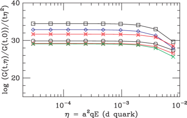
Figure 1: Dependence of $(\log\frac{G_{\pi}(t,\eta)}{G_{\pi}(t,0)})/(t\eta^{2})$ for the neutral pion on a $24^{3}\times 48$ lattice, as a function of $\eta$ for different correlator times. This quantity is roughly equivalent to the shift in the effective mass divided by $\eta^{2}$, and should be constant in the range where $\eta$ creates a purely quadratic effect.

II.3 Extracting the energy shift

To determine the energy shift caused by the external electric field, we compute hadron correlators $G(t,{\mathcal{E}}_{x})$ for positive, zero, and negative values of $\mathcal{E}_{x}$. This requires the computation of five quark-line propagators: one at $\eta=0$, used for both up and down quarks in the case of $\mathcal{E}_{x}=0$, two at $\eta=\pm\frac{1}{3}a^{2}\mathcal{E}_{x}$ for the down quark, and two at $\eta=\mp\frac{2}{3}a^{2}\mathcal{E}_{x}$ for the up quark.

The energy shift caused by the external electric field is quite small, smaller than the stochastic error in the hadron energy itself. Thus, in order to resolve it, we must take into account the fact that the correlators measured with and without the electric field are strongly correlated, and only become more strongly correlated as the strength of the electric field is decreased. We cannot simply, then, do independent correlator fits to the three correlators. Just as an ordinary correlator fit must take into account the correlations between $G(t)$ at different $t$ by computing the covariance between them, we must construct a covariance matrix which includes the mixed covariance between zero-field and nonzero-field correlators. This is simply an extension of the standard fitting procedure using the covariance between all pairs of observables.

We then fit all the data at once, using the fit form

$$\left\langle G(t,\eta)\right\rangle_{\eta}=(A+\Delta A)e^{-(E+\Delta E)t}\,,$$ (3)

to extract $E$ and the parameter $\Delta E$ which is related to $\alpha$. For details on determining the polarizability from the energy shift, see Lujan:2014kia .

For small values of $\mathcal{E}_{x}$, the covariance matrix is quite poorly conditioned due to the extremely strong correlations. We have observed that in this case both the minimization of $\chi^{2}$ and the inversion of the covariance matrix must be done in extended precision to get consistent fit results. For $\eta_{d}=10^{-4}$, we find that the C long double type offers sufficient precision.

III Reweighting

III.1 General remarks

As mentioned previously, the simplest way to incorporate the effect of the electric field on the sea quarks would be to include its effects in gauge generation where the sea dynamics are simulated. However, generating a separate Monte Carlo ensemble to compute the correlator in the presence of background field would ruin the correlations which are necessary to achieve a small overall error. Thus, we turn to reweighting as a method of creating two ensembles which have different sea-quark actions yet are correlated. A similar approach has been used before to compute the strangeness of the nucleon using the Feynman-Hellman theorem Ohki:2009mt , which requires a measurement of $\frac{\partial M_{N}}{\partial m_{s}}$.

Reweighting involves a simple modification of Monte Carlo sampling. Normally, the configurations are sampled using a probability proportional to $e^{-S}$. Then a Monte Carlo estimate for the expectation value of the correlator $G(t)$

$$\left\langle G(t)\right\rangle_{0}\equiv\frac{\int\mathop{{\cal D}\hbox{U}}G(t){e^{-S_{0}}}}{\int\mathop{{\cal D}\hbox{U}}{e^{-S_{0}}}}\approx\frac{1}{N_{\text{confs}}}\sum_{i=1}^{N_{\text{confs}}}{G(t)_{i}}\,.$$ (4)

If we instead want to simulate the physics of a different action $S_{\eta}$ (in our case, with the background electric field) but have access to Monte Carlo configurations using the action $S_{0}$, we can simply modify the Monte Carlo estimate to correct for the additional portion of the factor $e^{-S}$:

$$\left\langle G(t,\eta)\right\rangle_{\eta}=\frac{\left\langle G(t,\eta)e^{-(S_{\eta}-S_{0})}\right\rangle_{0}}{\left\langle e^{-(S_{\eta}-S_{0})}\right\rangle_{0}}\approx\frac{\sum_{i}{G(t,\eta)_{i}w_{i}}}{\sum_{i}w_{i}}\,,$$ (5)

where $\left\langle\cdot\right\rangle_{0}$ indicates the average with respect to $e^{-S_{0}}$ and $w_{i}\equiv e^{-(S_{\eta}-S_{0})}$ is the reweighting factor associated with configuration $i$.

The contribution to the weight factor from the fermion sector, using the standard prescription where the fermions are integrated out, can be written as a ratio of fermion determinants:

$$w_{i}=\frac{\det M_{\mathcal{E}}(U_{i})}{\det M_{0}(U_{i})}\,.$$ (6)

We want to include the effect of the electric field on both flavors of sea quarks; this can be done by simply computing weight factors at two values of $\eta$ (corresponding to the up and down quark charges) and multiplying them.

There are two well-known problems associated with reweighting. The first is that if the overlap between the target and simulated ensemble is poor, the weight factor fluctuates too strongly and the reweighted ensemble will wind up dominated by just a few configurations, leading to a lack of statistical power. The second is that the determinant ratio must be estimated stochastically. The good news is that the since the average over stochastic noises commutes with the gauge average, any unbiased estimator for the weight factor will also produce an unbiased estimate for operators computed on the reweighted ensemble Hasenfratz:2008fg , even if it is quite noisy.

When the reweighting factors are close to one, the overlap is good and for most estimators the stochastic noise is also reduced. Since we can get the reweighting factors arbitrarily close to one by decreasing the value of $\eta$, none of the issues mentioned above create problems for our calculation. On the other hand, this does not mean that our calculation gets more precise as $\eta\to 0$. This is because the signal we try to measure is encoded in the correlation between the weight factor and the ones in the hadronic correlator. As $\eta$ is decreased both signal and error decrease in concert, leading to a constant relative error.

III.2 Perturbative reweighting

As we will see, the most difficult part of performing the reweighting calculation for the electric field is the estimation of the weight factors, as the stochastic estimators for the weight factor in our case are substantially more noisy than in the traditional mass reweighting.

Stochastic estimators for determinant ratios have been used in many studies, more recently as a technique to fine-tune the quark mass in dynamical simulations via reweighting Ohki:2009mt ; Hasenfratz:2008fg ; Liu:2012gm . We attempted at first to use a similar method to estimate the weight factors. However, even for large numbers of stochastic noises, we were unable to resolve even the difference of the weight factors from unity on a production-sized lattice Freeman:2012cy .

In this study we use an alternative to the standard stochastic estimator, a perturbative technique for estimation of the weight factor. Since we are interested only in perturbatively small $\bf\mathcal{E}$, we can expand the one-flavor weight factor $w_{q}$ about $\eta=0$:

$$w_{q}(\eta)=1+\eta\left.\frac{\partial w_{q}}{\partial\eta}\right|_{\eta=0}+\frac{1}{2}\eta^{2}\left.\frac{\partial^{2}w_{q}}{\partial\eta^{2}}\right|_{\eta=0}+\mathcal{O}(\eta^{3})\,.$$ (7)

To obtain the two-flavor weight factor $w$ at some particular value of $\bf\mathcal{E}$ corresponding to $\eta_{d}$ for the down quark and $-2\eta_{d}$ for the up quark, we simply multiply, keeping terms only up to $\eta^{2}$:

$$\begin{split}w(\eta_{d})&=w_{d}w_{u}=w_{q}(\eta_{d})w_{q}(-2\eta_{d})\\ &=1-\eta_{d}\frac{\partial w_{q}}{\partial\eta}+\eta_{d}^{2}\left[\frac{5}{2}\frac{\partial^{2}w_{q}}{\partial\eta^{2}}-2\left(\frac{\partial w_{q}}{\partial\eta}\right)^{2}\right]\,.\end{split}$$ (8)

The derivatives are computed for $\eta_{d}=0$. To simplify notation, we will denote the derivatives with respect to $\eta$ around $0$ as $w_{q}^{\prime}$ and $w_{q}^{\prime\prime}$. Given estimates of these derivatives, we can evaluate the above at any sufficiently-small $\eta_{d}$ to produce a reweighted ensemble on which to apply the valence calculation. This is a semi-perturbative calculation, since the sea effects are introduced perturbatively via the perturbative estimates of the weight factors, but these weight factors are evaluated at finite $\eta_{d}$ and used as inputs to the valence calculation. This differs from the full-perturbative method introduced by Engelhardt Engelhardt:2007ub ; Engelhardt:2010tm in that the hadron correlators are computed non-perturbatively, for a small value of $\eta$. This allows one list of weight factors to be applied to a variety of hadrons, which would not be possible in a fully perturbative calculation. Since determination of the weight factors requires the majority of the computational effort, the numerical effort is greatly reduced when computing the polarizability for a set of hadrons.

Note that we did not include a contribution from the strange quarks in the perturbative expansion. In part this is because the strange sea quarks were not included in the measure used to generate our gauge configurations. Additionally, to include the correction due to the electric charge of the sea strange quarks requires evaluating the derivatives $w^{\prime}_{s}$ and $w^{\prime\prime}_{s}$ for a different quark mass, significantly increasing the numerical effort, while their contribution is expected to be extremely small.

While we are looking only for quadratic effects and expect no shift in the neutron mass proportional to $\eta_{d}$ (due to reflection symmetry), these can arise in two ways: either by the sole effect of the quadratic term in the weight factor, or by a correlation between the first-order term in the weight factor with a similar linear effect in the neutron correlator. The latter occurs because reflection symmetry is not preserved configuration by configuration, but only in the gauge average. We expect that the gauge average of $w_{q}^{\prime}$ is zero, but on individual configurations it will be nonzero.

To evaluate the derivatives we can use Grassman integral techniques and we get

$$w_{q}^{\prime}=\frac{\partial}{\partial\eta}\frac{\det M_{\eta}}{\det M_{0}}=\mathop{\hbox{Tr}}\left(M^{\prime}M_{0}^{-1}\right)\,,$$ (9)

and

$$\begin{split}w_{q}^{\prime\prime}=&\frac{\partial^{2}}{\partial\eta^{2}}\frac{\det M_{\eta}}{\det M_{0}}=\mathop{\hbox{Tr}}\left(M^{\prime\prime}M_{0}^{-1}\right)\\ &+\left(\mathop{\hbox{Tr}}M^{\prime}M_{0}^{-1}\right)^{2}-\mathop{\hbox{Tr}}\left(M^{\prime}M_{0}^{-1}\right)^{2}\,,\end{split}$$ (10)

where $M^{\prime}$ and $M^{\prime\prime}$ are the derivatives with respect to $\eta$ at $\eta=0$ of the one flavor fermionic matrix $M$.

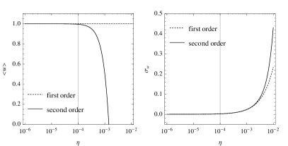
Figure 2: Dependence of the mean and standard deviation of the reweighting factor as a function of $\eta$ for the $24^{3}\times 48$ ensemble used in this study. The estimator is computed using Eq. 8. The solid lines include the quadratic effects in $\eta$, whereas the dotted lines include only the linear term. Vertical lines indicate the $\eta$ value we used.

Once the derivatives are computed, we can use them to determine the values of $\eta$ that are in the small field region. Since we do a perturbative expansion, we want to make sure that the higher order terms are not important. It may seem that given that we only keep the terms of interest, we can set $\eta$ to any value – the higher order terms are not present. On another hand, the reweighting is successful only when $\left\langle w\right\rangle$ is close to one. If we choose values of $\eta$ that are too large, the individual reweighting factors could even go negative. In fact, we can choose $\eta$ such that $\left\langle 1+w^{\prime}\eta+w^{\prime\prime}\eta^{2}/2\right\rangle=0$. It is unclear that the results of the reweighting are meaningful in this case. To set bounds on the $\eta$ value we used as a guiding principle the requirement that the Taylor expansion of $w(\eta)$ is a good approximation.

For the Taylor expansion to be successful, we expect that the successive terms in the expansion are subdominant. We ask then that $\eta$ be such that $1\gg w^{\prime}\eta\gg w^{\prime\prime}\eta^{2}/2$. In Fig. 2 we show both the mean $\left\langle w\right\rangle$ and standard deviation $\sigma_{w}$ for our ensemble as a function of $\eta$ when using the first and second order approximations for $w$. The mean $\left\langle w\right\rangle$ when including only the first order term is close to one for all values of $\eta$ since $\left\langle w^{\prime}\right\rangle\approx 0$, as demanded by symmetries. Note that the mean when including the quadratic term in the approximation deviates quickly from one as we increase $\eta$. This is due to the large value of $\left\langle w^{\prime\prime}\right\rangle$. In fact, a large constant $\left\langle w^{\prime\prime}\right\rangle$ is not important since it cancels out in the reweighting ratio from Eq. 5. The fluctuations of $w$ about the mean are important and that is why we plot $\sigma_{w}$ as a function of $\eta$. Note that the standard deviation is dominated by the first order term for values of $\eta$ much larger than the ones where the mean deviates from one. In any case, the value of $\eta=10^{-4}$ used in this study is well inside the region where the Taylor expansion is working well.

IV Stochastic estimations of the weight factor

The traces that appear in the expressions for the determinant derivatives, Eqs. 9 and 10, can be evaluated stochastically in the standard way, that is

$$\mathop{\hbox{Tr}}\mathcal{O}=\left\langle\xi^{\dagger}\mathcal{O}\xi\right\rangle_{\xi}\,,$$ (11)

where $\xi$ are Z(4) noise vectors. We note that only three estimators are required—$\mathop{\hbox{Tr}}M^{\prime}M_{0}^{-1}$, $\mathop{\hbox{Tr}}M^{\prime\prime}M_{0}^{-1}$, and $\mathop{\hbox{Tr}}(M^{\prime}M_{0}^{-1})^{2}$—since an estimator for $\left[\mathop{\hbox{Tr}}(M^{\prime}M_{0}^{-1})\right]^{2}$ can be constructed from two uncorrelated values of the estimator for the first-order term $\mathop{\hbox{Tr}}(M^{\prime}M_{0}^{-1})$. As $\left[\mathop{\hbox{Tr}}(M^{\prime}M_{0}^{-1})\right]^{2}$ is both computed separately and subdominant, we refer to the combination of the two second-order terms that must be explicitly estimated, $\mathop{\hbox{Tr}}(M^{\prime\prime}M_{0}^{-1})-\mathop{\hbox{Tr}}(M^{\prime}M_{0}^{-1}M^{\prime}M_{0}^{-1})$, as ${\tilde{w}}_{q}^{\prime\prime}$. Note that there is no bias introduced by using the same stochastic noise vector for the $w_{q}^{\prime}$ and $\tilde{w}_{q}^{\prime\prime}$, since the ultimate computation of the weight factor involves only linear combinations of these estimates; any correlations in the stochastic fluctuations will not cause the final result to be biased. This reduces the number of inversions required per noise vector to two.

Standard stochastic estimators of these traces are, unfortunately, very noisy. For example, on a $4^{4}$ lattice we need $5\times 10^{6}$ noise vectors to obtain a signal-to-noise ration greater than one for the first derivative. In Fig. 3 we compare the stochastic result with the exact result computed via direct evaluation Alexandru:2010yb . We see an agreement between $w_{q}(\eta)$ and the stochastic estimator for $w_{q}^{\prime}$, with the onset of quadratic behavior visible as $\eta$ is increased.

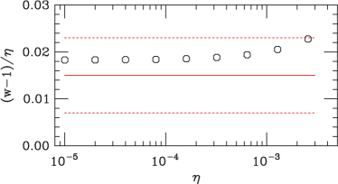
Figure 3: Exact values for $[w(\eta)-1]/\eta$ on a $4^{4}$ lattice, compared with the value predicted by the stochastic estimator for $w^{\prime}$ and its error band.

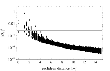
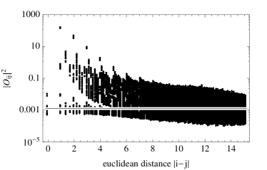
Figure 4: Mapping of a representative set of the off-diagonal elements of $M^{\prime}M_{0}^{-1}$ (left) and $M^{\prime\prime}M_{0}^{-1}-(M^{\prime}M_{0}^{-1})^{2}$ (right). The average of the square of the $12$ diagonal elements, the ones that define the signal, is shown as a horizontal line.

IV.1 Estimator quality

Since the limiting factor for this calculation is the stochastic estimation of the weight factors, it is useful to understand how far we need to reduce the variance in the stochastic estimator. Whether using perturbative or nonperturbative reweighting, it is the variation of the weight factor between gauge configurations that carries the information, and it is this fluctuation that we seek to extract using a stochastic estimator. Thus the gauge variance between configurations in the weight factor amounts to a signal, while the stochastic variance gives the noise in that signal. This immediately suggests a criterion for judging the quality of any given stochastic estimation scheme: the stochastic signal-to-noise ratio

$$w_{\mathrm{S}NR}\equiv\frac{\sigma_{\rm gauge}}{\sigma_{\rm noise}}\,.$$ (12)

Ideally we would like this SNR to be as large as possible. A SNR substantially less than unity means that the stochastic estimator scheme used is insufficient to extract whatever physics differences exist between the original and reweighting ensembles. In our case, this may be because the actual difference is small, or because the estimator is too noisy; the only way to determine which is to carry the calculation to its conclusion and see how much reweighting increases the overall error bar.

There are two difficulties which make this SNR a guideline, rather than a quantitative measurement:

1. Determining the gauge variance is difficult, since it requires knowledge of the true weight factors, the same quantities whose estimation we are concerned with.

2. When using a highly diluted estimator (which we will choose to use in the end), determination of the stochastic variance requires computation of multiple stochastic estimates. This may involve a substantial amount of computer power.

We will return to these issues later in the discussion of specific estimators in Sec. IV.2.

IV.2 Mapping the stochastic noise

It can be shown readily that the variance of the stochastic estimator $\mathop{\hbox{Tr}}\mathcal{O}=\left\langle\xi^{\dagger}\mathcal{O}\xi\right\rangle$ is

$$\left\langle(\xi^{\dagger}\mathcal{O}\xi)^{2}\right\rangle-\left\langle\xi^{\dagger}\mathcal{O}\xi\right\rangle^{2}=\sum\limits_{i\neq j}|\mathcal{O}_{ij}|^{2},$$ (13)

the sum of the squares of the off-diagonal elements of $\mathcal{O}$. Understanding which of these elements dominate is useful for designing improvements to the stochastic estimator. As we cannot even afford to compute all of the diagonal elements (to get an exact value for $\mathop{\hbox{Tr}}\mathcal{O}$), we certainly cannot compute all of the $\mathcal{O}_{ij}$’s. However, we can examine a representative set to see which are dominant. On a single configuration from our $24^{3}\times 48$ ensemble, we have computed all $\mathcal{O}_{ij}$ for a set of sources $j$

$${\cal S}=\left\{j|j_{x,y,z}\in\{8,16\}\,,j_{t}\in\{16,24,32\}\right\}\,.$$ (14)

Since we compute all spin-color combinations, the number of sources is $|{\cal S}|=12\times 24=288$. We kept the information only for sinks $i$ such that the vector between $i$ and $j$ has no components larger than 12 (after accounting for periodic boundary conditions in the $y$ and $z$ directions). The number of data points is very large and to produce a more manageable set we bin the points in equivalence classes. For the purpose of this illustration, we assume that all source positions are equivalent, so we average together the squares of all matrix elements corresponding to different source points. We notice no significant effects on matrix elements whose sinks are near the Dirichlet boundary, so we bin together the points where the separation vector between $i$ and $j$ is related by a reflection in any direction or rotation in the $(y,z)$-plane. We also bin together the points that have the same starting and ending color indices and separately the ones that have different color indices. We treat the directions $x$ and $t$ separately due to the effects of the electric field and collect each of the 16 spinor combinations in a separate bin. All these data points are used to create Fig. 4 and to predict the error of the stochastic estimators for different dilution schemes.

The relative size of the off-diagonal elements as a function of the Euclidean separation between $i$ and $j$ is shown in Fig. 4 for both $M^{\prime}M_{0}^{-1}$, the first-order term, and $M^{\prime\prime}M_{0}^{-1}-(M^{\prime}M_{0}^{-1})^{2}$, the second order term. We note that the magnitude of $|\mathcal{O}_{ij}|^{2}$ decreases as $i$ and $j$ are further apart, as expected. The short-range behavior is the source of our problem. The trace estimator we use works well for diagonally dominated matrices, where the largest elements of the matrix lie along the diagonal, and decay quickly as we go away from it. Unfortunately, for our matrices the dominant elements are not on the diagonal, as can be easily seen from Fig. 4. Even among the elements at Euclidean separation 0, those off-diagonal elements $\mathcal{O}_{ij}$ where $i$ and $j$ differ in spin and color indices are larger than the diagonal elements. This is a simple depiction of why this stochastic estimator is so difficult: the diagonal elements (the signal) are small, while the near-diagonal elements contributing to noise are much larger. The structure is not unexpected, since $M^{\prime}$ amounts to a point-split operator in the $t$ direction.

Fig. 4 suggests that the most direct route to reducing the variance is reducing the short-range off-diagonal elements of the operators. There are two somewhat redundant techniques we can use to do this: hopping parameter expansion improvement and dilution. Hopping parameter expansion has the advantage that its numerical cost is relatively modest for small orders, but it only cancels the off-diagonal elements approximatively. We explored this technique in a previous study using an expansion up to $7^{th}$ order, the largest order we could afford Freeman:2013eta . We found that the improvement was insufficient and the signal-to-noise ratio for polarizability was smaller than one. In this work we explore an alternative approach: dilution.

IV.3 Dilution scheme

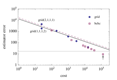
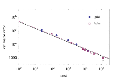
Figure 5: Uncertainty estimates for different dilution schemes for the first-order term (left) and second-order term (right) as a function of the the estimator cost, given by the number of partitions in each dilution scheme. The solid (dashed) line indicates the expected uncertainty for the estimates based on repeated use of the undiluted (spin-color diluted) estimator. The horizontal line in the left panel corresponds to the standard deviation of the gauge fluctuations, as estimated in the next section. The point in the bottom-right labelled by a black arrow is the BCHC-$6^{4}$ dilution scheme actually used in the computation.

Dilution is a technique which, with a suitable dilution scheme, can eliminate the noise contribution from near-diagonal elements. It entails partitioning the lattice into $N$ subspaces, estimating the trace over each separately, and adding the estimates; this is done in practice by generating noise vectors with support only on one subspace. This eliminates contributions to the variance from off-diagonal elements $\mathcal{O}_{ij}$ where $i$ and $j$ belong to different subspaces, at the cost of requiring $N$ evaluations of $\mathcal{O}$ to generate a single estimate. Thus there is a fundamental tradeoff involved in dilution. The aim of any stochastic estimation procedure is to minimize the uncertainty in the stochastic estimate for a given computational effort, and that uncertainty, rather than the variance of the estimator itself, should be used as the yardstick for measuring the utility of a dilution technique.

The variance of the diluted estimator should then be compared with the variance of an estimate based on the average of $N$ independent evaluations of the undiluted estimator. The variance of this mean is smaller by a factor of $N$ than the variance of a single evaluation. To be more precise, if we label the partition to which the (spin/color/spatial) index $i$ belongs as $P(i)$, the variance becomes

$$\mathrm{var}(\mathop{\hbox{Tr}}\mathcal{O})=\sum\limits_{i\neq j}|\mathcal{O}_{ij}|^{2}\delta_{P(i)P(j)},$$ (15)

that is, the sum of only those off-diagonal elements that connect indices belonging to the same subspace. If all $N$ subspaces are of equal size (which is generally the case), then this results in a sum with only $1/N$ as many terms. The ratio of uncertainties (the proper figure of merit) between an $N$-subspace dilution and the mean of $N$ undiluted estimators, is

$$\frac{\sum\limits_{i\neq j}|\mathcal{O}_{ij}|^{2}\delta_{P(i)P(j)}}{\frac{1}{N}\sum\limits_{i\neq j}|\mathcal{O}_{ij}|^{2}}.$$ (16)

Thus dilution will only be a success if the average of the off-diagonal elements that survive (belong to the same subspace) is less than the average of all of them. Choosing a dilution strategy, then, must be done with consideration of the form of $\mathcal{O}_{ij}$, as it is entirely possible to partition the lattice in such a way to make the stochastic noise worse.

The most common sort of dilution is spin/color dilution, where each noise vector has support for a single spin and color over the entire lattice. As we can see from Fig. 5 this dilution scheme alone does not help us; it must be used alongside other dilution schemes in which the subspace structure also involves spatial separation.

To construct the spatial structure for a dilution scheme for an operator whose off-diagonal elements are expected to decrease with increasing Euclidean distance, we want to allocate sites among the $N$ subspaces so as to maximize the minimum Euclidean distance separating two sites belong to the same subspace. We investigate two schemes: regular grid and body-centered hypercubic (BCHC) scheme.

For a regular grid two points belong to the same partition if

$$p_{1}-p_{2}=0\pmod{\Delta}\,.$$ (17)

The four-dimensional vector $\Delta$ defines the steps of the grid in the four spatial directions. The number of partitions, which is proportional to the cost of the dilute estimator, is controlled by the volume of one grid cell $N=\prod_{i}\Delta_{i}$. When used in conduction with the spin-color dilution, we have $N=12\prod_{i}\Delta_{i}$. The minimum Euclidean distance between two points on the same grid is the smallest grid step $\min_{i}\Delta_{i}$.

In the BCHC scheme, two points belong to the same partition if

$$p_{1}-p_{2}\in\{0,\Delta\}\pmod{2\Delta}\,.$$ (18)

This can be thought of as two regular grids of steps $2\Delta$ displaced by vector $\Delta$, so that the origin of the second grid lies in the middle of the unit cell $2\Delta$, creating a body-centered hypercubic pattern with unit cell $2\Delta$. The number of partitions for this scheme is $N=8\prod_{i}\Delta_{i}$, or $N=96\prod_{i}\Delta_{i}$ when spin-color dilution is also used; it is half that of a grid dilution scheme with the same nearest-neighbor distance. The minimal distance between two points from the same partition depends on the relative magnitude of the components of $\Delta$; when all components are the same $\Delta_{i}=b$, the minimal distance is $\left\|{\Delta}\right\|=2b$. Note that for a regular grid we would need $N$ twice as large to achieve this minimal distance.

A disadvantage of large-$N$ dilution strategies is the need for a large numerical effort to compute even a single estimate of the trace, even if that single estimate has greatly reduced stochastic error. This makes it difficult to empirically determine the variance of a large-$N$ dilution scheme by repeated application, because the cost of repeating the estimator enough times to achieve a sufficiently low error on the variance becomes prohibitive. However, we can use the off-diagonal element mapping data to estimate the variance for any dilution scheme. Under the assumptions outlined above, we estimate

$$\mathrm{var}(\mathop{\hbox{Tr}}\mathcal{O})\approx\frac{12\times V_{\text{lat}}}{N}\sum_{i\in V}^{N}\sum_{j\neq i}|\mathcal{O}_{ij}|^{2}\delta_{P(i)P(j)}\,,$$ (19)

where $V_{\text{lat}}$ is the lattice volume and the positions and spin/color of the $N$ sources $i$ are chosen randomly. The sum over the sinks $j$ extends over the entire lattice, rather than a limited hypercube as in Fig. 4, eliminating any effects from small points beyond the horizon on the variance. Additionally, scattering the points over the entire lattice, rather than confining them to a central region away from the Dirichlet walls, correctly incorporates the finite-size effects from the Dirichlet boundary conditions into the estimator variance. For $N$ large enough, the result should quickly converge to the true variance of $\mathcal{O}$. Using 300 randomly chosen lattice points and evaluating all 12 color-spin indices at these points, we determine the standard deviation for our estimators with percent-level error on a few configurations. We find that the standard deviation varies very little from configuration to configuration. The mean value over the configurations is used for the data in Fig. 5.

This is a useful tool to use in planning a dilution scheme. In Fig. 5 we compare the predicted uncertainty for our stochastic estimator using various dilution schemes. Except for the solid line, all estimators use spin-color dilution. As noted before, the spin-color dilution by itself (indicated by the dashed line) is inferior to the undiluted estimator. At first order, moderately-aggressive dilution schemes essentially keep pace with the decline in the estimator variance caused by simple repetition. Dilution begins to win out once the minimum Euclidean distance between adjacent points in the same subspace, reflected in the increasing cost, increases. At second order, only an extremely small improvement is seen; this is due to the substantially slower falloff of the offdiagonal elements seen in Fig. 4. Either a more aggressive dilution scheme or an operator-improvement technique used in tandem with dilution is needed to see much improvement over simple repetition of the naïve estimator.

The BCHC dilution schemes should show at best a reduction in the cost by a factor of $2$ compared to grid schemes, since they achieve the same minimum distance with half as many partitions. The actual gain is less than this, because a grid source has only eight nearest neighbors, while the BCHC source has sixteen. Nonetheless, for both the first and second order estimators, the BCHC dilution outperforms grid dilution by a small amount.

To reduce the stochastic variance to a level comparable with the gauge variance we need a large grid spacing. In the left panel of Fig. 5 we see that this happens for the first-order derivative only when $\Delta=\{6,6,6,6\}$. This is the dilution scheme used in the subsequent calculation. In this scheme, the minimal Euclidean distance between two points in the same partition is $12$ and the number of partitions is $N=96\prod_{i}\Delta_{i}=124,416$.

IV.4 Gauge variance

Off-diagonal element data allows us to determine the expected variance for our estimators. However, it provides no indication as to the level of gauge variance, which we also need to know to determine whether a dilution scheme noise is smaller that the expected signal, as discussed in Section IV.1. To estimate gauge variance we did two tests: an extrapolation from small lattices where we can compute the operators exactly and a more computational intensive study where we evaluated our expensive high quality estimator (BCHC with $\Delta=\{6,6,6,6\}$) on a couple of lattices from our ensemble.

config	$N_{\text{est}}$		$w_{q}^{\prime}$			$\tilde{w}_{q}^{\prime\prime}$
			mean	std-dev		mean	std-dev
2	6		-2.8(2.7)	6.5(2.1)		-196,362(468)	1147(371)
3	4		-19.9(4.7)	9.4(4.0)		-197,399(324)	648(274)

Table 1: Repeated trials of the BCHC diluted estimator for two configurations. The standard deviation field indicates the stochastic error, which we determined in Section IV.3 to be $9.5(6)$ for the first-order estimator and $1038(76)$ for the second-order one.

We discuss first direct evaluation of our estimator on $24^{3}\times 48$ lattices. For the first two lattice configurations in our ensemble we run several evaluations of our estimator. The results of this test are shown in Table 1. We first note that the standard deviation for the stochastic estimators is consistent with the estimate from the previous section. For the first-order term $w_{q}^{\prime}=\mathop{\hbox{Tr}}M^{\prime}M_{0}^{-1}$ the gauge fluctuations are $16(8)$. This estimate takes into account the fact the gauge average is zero, by reflection symmetry, for the first-order term. A correction factor is used to account for the bias in the standard deviation estimator. The stochastic fluctuations are smaller than the gauge fluctuations. This suggests that this estimator is precise enough to follow the gauge fluctuations.

For the second-order term, the gauge average value is $-196,881(491)$. The standard deviation of the gauge fluctuations is $\sigma_{\text{gauge}}=919(694)$, of similar order with the stochastic uncertainty. It is not clear whether the signal-to-noise ratio is good enough for this estimator, especially since our determination is also compatible with small values for the gauge fluctuations. We will see that the extrapolation from small volumes predicts that $\sigma_{\text{gauge}}$ is on the small side of the estimate. This suggests that the second order estimator is noisy. Note that the cost of this seemingly-simple study is 2.5 million inversions, about $3\%$ of the cost of the entire calculation.

We turn now to the extrapolation from small volumes. We generated a set of small lattice of different geometries and computed the first and second order derivatives exactly using the compression method for Wilson fermions Alexandru:2010yb ; Nagata:2010xi . More precisely, we computed the fermionic determinant on these lattices exactly for $7$ different values of the electric field parameter $\eta$ and then evaluated the derivatives numerically using a $\mathcal{O}(\eta^{6})$ finite difference scheme

$$f^{\prime}\approx\frac{1}{\eta}\sum_{k=-3}^{3}c^{\prime}_{k}f(k\eta)\,,\kern 5.0ptf^{\prime\prime}\approx\frac{1}{\eta^{2}}\sum_{k=-3}^{3}c^{\prime\prime}_{k}f(k\eta)\,,$$ (20)

where $f(\eta)=\log\det M(\eta)$. It is straightforward to relate these derivatives to the derivatives of the reweighting factor: $w^{\prime}_{q}=f^{\prime}$ and $\tilde{w}^{\prime\prime}_{q}=f^{\prime\prime}$. The coefficients for these approximations are given in Table 2. We use a value of $\eta=0.01$ which is sufficiently precise.

$k$		-3	-2	-1	0	1	2	3
$c_{k}^{\prime}$		-1/60	3/20	-3/4	0	3/4	-3/20	1/60
$c^{\prime\prime}_{k}$		1/90	-3/20	3/2	-49/18	3/2	-3/20	1/90

Table 2: Coefficients for the finite difference derivatives.

For each lattice geometry we generated 10 configurations. We used Wilson pure gauge action with $\beta=6.0$. The lattice spacing is $a/r_{0}=0.186$ Necco:2001xg , which is similar to the lattice spacing for our large configurations. For the fermionic matrix, we use nHYP fermions with $\kappa=0.1267$. The parameter $\kappa$ was adjusted to produce a pion mass around $300\,{\rm MeV}$ to match the sea quark mass on the large configurations.

To make sure that we are not in the deconfined phase, we have to keep $r_{0}/L<r_{0}T_{c}=0.7498(50)$ Necco:2003vh . This means that all of our lattice dimensions $n_{i}=L_{i}/a$ should satisfy $n_{i}\geq 8$. Since this is already at the upper range of lattice volumes where we can compute the determinant exactly, to investigate a wider range of volumes we have to use geometries that do not satisfy this constraint. For these lattices, we take advantage of the Dirichlet boundary conditions in the $x$ and $t$ directions and cut out these lattices from larger ones, with $n_{x}=n_{t}=12$, that are in the confined phase. The only delicate step in this process is that we have to smear the links on the larger lattice and then cut it, so that the boundary do not introduce discontinuities. We use 72 different lattice geometries: $n_{y},n_{z}\in\{8,10,12\}$, $(n_{x}|n_{t})\in\{4|4,4|6,6|4,4|8,8|4,4|10,10|4,6|6\}$.

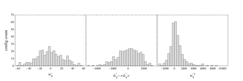
Figure 6: Distribution of the values of the stochastic estimators on the full 300-configuration ensemble. The two leftmost panels are the stochastic estimators for $w_{q}^{\prime}$ and $\tilde{w}^{\prime\prime}_{q}$ using BCHC dilution. The right panel is the estimator for $w_{q}^{\prime 2}$ using a combination of BCHC-dilution and hopping parameter expansion estimators, as described in the text. Note that for the center panel we shifted the distribution by subtracting its mean.

For each ensemble we determine the gauge standard deviation for both derivatives and mean for the second derivative. We analyzed the dependence of each of these three quantities as we varied the dimension of the lattice in each direction. In most cases we found that these quantities vary linearly with the dimension (either relatively constant or raising linearly). The only exception is the mean of the second order derivative which requires quadratic terms to describe its dependence on $n_{x}$, the extent of the lattice in the direction of the external field. Based on these observations and taking into account the rotational symmetry in the $(y,z)$-plane, the fit functions we use in our extrapolations are

$$\begin{split}\sigma_{w_{q}^{\prime}}&=\alpha(n_{x}+\beta_{x})(1+\gamma n_{y})(1+\gamma n_{z})(n_{t}+\beta_{t})\,,\\ \left\langle\tilde{w}_{q}^{\prime\prime}\right\rangle&=\alpha(n_{x}+\beta_{x}+\gamma n_{x}^{2})n_{y}n_{z}(n_{t}+\beta_{t})\,,\\ \sigma_{\tilde{w}_{q}^{\prime\prime}}&=\alpha(n_{x}+\beta_{x})(1+\gamma n_{y})(1+\gamma n_{z})(n_{t}+\beta_{t})\,.\end{split}$$ (21)

The results of the fits are presented in Table 3. Using these coefficients and their cross-correlations, we estimate that for a $24^{3}\times 48$ lattice the gauge averages and standard deviations should be

$$\begin{split}\sigma_{w^{\prime}_{q}}&=17(4)\,,\\ \left\langle\tilde{w}^{\prime\prime}_{q}\right\rangle&=-212(2)\times 10^{3}\,,\\ \sigma_{\tilde{w}_{q}^{\prime\prime}}&=164(62)\,.\end{split}$$ (22)

We note that all these results are compatible with the values determined via repeated evaluation of the stochastic estimator on two full-size configurations. As we mentioned earlier, the gauge standard deviation for $\tilde{w}^{\prime\prime}_{q}$ is lower than the stochastic uncertainty, indicating a noisy estimator.

		Q	$\alpha$	$\beta_{x}$	$\beta_{t}$	$\gamma$
$\sigma_{w_{q}^{\prime}}$		0.15	0.0017(10)	-1.6(3)	1.9(1.2)	0.08(4)
$\left\langle\tilde{w}_{q}^{\prime\prime}\right\rangle$		0.85	-0.09(2)	-3.95(3)	-1.61(7)	0.118(5)
$\sigma_{\tilde{w}_{q}^{\prime\prime}}$		0.27	0.09(3)	-3.1(1)	3(2)	0.014(16)

Table 3: Fit parameters for extrapolation from small volumes. Q is the confidence level of the fit.

V Results

V.1 Reweighting factors

Before we turn to the main results in this paper, hadron polarizabilities, we present the results for the reweighting factors, as evaluated on the full ensembles using the estimators described in the previous section.

The resulting estimates for $w^{\prime}_{q}$, $\tilde{w}^{\prime\prime}_{q}$, and $(\mathop{\hbox{Tr}}M^{\prime}M_{0}^{-1})^{2}$ are given in Fig. 6. We discuss here briefly the estimator for $w_{q}^{\prime 2}=(\mathop{\hbox{Tr}}M^{\prime}M_{0}^{-1})^{2}$. When more than one estimate per configuration of the first-order term $w_{q}^{\prime}$ is available, such as in the previous study using hoping parameter expansion improvement where we used thousands of cheap estimators per configuration Freeman:2013eta , we may construct one estimate for $w_{q}^{\prime 2}$ out of two independent estimates of $w_{q}^{\prime}$. However, in this study we used an expensive BCHC-diluted estimator and there is no second estimate of $w_{q}^{\prime}$ available. Constructing a second one in the same manner as the first, using the $N=124,416$ dilution scheme, would require a large extra effort. However, we observed from the previous study that the stochastic fluctuations of this term compared to the fluctuations of the rest of the traces involved in $\tilde{w}_{q}^{\prime\prime}$ are small. Thus it is acceptable to use a less labor-intensive method to estimate it. Since we have the estimates of $w_{q}^{\prime}$ from the prior run saved to disk, we use them in combination with the new diluted estimates of $w^{\prime}_{q}$ to produce an estimate of $w_{q}^{\prime 2}$ on each configuration.

For the first order term we find that the standard deviation is $\sigma_{w_{q}^{\prime}}=23(1)$. This includes both the stochastic noise and the gauge fluctuations. The determination is compatible with our estimates described in the previous section. For the second order term, $\tilde{w}_{q}^{\prime\prime}$, the mean value is $\left\langle\tilde{w}_{q}^{\prime\prime}\right\rangle=-197,549(83)$ and the standard deviation is $\sigma_{\tilde{w}_{q}^{\prime\prime}}=1429(58)$, again in agreement with the values estimated in the previous section. We note that the combined standard deviation is larger than the gauge one estimated from the extrapolation from small volumes, indicating that the stochastic noise is dominant for this estimator.

For the $w_{q}^{\prime 2}$ estimator we find that the standard deviation is $\sigma_{w_{q}^{\prime 2}}=1655(68)$. This is comparable with the standard deviation for $\tilde{w}_{q}^{\prime\prime}$ and it would seem that this term will add significant variance to the final result. To see why this term is subdominant we have to expand Eq. 8 in terms of traces:

$$w(\eta_{d})=1-\eta_{d}w_{q}^{\prime}+\frac{1}{2}\eta_{d}^{2}\left(5\tilde{w}_{q}^{\prime\prime}+w_{q}^{\prime 2}\right)\,.$$ (23)

We see that in the final result, the quadratic term $w^{\prime\prime}=5\tilde{w}_{q}^{\prime\prime}+w_{q}^{\prime 2}$ is dominated by $\tilde{w}_{q}^{\prime\prime}$. Indeed the total standard deviation for the quadratic term is $\sigma_{w^{\prime\prime}}=7231(295)$, compared to the contribution coming from $\tilde{w}_{q}^{\prime\prime}$ alone, $5\times\sigma_{\tilde{w}_{q}^{\prime\prime}}=7147(292)$.

		Valence only				$1^{\text{st}}$ order				$\tilde{w}_{q}^{\prime\prime}$ only				$2^{\text{nd}}$ order
		$aE$	$a\Delta E$	$Q$		$aE$	$a\Delta E$	$Q$		$aE$	$a\Delta E$	$Q$		$aE$	$a\Delta E$	$Q$
Pion		0.245(1)	-5.4(3.4)	0.17		0.245(1)	-6.0(3.4)	0.18		0.245(1)	5.4(5.6)	0.15		0.245(1)	5.6(5.7)	0.15
Kaon		0.352(1)	4.2(0.8)	0.12		0.352(1)	3.7(1.0)	0.07		0.352(1)	10.5(3.4)	0.03		0.352(1)	11.1(3.4)	0.02
Neutron		0.694(4)	62.8(5.7)	0.65		0.694(4)	63.9(6.5)	0.57		0.695(4)	72.5(16.4)	0.53		0.695(4)	67.0(16.3)	0.43

Table 4: Results for the energy and energy shift for the pion, neutron, and kaon with differing orders of reweighting: none (the valence-only calculation), first-order in $\eta_{d}$, second-order including only the dominant contribution in $\tilde{w}_{q}^{\prime\prime}$, and the full calculation to second order. For the energy shifts, the values are in units of $10^{-8}$. $Q$ is the confidence level for the fits corrected to account for the sample size Toussaint:2008ke .

V.2 Hadron polarizabilities

The power series expansion given in Eq. 8 can be used to determine the weight factor at any desired $\eta_{d}$ on each configuration; these weight factors can then be combined with the valence correlators computed previously to complete the calculation. We note that one set of weight factor estimates may be used without modification for all hadrons; this is a strength of the reweighting approach. Full details of the valence correlators are given in Lujan:2014kia ; we repeat only the essential elements here. We use point interpolators for both source and sink. To improve the signal-to-noise ratio, we use 28 sources per configuration; in any case the expense of the many sources is dwarfed by the cost of the weight factor estimates. These sources are spread evenly in the $(y,z)$-plane but are along the centerline $x=12$ to avoid the Dirichlet walls.

It is informative to turn on the reweighting one order at a time; we additionally add the extra second-order term, $w_{q}^{\prime 2}$, separate from the others that comprise $\tilde{w}_{q}^{\prime\prime}$. Using these approximations for the reweighting factors we compute the hadron propagators using Eq. 5 and do a correlated fit for zero field and non-zero field propagators using the model in Eq. 3. The fit ranges for these fits are the same as in our previous valence study Lujan:2014kia . The results for these fits are presented in Table 4. Focusing on the energy shift, $a\Delta E$, note that the uncertainty remains relatively constant when including only the first order terms, indicating that our estimator adds very little noise. The second order term, in particular $\tilde{w}_{q}^{\prime\prime}$, introduces significantly more uncertainty, doubling or trebling the size of the error bars. In principle this could be due to either the gauge fluctuations of the second-order term causing a large fluctuation in the weight factor. However, in our case the estimated stochastic error for $\tilde{w}_{q}^{\prime\prime}$ is fairly large compared to the overall variation of the estimator, so we suspect that the largest share of the fluctuations in our estimates are due to stochastic noise, despite the substantial effort involved in the estimator. As discussed previously, the addition of the $w_{q}^{\prime 2}$ estimate has very little effect both on the value of the energy shift and its error.

To convert the energy shift to polarizability we use the relation:

$$\alpha=\frac{2a^{3}e^{2}}{9\eta_{d}^{2}}(a\Delta m)=\frac{2a^{3}e^{2}}{9\eta_{d}^{2}}\frac{aE}{aM}(a\Delta E)\,,$$ (24)

where $M$ is the mass of the hadron of interest, computed using periodic boundary conditions. These masses were computed for this ensemble in a previous study Lujan:2014kia . For the neutron a correction due to the magnetic moment is required, $\alpha_{c}=\alpha+\mu^{2}/(2m)$ Lvov:1993fp ; Detmold:2010ts ; Lujan:2014kia . The polarizability values are given in Table 5. We will discuss now each hadron separately.

		Valence only	$1^{\rm{St.}}$ order	$\tilde{w}_{q}^{\prime\prime}$ only	$2^{\rm{nd}}$ order
Pion		-0.21(14)	-0.24(14)	0.21(22)	0.22(23)
Kaon		0.14(3)	0.13(3)	0.36(12)	0.38(12)
Neutron		2.56(19)	2.60(22)	2.89(55)	2.70(55)

Table 5: Electric polarizability for the pion, neutron, and kaon with differing orders of reweighting: none (the valence-only calculation), first-order in $\eta_{d}$, second-order including only the dominant contribution in $\tilde{w}_{q}^{\prime\prime}$, and the full calculation to second order. Values are in units of $10^{-4}\,{\rm fm}^{3}$.

We remind the reader that the neutral pion correlator used in this study does not include the disconnected diagrams that are required due to the isospin breaking introduced by the electric field. This is a common limitation for lattice calculations, since the inclusion of these terms is computationally expensive. For the neutral pion, chiral perturbation theory predicts a polarizability around $\alpha_{\pi^{0}}\approx-0.5\times 10^{-4}\,{\rm fm}^{3}$. In the absence of the disconnected contributions, the prediction is that the polarizability would be positive and an order of magnitude smaller in absolute value Detmold:2009dx . Lattice calculations of this quantity indicate that the connected neutral pion polarizability turns negative as the pion mass is lowered below $400\,{\rm MeV}$, contradicting these expectations Detmold:2009dx ; Alexandru:2010dx ; Lujan:2014kia . It was suggested that this discrepancy is due to final volume corrections Detmold:2009dx , but this does not seem to be the case Alexandru:2010dx . The correction associated with charging the sea quarks might also be responsible for this discrepancy. As we can see from Table 5, the polarizability for the neutral pion seems to change signs as we charge the sea quarks. However, the current errors are too large, relative to the size of polarizability, so no definitive conclusions can be drawn. We also measured the change in the energy shift induced by the reweighting taking into account the correlations between the original and reweighted measurements; the result was consistent with zero. We note that the valence-only result is very close to zero; the ensemble in question happens to lie very near the value of $m_{\pi}$ where the polarizability of the neutral pion changes sign Alexandru:2010dx ; Lujan:2014kia .

Neutral kaon polarizability is not shifted by the first order reweighting. When the second order is included, both the central value and its uncertainty increase. In this case the shift in polarizability is statistically significant. It is interesting to note that this behavior is consistent with the features we observed in our previous study: kaon polarizability was insensitive to the change in mass of the valence light quarks, but it shifted significantly when the mass of the light sea quarks was changed Lujan:2014kia . This was in contrast with the pion polarizability which seems to depend strongly on the valence quark mass, but it was fairly insensitive to the sea. It is then not surprising that the kaon polarizability should be sensitive to charging the light sea quarks. In any case, the chiral extrapolation performed in our previous study for kaon polarizability needs to be revisited, given the significant shift induced by charging the sea.

The neutron, the benchmark hadron for this type of calculations, shows no statistically significant change when the coupling to the sea is turned on via reweighting. This is a bit puzzling since the chiral perturbation theory expectation is that the neutron polarizability increases by $1$–$2\times 10^{-4}\,{\rm fm}^{3}$ when the sea quarks are charged Detmold:2006vu and our errorbars, even after including the second order correction, are small enough to resolve this difference. It is still possible that this increase shows up after removing the finite volume effects, that are expected to be significant for this quantity. We note that our calculation of neutron polarizability, including sea effects, improves upon the precision of the only other such calculation known to us Engelhardt:2007ub ; Engelhardt:2010tm in both precision and pion mass.

While the effects of charging the sea quarks are not statistically significant here, with the exception of the kaon, we expect them to be enhanced both by enlarging the lattice volume and by approaching the chiral limit. Considering the chiral limit: when the pion mass is reduced it is easier to create virtual pion loops which increases the size of the pion cloud and its contribution to polarizability. Similarly, increasing the size of the box reduces the momentum of the lowest pion state (recall that we use Dirichlet boundary conditions), reducing the cost of exciting pions, with similar consequences. We thus expect the effect of charging the sea to be substantially larger at lower pion mass and on larger boxes.

VI Conclusion

While the result for the neutron here is physically significant, as it improves on the previously-attained precision, we treat it more of a proof of concept for the perturbative reweighting method which will soon be applied to ensembles with larger volumes and smaller pion masses, where we expect the effect to be larger. The perturbative estimate for the weight factor correctly predicts the slope of the exact determinant ratio on small lattices where it can be computed exactly, but like the conventional reweighting estimator it is quite noisy. However, dilution can be used to reduce its variance. Strong dilution with the body-centered hypercubic pattern outperforms hopping parameter expansion and it is certainly simpler to formulate and more flexible.

Our results suggest that while these estimates of the first-order term $w^{\prime}_{q}$ are sufficient, a reduction in the stochastic noise from the second-order term would be welcome, given that the other ensembles in the study will be inherently more expensive. Dilution completely eliminates the near-diagonal contributions, at the cost of indirectly increasing the contributions away from the diagonal since we no longer average together many estimates. The long-distance behavior of the off-diagonal elements is exponential and its slope is governed by $m_{\pi}$. We are exploring the use of low-mode subtraction to eliminate the lowest lying modes of the Dirac operator from the operators in question and thus increase the exponent of the falloff; preliminary studies of this technique look promising.

- (1) J. Schmiedmayer, P. Riehs, J. A. Harvey, and N. W. Hill, Measurement of the electric polarizability of the neutron, Phys.Rev.Lett. 66 (1991) 1015–1018.
- (2) K. Kossert, M. Camen, F. Wissmann, J. Ahrens, J. Annand, et. al., Quasifree Compton scattering and the polarizabilities of the neutron, Eur.Phys.J. A16 (2003) 259–273, [nucl-ex/0210020].
- (3) H. Fiebig, W. Wilcox, and R. Woloshyn, A study of hadron electric polarizability in quenched lattice qcd, Nucl.Phys. B324 (1989) 47.
- (4) J. C. Christensen, W. Wilcox, F. X. Lee, and L.-m. Zhou, Electric polarizability of neutral hadrons from lattice QCD, Phys.Rev. D72 (2005) 034503, [hep-lat/0408024].
- (5) LHPC Collaboration Collaboration, M. Engelhardt, Neutron electric polarizability from unquenched lattice QCD using the background field approach, Phys.Rev. D76 (2007) 114502, [arXiv:0706.3919].
- (6) A. Alexandru and F. X. Lee, The Background field method on the lattice, PoS LATTICE2008 (2008) 145, [arXiv:0810.2833].
- (7) A. Alexandru and F. X. Lee, Neutron electric polarizability, PoS LAT2009 (2009) 144, [arXiv:0911.2520].
- (8) W. Detmold, B. C. Tiburzi, and A. Walker-Loud, Electric Polarizabilities from Lattice QCD, PoS LATTICE2008 (2008) 147, [arXiv:0809.0721].
- (9) W. Detmold, B. C. Tiburzi, and A. Walker-Loud, Extracting Electric Polarizabilities from Lattice QCD, Phys.Rev. D79 (2009) 094505, [arXiv:0904.1586].
- (10) W. Detmold, B. Tiburzi, and A. Walker-Loud, Extracting Nucleon Magnetic Moments and Electric Polarizabilities from Lattice QCD in Background Electric Fields, Phys.Rev. D81 (2010) 054502, [arXiv:1001.1131].
- (11) R. P. Hildebrandt, H. W. Griesshammer, T. R. Hemmert, and B. Pasquini, Signatures of chiral dynamics in low-energy compton scattering off the nucleon, Eur.Phys.J. A20 (2004) 293–315, [nucl-th/0307070].
- (12) J. McGovern, D. Phillips, and H. Griesshammer, Compton scattering from the proton in an effective field theory with explicit Delta degrees of freedom, Eur.Phys.J. A49 (2013) 12, [arXiv:1210.4104].
- (13) V. Lensky and V. Pascalutsa, Predictive powers of chiral perturbation theory in Compton scattering off protons, Eur.Phys.J. C65 (2010) 195–209, [arXiv:0907.0451].
- (14) M. Lujan, A. Alexandru, W. Freeman, and F. Lee, Electric polarizability of neutral hadrons from dynamical lattice QCD ensembles, Phys.Rev. D89 (2014) 074506, [arXiv:1402.3025].
- (15) A. Hasenfratz, R. Hoffmann, and S. Schaefer, Hypercubic smeared links for dynamical fermions, JHEP 0705 (2007) 029, [hep-lat/0702028].
- (16) R. Sommer, A New way to set the energy scale in lattice gauge theories and its applications to the static force and alpha-s in SU(2) Yang-Mills theory, Nucl.Phys. B411 (1994) 839–854, [hep-lat/9310022].
- (17) A. Alexandru, M. Lujan, C. Pelissier, and F. X. Lee, Efficient implementation of the overlap operator on multi-GPUs, in Application Accelerators in High-Performance Computing (SAAHPC), 2011 Symposium on, pp. 123-130, [arXiv:1106.4964]
- (18) A. Alexandru, C. Pelissier, B. Gamari, and F. Lee, Multi-mass solvers for lattice QCD on GPUs, J.Comput.Phys. 231 (2012) 1866-1878 [arXiv:1103.5103]
- (19) H. Ohki, S. Aoki, H. Fukaya, S. Hashimoto, T. Kaneko, et. al., Nucleon sigma term and strange quark content in 2+1-flavor QCD with dynamical overlap fermions, PoS LAT2009 (2009) 124, [arXiv:0910.3271].
- (20) A. Hasenfratz, R. Hoffmann, and S. Schaefer, Reweighting towards the chiral limit, Phys.Rev. D78 (2008) 014515, [arXiv:0805.2369].
- (21) Q. Liu, N. H. Christ, and C. Jung, Light Quark Mass Reweighting, arXiv:1206.0080.
- (22) W. Freeman, A. Alexandru, F. Lee, and M. Lujan, Sea Contributions to Hadron Electric Polarizabilities through Reweighting, PoS LATTICE2012 (2012) 015, [arXiv:1211.5570].
- (23) M. Engelhardt, Progress toward the chiral regime in lattice QCD calculations of the neutron electric polarizability, PoS LAT2009 (2009) 128, [arXiv:1001.5044].
- (24) A. Alexandru and U. Wenger, QCD at non-zero density and canonical partition functions with Wilson fermions, Phys.Rev. D83 (2011) 034502, [arXiv:1009.2197].
- (25) W. Freeman, A. Alexandru, M. Lujan, and F. X. Lee, Update on the Sea Contributions to Hadron Electric Polarizabilities through Reweighting, PoS LATTICE2013 (2013) 288, [arXiv:1310.4426].
- (26) K. Nagata and A. Nakamura, Wilson Fermion Determinant in Lattice QCD, Phys.Rev. D82 (2010) 094027, [arXiv:1009.2149].
- (27) S. Necco and R. Sommer, The N(f) = 0 heavy quark potential from short to intermediate distances, Nucl. Phys. B622 (2002) 328–346, [hep-lat/0108008].
- (28) S. Necco, Universality and scaling behavior of RG gauge actions, Nucl.Phys. B683 (2004) 137–167, [hep-lat/0309017].
- (29) D. Toussaint and W. Freeman, Sample size effects in multivariate fitting of correlated data, arXiv:0808.2211.
- (30) A. L’vov, Theoretical aspects of the polarizability of the nucleon, Int.J.Mod.Phys. A8 (1993) 5267–5303.
- (31) A. Alexandru and F. Lee, Hadron electric polarizability – finite volume corrections, PoS LATTICE2010 (2010) 131, [arXiv:1011.6309].
- (32) W. Detmold, B. Tiburzi, and A. Walker-Loud, Electromagnetic and spin polarisabilities in lattice QCD, Phys.Rev. D73 (2006) 114505, [hep-lat/0603026].