An Efficient Dimer Method with Preconditioning and Linesearch

N. Gould N.I.M. Gould
Scientific Computing Department
STFC-Rutherford Appleton Laboratory
Chilton, OX11 0QX
UK
nick.gould@stfc.ac.uk
C. Ortner C. Ortner
Mathematics Institute
Zeeman Building
University of Warwick
Coventry CV4 7AL
UK
christoph.ortner@warwick.ac.uk
 and  D. Packwood D. Packwood
Mathematics Institute
Zeeman Building
University of Warwick
Coventry CV4 7AL
UK
d.packwood@warwick.ac.uk
Abstract.

The dimer method is a Hessian-free algorithm for computing saddle points. We augment the method with a linesearch mechanism for automatic step size selection as well as preconditioning capabilities. We prove local linear convergence. A series of numerical tests demonstrate significant performance gains.

Key words and phrases:
saddle search, perconditioning, convergence, dimer method
2000 Mathematics Subject Classification:
65K99, 90C06, 65Z05
This work was supported in part by EPSRC grants EP/J021377/1 and EP/J022055/1.

1. Introduction

The problem of determining saddle points on high dimensional surfaces has received a great deal of attention from the chemical physics community over the past few decades. These surfaces arise, in particular, as potential energies of molecules or materials. The local minima of such functions describe stable atomistic configurations, while saddle points provide information about the transition rates between minima in the harmonic approximation of transition state theory. Independently, they are useful for mapping the energy landscape and are used to inform accelerated MD type schemes such as hyperdynamics [24, 22] or kinetic Monte Carlo (KMC) [25].

While the problem of determining the minima of such an energy function is well known in the numerical analysis community, the problem of locating saddles point has received little attention. Saddle search algorithms can be broadly categorised into two groups.

The first group has been called ‘chain of states’ methods. A chain of ‘images’ are placed on the energy surface, often the two end points of the chain are placed at two different local minima, for which the connecting saddle is being sought. The chain is then ‘relaxed’ by some dynamics for which the mininum energy path (MEP) is (thought to be) an attractor. Two archetypical methods of this class are the nudged elastic band (NEB) method [11] and the string method [26, 27].

The second group of methods for finding the saddle have been called ‘walker’ methods. Here a single ‘image’ moves from its initial point (sometimes, but not obligatorily, a local minimum) until it becomes sufficiently close to a saddle point. The first method to work in this framework was Rational Function Optimization (RFO) and later its derivative, the Partitioned RFO (PRFO)[7, 21, 3]. Here, the full eigenstructure of the Hessian is explicitly calculated and then one or more eigenvalues are manually shifted. In particular, if the minimum eigenvalue is shifted in the correct manner, and a Newton step is applied using the resultant modified Hessian, then the walker moves uphill in the direction corresponding to the lowest eigenvector and downhill in all other directions. If the Hessian is expensive to calculate, or even unavailable, it can be approximated as the computation proceeds by any variety of techniques, for example the symmetric rank-one approximation [18]. Of course any useful Hessian approximation should necessarily have the flexibility to be indefinite. Other walker type techniques are satisfied with computing the lowest eigenpair only. One such technique is the Activation Relaxation Technique (ART) nouveau [16, 15, 17, 6]. The original ART method used an ascent step not along the minimum eigenvector, but along a line drawn between the image and a known local minimum [4, 5]. In ART nouveau this is replaced by the minimum eigenpair which is calculated by means of the Lanczos [13] method.

The technique which forms the basis of the present paper, is the dimer method [9, 10]. In this method a pair of ‘walkers’ is placed on the energy surface and aligned with the minimum eigenvector (irrespective of the sign of the corresponding eigenvalue) by minimizing the sum of the energies at the two end points. This can be thought of as the computation of the minimal eigenvalue using a finite difference approximation to the Hessian matrix. In practice this ‘rotation step’ is not converged to great precision. More advanced modifications can be used to improve walker search directions, e.g., an L-BFGS [14] scaling, rather than just using a default steepest descent type scheme [12].

In the only rigorous analysis of the dimer method that we are aware of Zhang and Du [28] prove local convergence of a variation where the ‘dimer length’ (the separation distance between the two walkers) shrinks to zero. In that work the dimer evolution is treated as a dynamical system, and the stability of different types of equilibria is investigated.

In the present paper we present three new results:

  1. (1)

    We augment the dimer method with preconditioning capabilities to improve its efficiency for ill-conditioned problems, in particular with an eye to high-dimensional molecular energy landscapes. This modification is based on the elementary observation that the dimer method can be formulated with respect to an arbitrary inner product. (The 2superscript2\ell^{2}-inner product was previously used exclusively.)

  2. (2)

    We introduce a linesearch procedure. To that end, the main difficulty is the absence of a merit function for saddles. Instead, we proposed a local merit function, which we minimise at each dimer iteration using traditional linesearch strategies from optimisation, and which is updated between steps.

  3. (3)

    We present a variation of the analysis of Zhang and Du [28] that demonstrates that it is unnecessary to shrink the dimer length, hh, to zero. Indeed, shrinking hh can cause severe numerical difficulties due to round-off. We prove that, if it is kept fixed, then the dimer walkers converge to a point that lies within O(h2)𝑂superscript2O(h^{2}) of a saddle. We also extend this analysis to incorporate preconditioning and linesearch.

Concerning (2), it would of course be preferable to construct a global merit function as this would provide a path towards constructing a globally convergent scheme. Indeed, our (non-trivial) generalisation of the convergence analysis to the linesearch variant of the dimer method only yields local results, and we even present counterexamples to global convergence.

The paper is organised as follows: having established preliminary concepts, we describe two variants of the basic dimer method, and establish their local convergence, in §2. A linesearch enhancement is proposed, and its local convergence behaviour is analysed, in §3. Numerical experiments illustrating the advantages of the linesearch are given in §4. We conclude in §5. Full details of our analysis are given in Appendix A.

2. Local Convergence of the Dimer Method

2.1. Preliminaries

Let X𝑋X be a Hilbert space with norm xnorm𝑥\|x\| and inner product xy𝑥𝑦x\cdot y. We write xyperpendicular-to𝑥𝑦x\perp y if xy=0𝑥𝑦0x\cdot y=0. I:XX:𝐼𝑋𝑋I:X\to X denotes the identity. For x,yX𝑥𝑦𝑋x,y\in X, xy:XX:tensor-product𝑥𝑦𝑋𝑋x\otimes y:X\to X denotes the operator defined by (xy)z=(yz)xtensor-product𝑥𝑦𝑧𝑦𝑧𝑥(x\otimes y)z=(y\cdot z)x.

Given two real functions f𝑓f and g𝑔g defined in some neighbourhood 𝒩𝒩\mathcal{N} of the origin, we say that f(x)=O(g(x))𝑓𝑥𝑂𝑔𝑥f(x)=O(g(x)) as x0𝑥0x\rightarrow 0 if |f(x)|C|g(x)|𝑓𝑥𝐶𝑔𝑥|f(x)|\leq C|g(x)| for some constant C>0𝐶0C>0 and all x𝒩𝑥𝒩x\in\mathcal{N}.

For a bounded linear operator AL(X)𝐴𝐿𝑋A\in L(X) we denote its spectrum by σ(A)𝜎𝐴\sigma(A). We say that (λ,v)×X𝜆𝑣𝑋(\lambda,v)\in\mathbb{R}\times X is an eigenpair if Av=λv𝐴𝑣𝜆𝑣Av=\lambda v. If (λ,v)𝜆𝑣(\lambda,v) is an eigenpair and λ=infσ(A)𝜆infimum𝜎𝐴\lambda=\inf\sigma(A), then we call it a minimal eigenpair. We say that A𝐴A has index-1 saddle structure if there exists a unique minimal eigenpair (λ,v)𝜆𝑣(\lambda,v) with λ<0𝜆0\lambda<0 and A𝐴A is positive definite in {v}superscript𝑣perpendicular-to\{v\}^{\perp}.

If F:X:𝐹𝑋F:X\to\mathbb{R} is Fréchet differentiable at a point x𝑥x then we denote its gradient by F(x)𝐹𝑥\nabla F(x), i.e.,

F(x)y=limt0t1(F(x+ty)F(x)).𝐹𝑥𝑦subscript𝑡0superscript𝑡1𝐹𝑥𝑡𝑦𝐹𝑥\nabla F(x)\cdot y=\lim_{t\to 0}t^{-1}(F(x+ty)-F(x)).

(Note that F(x)𝐹𝑥\nabla F(x) is the Riesz representation of the first variation δF(x)X𝛿𝐹𝑥superscript𝑋\delta F(x)\in X^{*}.) Similarly, if F:XX:𝐹𝑋𝑋F:X\to X is Fréchet differentiable at x𝑥x, then F(x)L(X)𝐹𝑥𝐿𝑋\nabla F(x)\in L(X) is a bounded linear operator satisfying F(x)u=limt0t1(F(x+tu)F(x))𝐹𝑥𝑢subscript𝑡0superscript𝑡1𝐹𝑥𝑡𝑢𝐹𝑥\nabla F(x)u=\lim_{t\to 0}t^{-1}(F(x+tu)-F(x)). In particular, if F:X:𝐹𝑋F:X\to\mathbb{R}, then the Hessian 2F(x)L(X)superscript2𝐹𝑥𝐿𝑋\nabla^{2}F(x)\in L(X) (rather than 2F(x):XX:superscript2𝐹𝑥𝑋superscript𝑋\nabla^{2}F(x):X\to X^{*}). Higher derivatives are defined analogously, but we shall avoid their explicit use as much as possible.

We say that xsubscript𝑥x_{*} is an index-1 saddle of E𝐸E if

E(x)=0and2E(x) has index-1 saddle structure.𝐸subscript𝑥0andsuperscript2𝐸subscript𝑥 has index-1 saddle structure.\nabla E(x_{*})=0\quad\text{and}\quad\nabla^{2}E(x_{*})\text{ has index-1 saddle structure.} (1)

With slight abuse of notation, we shall also call (x,v,λ)subscript𝑥subscript𝑣subscript𝜆(x_{*},v_{*},\lambda_{*}) an index-1 saddle if xsubscript𝑥x_{*} is an index-1 saddle and (v,λ)subscript𝑣subscript𝜆(v_{*},\lambda_{*}) the associated minimal eigenpair.

Given a dimer length hh and a vector vS1:={uX|u=1}𝑣subscript𝑆1assignconditional-set𝑢𝑋norm𝑢1v\in S_{1}:=\{u\in X\,|\,\|u\|=1\}, we define

h(x,v)subscript𝑥𝑣\displaystyle\mathcal{E}_{h}(x,v) :=12(E(x+hv)+E(xhv))andassignabsent12𝐸𝑥𝑣𝐸𝑥𝑣and\displaystyle:={\textstyle\frac{1}{2}}\big{(}E(x+hv)+E(x-hv)\big{)}\quad\text{and}
Eh(x)subscript𝐸𝑥\displaystyle E_{h}(x) :=infvS1h(x,v).assignabsentsubscriptinfimum𝑣subscript𝑆1subscript𝑥𝑣\displaystyle:=\inf_{v\in S_{1}}\mathcal{E}_{h}(x,v).

If #argminvS1h(x,v)=1#subscript𝑣subscript𝑆1subscript𝑥𝑣1\#\arg\min_{v\in S_{1}}\mathcal{E}_{h}(x,v)=1, then we also define

V(x):=argminvS1h(x,v)assign𝑉𝑥subscript𝑣subscript𝑆1subscript𝑥𝑣V(x):=\arg\min_{v\in S_{1}}\mathcal{E}_{h}(x,v)

and we can then write Eh(x)=h(x,V(x))subscript𝐸𝑥subscript𝑥𝑉𝑥E_{h}(x)=\mathcal{E}_{h}(x,V(x)).

Finally, we observe that

xh(x,v)subscript𝑥subscript𝑥𝑣\displaystyle\nabla_{x}\mathcal{E}_{h}(x,v) =12(E(x+hv)+E(xhv))=E(x)+O(h2),absent12𝐸𝑥𝑣𝐸𝑥𝑣𝐸𝑥𝑂superscript2\displaystyle={\textstyle\frac{1}{2}}\big{(}\nabla E(x+hv)+\nabla E(x-hv)\big{)}=\nabla E(x)+O(h^{2}), (2)
x2h(x,v)superscriptsubscript𝑥2subscript𝑥𝑣\displaystyle\nabla_{x}^{2}\mathcal{E}_{h}(x,v) =12(2E(x+hv)+2E(xhv))=2E(x)+O(h2),absent12superscript2𝐸𝑥𝑣superscript2𝐸𝑥𝑣superscript2𝐸𝑥𝑂superscript2\displaystyle={\textstyle\frac{1}{2}}\big{(}\nabla^{2}E(x+hv)+\nabla^{2}E(x-hv)\big{)}=\nabla^{2}E(x)+O(h^{2}), (3)
vh(x,v)subscript𝑣subscript𝑥𝑣\displaystyle\nabla_{v}\mathcal{E}_{h}(x,v) =h2(E(x+hv)E(xhv))=h22E(x)v+O(h4)andformulae-sequenceabsent2𝐸𝑥𝑣𝐸𝑥𝑣superscript2superscript2𝐸𝑥𝑣𝑂superscript4and\displaystyle={\textstyle\frac{h}{2}}\big{(}\nabla E(x+hv)-\nabla E(x-hv)\big{)}=h^{2}\nabla^{2}E(x)v+O(h^{4})\quad\mbox{and} (4)
v2h(x,v)subscriptsuperscript2𝑣subscript𝑥𝑣\displaystyle\nabla^{2}_{v}\mathcal{E}_{h}(x,v) =h22(2E(x+hv)+2E(xhv))=h22E(x)+O(h4),,absentsuperscript22superscript2𝐸𝑥𝑣superscript2𝐸𝑥𝑣superscript2superscript2𝐸𝑥𝑂superscript4\displaystyle={\textstyle\frac{h^{2}}{2}}\big{(}\nabla^{2}E(x+hv)+\nabla^{2}E(x-hv)\big{)}=h^{2}\nabla^{2}E(x)+O(h^{4}),, (5)
xvh(x,v)subscript𝑥subscript𝑣subscript𝑥𝑣\displaystyle\nabla_{x}\nabla_{v}\mathcal{E}_{h}(x,v) =h23E(x)v+O(h4).absentsuperscript2superscript3𝐸𝑥𝑣𝑂superscript4\displaystyle=h^{2}\nabla^{3}E(x)\cdot v+O(h^{4}). (6)

where we note that these errors are uniform whenever x𝑥x remains in a bounded set. For future reference, we define the discrete Hessian operator

Hh(x;v):=h2vh(x,v).assignsubscript𝐻𝑥𝑣superscript2subscript𝑣subscript𝑥𝑣H_{h}(x;v):=h^{-2}\nabla_{v}\mathcal{E}_{h}(x,v). (7)

2.2. Two basic dimer variants

We now make precise two basic variants of the dimer method. The first algorithm is a variation of the original dimer method [9, 20], alternating steps in the position (xksubscript𝑥𝑘x_{k}) and direction (sksubscript𝑠𝑘s_{k}) variables, but employs a modification proposed by [28]. Indeed, the following algorithm can be thought of as [28] with λ𝜆\lambda (hh in our case) taken to be constant instead of h00h\to 0 as k𝑘k\to\infty.

Algorithm 1

  • (0)

    Choose x0,v0Xsubscript𝑥0subscript𝑣0𝑋x_{0},v_{0}\in X with v0=1normsubscript𝑣01\|v_{0}\|=1, h>00h>0 and step lengths (αk)k,(βk)ksubscriptsubscript𝛼𝑘𝑘subscriptsubscript𝛽𝑘𝑘(\alpha_{k})_{k\in\mathbb{N}},(\beta_{k})_{k\in\mathbb{N}}.

  • (1)

    For n=0,1,2,𝑛012n=0,1,2,\dots do

  • (2)

    sk:=(Ivkvk)h2vh(xk,vk)assignsubscript𝑠𝑘𝐼tensor-productsubscript𝑣𝑘subscript𝑣𝑘superscript2subscript𝑣subscriptsubscript𝑥𝑘subscript𝑣𝑘s_{k}:=-(I-v_{k}\otimes v_{k})h^{-2}\nabla_{v}\mathcal{E}_{h}(x_{k},v_{k})

  • (3)

    vk+1:=cos(skβk)vk+sin(skβk)skskassignsubscript𝑣𝑘1normsubscript𝑠𝑘subscript𝛽𝑘subscript𝑣𝑘normsubscript𝑠𝑘subscript𝛽𝑘subscript𝑠𝑘normsubscript𝑠𝑘v_{k+1}:=\cos(\|s_{k}\|\beta_{k})v_{k}+\sin(\|s_{k}\|\beta_{k})\frac{s_{k}}{\|s_{k}\|}

  • (4)

    xk+1:=xkαk(I2vkvk)xh(xk,vk)assignsubscript𝑥𝑘1subscript𝑥𝑘subscript𝛼𝑘𝐼tensor-product2subscript𝑣𝑘subscript𝑣𝑘subscript𝑥subscriptsubscript𝑥𝑘subscript𝑣𝑘x_{k+1}:=x_{k}-\alpha_{k}(I-2v_{k}\otimes v_{k})\nabla_{x}\mathcal{E}_{h}(x_{k},v_{k}).

Our second variant of the dimer method that we consider is closer in spirit to the class of walking methods which employ the minimal eigenpair. These include Rational Function Optimization (RFO) [7, 21, 3], which uses either an exact or approximate Hessian directly, or the Activation Relaxation Technique nouveau (ART Nouveau)[16, 15, 17], which uses the Lanczos method to find the minimal eigenvector. This modification of the dimer method can also be motivated by observations in [20] that undertaking more accurate rotation steps may lead to fewer iterations. As an idealised variant of this idea we consider a dimer algorithm where, at each iteration, an exact rotation v𝑣v is computed.

Algorithm 2

  • (0)

    Choose x0X,h>0,(αk)kformulae-sequencesubscript𝑥0𝑋0subscriptsubscript𝛼𝑘𝑘x_{0}\in X,h>0,(\alpha_{k})_{k\in\mathbb{N}}.

  • (1)

    For k=0,1,2,𝑘012k=0,1,2,\dots do

  • (2)

    vkargminv=1h(xk,v)subscript𝑣𝑘subscriptnorm𝑣1subscriptsubscript𝑥𝑘𝑣v_{k}\in\arg\min_{\|v\|=1}\mathcal{E}_{h}(x_{k},v)

  • (3)

    xk+1=xkαk(I2vkvk)xh(xk,vk)subscript𝑥𝑘1subscript𝑥𝑘subscript𝛼𝑘𝐼tensor-product2subscript𝑣𝑘subscript𝑣𝑘subscript𝑥subscriptsubscript𝑥𝑘subscript𝑣𝑘x_{k+1}=x_{k}-\alpha_{k}(I-2v_{k}\otimes v_{k})\nabla_{x}\mathcal{E}_{h}(x_{k},v_{k})


Remark 1. 1. Algorithm 1 is clearly well-defined. Algorithm 2 is well-defined if dim(X)<dim𝑋{\rm dim}(X)<\infty, however, step (2) in Algorithm 2 is not necessarily well-defined in Hilbert space. We shall show in Theorem 2.4(b) that this step is well-defined if the starting guess is close to a saddle point. In practice, the minimisation with respect to v𝑣v may only be performed to within a specified tolerance (see §3.2).

2. Both Algorithm 1 and Algorithm 2 may be rewritten such that a step in the position variable x𝑥x is performed by employing the gradient E(x)𝐸𝑥\nabla E(x) instead of the averaged gradient xh(xk,vk)subscript𝑥subscriptsubscript𝑥𝑘subscript𝑣𝑘\nabla_{x}\mathcal{E}_{h}(x_{k},v_{k}). For the sake of uniformity and simplicity of presentation we do not explicitly consider these as well.

However, we note that (1) all our results can be extended to these variants, and (2) it seems to us that this has minor effects on the accuracy and efficiency of the algorithms, with the exception that it requires additional gradient evaluations.

Instead, it might be advisable to “post-process” the dimer Algorithms 1 and 2 using such a modified scheme. Namely, we shall prove that Algorithms 1 and 2 converge to a point (xh,vh)subscript𝑥subscript𝑣(x_{h},v_{h}) that is O(h2)𝑂superscript2O(h^{2}) close to an index-1 saddle. Post-processing would then yield the exact saddle point.

3. A natural variant of step (4) of Algorithm 1 is to replace it with

xk+1:=xkαk(I2vk+1vk+1)xh(xk,vk+1).assignsubscript𝑥𝑘1subscript𝑥𝑘subscript𝛼𝑘𝐼tensor-product2subscript𝑣𝑘1subscript𝑣𝑘1subscript𝑥subscriptsubscript𝑥𝑘subscript𝑣𝑘1x_{k+1}:=x_{k}-\alpha_{k}(I-2v_{k+1}\otimes v_{k+1})\nabla_{x}\mathcal{E}_{h}(x_{k},v_{k+1}).

We have observed that, in practise, this does not change the number of iterations required to reach a specified residual, but that it doubles the number of force (gradient) evaluations. Note that with the formulation we use, vh(xk,vk)=12(E(xk+hvk)E(xkhvk))subscript𝑣subscriptsubscript𝑥𝑘subscript𝑣𝑘12𝐸subscript𝑥𝑘subscript𝑣𝑘𝐸subscript𝑥𝑘subscript𝑣𝑘\nabla_{v}\mathcal{E}_{h}(x_{k},v_{k})={\textstyle\frac{1}{2}}(\nabla E(x_{k}+hv_{k})-\nabla E(x_{k}-hv_{k})), and xh(xk,vk)=12(E(xk+hvk)+E(xk+hvk))subscript𝑥subscriptsubscript𝑥𝑘subscript𝑣𝑘12𝐸subscript𝑥𝑘subscript𝑣𝑘𝐸subscript𝑥𝑘subscript𝑣𝑘\nabla_{x}\mathcal{E}_{h}(x_{k},v_{k})={\textstyle\frac{1}{2}}(\nabla E(x_{k}+hv_{k})+\nabla E(x_{k}+hv_{k})) and therefore only two force evaluations E(xk±hvk)𝐸plus-or-minussubscript𝑥𝑘subscript𝑣𝑘\nabla E(x_{k}\pm hv_{k}) are required. The variant proposed in item 2. of the present remark would require three force evaluations in each step. ∎

2.3. The dimer saddle

Our first observation is that the dimer method (in both variants we consider) approximates the Hessian by a finite difference and the gradient by an average. Therefore, the dimer iterates (xk,vksubscript𝑥𝑘subscript𝑣𝑘x_{k},v_{k}) with fixed dimer length hh cannot in general converge to a saddle but only to a critical point (xh,vh)subscript𝑥subscript𝑣(x_{h},v_{h}) near a saddle, satisfying

xh(xh,vh)=0and(Ivhvh)vh(xh,vh)=0.subscript𝑥subscriptsubscript𝑥subscript𝑣0and𝐼tensor-productsubscript𝑣subscript𝑣subscript𝑣subscriptsubscript𝑥subscript𝑣0\nabla_{x}\mathcal{E}_{h}(x_{h},v_{h})=0\;\;\mbox{and}\;\;(I-v_{h}\otimes v_{h})\nabla_{v}\mathcal{E}_{h}(x_{h},v_{h})=0. (8)

The existence (and local uniqueness) of such critical points is established in the following result.


Proposition 2. Let (x,v,λ)subscript𝑥subscript𝑣subscript𝜆(x_{*},v_{*},\lambda_{*}) be an index-1 saddle, then there exists h0>0subscript00h_{0}>0 such that, for all hh0subscript0h\leq h_{0}, there exist xh,vhXsubscript𝑥subscript𝑣𝑋x_{h},v_{h}\in X, λhsubscript𝜆\lambda_{h}\in\mathbb{R} and a constant C𝐶C, such that

xh(xh,vh)12(E(xh+hvh)+E(xhhvh))=0,1h2vh(xh,vh)12h(E(xh+hvh)E(xhhvh))=λhvh,12vh2=12.formulae-sequencesubscript𝑥subscriptsubscript𝑥subscript𝑣12𝐸subscript𝑥subscript𝑣𝐸subscript𝑥subscript𝑣01superscript2subscript𝑣subscriptsubscript𝑥subscript𝑣12𝐸subscript𝑥subscript𝑣𝐸subscript𝑥subscript𝑣subscript𝜆subscript𝑣12superscriptdelimited-∥∥subscript𝑣212\begin{split}\nabla_{x}\mathcal{E}_{h}(x_{h},v_{h})\equiv\hskip 5.69054pt{\textstyle\frac{1}{2}}\big{(}\nabla E(x_{h}+hv_{h})+\nabla E(x_{h}-hv_{h})\big{)}&=0,\\ {\textstyle\frac{1}{h^{2}}}\nabla_{v}\mathcal{E}_{h}(x_{h},v_{h})\equiv{\textstyle\frac{1}{2h}}\big{(}\nabla E(x_{h}+hv_{h})-\nabla E(x_{h}-hv_{h})\big{)}&=\lambda_{h}v_{h},\\ {\textstyle\frac{1}{2}}\|v_{h}\|^{2}&={\textstyle\frac{1}{2}}.\end{split} (9)

and moreover

xhx+vhv+|λhλ|Ch2.normsubscript𝑥subscript𝑥normsubscript𝑣subscript𝑣subscript𝜆subscript𝜆𝐶superscript2\|x_{h}-x_{*}\|+\|v_{h}-v_{*}\|+|\lambda_{h}-\lambda_{*}|\leq Ch^{2}. (10)
Idea of proof.

The result is a consequence of the inverse function theorem. Comparing (9) with the exact saddle (x,v,λ)subscript𝑥subscript𝑣subscript𝜆(x_{*},v_{*},\lambda_{*}) a Taylor expansion shows that the residual is of order O(h2)𝑂superscript2O(h^{2}). Similarly, the linearisation can be shown to be O(h2)𝑂superscript2O(h^{2}) close (in operator norm) to the linearisation of the exact saddle system E(x)=0,2E(x)v=λv,v=1formulae-sequence𝐸subscript𝑥0formulae-sequencesuperscript2𝐸subscript𝑥subscript𝑣subscript𝜆subscript𝑣normsubscript𝑣1\nabla E(x_{*})=0,\nabla^{2}E(x_{*})v_{*}=\lambda_{*}v_{*},\|v_{*}\|=1. The linearisation of the latter is an isomorphism by the assumption that xsubscript𝑥x_{*} is an index-1 saddle. The complete proof is given in A.1. ∎

We shall refer to a triple (xh,vh,λh)X×X×subscript𝑥subscript𝑣subscript𝜆𝑋𝑋(x_{h},v_{h},\lambda_{h})\in X\times X\times\mathbb{R} that satisfies (9) as a dimer saddle.

2.4. Local convergence

We now state local convergence results for the two dimer variants formulated in Algorithm 1 and Algorithm 2. The main observation is that Algorithm 1 need not converge monotonically, but that Algorithm 2 is in fact contractive.


Theorem 3. Let xsubscript𝑥x_{*} be an index-1 saddle with minimal eigenpair (λ,v)subscript𝜆subscript𝑣(\lambda_{*},v_{*}). Then there exists a radius r𝑟r, a maximal dimer length h0subscript0h_{0} and maximal step sizes α¯¯𝛼\bar{\alpha} and β¯¯𝛽\bar{\beta} (independent of one another) as well as a dimer saddle (xh,vh,λh)subscript𝑥subscript𝑣subscript𝜆(x_{h},v_{h},\lambda_{h}) satisfying (9) such that the following hold for all hh0subscript0h\leq h_{0}:

  • (a)

    Let x0Br(x),v0Br(v),supkαkα¯,supβkα¯,infkαk>0,infβk>0formulae-sequencesubscript𝑥0subscript𝐵𝑟subscript𝑥formulae-sequencesubscript𝑣0subscript𝐵𝑟subscript𝑣formulae-sequencesubscriptsupremum𝑘subscript𝛼𝑘¯𝛼formulae-sequencesupremumsubscript𝛽𝑘¯𝛼formulae-sequencesubscriptinfimum𝑘subscript𝛼𝑘0infimumsubscript𝛽𝑘0x_{0}\in B_{r}(x_{*}),v_{0}\in B_{r}(v_{*}),\sup_{k}\alpha_{k}\leq\bar{\alpha},\sup\beta_{k}\leq\bar{\alpha},\inf_{k}\alpha_{k}>0,\inf\beta_{k}>0, and let (xk,vk)subscript𝑥𝑘subscript𝑣𝑘(x_{k},v_{k}) be the iterates generated by Algorithm 1, then there exist C>0,η(0,1)formulae-sequence𝐶0𝜂01C>0,\eta\in(0,1) such that

    xkxh+vkvhCηk(x0xh+v0vh).normsubscript𝑥𝑘subscript𝑥normsubscript𝑣𝑘subscript𝑣𝐶superscript𝜂𝑘normsubscript𝑥0subscript𝑥normsubscript𝑣0subscript𝑣\|x_{k}-x_{h}\|+\|v_{k}-v_{h}\|\leq C\eta^{k}\big{(}\|x_{0}-x_{h}\|+\|v_{0}-v_{h}\|\big{)}. (11)
  • (b)

    Let x0Br(x),hh0,supkαkα¯,infkαk>0formulae-sequencesubscript𝑥0subscript𝐵𝑟subscript𝑥formulae-sequencesubscript0formulae-sequencesubscriptsupremum𝑘subscript𝛼𝑘¯𝛼subscriptinfimum𝑘subscript𝛼𝑘0x_{0}\in B_{r}(x_{*}),h\leq h_{0},\sup_{k}\alpha_{k}\leq\bar{\alpha},\inf_{k}\alpha_{k}>0, then Algorithm 2 is well-defined (i.e., step (2) has a unique solution) and there exists η(0,1)𝜂01\eta\in(0,1) such that

    xk+1xhηxkxhfor all k0.normsubscript𝑥𝑘1subscript𝑥𝜂normsubscript𝑥𝑘subscript𝑥for all k0.\|x_{k+1}-x_{h}\|\leq\eta\|x_{k}-x_{h}\|\qquad\text{for all $k\geq 0$.} (12)

    Moreover, there exists a constant C𝐶C such that vkvhCxkxhnormsubscript𝑣𝑘subscript𝑣𝐶normsubscript𝑥𝑘subscript𝑥\|v_{k}-v_{h}\|\leq C\|x_{k}-x_{h}\|.

Idea of proof.

(a) The proof of case (a) is a modification of the proofs of [28, Thm. 2.1 and Thm. 3.1]. Upon linearisation of the updates about the exact saddle (x,v)subscript𝑥subscript𝑣(x_{*},v_{*}), the updates can be re-written as

(xk+1xhvk+1vh)matrixsubscript𝑥𝑘1subscript𝑥subscript𝑣𝑘1subscript𝑣\displaystyle\left(\begin{matrix}x_{k+1}-x_{h}\\ v_{k+1}-v_{h}\end{matrix}\right) =[I(αkA0βkBβkC)](xkxhvkvh)+O((αk+βk)(h2+rk)rk),absentdelimited-[]𝐼matrixsubscript𝛼𝑘𝐴0subscript𝛽𝑘𝐵subscript𝛽𝑘𝐶matrixsubscript𝑥𝑘subscript𝑥subscript𝑣𝑘subscript𝑣𝑂subscript𝛼𝑘subscript𝛽𝑘superscript2subscript𝑟𝑘subscript𝑟𝑘\displaystyle=\left[I-\left(\begin{matrix}\alpha_{k}A&0\\ \beta_{k}B&\beta_{k}C\end{matrix}\right)\right]\left(\begin{matrix}x_{k}-x_{h}\\ v_{k}-v_{h}\end{matrix}\right)+O\big{(}(\alpha_{k}+\beta_{k})(h^{2}+r_{k})r_{k}\big{)}, (13)

where rk2=xkxh2+vkvh2superscriptsubscript𝑟𝑘2superscriptnormsubscript𝑥𝑘subscript𝑥2superscriptnormsubscript𝑣𝑘subscript𝑣2r_{k}^{2}=\|x_{k}-x_{h}\|^{2}+\|v_{k}-v_{h}\|^{2},

A=(I2vv)2E(x),C=(Ivv)2E(x)λI,formulae-sequence𝐴𝐼tensor-product2subscript𝑣subscript𝑣superscript2𝐸subscript𝑥𝐶𝐼tensor-productsubscript𝑣subscript𝑣superscript2𝐸subscript𝑥subscript𝜆𝐼A=(I-2v_{*}\otimes v_{*})\nabla^{2}E(x_{*}),\qquad C=(I-v_{*}\otimes v_{*})\nabla^{2}E(x_{*})-\lambda_{*}I, (14)

and B𝐵B is a bounded linear operator (the precise form is not important).

Clearly, A,C𝐴𝐶A,C are both symmetric and positive definite, hence the spectrum of 𝐀=(αA,0;βB,βC)𝐀𝛼𝐴0𝛽𝐵𝛽𝐶{\bf A}=(\alpha A,0;\beta B,\beta C) is strictly positive. If we chose αkα,βkβformulae-sequencesubscript𝛼𝑘𝛼subscript𝛽𝑘𝛽\alpha_{k}\equiv\alpha,\beta_{k}\equiv\beta constant, then (11) follows from standard stability results for dynamical systems. The (straightforward) generalisation, together with complete proof of (13) are given in §A.2

(b) We first note that step (2) of Algorithm 2 is well-defined due to the fact that 2E(x)superscript2𝐸𝑥\nabla^{2}E(x) has index-1 structure for all xBr(x)𝑥subscript𝐵𝑟subscript𝑥x\in B_{r}(x_{*}), if r𝑟r is chosen sufficiently small. In this case an implicit function argument guarantees the existence of a unique solution vk=V(xk)subscript𝑣𝑘𝑉subscript𝑥𝑘v_{k}=V(x_{k}). This is made precise in Lemma A.3.

In the same lemma we also show that 2Eh(x)=2E(x)+O(h2)superscript2subscript𝐸𝑥superscript2𝐸𝑥𝑂superscript2\nabla^{2}E_{h}(x)=\nabla^{2}E(x)+O(h^{2}) for all xBr(x)𝑥subscript𝐵𝑟subscript𝑥x\in B_{r}(x_{*}). This allows us to linearize step (3) in Algorithm 2 to obtain

xk+1xh=(IαkA)(xkxh)+O(rk2+h2+αk2)rk,subscript𝑥𝑘1subscript𝑥𝐼subscript𝛼𝑘𝐴subscript𝑥𝑘subscript𝑥𝑂superscriptsubscript𝑟𝑘2superscript2superscriptsubscript𝛼𝑘2subscript𝑟𝑘x_{k+1}-x_{h}=\big{(}I-\alpha_{k}A\big{)}(x_{k}-x_{h})+O(r_{k}^{2}+h^{2}+\alpha_{k}^{2})r_{k},

where, again, A=(I2vv)2E(x)𝐴𝐼tensor-product2subscript𝑣subscript𝑣superscript2𝐸subscript𝑥A=(I-2v_{*}\otimes v_{*})\nabla^{2}E(x_{*}) and rk=xkxhsubscript𝑟𝑘normsubscript𝑥𝑘subscript𝑥r_{k}=\|x_{k}-x_{h}\|. Since A𝐴A is positive definite the result follows easily. The complete proof is given in §A.3. ∎

3. A Dimer Algorithm with Linesearch

3.1. Motivation: a local merit function

Let xXsubscript𝑥𝑋x_{*}\in X be an index-1 saddle with minimal eigenpair (v,λ)subscript𝑣subscript𝜆(v_{*},\lambda_{*}), and consider the modified energy functional

F(x):=E(x)+κ2(v(xx))2.assign𝐹𝑥𝐸𝑥𝜅2superscriptsubscript𝑣𝑥subscript𝑥2F(x):=E(x)+\frac{\kappa}{2}\big{(}v_{*}\cdot(x-x_{*})\big{)}^{2}.

Then, F(x)=0𝐹subscript𝑥0\nabla F(x_{*})=0 and 2F(x)=(I+κvv)2E(x)superscript2𝐹subscript𝑥𝐼tensor-product𝜅subscript𝑣subscript𝑣superscript2𝐸subscript𝑥\nabla^{2}F(x_{*})=(I+\kappa v_{*}\otimes v_{*})\nabla^{2}E(x_{*}), which is positive definite if and only if κ>λ𝜅subscript𝜆\kappa>-\lambda_{*}. For this choice, it follows that xsubscript𝑥x_{*} is a strict local minimizer of F𝐹F.

The dimer variant of this observation is that, if (xh,vh,λh)subscript𝑥subscript𝑣subscript𝜆(x_{h},v_{h},\lambda_{h}) is a dimer saddle point (cf. Theorem 2.3) and we define a modified energy functional

Fh(x):=h(x,vh)+κ2(vh(xxh))2,assignsubscript𝐹𝑥subscript𝑥subscript𝑣𝜅2superscriptsubscript𝑣𝑥subscript𝑥2F_{h}(x):=\mathcal{E}_{h}(x,v_{h})+\frac{\kappa}{2}\big{(}v_{h}\cdot(x-x_{h})\big{)}^{2},

then choosing κ>λ𝜅subscript𝜆\kappa>-\lambda_{*} and hh sufficiently small again guarantees that xhsubscript𝑥x_{h} becomes a local minimizer of Fhsubscript𝐹F_{h}. We can make this precise (and generalise) as follows.


Lemma 4. Let x0Xsubscript𝑥0𝑋x_{0}\in X such that 2E(x0)superscript2𝐸subscript𝑥0\nabla^{2}E(x_{0}) has index-1 saddle structure with minimal eigenpair (V(x0),λ)𝑉subscript𝑥0𝜆(V(x_{0}),\lambda) and μ>0𝜇0\mu>0 such that y(2E(x0)y)μy2𝑦superscript2𝐸subscript𝑥0𝑦𝜇superscriptnorm𝑦2y\cdot(\nabla^{2}E(x_{0})y)\geq\mu\|y\|^{2} for y{V(x0)}𝑦superscript𝑉subscript𝑥0perpendicular-toy\in\{V(x_{0})\}^{\perp}. Fix r,h0>0𝑟subscript00r,h_{0}>0.

Let 0<hh0,v0X,v0=1,g0Xformulae-sequence0subscript0formulae-sequencesubscript𝑣0𝑋formulae-sequencenormsubscript𝑣01subscript𝑔0𝑋0<h\leq h_{0},v_{0}\in X,\|v_{0}\|=1,g_{0}\in X and

F0(x):=h(x,v0)+g0(xx0)+κ2(v0(xx0))2,assignsubscript𝐹0𝑥subscript𝑥subscript𝑣0subscript𝑔0𝑥subscript𝑥0𝜅2superscriptsubscript𝑣0𝑥subscript𝑥02F_{0}(x):=\mathcal{E}_{h}(x,v_{0})+g_{0}\cdot(x-x_{0})+{\textstyle\frac{\kappa}{2}}\big{(}v_{0}\cdot(x-x_{0})\big{)}^{2},

then there exists C=C(x0,r,h0)𝐶𝐶subscript𝑥0𝑟subscript0C=C(x_{0},r,h_{0}) such that, for all xBr(x0),h<h0,yXformulae-sequence𝑥subscript𝐵𝑟subscript𝑥0formulae-sequencesubscript0𝑦𝑋x\in B_{r}(x_{0}),h<h_{0},y\in X,

y(2F0(x)y)(min(μ,κ+λ)C(h2+v0V(x0)+xx0))y2.𝑦superscript2subscript𝐹0𝑥𝑦𝜇𝜅𝜆𝐶superscript2normsubscript𝑣0𝑉subscript𝑥0norm𝑥subscript𝑥0superscriptnorm𝑦2y\cdot(\nabla^{2}F_{0}(x)y)\geq\Big{(}\min\big{(}\mu,\kappa+\lambda\big{)}-C\big{(}h^{2}+\|v_{0}-V(x_{0})\|+\|x-x_{0}\|\big{)}\Big{)}\|y\|^{2}.
Proof.

For x=x0𝑥subscript𝑥0x=x_{0}, we compute 2F0(x0)=2E(x0)+O(h2)+κv0v0superscript2subscript𝐹0subscript𝑥0superscript2𝐸subscript𝑥0𝑂superscript2tensor-product𝜅subscript𝑣0subscript𝑣0\nabla^{2}F_{0}(x_{0})=\nabla^{2}E(x_{0})+O(h^{2})+\kappa v_{0}\otimes v_{0}. Then, the result follows readily from the observation that

(v0y)2superscriptsubscript𝑣0𝑦2\displaystyle(v_{0}\cdot y)^{2} =(vy)2+((v0v)y)((v0+v)y)absentsuperscript𝑣𝑦2subscript𝑣0𝑣𝑦subscript𝑣0𝑣𝑦\displaystyle=(v\cdot y)^{2}+((v_{0}-v)\cdot y)((v_{0}+v)\cdot y)
(vy)22v0vy2.absentsuperscript𝑣𝑦22normsubscript𝑣0𝑣superscriptnorm𝑦2\displaystyle\geq(v\cdot y)^{2}-2\|v_{0}-v\|\|y\|^{2}.

For general x𝑥x, the result follows from local Lipschitz continuity of 2Esuperscript2𝐸\nabla^{2}E. ∎

To complete the definition of F0subscript𝐹0F_{0} we must specify g0,κsubscript𝑔0𝜅g_{0},\kappa. The strategy is to choose it in such a way that minimising F0subscript𝐹0F_{0} will lead to an improved approximation for x𝑥x.

From the inverse function theorem it follows that there exists x~=x+O(h2)=xh+O(h2)~𝑥subscript𝑥𝑂superscript2subscript𝑥𝑂superscript2\tilde{x}=x_{*}+O(h^{2})=x_{h}+O(h^{2}) such that xh(x~,v0)=0subscript𝑥subscript~𝑥subscript𝑣00\nabla_{x}\mathcal{E}_{h}(\tilde{x},v_{0})=0 (we will make this precise below), and Lemma 3.1 allows us to assume that it is in fact a local minimiser of F0subscript𝐹0F_{0}. When minimising F0subscript𝐹0F_{0}, we therefore hope to obtain a point “close to” x~~𝑥\tilde{x}. To test this, we evaluate the residual at x=x~𝑥~𝑥x=\tilde{x},

F0(x~)subscript𝐹0~𝑥\displaystyle\nabla F_{0}(\tilde{x}) =xh(x~,v0)+g0+κ(v0v0)(x~x0)absentsubscript𝑥subscript~𝑥subscript𝑣0subscript𝑔0𝜅tensor-productsubscript𝑣0subscript𝑣0~𝑥subscript𝑥0\displaystyle=\nabla_{x}\mathcal{E}_{h}(\tilde{x},v_{0})+g_{0}+\kappa(v_{0}\otimes v_{0})(\tilde{x}-x_{0})
g0+κ(v0v0)x2h(x0,v0)1(xh(x~,v0)xh(x0,v0))absentsubscript𝑔0𝜅tensor-productsubscript𝑣0subscript𝑣0superscriptsubscript𝑥2subscriptsuperscriptsubscript𝑥0subscript𝑣01subscript𝑥subscript~𝑥subscript𝑣0subscript𝑥subscriptsubscript𝑥0subscript𝑣0\displaystyle\approx g_{0}+\kappa(v_{0}\otimes v_{0})\nabla_{x}^{2}\mathcal{E}_{h}(x_{0},v_{0})^{-1}\big{(}\nabla_{x}\mathcal{E}_{h}(\tilde{x},v_{0})-\nabla_{x}\mathcal{E}_{h}(x_{0},v_{0})\big{)}
g0κλ0(v0v0)xh(x0,v0),absentsubscript𝑔0𝜅subscript𝜆0tensor-productsubscript𝑣0subscript𝑣0subscript𝑥subscriptsubscript𝑥0subscript𝑣0\displaystyle\approx g_{0}-{\textstyle\frac{\kappa}{\lambda_{0}}}(v_{0}\otimes v_{0})\nabla_{x}\mathcal{E}_{h}(x_{0},v_{0}),

where λ0=Hh(x0;v0)v0subscript𝜆0subscript𝐻subscript𝑥0subscript𝑣0subscript𝑣0\lambda_{0}=H_{h}(x_{0};v_{0})\cdot v_{0}. This leads to the choice

g0:=κλ0(v0v0)xh(x0,v0).assignsubscript𝑔0𝜅subscript𝜆0tensor-productsubscript𝑣0subscript𝑣0subscript𝑥subscriptsubscript𝑥0subscript𝑣0g_{0}:=\frac{\kappa}{\lambda_{0}}(v_{0}\otimes v_{0})\nabla_{x}\mathcal{E}_{h}(x_{0},v_{0}).

Note in particular, that the steepest descent direction for F0subscript𝐹0F_{0} at x0subscript𝑥0x_{0} is

F0(x0)=(I+κλ0(v0v0))xh(x0,v0).subscript𝐹0subscript𝑥0𝐼𝜅subscript𝜆0tensor-productsubscript𝑣0subscript𝑣0subscript𝑥subscriptsubscript𝑥0subscript𝑣0-\nabla F_{0}(x_{0})=\big{(}I+{\textstyle\frac{\kappa}{\lambda_{0}}}(v_{0}\otimes v_{0})\big{)}\nabla_{x}\mathcal{E}_{h}(x_{0},v_{0}).

For the special choice κ=2λ0𝜅2subscript𝜆0\kappa=-2\lambda_{0}, this yields the standard dimer search direction.

3.2. Dimer algorithm with linesearch

Given an iterate xksubscript𝑥𝑘x_{k}, vksubscript𝑣𝑘v_{k} and λk:=vkHh(xk;vk)assignsubscript𝜆𝑘subscript𝑣𝑘subscript𝐻subscript𝑥𝑘subscript𝑣𝑘\lambda_{k}:=v_{k}\cdot H_{h}(x_{k};v_{k}), we define the auxiliary functional FkC4(X)subscript𝐹𝑘superscript𝐶4𝑋F_{k}\in C^{4}(X),

Fk(x)subscript𝐹𝑘𝑥\displaystyle F_{k}(x) :=h(x,vk)2[(vkvk)xh(xk,vk)](xxk)λk(vkvk)(xxk)2assignabsentsubscript𝑥subscript𝑣𝑘2delimited-[]tensor-productsubscript𝑣𝑘subscript𝑣𝑘subscript𝑥subscriptsubscript𝑥𝑘subscript𝑣𝑘𝑥subscript𝑥𝑘subscript𝜆𝑘superscriptnormtensor-productsubscript𝑣𝑘subscript𝑣𝑘𝑥subscript𝑥𝑘2\displaystyle:=\mathcal{E}_{h}(x,v_{k})-2\big{[}(v_{k}\otimes v_{k})\nabla_{x}\mathcal{E}_{h}(x_{k},v_{k})\big{]}\cdot(x-x_{k})-\lambda_{k}\big{\|}(v_{k}\otimes v_{k})(x-x_{k})\big{\|}^{2} (15)
=h(x,vk)2((vkxh(xk,vk))(vk(xxk))λk(vk(xxk))2,\displaystyle\,\,=\mathcal{E}_{h}(x,v_{k})-2\big{(}(v_{k}\cdot\nabla_{x}\mathcal{E}_{h}(x_{k},v_{k})\big{)}\cdot\big{(}v_{k}\cdot(x-x_{k})\big{)}-\lambda_{k}\big{(}v_{k}\cdot(x-x_{k})\big{)}^{2},

motivated by the discussion in §3.1. Instead of locally minimising Fksubscript𝐹𝑘F_{k} we only perform a minimisation step in the steepest descent direction, using a standard linesearch procedure augmented with the following sanity check: For a trial xt=xkαFk(xk)superscript𝑥tsubscript𝑥𝑘𝛼subscript𝐹𝑘subscript𝑥𝑘x^{\rm t}=x_{k}-\alpha\nabla F_{k}(x_{k}) we require that vksubscript𝑣𝑘v_{k} is still a reasonable dimer orientation for xtsuperscript𝑥tx^{\rm t} by checking the residual (Ivkvk)Hh(xt;vk)norm𝐼tensor-productsubscript𝑣𝑘subscript𝑣𝑘subscript𝐻superscript𝑥tsubscript𝑣𝑘\|(I-v_{k}\otimes v_{k})H_{h}(x^{\rm t};v_{k})\|. If this residual falls above a certain tolerance then we reject the step and reduce the step size.

Algorithm 3:

  1. (1)

    Input: x0,v1,hsubscript𝑥0subscript𝑣1x_{0},v_{-1},h
    Parameters: β1,α0,αmax>0,Θ(0,1),Ψ>1formulae-sequencesubscript𝛽1subscript𝛼0subscript𝛼max0formulae-sequenceΘ01Ψ1\beta_{-1},\alpha_{0},\alpha_{\rm max}>0,\Theta\in(0,1),\Psi>1

  2. (2)

    For k=0,1,2,𝑘012k=0,1,2,\dots do

  3. %% Rotation %%

  4. (3)

    [vk,βk]:=𝐑𝐨𝐭𝐚𝐭𝐢𝐨𝐧[xk,vk1,βk1]assignsubscript𝑣𝑘subscript𝛽𝑘𝐑𝐨𝐭𝐚𝐭𝐢𝐨𝐧subscript𝑥𝑘subscript𝑣𝑘1subscript𝛽𝑘1[v_{k},\beta_{k}]:={\bf Rotation}[x_{k},v_{k-1},\beta_{k-1}]

  5. %% Translation %%

  6. (4)

    p:=Fk(xk)assign𝑝subscript𝐹𝑘subscript𝑥𝑘p:=-\nabla F_{k}(x_{k})

  7. (5)

    α:=min(αmax,2αk1)assign𝛼subscript𝛼max2subscript𝛼𝑘1\alpha:=\min(\alpha_{\rm max},2\alpha_{k-1})

  8. (6)

    While (Fk(xk+αp)>Fk(xk)Θαp2subscript𝐹𝑘subscript𝑥𝑘𝛼𝑝subscript𝐹𝑘subscript𝑥𝑘Θ𝛼superscriptnorm𝑝2F_{k}(x_{k}+\alpha p)>F_{k}(x_{k})-\Theta\alpha\|p\|^{2})
    .             or ((Ivkvk)Hh(xk+αp;vk)>Ψxh(xk,vk1)norm𝐼tensor-productsubscript𝑣𝑘subscript𝑣𝑘subscript𝐻subscript𝑥𝑘𝛼𝑝subscript𝑣𝑘Ψnormsubscript𝑥subscriptsubscript𝑥𝑘subscript𝑣𝑘1\|(I-v_{k}\otimes v_{k})H_{h}(x_{k}+\alpha p;v_{k})\|>\Psi\|\nabla_{x}\mathcal{E}_{h}(x_{k},v_{k-1})\|) do

  9. (7)

    α:=α/2assign𝛼𝛼2\alpha:=\alpha/2

  10. (8)

    xk+1:=xk+αpassignsubscript𝑥𝑘1subscript𝑥𝑘𝛼𝑝x_{k+1}:=x_{k}+\alpha p; αk:=αassignsubscript𝛼𝑘𝛼\alpha_{k}:=\alpha

It remains to specify step (3) of Algorithm 3. Any method computing an update vksubscript𝑣𝑘v_{k} satisfying (Ivkvk)Hh(xk;vk)TOLnorm𝐼tensor-productsubscript𝑣𝑘subscript𝑣𝑘subscript𝐻subscript𝑥𝑘subscript𝑣𝑘TOL\|(I-v_{k}\otimes v_{k})H_{h}(x_{k};v_{k})\|\leq{\rm TOL}, for given TOL, is suitable; we prescribe the tolerance TOL=xh(xk,vk1)TOLnormsubscript𝑥subscriptsubscript𝑥𝑘subscript𝑣𝑘1{\rm TOL}=\|\nabla_{x}\mathcal{E}_{h}(x_{k},v_{k-1})\| so long as this isn’t too large. A basic choice of method is the following projected steepest descent algorithm.

Rotation:

  1. (1)

    Input: x,v,β𝑥𝑣𝛽x,v,\beta
    Parameters: TOL=min(xh(x,v),TOLvhi)TOLnormsubscript𝑥subscript𝑥𝑣superscriptsubscriptTOL𝑣hi{\rm TOL}=\min(\|\nabla_{x}\mathcal{E}_{h}(x,v)\|,{\rm TOL}_{v}^{\rm hi}), βmaxsubscript𝛽max\beta_{\rm max}, ΘΘ\Theta

  2. (2)

    While (Ivv)Hh(x;v)>TOLnorm𝐼tensor-product𝑣𝑣subscript𝐻𝑥𝑣TOL\|(I-v\otimes v)H_{h}(x;v)\|>{\rm TOL} do

  3. (3)

    s:=(Ivv)Hh(x;v)assign𝑠𝐼tensor-product𝑣𝑣subscript𝐻𝑥𝑣s:=-(I-v\otimes v)H_{h}(x;v)

  4. (4)

    r:=s;β:=min(βmax,2β)formulae-sequenceassign𝑟norm𝑠assign𝛽subscript𝛽max2𝛽r:=\|s\|;\quad\beta:=\min(\beta_{\rm max},2\beta)

  5. (5)

    vβ:=cos(βr)v+sin(βr)srassignsubscript𝑣𝛽𝛽𝑟𝑣𝛽𝑟𝑠𝑟v_{\beta}:=\cos(\beta r)v+\sin(\beta r){\textstyle\frac{s}{r}}

  6. (6)

    While h(x,vβ)>h(x,v)Θβs2subscript𝑥subscript𝑣𝛽subscript𝑥𝑣Θ𝛽superscriptnorm𝑠2\mathcal{E}_{h}(x,v_{\beta})>\mathcal{E}_{h}(x,v)-\Theta\beta\|s\|^{2} do

  7. (7)

    β:=β/2assign𝛽𝛽2\beta:=\beta/2

  8. (8)

    v:=vβassign𝑣subscript𝑣𝛽v:=v_{\beta}

  9. (9)

    Output: v,β𝑣𝛽v,\beta


Proposition 5. Algorithm 3 is well-defined in that the rotation step (3) as well as the linesearch loop (6, 7) both terminate after a finite number of iterations, the latter provided that xh(xk,vk)0subscript𝑥subscriptsubscript𝑥𝑘subscript𝑣𝑘0\nabla_{x}\mathcal{E}_{h}(x_{k},v_{k})\neq 0.

Proof.

The Rotation Algorithm employed in step (3) of Algorithm 3 terminates for any starting guess due to the fact that it is a steepest descent algorithm on a Stiefel manifold (the unit sphere) with a backtracking linesearch employing the Armijo condition [23]. Convergence of this iteration to a critical point is well known [1, Chap.4]. The loop (6,7) terminates after a finite number of iterations [19] since p𝑝p is a descent direction for FkC4subscript𝐹𝑘superscript𝐶4F_{k}\in C^{4}, that is, Fk(xk+αp)=Fk(xk)αp2+O(α2)subscript𝐹𝑘subscript𝑥𝑘𝛼𝑝subscript𝐹𝑘subscript𝑥𝑘𝛼superscriptnorm𝑝2𝑂superscript𝛼2F_{k}(x_{k}+\alpha p)=F_{k}(x_{k})-\alpha\|p\|^{2}+O(\alpha^{2}). ∎


Remark 6. 1. In practise, the algorithm terminates, once the entire dimer saddle residual reaches a prescribed tolerance, i.e., xh(xk,vk)TOLxnormsubscript𝑥subscriptsubscript𝑥𝑘subscript𝑣𝑘superscriptTOL𝑥\|\nabla_{x}\mathcal{E}_{h}(x_{k},v_{k})\|\leq{\rm TOL}^{x} in addition to (Ivkvk)Hh(xk;vk)xh(xk,vk)norm𝐼tensor-productsubscript𝑣𝑘subscript𝑣𝑘subscript𝐻subscript𝑥𝑘subscript𝑣𝑘normsubscript𝑥subscriptsubscript𝑥𝑘subscript𝑣𝑘\|(I-v_{k}\otimes v_{k})H_{h}(x_{k};v_{k})\|\leq\|\nabla_{x}\mathcal{E}_{h}(x_{k},v_{k})\|.

2. The two basic backtracking linesearch loops (5)–(8) and (11)–(12) can (and should) be replaced with more effective linesearch routines in practise, in particular choosing more effective starting guesses and using polynomial interpolation to compute linesearch steps. However, the discussion in §3.3 indicates that a Wolfe-type termination criterion might be inappropriate. ∎

3.3. Failure of global convergence

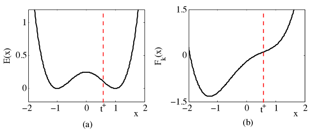
The modifications of the original dimer algorithms that we have in Algorithm 3 would, in the case of optimisation, yield a globally convergent scheme. Unfortunately, this is not the case in the saddle search case. To see this, consider a one-dimensional double-well example,

E(x)=14(1x2)2=14x412x2+14;𝐸𝑥14superscript1superscript𝑥2214superscript𝑥412superscript𝑥214E(x)={\textstyle\frac{1}{4}}(1-x^{2})^{2}={\textstyle\frac{1}{4}}x^{4}-{\textstyle\frac{1}{2}}x^{2}+{\textstyle\frac{1}{4}}; (16)

cf. Figure 1(a). There are only two possible (equivalent) dimer orientation v=±1𝑣plus-or-minus1v=\pm 1, and therefore the rotation steps in Algorithm 3 are ignored. We always take v=1𝑣1v=1 without loss of generality. The translation search direction at step k𝑘k is always given by p=(12)xh(xk,1)=xh(xk,1)𝑝12subscript𝑥subscriptsubscript𝑥𝑘1subscript𝑥subscriptsubscript𝑥𝑘1p=-(1-2)\nabla_{x}\mathcal{E}_{h}(x_{k},1)=\nabla_{x}\mathcal{E}_{h}(x_{k},1), i.e., an ascent direction.

Refer to caption
Figure 1. (a) Double-well energy defined in (16). (b) The auxiliary functional Fk(x)subscript𝐹𝑘𝑥F_{k}(x) with xk=th+subscript𝑥𝑘subscriptsuperscript𝑡x_{k}=t^{+}_{h}; cf. §3.3. The second turning point th=th+subscriptsuperscript𝑡subscriptsuperscript𝑡t^{-}_{h}=-t^{+}_{h} is an admissible descent step for Fksubscript𝐹𝑘F_{k}, hence the dimer method can potentially cycle.

It is easy to see that x=0subscript𝑥0x_{*}=0 is an index-1 saddle (i.e., a maximum), and that there are two turning points t±=±31/2superscript𝑡plus-or-minusplus-or-minussuperscript312t^{\pm}=\pm 3^{-1/2}. Thus, there exist “discrete turning points” th±=±31/2+O(h2)subscriptsuperscript𝑡plus-or-minusplus-or-minussuperscript312𝑂superscript2t^{\pm}_{h}=\pm 3^{-1/2}+O(h^{2}) such that λ(th±)=0𝜆subscriptsuperscript𝑡plus-or-minus0\lambda(t^{\pm}_{h})=0, where λ(x)=Hh(x;1)1=12h2(E(x+h)E(xh))𝜆𝑥subscript𝐻𝑥1112superscript2superscript𝐸𝑥superscript𝐸𝑥\lambda(x)=H_{h}(x;1)\cdot 1={\textstyle\frac{1}{2h^{2}}}(E^{\prime}(x+h)-E^{\prime}(x-h)).

Suppose that we have an iterate xk=th+subscript𝑥𝑘subscriptsuperscript𝑡x_{k}=t^{+}_{h}, then the translation search direction is p+=xh(th+,1)<0superscript𝑝subscript𝑥subscriptsubscriptsuperscript𝑡10p^{+}=\nabla_{x}\mathcal{E}_{h}(t^{+}_{h},1)<0. Since h(th)=h(th+)subscriptsubscriptsuperscript𝑡subscriptsubscriptsuperscript𝑡\mathcal{E}_{h}(t^{-}_{h})=\mathcal{E}_{h}(t^{+}_{h}) it follows that

Fk(th)=h(th)2p+(thth+)<h(th)=Fk(th+).subscript𝐹𝑘subscriptsuperscript𝑡subscriptsubscriptsuperscript𝑡2superscript𝑝subscriptsuperscript𝑡subscriptsuperscript𝑡subscriptsubscriptsuperscript𝑡subscript𝐹𝑘subscriptsuperscript𝑡F_{k}(t^{-}_{h})=\mathcal{E}_{h}(t^{-}_{h})-2p^{+}(t^{-}_{h}-t^{+}_{h})<\mathcal{E}_{h}(t^{-}_{h})=F_{k}(t^{+}_{h}).

Thus, for ΘΘ\Theta sufficiently small, the update xk+1=thsubscript𝑥𝑘1subscriptsuperscript𝑡x_{k+1}=t^{-}_{h} satisfies all the conditions for termination of the loop (11)–(12) in Algorithm 3. See also Figure 1 (b), where Fksubscript𝐹𝑘F_{k} is visualised.

We therefore conclude that our newly proposed variant of the dimer algorithm does not excluded cycling behaviour. We also remark that the example is not exclusively one-dimensional, but that analogous constructions can be readily made in any dimension.

3.4. Local convergence

We now establish a local convergence rate.


Theorem 7. Let (x,v,λ)subscript𝑥subscript𝑣subscript𝜆(x_{*},v_{*},\lambda_{*}) be an index-1 saddle, let (xh,vh,λh)subscript𝑥subscript𝑣subscript𝜆(x_{h},v_{h},\lambda_{h}) denote the dimer saddle associated with (x,v,λ)subscript𝑥subscript𝑣subscript𝜆(x_{*},v_{*},\lambda_{*}) (cf. Theorem 2.3) and let xk,vksubscript𝑥𝑘subscript𝑣𝑘x_{k},v_{k} be the iterates generated by the Linesearch Dimer Algorithm. Then there exist r,h0,C>0𝑟subscript0𝐶0r,h_{0},C>0 and γ(0,1)𝛾01\gamma\in(0,1) such that, for x0Br(x)subscript𝑥0subscript𝐵𝑟subscript𝑥x_{0}\in B_{r}(x_{*}), v1Br(v)SXsubscript𝑣1subscript𝐵𝑟subscript𝑣subscript𝑆𝑋v_{-1}\in B_{r}(v_{*})\cap S_{X} and hh0subscript0h\leq h_{0}, one of the following alternatives are true:

  • (i)

    If xh(xk,vk1)=0subscript𝑥subscriptsubscript𝑥𝑘subscript𝑣𝑘10\nabla_{x}\mathcal{E}_{h}(x_{k},v_{k-1})=0 for some k𝑘k\in\mathbb{N}, then xkxhCh2normsubscript𝑥𝑘subscript𝑥𝐶superscript2\|x_{k}-x_{h}\|\leq Ch^{2}.

  • (ii)

    If xh(xk,vk1)0subscript𝑥subscriptsubscript𝑥𝑘subscript𝑣𝑘10\nabla_{x}\mathcal{E}_{h}(x_{k},v_{k-1})\neq 0 for all k𝑘k\in\mathbb{N}, then

    xkxh+vkvhCγk(x0xh+h2v1vh),normsubscript𝑥𝑘subscript𝑥normsubscript𝑣𝑘subscript𝑣𝐶superscript𝛾𝑘normsubscript𝑥0subscript𝑥superscript2normsubscript𝑣1subscript𝑣\|x_{k}-x_{h}\|+\|v_{k}-v_{h}\|\leq C\gamma^{k}\big{(}\|x_{0}-x_{h}\|+h^{2}\|v_{-1}-v_{h}\|\big{)}, (17)
Sketch of proof.

Case (i) merely serves to exclude an unlikely situation, in which the Rotation algorithm is ill-defined. We do not discuss this case here, but treat it in §A.5.1. In the following assume Case (ii).

Let rk=xkxhsubscript𝑟𝑘normsubscript𝑥𝑘subscript𝑥r_{k}=\|x_{k}-x_{h}\| and sk:=vkvhassignsubscript𝑠𝑘normsubscript𝑣𝑘subscript𝑣s_{k}:=\|v_{k}-v_{h}\|.

0. We recall basic contraction results for Armijo-based linesearch methods both in a general Hilbert space and for iterates constrained to lie on the unit sphere in §A.4.

1. As a first proper step we establish that, under the termination criterion (1vkvk)Hh(xk;vk)xh(xk,vk1)norm1tensor-productsubscript𝑣𝑘subscript𝑣𝑘subscript𝐻subscript𝑥𝑘subscript𝑣𝑘normsubscript𝑥subscriptsubscript𝑥𝑘subscript𝑣𝑘1\|(1-v_{k}\otimes v_{k})H_{h}(x_{k};v_{k})\|\leq\|\nabla_{x}\mathcal{E}_{h}(x_{k},v_{k-1})\| for the rotation step, it follows that vkvhrk+h2sk1less-than-or-similar-tonormsubscript𝑣𝑘subscript𝑣subscript𝑟𝑘superscript2subscript𝑠𝑘1\|v_{k}-v_{h}\|\lesssim r_{k}+h^{2}s_{k-1}. This is proven in Lemma A.5 and Lemma A.5.

2. Next, we use this result to establish that there exists a local minimizer yksubscript𝑦𝑘y_{k} of Fksubscript𝐹𝑘F_{k} satisfying ykxhrk2+h2rk+h4sk1less-than-or-similar-tonormsubscript𝑦𝑘subscript𝑥superscriptsubscript𝑟𝑘2superscript2subscript𝑟𝑘superscript4subscript𝑠𝑘1\|y_{k}-x_{h}\|\lesssim r_{k}^{2}+h^{2}r_{k}+h^{4}s_{k-1}. This is established in Lemma A.5.

3. The linesearch procedure and the upper bound on the step length ensure that the step of xksubscript𝑥𝑘x_{k} to xk+1subscript𝑥𝑘1x_{k+1} contracts towards yksubscript𝑦𝑘y_{k}, that is, xk+1ykγxkyksubscriptnormsubscript𝑥𝑘1subscript𝑦𝑘subscript𝛾subscriptnormsubscript𝑥𝑘subscript𝑦𝑘\|x_{k+1}-y_{k}\|_{*}\leq\gamma_{*}\|x_{k}-y_{k}\|_{*} for some γ(0,1)subscript𝛾01\gamma_{*}\in(0,1) and \|\cdot\|_{*} the energy norm induced by (I2vv)2E(x)2Fk(yk)𝐼tensor-product2subscript𝑣subscript𝑣superscript2𝐸subscript𝑥superscript2subscript𝐹𝑘subscript𝑦𝑘(I-2v_{*}\otimes v_{*})\nabla^{2}E(x_{*})\approx\nabla^{2}F_{k}(y_{k}). This is obtained in Lemma A.5.

4. The three preceding steps can then be combined to establish that, for r0,s1,hsubscript𝑟0subscript𝑠1r_{0},s_{-1},h sufficiently small, there exists a constant γ3(γ,1)subscript𝛾3subscript𝛾1\gamma_{3}\in(\gamma_{*},1) such that

rk+1+h2skγ3(rk+h2sk1),superscriptsubscript𝑟𝑘1superscript2subscript𝑠𝑘subscript𝛾3superscriptsubscript𝑟𝑘superscript2subscript𝑠𝑘1r_{k+1}^{*}+h^{2}s_{k}\leq\gamma_{3}(r_{k}^{*}+h^{2}s_{k-1}),

where rk:=xkxhassignsuperscriptsubscript𝑟𝑘subscriptnormsubscript𝑥𝑘subscript𝑥r_{k}^{*}:=\|x_{k}-x_{h}\|_{*}. This contraction result readily implies the result of the theorem.

The complete proof is given in §A.5. ∎

4. Numerical Tests

4.1. Remarks on the implementation

Here, we remark on how preconditioning is implemented and on some further details of our implementation that slightly deviate from the theoretical formulations of Algorithms 1 and 3.

In all cases the underlying space is X=N𝑋superscript𝑁X=\mathbb{R}^{N} for some N𝑁N\in\mathbb{N}. The main deviation from Algorithms 1 and 3 is that we admit general Euclidean norms and inner products that may change from one step to another,

u=uTMku,anduv=uTMkv,formulae-sequencenorm𝑢superscript𝑢𝑇subscript𝑀𝑘𝑢and𝑢𝑣superscript𝑢𝑇subscript𝑀𝑘𝑣\|u\|=\sqrt{u^{T}M_{k}u},\qquad\text{and}\qquad u\cdot v=u^{T}M_{k}v,

where Mksubscript𝑀𝑘M_{k} is symmetric and positive definite. That is, our implementation is a variable metric variant.

Let EC4(X)=C4(N)𝐸superscript𝐶4𝑋superscript𝐶4superscript𝑁E\in C^{4}(X)=C^{4}(\mathbb{R}^{N}), and let superscript\nabla^{\prime} denote the standard gradient and superscripttensor-product\otimes^{\prime} the standard tensor product (i.e., the gradient and tensor products with respect to the 2superscript2\ell^{2}-norm), then the gradient and tensor products in step k𝑘k become

E(x)=Mk1E(x),and(vv)E(x)=(vv)E(x).formulae-sequence𝐸𝑥superscriptsubscript𝑀𝑘1superscript𝐸𝑥andtensor-product𝑣𝑣𝐸𝑥superscripttensor-product𝑣𝑣superscript𝐸𝑥\nabla E(x)=M_{k}^{-1}\nabla^{\prime}E(x),\quad\text{and}\quad(v\otimes v)\nabla E(x)=(v\otimes^{\prime}v)\nabla^{\prime}E(x).

The variable metric variant of Algorithm 1, augmented with a termination criterion, is given below. For the purposes of the numerical testing we call this the simple dimer method, it is effectively a forward Euler ODE integrator for the dimer dynamics. (Note also that here the rotation step is performed by a simple descent step followed by a projection, rather than a step on the manifold.)

Algorithm 1vmvm{}^{\mbox{\tiny vm}}:

  1. (1)

    Input: x0,v0Xsubscript𝑥0subscript𝑣0𝑋x_{0},v_{0}\in X, h>00h>0,α,β>0𝛼𝛽0\alpha,\beta>0,TOLx,TOLv>0superscriptTOL𝑥superscriptTOL𝑣0{\rm TOL}^{x},{\rm TOL}^{v}>0; k:=0assign𝑘0k:=0;

  2. (2)

    While Mk1/2xh(xk,vk)2>TOLxsubscriptnormsuperscriptsubscript𝑀𝑘12superscriptsubscript𝑥subscriptsubscript𝑥𝑘subscript𝑣𝑘superscript2superscriptTOL𝑥\|M_{k}^{-1/2}\nabla_{x}^{\prime}\mathcal{E}_{h}(x_{k},v_{k})\|_{\ell^{2}}>{\rm TOL}^{x}
    .                    or (Mk1/2Mk1/2vkvk)h2vh(xk,vk)2>TOLvsubscriptnormsuperscriptsubscript𝑀𝑘12superscripttensor-productsuperscriptsubscript𝑀𝑘12subscript𝑣𝑘subscript𝑣𝑘superscript2superscriptsubscript𝑣subscriptsubscript𝑥𝑘subscript𝑣𝑘superscript2superscriptTOL𝑣\|(M_{k}^{-1/2}-M_{k}^{1/2}v_{k}\otimes^{\prime}v_{k})h^{-2}\nabla_{v}^{\prime}\mathcal{E}_{h}(x_{k},v_{k})\|_{\ell^{2}}>{\rm TOL}^{v}    do

  3. %% Metric %%

  4. (3)

    Compute a spd matrix MkN×Nsubscript𝑀𝑘superscript𝑁𝑁M_{k}\in\mathbb{R}^{N\times N};

  5. (4)

    vk:=vk/Mk1/2vkassignsubscript𝑣𝑘subscript𝑣𝑘normsuperscriptsubscript𝑀𝑘12subscript𝑣𝑘v_{k}:=v_{k}/\|M_{k}^{1/2}v_{k}\|;

  6. (5)

    vk+1:=vkβ(Mk1vkvk)h2vh(xk,vk)assignsubscript𝑣𝑘1subscript𝑣𝑘𝛽superscriptsubscript𝑀𝑘1tensor-productsubscript𝑣𝑘subscript𝑣𝑘superscript2superscriptsubscript𝑣subscriptsubscript𝑥𝑘subscript𝑣𝑘v_{k+1}:=v_{k}-\beta(M_{k}^{-1}-v_{k}\otimes v_{k})h^{-2}\nabla_{v}^{\prime}\mathcal{E}_{h}(x_{k},v_{k})

  7. (6)

    xk+1:=xkα(Mk12vkvk)xh(xk,vk)assignsubscript𝑥𝑘1subscript𝑥𝑘𝛼superscriptsubscript𝑀𝑘1tensor-product2subscript𝑣𝑘subscript𝑣𝑘superscriptsubscript𝑥subscriptsubscript𝑥𝑘subscript𝑣𝑘x_{k+1}:=x_{k}-\alpha(M_{k}^{-1}-2v_{k}\otimes v_{k})\nabla_{x}^{\prime}\mathcal{E}_{h}(x_{k},v_{k}).

  8. (7)

    k:=k+1assign𝑘𝑘1k:=k+1

Remark 8. In our experiments we observe that the rotation residual decreases more quickly than the translation residual, hence the convergence criteria could be based on the translation residual only, without affecting the results. ∎


Remark 9. Our analysis of both the Simple Dimer Algorithm and of the Linesearch Dimer Algorithm is readily extended to their variable metric variants, provided that the metric Mksubscript𝑀𝑘M_{k} at iterate k𝑘k is a smooth function of the state, i.e., Mk=𝐌(xk,vk)subscript𝑀𝑘𝐌subscript𝑥𝑘subscript𝑣𝑘M_{k}={\bf M}(x_{k},v_{k}), where 𝐌C2(Br(x)×SX;L(X))𝐌superscript𝐶2subscript𝐵𝑟subscript𝑥subscript𝑆𝑋𝐿𝑋{\bf M}\in C^{2}(B_{r}(x_{*})\times S_{X};L(X)), for some r>0𝑟0r>0. This is the case in all examples that we consider below. A more general convergence theory, e.g., employing quasi-Newton type hessian updates requires additional work. ∎

Analogous modifications are made to Algorithm 3. The auxiliary functional Fksubscript𝐹𝑘F_{k} now reads

Fk(x)subscript𝐹𝑘𝑥\displaystyle F_{k}(x) =h(x;vk)2(vkTxh(xk,vk))(vkTMk(xxk))+λk(vkTMk(xxk))2,absentsubscript𝑥subscript𝑣𝑘2superscriptsubscript𝑣𝑘𝑇superscriptsubscript𝑥subscriptsubscript𝑥𝑘subscript𝑣𝑘superscriptsubscript𝑣𝑘𝑇subscript𝑀𝑘𝑥subscript𝑥𝑘subscript𝜆𝑘superscriptsuperscriptsubscript𝑣𝑘𝑇subscript𝑀𝑘𝑥subscript𝑥𝑘2\displaystyle=\mathcal{E}_{h}(x;v_{k})-2\big{(}v_{k}^{T}\nabla_{x}^{\prime}\mathcal{E}_{h}(x_{k},v_{k})\big{)}\big{(}v_{k}^{T}M_{k}(x-x_{k})\big{)}+\lambda_{k}\big{(}v_{k}^{T}M_{k}(x-x_{k})\big{)}^{2},
λksubscript𝜆𝑘\displaystyle\lambda_{k} =h2vkTvh(xk,vk),absentsuperscript2superscriptsubscript𝑣𝑘𝑇superscriptsubscript𝑣subscriptsubscript𝑥𝑘subscript𝑣𝑘\displaystyle=h^{-2}v_{k}^{T}\nabla_{v}^{\prime}\mathcal{E}_{h}(x_{k},v_{k}),
xh(x,v)superscriptsubscript𝑥subscript𝑥𝑣\displaystyle\nabla_{x}^{\prime}\mathcal{E}_{h}(x,v) =12(E(x+hv)+E(xhv)),absent12superscript𝐸𝑥𝑣superscript𝐸𝑥𝑣\displaystyle={\textstyle\frac{1}{2}}\big{(}\nabla^{\prime}E(x+hv)+\nabla^{\prime}E(x-hv)\big{)},
vh(x,v)superscriptsubscript𝑣subscript𝑥𝑣\displaystyle\nabla_{v}^{\prime}\mathcal{E}_{h}(x,v) =h2(E(x+hv)E(xhv)),absent2superscript𝐸𝑥𝑣superscript𝐸𝑥𝑣\displaystyle={\textstyle\frac{h}{2}}\big{(}\nabla^{\prime}E(x+hv)-\nabla^{\prime}E(x-hv)\big{)},

where we recall that superscript\nabla^{\prime} denotes the standard gradient (i.e., the gradient with respect to the 2superscript2\ell^{2}-norm).

Algorithm 3vmvm{}^{\mbox{\tiny vm}}:

  1. (1)

    Input: x0,v0Xsubscript𝑥0subscript𝑣0𝑋x_{0},v_{0}\in X, h>00h>0,TOLx,TOLv>0superscriptTOL𝑥superscriptTOL𝑣0{\rm TOL}^{x},{\rm TOL}^{v}>0; k:=0assign𝑘0k:=0;

  2. (2)

    While Mk1/2xh(xk,vk)2>TOLxsubscriptnormsuperscriptsubscript𝑀𝑘12superscriptsubscript𝑥subscriptsubscript𝑥𝑘subscript𝑣𝑘superscript2superscriptTOL𝑥\|M_{k}^{-1/2}\nabla_{x}^{\prime}\mathcal{E}_{h}(x_{k},v_{k})\|_{\ell^{2}}>{\rm TOL}^{x}

  3. %% Metric %%

  4. (3)

    Compute a spd matrix MkN×Nsubscript𝑀𝑘superscript𝑁𝑁M_{k}\in\mathbb{R}^{N\times N};

  5. (4)

    vk:=vk/Mk1/2vk1assignsuperscriptsubscript𝑣𝑘subscript𝑣𝑘normsuperscriptsubscript𝑀𝑘12subscript𝑣𝑘1v_{k}^{\prime}:=v_{k}/\|M_{k}^{1/2}v_{k-1}\|;

  6. %% Rotation %%

  7. (5)

    vk+1:=Rotation (VM)[xk,vk,β,Mk]assignsubscript𝑣𝑘1Rotation (VM)subscript𝑥𝑘superscriptsubscript𝑣𝑘𝛽subscript𝑀𝑘v_{k+1}:=\text{\bf Rotation (VM)}[x_{k},v_{k}^{\prime},\beta,M_{k}]

  8. %% Translation %%

  9. (6)

    pM:=(Mk12vk+1vk+1)xh(xk;vk+1)assignsubscript𝑝𝑀superscriptsubscript𝑀𝑘1tensor-product2subscript𝑣𝑘1subscript𝑣𝑘1superscriptsubscript𝑥subscriptsubscript𝑥𝑘subscript𝑣𝑘1p_{M}:=-(M_{k}^{-1}-2v_{k+1}\otimes v_{k+1})\nabla_{x}^{\prime}\mathcal{E}_{h}(x_{k};v_{k+1})

  10. (7)

    α:=min(αmax,2α)assign𝛼subscript𝛼max2𝛼\alpha:=\min(\alpha_{\rm max},2\alpha)

  11. (8)

    While (Fk(xk+αpM)>Fk(xk)ΘαpMTMkpMsubscript𝐹𝑘subscript𝑥𝑘𝛼subscript𝑝𝑀subscript𝐹𝑘subscript𝑥𝑘Θ𝛼superscriptsubscript𝑝𝑀𝑇subscript𝑀𝑘subscript𝑝𝑀F_{k}(x_{k}+\alpha p_{M})>F_{k}(x_{k})-\Theta\alpha p_{M}^{T}M_{k}p_{M})
    .             or (Mk1/2(Mk1vk+1vk+1)h2vh(xk+αpM;vk+1)2>subscriptnormsuperscriptsubscript𝑀𝑘12superscriptsubscript𝑀𝑘1tensor-productsubscript𝑣𝑘1subscript𝑣𝑘1superscript2superscriptsubscript𝑣subscriptsubscript𝑥𝑘𝛼subscript𝑝𝑀subscript𝑣𝑘1superscript2absent\|M_{k}^{1/2}(M_{k}^{-1}-v_{k+1}\otimes v_{k+1})h^{-2}\nabla_{v}^{\prime}\mathcal{E}_{h}(x_{k}+\alpha p_{M};v_{k+1})\|_{\ell^{2}}>
    .                   ΨMk1/2(Mk1vk+1vk+1)h2vh(xk;vk+1)2Ψsubscriptnormsuperscriptsubscript𝑀𝑘12superscriptsubscript𝑀𝑘1tensor-productsubscript𝑣𝑘1subscript𝑣𝑘1superscript2superscriptsubscript𝑣subscriptsubscript𝑥𝑘subscript𝑣𝑘1superscript2\Psi\|M_{k}^{1/2}(M_{k}^{-1}-v_{k+1}\otimes v_{k+1})h^{-2}\nabla_{v}^{\prime}\mathcal{E}_{h}(x_{k};v_{k+1})\|_{\ell^{2}}) do

  12. (9)

    α:=α/2assign𝛼𝛼2\alpha:=\alpha/2

  13. (10)

    xk+1:=xk+αpMassignsubscript𝑥𝑘1subscript𝑥𝑘𝛼subscript𝑝𝑀x_{k+1}:=x_{k}+\alpha p_{M}.

  14. (11)

    k:=k+1assign𝑘𝑘1k:=k+1

Rotationvmvm{}^{\mbox{\tiny vm}}:

  1. (1)

    Input: x,v,β,Mk𝑥𝑣𝛽subscript𝑀𝑘x,v,\beta,M_{k}
    Parameters: TOL=max(Mk1/2xh(x,v)2,TOLv{\rm TOL}=\max(\|M_{k}^{-1/2}\nabla_{x}^{\prime}\mathcal{E}_{h}(x,v)\|_{\ell^{2}},{\rm TOL}^{v}), Θ(0,1)Θ01\Theta\in(0,1), βmaxsubscript𝛽max\beta_{\rm max};

  2. (2)

    While Mk1/2(Mk1vv)h2vh(x;v)>TOLnormsuperscriptsubscript𝑀𝑘12superscriptsubscript𝑀𝑘1tensor-product𝑣𝑣superscript2superscriptsubscript𝑣subscript𝑥𝑣TOL\|M_{k}^{1/2}(M_{k}^{-1}-v\otimes v)h^{-2}\nabla_{v}^{\prime}\mathcal{E}_{h}(x;v)\|>{\rm TOL} do

  3. (3)

    s:=(Mk1vv)h2vh(x;v)assign𝑠superscriptsubscript𝑀𝑘1tensor-product𝑣𝑣superscript2superscriptsubscript𝑣subscript𝑥𝑣s:=-(M_{k}^{-1}-v\otimes v)h^{-2}\nabla_{v}^{\prime}\mathcal{E}_{h}(x;v)

  4. (4)

    t:=Mk1/2s2assign𝑡subscriptnormsuperscriptsubscript𝑀𝑘12𝑠superscript2t:=\|M_{k}^{1/2}s\|_{\ell^{2}}; β:=min(βmax,2β)assign𝛽subscript𝛽max2𝛽\beta:=\min(\beta_{\rm max},2\beta)

  5. (5)

    vβ:=cos(tβ)v+sin(tβ)t1sassignsubscript𝑣𝛽𝑡𝛽𝑣𝑡𝛽superscript𝑡1𝑠v_{\beta}:=\cos(t\beta)v+\sin(t\beta)t^{-1}s

  6. (6)

    While h(x,vβ)>h(x,v)Θβt2subscript𝑥subscript𝑣𝛽subscript𝑥𝑣Θ𝛽superscript𝑡2\mathcal{E}_{h}(x,v_{\beta})>\mathcal{E}_{h}(x,v)-\Theta\beta t^{2} do

  7. (7)

    β:=β/2assign𝛽𝛽2\beta:=\beta/2

  8. (8)

    v:=vβassign𝑣subscript𝑣𝛽v:=v_{\beta}

  9. (9)

    Output: v,β𝑣𝛽v,\beta


Remark 10. An additional (optional) modification that can give significant performance gains is to employ a different heuristic for the initial guess of α𝛼\alpha in Step (7) of Algorithm 3vmvm{}^{\mbox{\tiny vm}}: With pM,k:=(Mk12vkvk)xh(xk;vk)assignsubscript𝑝𝑀𝑘superscriptsubscript𝑀𝑘1tensor-product2subscript𝑣𝑘subscript𝑣𝑘superscriptsubscript𝑥subscriptsubscript𝑥𝑘subscript𝑣𝑘p_{M,k}:=-(M_{k}^{-1}-2v_{k}\otimes v_{k})\nabla_{x}^{\prime}\mathcal{E}_{h}(x_{k};v_{k}) and pI,k:=(I2vkvk)xh(xk,vk)assignsubscript𝑝𝐼𝑘𝐼tensor-product2subscript𝑣𝑘subscript𝑣𝑘superscriptsubscript𝑥subscriptsubscript𝑥𝑘subscript𝑣𝑘p_{I,k}:=-(I-2v_{k}\otimes v_{k})\nabla_{x}^{\prime}\mathcal{E}_{h}(x_{k},v_{k}) let, for k2𝑘2k\geq 2, γk:=(pM,k1pI,k1)/(pM,kpI,k)assignsubscript𝛾𝑘superscriptsubscript𝑝𝑀𝑘1subscript𝑝𝐼𝑘1superscriptsubscript𝑝𝑀𝑘subscript𝑝𝐼𝑘\gamma_{k}:=(p_{M,k-1}\cdot^{\prime}p_{I,k-1})/(p_{M,k}\cdot^{\prime}p_{I,k}), then for k2𝑘2k\geq 2 we replace Step (7) with

α:=min(avg(γmax(2,k4),,γk),2α,αmax)assign𝛼avgsubscript𝛾2𝑘4subscript𝛾𝑘2𝛼subscript𝛼max\alpha:=\min\big{(}\mathrm{avg}(\gamma_{\max(2,k-4)},\ldots,\gamma_{k}),2\alpha,\alpha_{\rm max})

An analogous modification can be made for the rotation algorithm. ∎

In all numerical tests we use the following parameters: h=103superscript103h=10^{-3}, Θ=0.1Θ0.1\Theta=\sqrt{0.1}, TOLx=105superscriptTOL𝑥superscript105{\rm TOL}^{x}=10^{-5}, TOLv=101superscriptTOL𝑣superscript101{\rm TOL}^{v}=10^{-1}, αmax=1subscript𝛼max1\alpha_{\rm max}=1 and Ψ=100Ψ100\Psi=100. We briefly discuss these choices:

  • hh should be small enough such that the dimer saddle is sufficiently close to the true saddle (with respect to the length scales of the given problem), while large enough that numerical robustness does not become a problem for the rotation. In all our tests, h=103superscript103h=10^{-3} was a good compromise.

  • ΘΘ\Theta should be sufficiently large (though, 1/2absent12\leq 1/2) to ensure that the linesearch method finds steps which give a large decrease in dimer energy. It is often chosen much smaller than our choice of Θ=0.1Θ0.1\Theta=\sqrt{0.1} to immediately accept steps that make some progress. Our experience is that, with preconditioned search direction, our more stringent choice gives better performance.

  • The choice of TOLxsuperscriptTOL𝑥{\rm TOL}^{x} simply controls the desired level of convergence to the dimer saddle.

  • The parameter TOLvsuperscriptTOL𝑣{\rm TOL}^{v} should be chosen as weakly as possible such that either algorithm converges to the saddle. In Algorithm 3vmvm{}^{\mbox{\tiny vm}} rotations are performed such that the rotation residual is at least as good as the translation residual until it moves below this value. Subsequent translations may increase the rotation residual such that further applications of the rotation algorithm are needed. In practise this means that the rotation algorithm is performed at every iteration of Algorithm 3’ for the first few steps, then only sporadically or not at all once the rotation residual reaches TOLvsuperscriptTOL𝑣{\rm TOL}^{v}. The use of this parameter then decreases the overall number of gradient evaluations needed to find the dimer saddle, by only performing the rotation as necessary.

  • The maximum step αmaxsubscript𝛼max\alpha_{\rm max} should principally be chosen such that the dimer cannot translate into non-physical regimes for the given problem.

  • The parameter ΨΨ\Psi should be chosen >1absent1>1 and restricts the translation step from moving the dimer to a point where it becomes too badly orientated. In our numerical tests this parameter is set sufficiently large that this termination criteria for the translation never occurs (the translation always terminates by finding a sufficient decrease in the auxiliary functional Fksubscript𝐹𝑘F_{k}).


Remark 11. We observe during numerical testing that the rotation component of the linesearch dimer is somewhat vulnerable to rounding error in the objective function E𝐸E. As the dimer becomes increasingly well orientated, E𝐸\nabla E becomes almost orthogonal to the dimer orientation and any small rotation may result in a zero change (to numerical precision) in the dimer energy. In the numerical examples presented in this section, this never occurs since we use a relatively high value for TOLvsuperscriptTOL𝑣{\rm TOL}^{v}, that is the rotation is only ever weakly converged. In our examples this is sufficient for the the dimer to converge to the saddle. If a stronger level of converge were required, another technique should be used to improve the rotation residual further, such as changing to a gradient based method or simply making fixed steps. ∎

4.2. Test 1: A simple 2D example

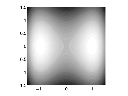
Our first example is taken from [28]. We equip X=2𝑋superscript2X=\mathbb{R}^{2} with the standard Euclidean inner product. The energy function is given by E(x,y)=(x21)2+y2𝐸𝑥𝑦superscriptsuperscript𝑥212superscript𝑦2E(x,y)=(x^{2}-1)^{2}+y^{2}, which has two simple symmetric minima at (±1,0)plus-or-minus10(\pm 1,0) and a unique index-1 saddle at (0,0)00(0,0). The energy function is given graphically in Figure 2.

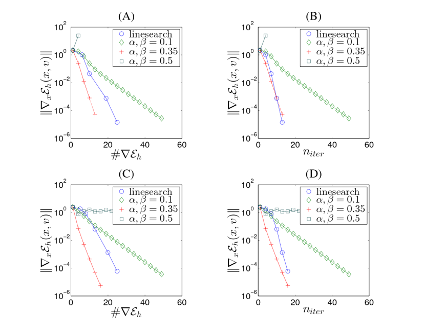
Figure 3 shows the x𝑥x-residual xh(x,v)normsubscript𝑥subscript𝑥𝑣\|\nabla_{x}\mathcal{E}_{h}(x,v)\| plotted against the number of function evaluations and the number of iterations.

The performance of the linesearch dimer is compared with a simple dimer method with different step sizes. Evidently a good choice of step is important. If a poor choice is made the algorithm may perform poorly or diverge. The linesearch dimer method requires a certain amount of overhead versus a simple dimer with well chosen step sizes. We can see in Figure 3 that the linesearch dimer may find a solution in fewer dimer iterations than the best fixed step tested (indicating that it found better steps), but using more gradient evaluations.
Refer to caption
Figure 2. Energy function for Test 1 with 2 symmetric minima and a unique index-1 saddle
Refer to caption
Figure 3. Convergence of the dimer to the saddle in a simple 2D example (Test 1).(A,B) The 2subscript2\ell_{2} norm of the x𝑥x gradient versus the number of force evaluations and the number of dimer iteration where the initial dimer state is x=[0.2,1],v=[1,1]formulae-sequence𝑥0.21𝑣11x=[0.2,1],v=[1,1]. In this case the choice α,β=0.5𝛼𝛽0.5\alpha,\beta=0.5 diverges immediately. (C,D) The 2subscript2\ell_{2} norm of the x𝑥x gradient versus the number of force evaluations and the number of dimer iterations where the initial dimer state is x=[0.2,1],v=[1,1]formulae-sequence𝑥0.21𝑣11x=[0.2,1],v=[1,1].

4.3. Test 2: Vacancy Diffusion

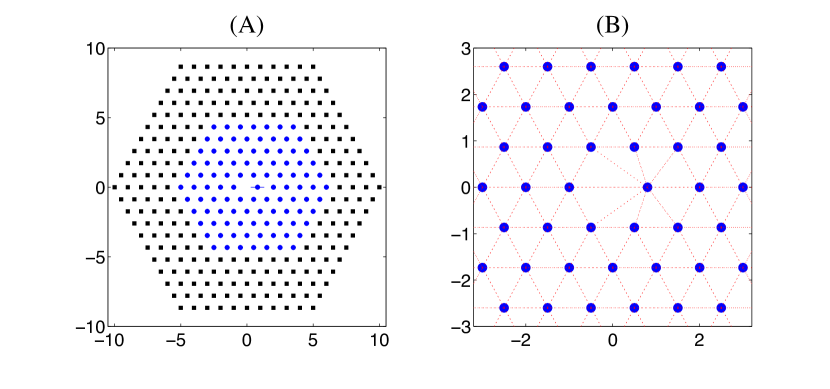
Our second test case is a standard example from molecular physics. A single atom is removed from a 2D lattice and a neighbouring atom is moved partway into the gap. Atoms within a certain radius of the vacancy are allowed to move, while those beyond that radius are fixed. This configuration is illustrated in Figure 4(A).

The energy function is given by the simple Morse potential,

E({xi})=i,jV(xixj2),V(r)=e2a(r1)2ea(r1),formulae-sequence𝐸subscript𝑥𝑖subscript𝑖𝑗𝑉subscriptnormsubscript𝑥𝑖subscript𝑥𝑗2𝑉𝑟superscript𝑒2𝑎𝑟12superscript𝑒𝑎𝑟1E(\{x_{i}\})=\sum_{i,j}V(\|x_{i}-x_{j}\|_{2}),\qquad V(r)=e^{-2a(r-1)}-2e^{-a(r-1)}, (18)

with stiffness parameter a=4𝑎4a=4.

Refer to caption
Figure 4. Initial configuration of the atoms in the vacancy diffusion problem (Test 2) . Black squares are fixed atoms while blue circles are atoms which move freely. (A) The initial dimer orientation is selected so that the translated atom has an orientation along the y=0𝑦0y=0 direction, and is zero for all other atoms. (B) The Delaunay 𝒯ksubscript𝒯𝑘\mathcal{T}_{k} triangulation used for the connectivity norm.

This test case demonstrates the importance of selecting the correct norm for high-dimensional problems. The experiment is run both using the generic 2subscript2\ell_{2} norm (no preconditioner), as well as a ‘connectivity’ norm. Such a norm can be defined based on the Delaunay triangulation of the atomistic positions (Figure 4(B))

Mku,u=|I𝒯ku|2,subscript𝑀𝑘𝑢𝑢superscriptsubscript𝐼subscript𝒯𝑘𝑢2\langle M_{k}u,u\rangle=\int|\nabla I_{\mathcal{T}_{k}}u|^{2},

where 𝒯ksubscript𝒯𝑘\mathcal{T}_{k} is the triangulation depicted in the figure and I𝒯ksubscript𝐼subscript𝒯𝑘I_{\mathcal{T}_{k}} the associated nodal interpolant.

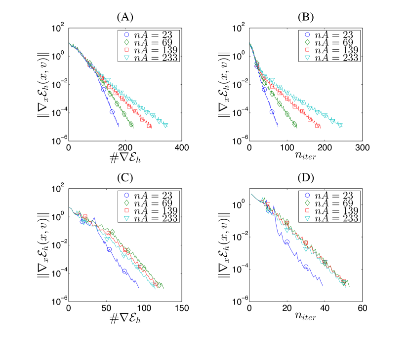
Figure 5 demonstrates the convergence to the saddle with different numbers of free atoms nA𝑛𝐴nA (giving different dimensionality of the system) in the two norms for the linesearch dimer.
Refer to caption
Figure 5. Convergence of the linesearch dimer to the saddle in the vacancy diffusion problem (Test 2) with (A),(C) the 2subscript2\ell_{2} norm and (B),(D) connectivity norm versus the number of force evaluations and dimer iterations for increasing numbers of free atoms.

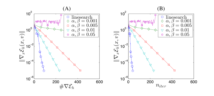
We can also observe the benefit of the linesearch vs a simple dimer scheme when using the connectivity norm (Figure 6). The linesearch dimer selects very efficient stepsizes with no a-priori information, while the simple dimer method might exhibit either slow convergence, or no convergence, if the fixed steps are poorly chosen.
Refer to caption
Figure 6. Convergence of the linesearch dimer vs the simple dimer method for Test 2 some choice of the of simple dimer step sizes with nA=69𝑛𝐴69nA=69 using the connectivity norm.

4.4. Test 3: A Phase Field Example

Our final example is based on a simple phase field model where the global energy is given by,

E(u)=Ωϵ2|u|2+12ϵ(u21)2.𝐸𝑢subscriptΩitalic-ϵ2superscript𝑢212italic-ϵsuperscriptsuperscript𝑢212E(u)=\int_{\Omega}\frac{\epsilon}{2}\left|\nabla u\right|^{2}+\frac{1}{2\epsilon}(u^{2}-1)^{2}. (19)

In our test ΩΩ\Omega is the unit square, and the boundary conditions are,

u(x)={1,x1{0,1}1,x2{0,1}.𝑢𝑥cases1subscript𝑥1011subscript𝑥201u(x)=\left\{\begin{array}[]{rl}-1,&x_{1}\in\{0,1\}\\ 1,&x_{2}\in\{0,1\}.\end{array}\right. (20)

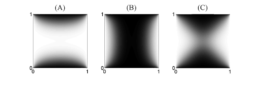
There are 2 minima of such an energy, these are given in Figure 7(A),(B). The saddle between these two minima is given in Figure 7(C).
Refer to caption
Figure 7. Minima (A,B) and saddle point (C) of the phase field problem (Test 3) with ϵ=1/10italic-ϵ110\epsilon=1/10. The shading is linearly interpolated between white(-1) and black(1).

A possible choice for a preconditioner for this system is a stabilized Laplacian,

P=ϵΔ+1ϵI.𝑃italic-ϵΔ1italic-ϵ𝐼P=\epsilon\Delta+\frac{1}{\epsilon}I. (21)

In order to compute either a minimum or a saddle point for such a system we triangulate the domain into a variable number of elements, thereby creating a discrete system of variable dimensionality. In our tests we take the initial dimer point as a small random perturbation of one of the local minima, and the initial dimer orientation is the metric inverted against a vector of ones.

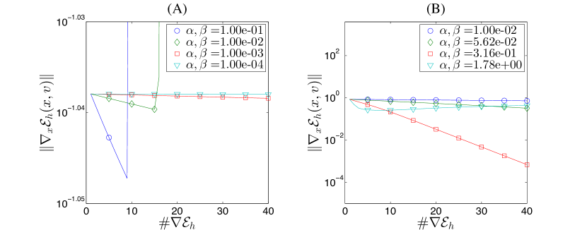
In Figure 8 we demonstrate the necessity of using a preconditioner to solve this problem using the simple dimer method. When using the preconditioner (21), the algorithm performs well when the step size is chosen appropriately. We observe the expected behaviour, that there exists an optimal step size where convergence is fastest, and beyond that step size the dimer diverges. In fact we observe that the stabilized Laplacian metric is so effective, that the optimal step size seems very close to the unit step. If the 2subscript2\ell_{2} norm (identity preconditioner) is used then for all step sizes tested the dimer diverges, indicating that at best a very small step would need to be chosen for convergence.
Refer to caption
Figure 8. Convergence of the simple dimer to the saddle in the phase field problem (Test 3) with (A) the 2subscript2\ell_{2} metric and (B) the stabilized Laplacian metric where ϵ=1/10italic-ϵ110\epsilon=1/10 for a triangulation with 3485 degrees of freedom.

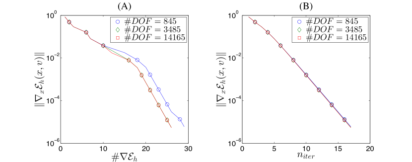
In Figure 9 we demonstrate that the used of the scaled Laplacian metric for different system sizes. We observe that the use of this metric gives almost perfect scale invariance.
Refer to caption
Figure 9. Convergence of the linesearch dimer to the saddle in the phase field problem (Test 3) with the stabilized Laplacian metric and triangulations of varying coarseness.

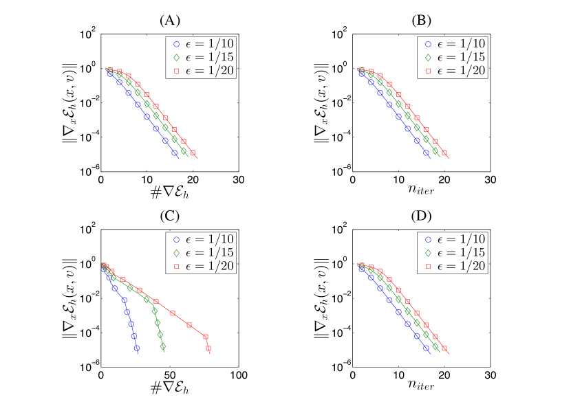
In Figure 10 we give the results of applying the simple and linesearch dimers with varying ϵitalic-ϵ\epsilon; the coarseness of the discretization in each experiment is chosen such that Δxϵ/5Δ𝑥italic-ϵ5\Delta x\approx\epsilon/5. In some of these cases the linesearch dimer fails due to rounding error. Specifically, due to rounding error in the naive implementation of the energy function (simple summation over the elements), the translation step fails to find a sufficient decrease in the dimer energy, the step size selected shrinks to zero (to rounding error) and the method stagnates. In order to correct this a more robust method of evaluating the energy or a more advanced optimization algorithm should be implemented which can either choose better linesearch directions or more robustly deal with numerically zero energy changes.

We also observe, in the case ϵ=1/30italic-ϵ130\epsilon=1/30 that the rate of convergence of even the simple dimer changes once the residual moves below a certain value. We are unable to give a satisfactory explanation for this effect, but speculate that the singularity in the boundary condition (which excludes admissible H1superscript𝐻1H^{1}-states) might be the case. (In particular, we observed that this behaviour is independent of the mesh coarseness and of the dimer length.)
Refer to caption
Figure 10. Convergence to the saddle in the phase field problem (Test 3) using the stabilized Laplacian metric with (A),(B) the simple dimer with unit step length and (C),(D) the linesearch dimer for a triangulation with 2405,9805,22205 degrees of freedom for the respective choices of ϵitalic-ϵ\epsilon.

5. Conclusions

We have described a dimer method for finding a saddle point in which the dimer length hh is not required to shrink to zero, but which converges to a point that lies within O(h2)𝑂superscript2O(h^{2}) of a saddle. We have enhanced this algorithm with a lineasearch to improve its robustness, and use the observation that the dimer method may be formulated and applied in a general Hilbert space to allow preconditioning that improves the method’s efficiency. The linesearch uses a local merit function. Unfortunately our particular merit function may not lead to global convergence of the iterates, and it is an open question as to whether there is another merit function that ensures global convergence. We have illustrated the positive effects of our algorithms on three realistic examples.

Appendix A Proofs

A.1. Proof of Proposition 2.3

We prove the result using the inverse function theorem. We write (9) as F(xh,vh,λh)=0𝐹subscript𝑥subscript𝑣subscript𝜆0F(x_{h},v_{h},\lambda_{h})=0 and show that F(x,v,λ)Ch2norm𝐹subscript𝑥subscript𝑣subscript𝜆𝐶superscript2\|F(x_{*},v_{*},\lambda_{*})\|\leq Ch^{2} and that F(x,v,λ)𝐹subscript𝑥subscript𝑣subscript𝜆\nabla F(x_{*},v_{*},\lambda_{*}) is an isomorphism with bounds independent of hh. The inverse function theorem then yields the stated result.

Residual estimate. Let the residual components be

rxsubscript𝑟𝑥\displaystyle r_{x} :=Fx(x,v,λ)=12(E(x+hv)+E(xhv)),assignabsentsubscript𝐹𝑥subscript𝑥subscript𝑣subscript𝜆12𝐸subscript𝑥subscript𝑣𝐸subscript𝑥subscript𝑣\displaystyle:=F_{x}(x_{*},v_{*},\lambda_{*})={\textstyle\frac{1}{2}}\big{(}\nabla E(x_{*}+hv_{*})+\nabla E(x_{*}-hv_{*})\big{)},
rvsubscript𝑟𝑣\displaystyle r_{v} :=Fv(x,v,λ)=12h(E(x+hv)E(xhv))λv,assignabsentsubscript𝐹𝑣subscript𝑥subscript𝑣subscript𝜆12𝐸subscript𝑥subscript𝑣𝐸subscript𝑥subscript𝑣subscript𝜆subscript𝑣\displaystyle:=F_{v}(x_{*},v_{*},\lambda_{*})={\textstyle\frac{1}{2h}}(\nabla E(x_{*}+hv_{*})-\nabla E(x_{*}-hv_{*}))-\lambda_{*}v_{*},
rλsubscript𝑟𝜆\displaystyle r_{\lambda} :=Fλ(x,v,λ)=12(v21).assignabsentsubscript𝐹𝜆subscript𝑥subscript𝑣subscript𝜆12superscriptnormsubscript𝑣21\displaystyle:=F_{\lambda}(x_{*},v_{*},\lambda_{*})={\textstyle\frac{1}{2}}(\|v_{*}\|^{2}-1).

Then,

rxsubscript𝑟𝑥\displaystyle r_{x} =E(x)+122E(x)(hvhv)+O(h2)=O(h2),absent𝐸subscript𝑥12superscript2𝐸subscript𝑥subscript𝑣subscript𝑣𝑂superscript2𝑂superscript2\displaystyle=\nabla E(x_{*})+{\textstyle\frac{1}{2}}\nabla^{2}E(x_{*})(hv_{*}-hv_{*})+O(h^{2})=O(h^{2}),
rvsubscript𝑟𝑣\displaystyle r_{v} =2E(x)vλv+1h(3E(x)[hvhvhvhv]+O(h2)=O(h2),\displaystyle=\nabla^{2}E(x_{*})v_{*}-\lambda_{*}v_{*}+{\textstyle\frac{1}{h}}\big{(}\nabla^{3}E(x_{*})[hv_{*}\otimes hv_{*}-hv_{*}\otimes hv_{*}]+O(h^{2})=O(h^{2}),
rλsubscript𝑟𝜆\displaystyle r_{\lambda} =0.absent0\displaystyle=0.

Thus, F(x,v,λ)Ch2norm𝐹subscript𝑥subscript𝑣subscript𝜆𝐶superscript2\|F(x_{*},v_{*},\lambda_{*})\|\leq Ch^{2}.

Stability. F(x,v,λ)𝐹subscript𝑥subscript𝑣subscript𝜆\nabla F(x_{*},v_{*},\lambda_{*}) can be written in the form

F(x,v,λ)𝐹subscript𝑥subscript𝑣subscript𝜆\displaystyle\nabla F(x_{*},v_{*},\lambda_{*}) =[2E(x+hv)+2E(xhv)2h2E(x+hv)2E(xhv)202E(x+hv)2E(xhv)2h2E(x+hv)+2E(xhv)2λIv0vT0]absentdelimited-[]matrixsuperscript2𝐸subscript𝑥subscript𝑣superscript2𝐸subscript𝑥subscript𝑣2superscript2𝐸subscript𝑥subscript𝑣superscript2𝐸subscript𝑥subscript𝑣20superscript2𝐸subscript𝑥subscript𝑣superscript2𝐸subscript𝑥subscript𝑣2superscript2𝐸subscript𝑥subscript𝑣superscript2𝐸subscript𝑥subscript𝑣2subscript𝜆𝐼subscript𝑣0superscriptsubscript𝑣𝑇0\displaystyle=\left[\begin{matrix}\frac{\nabla^{2}E(x_{*}+hv_{*})+\nabla^{2}E(x_{*}-hv_{*})}{2}&h\frac{\nabla^{2}E(x_{*}+hv_{*})-\nabla^{2}E(x_{*}-hv_{*})}{2}&0\\ \frac{\nabla^{2}E(x_{*}+hv_{*})-\nabla^{2}E(x_{*}-hv_{*})}{2h}&\frac{\nabla^{2}E(x_{*}+hv_{*})+\nabla^{2}E(x_{*}-hv_{*})}{2}-\lambda_{*}I&v_{*}\\ 0&v_{*}^{T}&0\end{matrix}\right]
=[2E(x)003E(x)v2E(x)λIv0vT0]+O(h2)=:𝐀+O(h2).\displaystyle=\left[\begin{matrix}\nabla^{2}E(x_{*})&0&0\\ \nabla^{3}E(x_{*})\cdot v_{*}&\nabla^{2}E(x_{*})-\lambda_{*}I&v_{*}\\ 0&v_{*}^{T}&0\end{matrix}\right]+O(h^{2})=:{\bf A}+O(h^{2}).

where we used (3), (4) and (6). By assumption, 2E(x)superscript2𝐸subscript𝑥\nabla^{2}E(x_{*}) is an isomorphism on X𝑋X. Since, also by assumption, λsubscript𝜆\lambda_{*} is a simple eigenvalue, the block

[2E(x)λIvvT0]delimited-[]matrixsuperscript2𝐸subscript𝑥subscript𝜆𝐼subscript𝑣superscriptsubscript𝑣𝑇0\left[\begin{matrix}\nabla^{2}E(x_{*})-\lambda_{*}I&v_{*}\\ v_{*}^{T}&0\end{matrix}\right] (22)

is an isomorphism on X×𝑋X\times\mathbb{R} as well. Thus, 𝐀𝐀{\bf A} is an isomorphism on X×X×𝑋𝑋X\times X\times\mathbb{R} and consequently, for all hh sufficiently small, F(x,v,λ)=A+O(h2)𝐹subscript𝑥subscript𝑣subscript𝜆𝐴𝑂superscript2\nabla F(x_{*},v_{*},\lambda_{*})=A+O(h^{2}) is also an isomorphism, with a uniform bound on its inverse.

Thus, the inverse function theorem shows that there exist a radius r0>0subscript𝑟00r_{0}>0 and a dimer length h0>0subscript00h_{0}>0, such that, for hh0subscript0h\leq h_{0}, there exists a unique solution (xh,vh,λh)subscript𝑥subscript𝑣subscript𝜆(x_{h},v_{h},\lambda_{h}) to (9) in a ball of radius r0subscript𝑟0r_{0} about (x,v,λ)subscript𝑥subscript𝑣subscript𝜆(x_{*},v_{*},\lambda_{*}), satisfying the estimate (10).

A.2. Proof of Theorem 2.4 (a)

Fix r𝑟r and h0subscript0h_{0} sufficiently small so that Theorem 2.3 applies. Let ek:=xkxh,fk:=vkvhformulae-sequenceassignsubscript𝑒𝑘subscript𝑥𝑘subscript𝑥assignsubscript𝑓𝑘subscript𝑣𝑘subscript𝑣e_{k}:=x_{k}-x_{h},f_{k}:=v_{k}-v_{h} and rk:=ek2+fk2assignsubscript𝑟𝑘superscriptnormsubscript𝑒𝑘2superscriptnormsubscript𝑓𝑘2r_{k}:=\sqrt{\|e_{k}\|^{2}+\|f_{k}\|^{2}}, so that trivially ekrknormsubscript𝑒𝑘subscript𝑟𝑘\|e_{k}\|\leq r_{k} and fkrknormsubscript𝑓𝑘subscript𝑟𝑘\|f_{k}\|\leq r_{k}.


Lemma 12. Let p:=(I2vkvk)x(xk,vk)assign𝑝𝐼tensor-product2subscript𝑣𝑘subscript𝑣𝑘subscript𝑥subscript𝑥𝑘subscript𝑣𝑘p:=-(I-2v_{k}\otimes v_{k})\nabla_{x}\mathcal{E}(x_{k},v_{k}) and s:=(Ivkvk)Hh(xk;vk)assign𝑠𝐼tensor-productsubscript𝑣𝑘subscript𝑣𝑘subscript𝐻subscript𝑥𝑘subscript𝑣𝑘s:=-(I-v_{k}\otimes v_{k})H_{h}(x_{k};v_{k}), then, under the assumptions of Theorem 2.4,

p𝑝\displaystyle p =Aek+O(rk2+h2rk),andabsent𝐴subscript𝑒𝑘𝑂superscriptsubscript𝑟𝑘2superscript2subscript𝑟𝑘and\displaystyle=-Ae_{k}+O(r_{k}^{2}+h^{2}r_{k}),\qquad\text{and} (23)
s𝑠\displaystyle s =BekCfk+O(rk2+h2rk),absent𝐵subscript𝑒𝑘𝐶subscript𝑓𝑘𝑂superscriptsubscript𝑟𝑘2superscript2subscript𝑟𝑘\displaystyle=-Be_{k}-Cf_{k}+O(r_{k}^{2}+h^{2}r_{k}), (24)

where the operators A𝐴A and C𝐶C are defined in (14) and B𝐵B is a bounded linear operator.

Proof.

To prove (23) we first note the following identities which are easy to establish:

xh(x,v)subscript𝑥subscript𝑥𝑣\displaystyle\nabla_{x}\mathcal{E}_{h}(x,v) =E(x)+O(h2),absent𝐸𝑥𝑂superscript2\displaystyle=\nabla E(x)+O(h^{2}),
xh(xk,vk)xh(xh,vh)subscript𝑥subscriptsubscript𝑥𝑘subscript𝑣𝑘subscript𝑥subscriptsubscript𝑥subscript𝑣\displaystyle\nabla_{x}\mathcal{E}_{h}(x_{k},v_{k})-\nabla_{x}\mathcal{E}_{h}(x_{h},v_{h}) =O(rk),absent𝑂subscript𝑟𝑘\displaystyle=O(r_{k}),
vkvkvhvhtensor-productsubscript𝑣𝑘subscript𝑣𝑘tensor-productsubscript𝑣subscript𝑣\displaystyle v_{k}\otimes v_{k}-v_{h}\otimes v_{h} =O(rk),absent𝑂subscript𝑟𝑘\displaystyle=O(r_{k}),
x2h(xh,vh)superscriptsubscript𝑥2subscriptsubscript𝑥subscript𝑣\displaystyle\nabla_{x}^{2}\mathcal{E}_{h}(x_{h},v_{h}) =2E(xh)+O(h2)=2E(x)+O(h2)absentsuperscript2𝐸subscript𝑥𝑂superscript2superscript2𝐸subscript𝑥𝑂superscript2\displaystyle=\nabla^{2}E(x_{h})+O(h^{2})=\nabla^{2}E(x_{*})+O(h^{2})
xvh(xh,vh)subscript𝑥subscript𝑣subscriptsubscript𝑥subscript𝑣\displaystyle\nabla_{x}\nabla_{v}\mathcal{E}_{h}(x_{h},v_{h}) =12(2E(xh+hvh)2E(xhhvh))=O(h2).absent12superscript2𝐸subscript𝑥subscript𝑣superscript2𝐸subscript𝑥subscript𝑣𝑂superscript2\displaystyle={\textstyle\frac{1}{2}}\big{(}\nabla^{2}E(x_{h}+hv_{h})-\nabla^{2}E(x_{h}-hv_{h})\big{)}=O(h^{2}). (25)

Using these identities, we can expand

p𝑝\displaystyle p =(I2vkvk)(xh(xk,vk)xh(xh,vh)),absent𝐼tensor-product2subscript𝑣𝑘subscript𝑣𝑘subscript𝑥subscriptsubscript𝑥𝑘subscript𝑣𝑘subscript𝑥subscriptsubscript𝑥subscript𝑣\displaystyle=-(I-2v_{k}\otimes v_{k})\big{(}\nabla_{x}\mathcal{E}_{h}(x_{k},v_{k})-\nabla_{x}\mathcal{E}_{h}(x_{h},v_{h})\big{)},
=(I2vhvh)(x2h(xh,vh)ek+xvh(xh,vh)fk)+O(rk2)absent𝐼tensor-product2subscript𝑣subscript𝑣superscriptsubscript𝑥2subscriptsubscript𝑥subscript𝑣subscript𝑒𝑘subscript𝑥subscript𝑣subscriptsubscript𝑥subscript𝑣subscript𝑓𝑘𝑂superscriptsubscript𝑟𝑘2\displaystyle=-(I-2v_{h}\otimes v_{h})\big{(}\nabla_{x}^{2}\mathcal{E}_{h}(x_{h},v_{h})e_{k}+\nabla_{x}\nabla_{v}\mathcal{E}_{h}(x_{h},v_{h})f_{k}\big{)}+O(r_{k}^{2})
=(I2vhvh)2E(xh)ek+O(rk2+h2rk)absent𝐼tensor-product2subscript𝑣subscript𝑣superscript2𝐸subscript𝑥subscript𝑒𝑘𝑂superscriptsubscript𝑟𝑘2superscript2subscript𝑟𝑘\displaystyle=-(I-2v_{h}\otimes v_{h})\nabla^{2}E(x_{h})e_{k}+O(r_{k}^{2}+h^{2}r_{k})
=(I2vv)2E(x)ek+O(rk2+h2rk)absent𝐼tensor-product2subscript𝑣subscript𝑣superscript2𝐸subscript𝑥subscript𝑒𝑘𝑂superscriptsubscript𝑟𝑘2superscript2subscript𝑟𝑘\displaystyle=-(I-2v_{*}\otimes v_{*})\nabla^{2}E(x_{*})e_{k}+O(r_{k}^{2}+h^{2}r_{k})
=Aek+O(rk2+h2rk).absent𝐴subscript𝑒𝑘𝑂superscriptsubscript𝑟𝑘2superscript2subscript𝑟𝑘\displaystyle=-Ae_{k}+O(r_{k}^{2}+h^{2}r_{k}).

To prove (24), we first note that, with v=1norm𝑣1\|v\|=1,

Hh(x;v)subscript𝐻𝑥𝑣\displaystyle H_{h}(x;v) =112E(x+thv)dtv=2E(x)v+O(h2),absentsuperscriptsubscript11superscript2𝐸𝑥𝑡𝑣differential-d𝑡𝑣superscript2𝐸𝑥𝑣𝑂superscript2\displaystyle=\mathchoice{{\vbox{\hbox{$\textstyle-$ }}\kern-7.83337pt}}{{\vbox{\hbox{$\scriptstyle-$ }}\kern-5.90005pt}}{{\vbox{\hbox{$\scriptscriptstyle-$ }}\kern-4.75003pt}}{{\vbox{\hbox{$\scriptscriptstyle-$ }}\kern-4.25003pt}}\!\int_{-1}^{1}\nabla^{2}E(x+thv)\,{\rm d}t\,v=\nabla^{2}E(x)v+O(h^{2}),
Hh(xh;vh)subscript𝐻subscript𝑥subscript𝑣\displaystyle H_{h}(x_{h};v_{h}) =2E(xh)vh+O(h2)=2E(x)v+O(h2),absentsuperscript2𝐸subscript𝑥subscript𝑣𝑂superscript2superscript2𝐸subscript𝑥subscript𝑣𝑂superscript2\displaystyle=\nabla^{2}E(x_{h})v_{h}+O(h^{2})=\nabla^{2}E(x_{*})v_{*}+O(h^{2}),
Hh(xk;vk)Hh(xh;vh)subscript𝐻subscript𝑥𝑘subscript𝑣𝑘subscript𝐻subscript𝑥subscript𝑣\displaystyle H_{h}(x_{k};v_{k})-H_{h}(x_{h};v_{h}) =11(2E(xk+thvk)2E(xh+thvh))dtvkabsentsuperscriptsubscript11superscript2𝐸subscript𝑥𝑘𝑡subscript𝑣𝑘superscript2𝐸subscript𝑥𝑡subscript𝑣differential-d𝑡subscript𝑣𝑘\displaystyle=\mathchoice{{\vbox{\hbox{$\textstyle-$ }}\kern-7.83337pt}}{{\vbox{\hbox{$\scriptstyle-$ }}\kern-5.90005pt}}{{\vbox{\hbox{$\scriptscriptstyle-$ }}\kern-4.75003pt}}{{\vbox{\hbox{$\scriptscriptstyle-$ }}\kern-4.25003pt}}\!\int_{-1}^{1}\Big{(}\nabla^{2}E(x_{k}+thv_{k})-\nabla^{2}E(x_{h}+thv_{h})\Big{)}\,{\rm d}t\,v_{k}
+112E(xh+thvh)dt(vkvh)\displaystyle\qquad\qquad+\mathchoice{{\vbox{\hbox{$\textstyle-$ }}\kern-7.83337pt}}{{\vbox{\hbox{$\scriptstyle-$ }}\kern-5.90005pt}}{{\vbox{\hbox{$\scriptscriptstyle-$ }}\kern-4.75003pt}}{{\vbox{\hbox{$\scriptscriptstyle-$ }}\kern-4.25003pt}}\!\int_{-1}^{1}\nabla^{2}E(x_{h}+thv_{h})\,{\rm d}t(v_{k}-v_{h})
=11(3E(xh+thvh)[(xkxh)+th(vkvh)]dtvh\displaystyle=\mathchoice{{\vbox{\hbox{$\textstyle-$ }}\kern-7.83337pt}}{{\vbox{\hbox{$\scriptstyle-$ }}\kern-5.90005pt}}{{\vbox{\hbox{$\scriptscriptstyle-$ }}\kern-4.75003pt}}{{\vbox{\hbox{$\scriptscriptstyle-$ }}\kern-4.25003pt}}\!\int_{-1}^{1}\Big{(}\nabla^{3}E(x_{h}+thv_{h})\big{[}(x_{k}-x_{h})+th(v_{k}-v_{h})\big{]}\,{\rm d}tv_{h}
+2E(x)(vkvh)+O(rk2+h2rk)superscript2𝐸subscript𝑥subscript𝑣𝑘subscript𝑣𝑂superscriptsubscript𝑟𝑘2superscript2subscript𝑟𝑘\displaystyle\qquad\qquad+\nabla^{2}E(x_{*})(v_{k}-v_{h})+O(r_{k}^{2}+h^{2}r_{k})
=(3E(x)v)ek+2E(x)fk+O(h2rk+rk2),absentsuperscript3𝐸subscript𝑥subscript𝑣subscript𝑒𝑘superscript2𝐸subscript𝑥subscript𝑓𝑘𝑂superscript2subscript𝑟𝑘superscriptsubscript𝑟𝑘2\displaystyle=(\nabla^{3}E(x_{*})v_{*})e_{k}+\nabla^{2}E(x_{*})f_{k}+O(h^{2}r_{k}+r_{k}^{2}),

where we interpret 3E(x)vL(X)superscript3𝐸𝑥𝑣𝐿𝑋\nabla^{3}E(x)\cdot v\in L(X) via the action w((3E(x)v)z)=limt0t1w((2E(x+tv)2E(x))z)𝑤superscript3𝐸𝑥𝑣𝑧subscript𝑡0superscript𝑡1𝑤superscript2𝐸𝑥𝑡𝑣superscript2𝐸𝑥𝑧w\cdot((\nabla^{3}E(x)\cdot v)z)=\lim_{t\to 0}t^{-1}w\cdot((\nabla^{2}E(x+tv)-\nabla^{2}E(x))z). Finally, we also have

(vkvkvhvh)Hh(xh;vh)tensor-productsubscript𝑣𝑘subscript𝑣𝑘tensor-productsubscript𝑣subscript𝑣subscript𝐻subscript𝑥subscript𝑣\displaystyle(v_{k}\otimes v_{k}-v_{h}\otimes v_{h})H_{h}(x_{h};v_{h}) =(vkvkvhvh)2E(x)v+O(h2rk)absenttensor-productsubscript𝑣𝑘subscript𝑣𝑘tensor-productsubscript𝑣subscript𝑣superscript2𝐸subscript𝑥subscript𝑣𝑂superscript2subscript𝑟𝑘\displaystyle=(v_{k}\otimes v_{k}-v_{h}\otimes v_{h})\nabla^{2}E(x_{*})v_{*}+O(h^{2}r_{k})
=λ(vkvkvhvh)v+O(h2rk)absentsubscript𝜆tensor-productsubscript𝑣𝑘subscript𝑣𝑘tensor-productsubscript𝑣subscript𝑣subscript𝑣𝑂superscript2subscript𝑟𝑘\displaystyle=\lambda_{*}(v_{k}\otimes v_{k}-v_{h}\otimes v_{h})v_{*}+O(h^{2}r_{k})
=λ(vkvkvhvh)vh+O(h2rk)absentsubscript𝜆tensor-productsubscript𝑣𝑘subscript𝑣𝑘tensor-productsubscript𝑣subscript𝑣subscript𝑣𝑂superscript2subscript𝑟𝑘\displaystyle=\lambda_{*}(v_{k}\otimes v_{k}-v_{h}\otimes v_{h})v_{h}+O(h^{2}r_{k})
=λ(vkvh)+λvk((vkvh)vh)+O(h2rk)absentsubscript𝜆subscript𝑣𝑘subscript𝑣subscript𝜆subscript𝑣𝑘subscript𝑣𝑘subscript𝑣subscript𝑣𝑂superscript2subscript𝑟𝑘\displaystyle=\lambda_{*}(v_{k}-v_{h})+\lambda_{*}v_{k}((v_{k}-v_{h})\cdot v_{h})+O(h^{2}r_{k})
=λfk+O(rk2+h2rk).absentsubscript𝜆subscript𝑓𝑘𝑂superscriptsubscript𝑟𝑘2superscript2subscript𝑟𝑘\displaystyle=\lambda_{*}f_{k}+O(r_{k}^{2}+h^{2}r_{k}).

In the very last line we also used the fact that vkvh1=12vkvh2subscript𝑣𝑘subscript𝑣112superscriptnormsubscript𝑣𝑘subscript𝑣2v_{k}\cdot v_{h}-1={\textstyle\frac{1}{2}}\|v_{k}-v_{h}\|^{2}.

Using these identities, we can compute

s𝑠\displaystyle s =(Ivkvk)Hh(xk;vk)absent𝐼tensor-productsubscript𝑣𝑘subscript𝑣𝑘subscript𝐻subscript𝑥𝑘subscript𝑣𝑘\displaystyle=-(I-v_{k}\otimes v_{k})H_{h}(x_{k};v_{k})
=(Ivhvh)Hh(xh;vh)(Ivkvk)Hh(xk;vk)absent𝐼tensor-productsubscript𝑣subscript𝑣subscript𝐻subscript𝑥subscript𝑣𝐼tensor-productsubscript𝑣𝑘subscript𝑣𝑘subscript𝐻subscript𝑥𝑘subscript𝑣𝑘\displaystyle=(I-v_{h}\otimes v_{h})H_{h}(x_{h};v_{h})-(I-v_{k}\otimes v_{k})H_{h}(x_{k};v_{k})
=(Ivkvk)(Hh(xk;vk)Hh(xh;vh))+(vkvkvhvh)Hh(xh;vh)absent𝐼tensor-productsubscript𝑣𝑘subscript𝑣𝑘subscript𝐻subscript𝑥𝑘subscript𝑣𝑘subscript𝐻subscript𝑥subscript𝑣tensor-productsubscript𝑣𝑘subscript𝑣𝑘tensor-productsubscript𝑣subscript𝑣subscript𝐻subscript𝑥subscript𝑣\displaystyle=-(I-v_{k}\otimes v_{k})\big{(}H_{h}(x_{k};v_{k})-H_{h}(x_{h};v_{h})\big{)}+(v_{k}\otimes v_{k}-v_{h}\otimes v_{h})H_{h}(x_{h};v_{h})
=(Ivkvk)((3E(x)v)ek+2E(x)fk)+O(h2rk+rk2)absent𝐼tensor-productsubscript𝑣𝑘subscript𝑣𝑘superscript3𝐸subscript𝑥subscript𝑣subscript𝑒𝑘superscript2𝐸subscript𝑥subscript𝑓𝑘𝑂superscript2subscript𝑟𝑘superscriptsubscript𝑟𝑘2\displaystyle=-(I-v_{k}\otimes v_{k})\big{(}(\nabla^{3}E(x_{*})v_{*})e_{k}+\nabla^{2}E(x_{*})f_{k}\big{)}+O(h^{2}r_{k}+r_{k}^{2})
+λfk+O(rk2+h2rk)subscript𝜆subscript𝑓𝑘𝑂superscriptsubscript𝑟𝑘2superscript2subscript𝑟𝑘\displaystyle\qquad\qquad+\lambda_{*}f_{k}+O(r_{k}^{2}+h^{2}r_{k})
=:Bek+[λI(Ivv)2E(x)]fk+O(rk2+h2rk)\displaystyle=:-Be_{k}+\big{[}\lambda_{*}I-(I-v_{*}\otimes v_{*})\nabla^{2}E(x_{*})\big{]}f_{k}+O(r_{k}^{2}+h^{2}r_{k})
=BekCfk+O(rk2+h2rk).absent𝐵subscript𝑒𝑘𝐶subscript𝑓𝑘𝑂superscriptsubscript𝑟𝑘2superscript2subscript𝑟𝑘\displaystyle=-Be_{k}-Cf_{k}+O(r_{k}^{2}+h^{2}r_{k}).\qed

From Lemma A.2 it follows in particular that s=O(rk)𝑠𝑂subscript𝑟𝑘s=O(r_{k}). Hence, Taylor expansions of sine and cosine in the identity

vk+1=cos(sβk)vk+sin(sβk)ss,subscript𝑣𝑘1norm𝑠subscript𝛽𝑘subscript𝑣𝑘norm𝑠subscript𝛽𝑘𝑠norm𝑠v_{k+1}=\cos\big{(}\|s\|\beta_{k})v_{k}+\sin(\|s\|\beta_{k}){\textstyle\frac{s}{\|s\|}},

yield

fk+1=fk+βks+O(βk2sk2)subscript𝑓𝑘1subscript𝑓𝑘subscript𝛽𝑘𝑠𝑂superscriptsubscript𝛽𝑘2superscriptsubscript𝑠𝑘2f_{k+1}=f_{k}+\beta_{k}s+O(\beta_{k}^{2}s_{k}^{2})

Using Lemma A.2, the identity ek+1=ek+αkpsubscript𝑒𝑘1subscript𝑒𝑘subscript𝛼𝑘𝑝e_{k+1}=e_{k}+\alpha_{k}p, and the fact that βksubscript𝛽𝑘\beta_{k} is bounded, we therefore obtain identity (13) in the proof outline.

Upon defining

𝐀k:=(αkA0βkBβkC)and𝐞k=(ekfk)formulae-sequenceassignsubscript𝐀𝑘matrixsubscript𝛼𝑘𝐴0subscript𝛽𝑘𝐵subscript𝛽𝑘𝐶andsubscript𝐞𝑘matrixsubscript𝑒𝑘subscript𝑓𝑘{\bf A}_{k}:=\left(\begin{matrix}\alpha_{k}A&0\\ \beta_{k}B&\beta_{k}C\end{matrix}\right)\quad\text{and}\quad{\bf e}_{k}=\left(\begin{matrix}e_{k}\\ f_{k}\end{matrix}\right)

(13) reads

𝐞k+1=(I𝐀k)𝐞k+𝐭k,subscript𝐞𝑘1𝐼subscript𝐀𝑘subscript𝐞𝑘subscript𝐭𝑘{\bf e}_{k+1}=(I-{\bf A}_{k}){\bf e}_{k}+{\bf t}_{k}, (26)

where

𝐭kCt(αk+βk)(h2+rk)rk.normsubscript𝐭𝑘subscript𝐶tsubscript𝛼𝑘subscript𝛽𝑘superscript2subscript𝑟𝑘subscript𝑟𝑘\|{\bf t}_{k}\|\leq C_{\rm t}(\alpha_{k}+\beta_{k})(h^{2}+r_{k})r_{k}.

Due to the fact that A𝐴A is symmetric and positive definite, it follows that, for α¯,β¯¯𝛼¯𝛽\bar{\alpha},\bar{\beta} chosen sufficiently small and α¯=infkαk,β¯=infkβk>0formulae-sequence¯𝛼subscriptinfimum𝑘subscript𝛼𝑘¯𝛽subscriptinfimum𝑘subscript𝛽𝑘0\underline{\alpha}=\inf_{k}\alpha_{k},\underline{\beta}=\inf_{k}\beta_{k}>0, the spectrum of I𝐀k𝐼subscript𝐀𝑘I-{\bf A}_{k} is real and belongs to [0,1ϵ]01italic-ϵ[0,1-\epsilon] for some ϵ>0italic-ϵ0\epsilon>0, that depends on α¯,β¯¯𝛼¯𝛽\underline{\alpha},\underline{\beta}. This will be crucial later in the proof.


Lemma 13. Let 𝐏n,k:=i=nk(I𝐀i)assignsubscript𝐏𝑛𝑘superscriptsubscriptproduct𝑖𝑛𝑘𝐼subscript𝐀𝑖{\bf P}_{n,k}:=\prod_{i=n}^{k}(I-{\bf A}_{i}), for 0nk0𝑛𝑘0\leq n\leq k, then there exist constants C1>1,μ(0,1)formulae-sequencesubscript𝐶11𝜇01C_{1}>1,\mu\in(0,1) such that

𝐏n,kC1μkn+1.normsubscript𝐏𝑛𝑘subscript𝐶1superscript𝜇𝑘𝑛1\|{\bf P}_{n,k}\|\leq C_{1}\mu^{k-n+1}. (27)
Proof.

We assume, without loss of generality, that n=0𝑛0n=0. First, we note that the diagonal blocks

Ak:=[𝐏0,k]xx=i=0k(IαkA),andCk:=[𝐏0,k]vv=i=0k(IβkC),formulae-sequenceassignsubscript𝐴𝑘subscriptdelimited-[]subscript𝐏0𝑘𝑥𝑥superscriptsubscriptproduct𝑖0𝑘𝐼subscript𝛼𝑘𝐴assignandsubscript𝐶𝑘subscriptdelimited-[]subscript𝐏0𝑘𝑣𝑣superscriptsubscriptproduct𝑖0𝑘𝐼subscript𝛽𝑘𝐶A_{k}:=[{\bf P}_{0,k}]_{xx}=\prod_{i=0}^{k}(I-\alpha_{k}A),\quad\text{and}\quad C_{k}:=[{\bf P}_{0,k}]_{vv}=\prod_{i=0}^{k}(I-\beta_{k}C),

and it is easy to see that, for α¯αiα¯,β¯βiβ¯formulae-sequence¯𝛼subscript𝛼𝑖¯𝛼¯𝛽subscript𝛽𝑖¯𝛽\underline{\alpha}\leq\alpha_{i}\leq\bar{\alpha},\underline{\beta}\leq\beta_{i}\leq\bar{\beta} chosen sufficiently small, that

Akμ¯kandCkμ¯k.formulae-sequencenormsubscript𝐴𝑘superscript¯𝜇𝑘andnormsubscript𝐶𝑘superscript¯𝜇𝑘\|A_{k}\|\leq\bar{\mu}^{k}\qquad\text{and}\qquad\|C_{k}\|\leq\bar{\mu}^{k}. (28)

where μ¯:=max(1α¯infσ(A),1β¯infσ(C))(0,1)assign¯𝜇1¯𝛼infimum𝜎𝐴1¯𝛽infimum𝜎𝐶01\bar{\mu}:=\max\big{(}1-\underline{\alpha}\inf\sigma(A),1-\underline{\beta}\inf\sigma(C)\big{)}\in(0,1).

Since the off-diagonal block [𝐏0,k]xv=0subscriptdelimited-[]subscript𝐏0𝑘𝑥𝑣0[{\bf P}_{0,k}]_{xv}=0, it remains to estimate the off-diagonal block Bk:=[𝐏0,k]vxassignsubscript𝐵𝑘subscriptdelimited-[]subscript𝐏0𝑘𝑣𝑥B_{k}:=[{\bf P}_{0,k}]_{vx}. We use induction over k𝑘k. Let C:=μ¯1β¯Bassignsubscript𝐶superscript¯𝜇1¯𝛽norm𝐵C_{*}:=\bar{\mu}^{-1}\underline{\beta}\|B\| and suppose that

BkCkμ¯k.normsubscript𝐵𝑘subscript𝐶𝑘superscript¯𝜇𝑘\|B_{k}\|\leq C_{*}k\bar{\mu}^{k}. (29)

Then, using

Bk+1=βk+1BAk+(Iβk+1C)Bk,subscript𝐵𝑘1subscript𝛽𝑘1𝐵subscript𝐴𝑘𝐼subscript𝛽𝑘1𝐶subscript𝐵𝑘B_{k+1}=-\beta_{k+1}BA_{k}+(I-\beta_{k+1}C)B_{k},

as well as Iβk+1Cμ¯norm𝐼subscript𝛽𝑘1𝐶¯𝜇\|I-\beta_{k+1}C\|\leq\bar{\mu} we can estimate

Bk+1β¯Bμ¯k+μ¯Ckμ¯k=C(k+1)μ¯k+1,normsubscript𝐵𝑘1¯𝛽norm𝐵superscript¯𝜇𝑘¯𝜇subscript𝐶𝑘superscript¯𝜇𝑘subscript𝐶𝑘1superscript¯𝜇𝑘1\|B_{k+1}\|\leq\underline{\beta}\|B\|\bar{\mu}^{k}+\bar{\mu}C_{*}k\bar{\mu}^{k}=C_{*}(k+1)\bar{\mu}^{k+1},

which establishes the induction since the result is true by definition of Csubscript𝐶C_{*} when k=0𝑘0k=0.

Now pick τ>1𝜏1\tau>1 so that μ:=τμ¯<1assign𝜇𝜏¯𝜇1\mu:=\tau\bar{\mu}<1. Then (28) give that Akμknormsubscript𝐴𝑘superscript𝜇𝑘\|A_{k}\|\leq\mu^{k} and Ckμknormsubscript𝐶𝑘superscript𝜇𝑘\|C_{k}\|\leq\mu^{k}, while it follows from (29) and by maximizing xτx𝑥superscript𝜏𝑥x\tau^{-x} that

BkC(k/τk)μk(C/τlnτ)μk.normsubscript𝐵𝑘subscript𝐶𝑘superscript𝜏𝑘superscript𝜇𝑘subscript𝐶𝜏𝜏superscript𝜇𝑘\|B_{k}\|\leq C_{*}(k/\tau^{k})\mu^{k}\leq(C_{*}/\tau\ln\tau)\mu^{k}.

The result now follows from the inequality

𝐏0,k([𝐏0,k]xx2+[𝐏0,k]vx2+[𝐏0,k]vv2)1/2,normsubscript𝐏0𝑘superscriptsuperscriptnormsubscriptdelimited-[]subscript𝐏0𝑘𝑥𝑥2superscriptnormsubscriptdelimited-[]subscript𝐏0𝑘𝑣𝑥2superscriptnormsubscriptdelimited-[]subscript𝐏0𝑘𝑣𝑣212\|{\bf P}_{0,k}\|\leq\big{(}\|[{\bf P}_{0,k}]_{xx}\|^{2}+\|[{\bf P}_{0,k}]_{vx}\|^{2}+\|[{\bf P}_{0,k}]_{vv}\|^{2}\big{)}^{1/2},

and by defining C1:=μ12+(C/τlnτ)2assignsubscript𝐶1superscript𝜇12superscriptsubscript𝐶𝜏𝜏2C_{1}:=\mu^{-1}\sqrt{2+(C_{*}/\tau\ln\tau)^{2}}.

It is straightforward to prove that

𝐞k+1=𝐏0,k𝐞0+𝐭k+𝐏k,k𝐭k1+𝐏k1,k𝐭k2++𝐏1,k𝐭0,subscript𝐞𝑘1subscript𝐏0𝑘subscript𝐞0subscript𝐭𝑘subscript𝐏𝑘𝑘subscript𝐭𝑘1subscript𝐏𝑘1𝑘subscript𝐭𝑘2subscript𝐏1𝑘subscript𝐭0{\bf e}_{k+1}={\bf P}_{0,k}{\bf e}_{0}+{\bf t}_{k}+{\bf P}_{k,k}{\bf t}_{k-1}+{\bf P}_{k-1,k}{\bf t}_{k-2}+\dots+{\bf P}_{1,k}{\bf t}_{0},

which implies

𝐞k+1C1μk+1𝐞0+i=0kC1μi𝐭ki,normsubscript𝐞𝑘1subscript𝐶1superscript𝜇𝑘1normsubscript𝐞0superscriptsubscript𝑖0𝑘subscript𝐶1superscript𝜇𝑖normsubscript𝐭𝑘𝑖\|{\bf e}_{k+1}\|\leq C_{1}\mu^{k+1}\|{\bf e}_{0}\|+\sum_{i=0}^{k}C_{1}\mu^{i}\|{\bf t}_{k-i}\|,

that is,

rk+1C2(μk+1r0+i=0kμi+1(rki+h2)rki),subscript𝑟𝑘1subscript𝐶2superscript𝜇𝑘1subscript𝑟0superscriptsubscript𝑖0𝑘superscript𝜇𝑖1subscript𝑟𝑘𝑖superscript2subscript𝑟𝑘𝑖r_{k+1}\leq C_{2}\bigg{(}\mu^{k+1}r_{0}+\sum_{i=0}^{k}\mu^{i+1}(r_{k-i}+h^{2})r_{k-i}\bigg{)}, (30)

for some C2C1subscript𝐶2subscript𝐶1C_{2}\geq C_{1}.

We make another induction hypothesis that,

riC3γir0,subscript𝑟𝑖subscript𝐶3superscript𝛾𝑖subscript𝑟0r_{i}\leq C_{3}\gamma^{i}r_{0}, (31)

where γ(μ,1)𝛾𝜇1\gamma\in(\mu,1) and C3>C2subscript𝐶3subscript𝐶2C_{3}>C_{2} are arbitrary. The statement (31) is clearly true for i=0𝑖0i=0. Assume now that it holds for i=0,,k𝑖0𝑘i=0,\dots,k, then (30), and using μ/γ<1𝜇𝛾1\mu/\gamma<1 yields

rk+1subscript𝑟𝑘1\displaystyle r_{k+1} C2γk+1r0((μγ)k+1+i=0k(μγ)i+1(C3γkir0+h2)C3)absentsubscript𝐶2superscript𝛾𝑘1subscript𝑟0superscript𝜇𝛾𝑘1superscriptsubscript𝑖0𝑘superscript𝜇𝛾𝑖1subscript𝐶3superscript𝛾𝑘𝑖subscript𝑟0superscript2subscript𝐶3\displaystyle\leq C_{2}\gamma^{k+1}r_{0}\bigg{(}\big{(}{\textstyle\frac{\mu}{\gamma}}\big{)}^{k+1}+\sum_{i=0}^{k}\big{(}{\textstyle\frac{\mu}{\gamma}}\big{)}^{i+1}\Big{(}C_{3}\gamma^{k-i}r_{0}+h^{2}\Big{)}C_{3}\bigg{)}
C2γk+1r0(1+C32r0+C3h21μ/γ).absentsubscript𝐶2superscript𝛾𝑘1subscript𝑟01superscriptsubscript𝐶32subscript𝑟0subscript𝐶3superscript21𝜇𝛾\displaystyle\leq C_{2}\gamma^{k+1}r_{0}\bigg{(}1+\frac{C_{3}^{2}r_{0}+C_{3}h^{2}}{1-\mu/\gamma}\bigg{)}.

Since C3>C2subscript𝐶3subscript𝐶2C_{3}>C_{2}, upon choosing r0,hsubscript𝑟0r_{0},h sufficiently small, we can achieve that

C2(1+C32r0+C3h21μ/γ)C3,subscript𝐶21superscriptsubscript𝐶32subscript𝑟0subscript𝐶3superscript21𝜇𝛾subscript𝐶3C_{2}\bigg{(}1+\frac{C_{3}^{2}r_{0}+C_{3}h^{2}}{1-\mu/\gamma}\bigg{)}\leq C_{3},

hence (31) holds also for i=k+1𝑖𝑘1i=k+1. This completes the proof of (31) and hence of Theorem 2.4 (a).

A.3. Proof of Theorem 2.4 (b)

We begin with a basic auxiliary result.


Lemma 14. Let (x,v,λ)subscript𝑥subscript𝑣subscript𝜆(x_{*},v_{*},\lambda_{*}) be an index-1 saddle and μ:=infw=1,wv(2E(x)w)w>0assignsubscript𝜇subscriptinfimumformulae-sequencenorm𝑤1perpendicular-to𝑤subscript𝑣superscript2𝐸subscript𝑥𝑤𝑤0\mu_{*}:=\inf_{\|w\|=1,w\perp v_{*}}(\nabla^{2}E(x_{*})w)\cdot w>0. Then, there exists r>0𝑟0r>0 and h0>0subscript00h_{0}>0 (chosen independently of one another) such that the following hold:

  • (i)

    If xBr(x)𝑥subscript𝐵𝑟subscript𝑥x\in B_{r}(x_{*}) then 2E(x)superscript2𝐸𝑥\nabla^{2}E(x) has index-1 saddle structure and, if (λ,v)𝜆𝑣(\lambda,v) is the smallest eigenpair of 2E(x)superscript2𝐸𝑥\nabla^{2}E(x), then λλ/2𝜆subscript𝜆2\lambda\leq\lambda_{*}/2 and (2E(x)w)wμ/2w2superscript2𝐸𝑥𝑤𝑤subscript𝜇2superscriptnorm𝑤2(\nabla^{2}E(x)w)\cdot w\geq\mu_{*}/2\|w\|^{2} for wvperpendicular-to𝑤𝑣w\perp v.

  • (ii)

    V(x)𝑉𝑥V(x) is well-defined for all xBr(x)𝑥subscript𝐵𝑟subscript𝑥x\in B_{r}(x_{*}) and h(0,h0]0subscript0h\in(0,h_{0}], and xV(x)C1(Br(x))maps-to𝑥𝑉𝑥superscript𝐶1subscript𝐵𝑟subscript𝑥x\mapsto V(x)\in C^{1}(B_{r}(x_{*})).

  • (iii)

    EhC4(Br(x))subscript𝐸superscript𝐶4subscript𝐵𝑟subscript𝑥E_{h}\in C^{4}(B_{r}(x_{*})) with

    Eh(x)=xh(x,V(x))subscript𝐸𝑥subscript𝑥subscript𝑥𝑉𝑥\displaystyle\nabla E_{h}(x)=\nabla_{x}\mathcal{E}_{h}(x,V(x)) =12(E(x+hV(x))+E(xhV(x))),andabsent12𝐸𝑥𝑉𝑥𝐸𝑥𝑉𝑥and\displaystyle={\textstyle\frac{1}{2}}\big{(}\nabla E(x+hV(x))+\nabla E(x-hV(x))\big{)},\quad\text{and}
    2Eh(x)2E(x)normsuperscript2subscript𝐸𝑥superscript2𝐸𝑥\displaystyle\|\nabla^{2}E_{h}(x)-\nabla^{2}E(x)\| C0h2absentsubscript𝐶0superscript2\displaystyle\leq C_{0}h^{2}

    for xBr(x)𝑥subscript𝐵𝑟subscript𝑥x\in B_{r}(x_{*}), where C0subscript𝐶0C_{0} is independent of x,h𝑥x,h.

  • (iv)

    Let xBr(x)𝑥subscript𝐵𝑟subscript𝑥x\in B_{r}(x_{*}) and let (λ,v)𝜆𝑣(\lambda,v) be the minimal eigenpair of 2Eh(x)superscript2subscript𝐸𝑥\nabla^{2}E_{h}(x), then vV(x)Ch2norm𝑣𝑉𝑥𝐶superscript2\|v-V(x)\|\leq Ch^{2}, where C𝐶C is independent of x,h𝑥x,h.

Proof.

For r𝑟r sufficiently small, the statement (i) is an obvious consequence of xsubscript𝑥x_{*} being an index-1 saddle and 2Esuperscript2𝐸\nabla^{2}E locally Lipschitz continuous (which follows since EC4(X)𝐸superscript𝐶4𝑋E\in C^{4}(X)).

The statement (ii) is proven similarly as Proposition 2.3, provided h0subscript0h_{0} is chosen sufficiently small (depending on λ,μsubscript𝜆subscript𝜇\lambda_{*},\mu_{*} and on derivatives of E𝐸E in B2r(x)subscript𝐵2𝑟subscript𝑥B_{2r}(x_{*})). The C1superscript𝐶1C^{1}-dependence of V(x)𝑉𝑥V(x) on x𝑥x is a consequence of the implicit function theorem.

The statement (iii) follows from an elementary Taylor expansion.

Finally, (iv) follows again from (iii) and an argument analogous to Proposition 2.3. ∎

To complete the proof of Theorem 2.4(b) we first note that, according to Lemma A.3(ii), Step (2) of Algorithm 2 is indeed well-defined, provided that we can ensure that the iterates never leave a neighbourhood of xhsubscript𝑥x_{h} and hence of xsubscript𝑥x_{*}. This will be established.

Fix r,h0𝑟subscript0r,h_{0} sufficiently small so that Theorem 2.3 and Lemma A.3 apply. Let ek:=xkxhassignsubscript𝑒𝑘subscript𝑥𝑘subscript𝑥e_{k}:=x_{k}-x_{h} and rk:=ekassignsubscript𝑟𝑘normsubscript𝑒𝑘r_{k}:=\|e_{k}\|. Let s:=(I2vkvk)Eh(xk)assign𝑠𝐼tensor-product2subscript𝑣𝑘subscript𝑣𝑘subscript𝐸subscript𝑥𝑘s:=-(I-2v_{k}\otimes v_{k})\nabla E_{h}(x_{k}) be the search direction and αk>0subscript𝛼𝑘0\alpha_{k}>0 the step size, then

ek+1=ek+αkssubscript𝑒𝑘1subscript𝑒𝑘subscript𝛼𝑘𝑠e_{k+1}=e_{k}+\alpha_{k}s

Applying Lemma A.3(iii) we can expand

Eh(xk)subscript𝐸subscript𝑥𝑘\displaystyle\nabla E_{h}(x_{k}) =Eh(xk)Eh(xh)=2h(xh)ek+O(rk2)=2E(x)ek+O(h2rk+rk2).absentsubscript𝐸subscript𝑥𝑘subscript𝐸subscript𝑥superscript2subscriptsubscript𝑥subscript𝑒𝑘𝑂superscriptsubscript𝑟𝑘2superscript2𝐸subscript𝑥subscript𝑒𝑘𝑂superscript2subscript𝑟𝑘superscriptsubscript𝑟𝑘2\displaystyle=\nabla E_{h}(x_{k})-\nabla E_{h}(x_{h})=\nabla^{2}\mathcal{E}_{h}(x_{h})e_{k}+O(r_{k}^{2})=\nabla^{2}E(x_{*})e_{k}+O(h^{2}r_{k}+r_{k}^{2}).

Arguing similarly as in the proof of part (a),

ek+1subscript𝑒𝑘1\displaystyle e_{k+1} =ekαk(I2vkvk)2E(x)ek+O(h2rk)absentsubscript𝑒𝑘subscript𝛼𝑘𝐼tensor-product2subscript𝑣𝑘subscript𝑣𝑘superscript2𝐸subscript𝑥subscript𝑒𝑘𝑂superscript2subscript𝑟𝑘\displaystyle=e_{k}-\alpha_{k}(I-2v_{k}\otimes v_{k})\nabla^{2}E(x_{*})e_{k}+O(h^{2}r_{k})
=ekαk(I2vv)2E(x)ek+O(h2rk+rk2)absentsubscript𝑒𝑘subscript𝛼𝑘𝐼tensor-product2subscript𝑣subscript𝑣superscript2𝐸subscript𝑥subscript𝑒𝑘𝑂superscript2subscript𝑟𝑘superscriptsubscript𝑟𝑘2\displaystyle=e_{k}-\alpha_{k}(I-2v_{*}\otimes v_{*})\nabla^{2}E(x_{*})e_{k}+O\big{(}h^{2}r_{k}+r_{k}^{2}\big{)}
=(IαkA)ek+O(h2rk+rk2).absent𝐼subscript𝛼𝑘𝐴subscript𝑒𝑘𝑂superscript2subscript𝑟𝑘superscriptsubscript𝑟𝑘2\displaystyle=(I-\alpha_{k}A)e_{k}+O\big{(}h^{2}r_{k}+r_{k}^{2}\big{)}.

For α¯¯𝛼\bar{\alpha} sufficiently small it is straightforward to see that IαkA1αkϵ1α¯ϵ=:γ\|I-\alpha_{k}A\|\leq 1-\alpha_{k}\epsilon\leq 1-\underline{\alpha}\epsilon=:\gamma, where ϵ>0italic-ϵ0\epsilon>0 and γ(0,1)𝛾01\gamma\in(0,1), and we therefore obtain

rk+1(γ+C1h2+C2rk)rk.subscript𝑟𝑘1𝛾subscript𝐶1superscript2subscript𝐶2subscript𝑟𝑘subscript𝑟𝑘r_{k+1}\leq(\gamma+C_{1}h^{2}+C_{2}r_{k})r_{k}.

Clearly, for h0subscript0h_{0} and r0subscript𝑟0r_{0} chosen sufficiently small we obtain a contraction, that is, rk+1γrksubscript𝑟𝑘1superscript𝛾subscript𝑟𝑘r_{k+1}\leq\gamma^{\prime}r_{k} for some γ(γ,1)superscript𝛾𝛾1\gamma^{\prime}\in(\gamma,1).

This completes the proof of Theorem 2.4(b).

A.4. Contraction of steepest descent with linesearch

In the section following this one, we will use statements about the steepest descent method with backtracking that we suspect must be well known. Since we have been unable to find precisely the versions we require, we give both below, the latter with a full proof.


Lemma 15. Let X𝑋X be a Hilbert space, FC3(X)𝐹superscript𝐶3𝑋F\in C^{3}(X), and xXsubscript𝑥𝑋x_{*}\in X with F(x)=0𝐹subscript𝑥0\nabla F(x_{*})=0 and 2F(x)superscript2𝐹subscript𝑥\nabla^{2}F(x_{*}) positive definite, i.e., u(2F(x)u)μu2𝑢superscript2𝐹subscript𝑥𝑢𝜇superscriptnorm𝑢2u\cdot(\nabla^{2}F(x_{*})u)\geq\mu\|u\|^{2} for μ>0𝜇0\mu>0. Let u2:=u(2F(x)u)assignsuperscriptsubscriptnorm𝑢2𝑢superscript2𝐹subscript𝑥𝑢\|u\|_{*}^{2}:=u\cdot(\nabla^{2}F(x_{*})u). Further, let α¯>α¯>0¯𝛼¯𝛼0\bar{\alpha}>\underline{\alpha}>0, Θ(0,1)Θ01\Theta\in(0,1).

Then, there exists r>0𝑟0r>0 and γ(0,1)𝛾01\gamma\in(0,1), depending only on α¯,α¯,μ,jF(x)¯𝛼¯𝛼𝜇normsuperscript𝑗𝐹𝑥\underline{\alpha},\bar{\alpha},\mu,\|\nabla^{j}F(x)\| for xB1(x)𝑥subscript𝐵1subscript𝑥x\in B_{1}(x_{*}), such that, for all α[α¯,α¯]𝛼¯𝛼¯𝛼\alpha\in[\underline{\alpha},\bar{\alpha}] and for all xBr(x)𝑥subscript𝐵𝑟subscript𝑥x\in B_{r}(x_{*}) satisfying the Armijo condition

F(xαF(x))F(x)ΘαF(x)2,𝐹𝑥𝛼𝐹𝑥𝐹𝑥Θ𝛼superscriptnorm𝐹𝑥2F(x-\alpha\nabla F(x))\leq F(x)-\Theta\alpha\|\nabla F(x)\|^{2},

we have

[xαF(x)]xγxx.subscriptnormdelimited-[]𝑥𝛼𝐹𝑥subscript𝑥𝛾subscriptnorm𝑥subscript𝑥\big{\|}[x-\alpha\nabla F(x)]-x_{*}\big{\|}_{*}\leq\gamma\|x-x_{*}\|_{*}.
Proof.

The proof is a simplified version of the proof of Lemma A.4 below. ∎

We now generalize the foregoing result to steepest descent on the unit sphere. Convergence results for many methods on manifolds are given by [1, Chap.4]. See specifically [1, Thm.4.5.6] and [2].


Lemma 16. Let X𝑋X be a Hilbert space, SX:={uX|u=1}assignsubscript𝑆𝑋conditional-set𝑢𝑋norm𝑢1S_{X}:=\{u\in X\,|\,\|u\|=1\}, Pv:=vvassignsubscript𝑃𝑣tensor-product𝑣𝑣P_{v}:=v\otimes v and Pv:=IPvassignsuperscriptsubscript𝑃𝑣𝐼subscript𝑃𝑣P_{v}^{\prime}:=I-P_{v} for vSX𝑣subscript𝑆𝑋v\in S_{X}. Let FC3(X)𝐹superscript𝐶3𝑋F\in C^{3}(X),

g(v):=PvF(v)andH(v):=Pv2F(v)Pv(F(v)v)I.formulae-sequenceassign𝑔𝑣superscriptsubscript𝑃𝑣𝐹𝑣andassign𝐻𝑣superscriptsubscript𝑃𝑣superscript2𝐹𝑣superscriptsubscript𝑃𝑣𝐹𝑣𝑣𝐼g(v):=P_{v}^{\prime}\nabla F(v)\qquad\text{and}\qquad H(v):=P_{v}^{\prime}\nabla^{2}F(v)P_{v}^{\prime}-\big{(}\nabla F(v)\cdot v\big{)}I.

We assume that there exists vSXsubscript𝑣subscript𝑆𝑋v_{*}\in S_{X} and μ>0𝜇0\mu>0 such that

g(v)=0andu(H(v)u)μu2uX.formulae-sequence𝑔subscript𝑣0andformulae-sequence𝑢𝐻subscript𝑣𝑢𝜇superscriptnorm𝑢2for-all𝑢𝑋\displaystyle g(v_{*})=0\qquad\text{and}\qquad u\cdot\big{(}H(v_{*})u\big{)}\geq\mu\|u\|^{2}\quad\forall u\in X. (32)

Let u:=u(H(v)u)assignsubscriptnorm𝑢𝑢𝐻subscript𝑣𝑢\|u\|_{*}:=\sqrt{u\cdot(H(v_{*})u)}.

Let α¯>0¯𝛼0\bar{\alpha}>0, Θ(0,1)Θ01\Theta\in(0,1), and for vSX𝑣subscript𝑆𝑋v\in S_{X} and α𝛼\alpha\in\mathbb{R}, denote

vα:=cos(αg(v))vsin(αg(v))g(v)g(v).assignsubscript𝑣𝛼𝛼norm𝑔𝑣𝑣𝛼norm𝑔𝑣𝑔𝑣norm𝑔𝑣v_{\alpha}:=\cos\big{(}\alpha\|g(v)\|\big{)}v-\sin\big{(}\alpha\|g(v)\|\big{)}\frac{g(v)}{\|g(v)\|}.

Then, there exists r>0𝑟0r>0 such that, for all vBr(v)SX𝑣subscript𝐵𝑟subscript𝑣subscript𝑆𝑋v\in B_{r}(v_{*})\cap S_{X} and α(0,α¯]𝛼0¯𝛼\alpha\in(0,\bar{\alpha}] satisfying the Armijo condition

F(vα)F(v)Θαg(v)2,𝐹subscript𝑣𝛼𝐹𝑣Θ𝛼superscriptnorm𝑔𝑣2F(v_{\alpha})\leq F(v)-\Theta\alpha\|g(v)\|^{2},

there exists a constant γ(α)[0,1)𝛾𝛼01\gamma(\alpha)\in[0,1) such that

vαvγ(α)vv.subscriptnormsubscript𝑣𝛼subscript𝑣𝛾𝛼subscriptnorm𝑣subscript𝑣\big{\|}v_{\alpha}-v_{*}\big{\|}_{*}\leq\gamma(\alpha)\|v-v_{*}\|_{*}.

The contraction factor γ(α)𝛾𝛼\gamma(\alpha) depends on α,μ𝛼𝜇\alpha,\mu and on jF(x),xB1(v)normsuperscript𝑗𝐹𝑥𝑥subscript𝐵1subscript𝑣\|\nabla^{j}F(x)\|,x\in B_{1}(v_{*}). Moreover, for any α¯(0,α¯]¯𝛼0¯𝛼\underline{\alpha}\in(0,\bar{\alpha}], supα[α¯,α¯]γ(α)<1subscriptsupremum𝛼¯𝛼¯𝛼𝛾𝛼1\sup_{\alpha\in[\underline{\alpha},\bar{\alpha}]}\gamma(\alpha)<1.

Proof.

We first note that \|\cdot\|_{*} is an equivalent norm, that is, there exists a constant C=H(v)subscript𝐶norm𝐻subscript𝑣C_{*}=\|H(v_{*})\| such that

μuuuuCuuu,uX.formulae-sequence𝜇norm𝑢superscript𝑢subscriptnorm𝑢superscript𝑢subscript𝐶norm𝑢superscript𝑢for-all𝑢superscript𝑢𝑋\sqrt{\mu}\|u-u^{\prime}\|\leq\|u-u^{\prime}\|_{*}\leq C_{*}\|u-u^{\prime}\|\qquad\forall u,u^{\prime}\in X. (33)

Step 1: Expansions. There exists a constant CLsubscript𝐶𝐿C_{L} such that, for all v,wSX𝑣𝑤subscript𝑆𝑋v,w\in S_{X},

g(v)g(w)norm𝑔𝑣𝑔𝑤\displaystyle\big{\|}g(v)-g(w)\big{\|} CLvw,andabsentsubscript𝐶𝐿norm𝑣𝑤and\displaystyle\leq C_{L}\|v-w\|,\quad\text{and} (34)
2F(v)2F(w)normsuperscript2𝐹𝑣superscript2𝐹𝑤\displaystyle\big{\|}\nabla^{2}F(v)-\nabla^{2}F(w)\big{\|} CLvw.absentsubscript𝐶𝐿norm𝑣𝑤\displaystyle\leq C_{L}\|v-w\|. (35)

since FC3(X)𝐹superscript𝐶3𝑋F\in C^{3}(X) and SXsubscript𝑆𝑋S_{X} is bounded. For vSX𝑣subscript𝑆𝑋v\in S_{X} the identity

v(vv)=12vv2subscript𝑣𝑣subscript𝑣12superscriptnorm𝑣subscript𝑣2v_{*}\cdot(v-v_{*})=-{\textstyle\frac{1}{2}}\|v-v_{*}\|^{2} (36)

and g(v)=0𝑔subscript𝑣0g(v_{*})=0 yields

F(v)(vv)=F(v)((vv)(vv))=(12F(v)v)vv2,𝐹subscript𝑣𝑣subscript𝑣𝐹subscript𝑣tensor-productsubscript𝑣subscript𝑣𝑣subscript𝑣12𝐹subscript𝑣subscript𝑣superscriptnorm𝑣subscript𝑣2\nabla F(v_{*})\cdot(v-v_{*})=\nabla F(v_{*})\cdot\big{(}(v_{*}\otimes v_{*})(v-v_{*})\big{)}=\big{(}-{\textstyle\frac{1}{2}}\nabla F(v_{*})\cdot v_{*}\big{)}\|v-v_{*}\|^{2}, (37)

and therefore,

F(v)𝐹𝑣\displaystyle F(v) F(v)=F(v)(vv)+(01(1t)2F((1t)v+tv)dt(vv))(vv)𝐹subscript𝑣𝐹subscript𝑣𝑣subscript𝑣superscriptsubscript011𝑡superscript2𝐹1𝑡subscript𝑣𝑡𝑣differential-d𝑡𝑣subscript𝑣𝑣subscript𝑣\displaystyle-F(v_{*})=\nabla F(v_{*})\cdot(v-v_{*})+\bigg{(}\int_{0}^{1}(1-t)\nabla^{2}F((1-t)v_{*}+tv)\,{\rm d}t(v-v_{*})\bigg{)}\cdot(v-v_{*})
=12(vv)(H¯v(vv))+12(vv)([2F(v)(F(v)v)I](vv)),absent12𝑣subscript𝑣subscript¯𝐻𝑣𝑣subscript𝑣12𝑣subscript𝑣delimited-[]superscript2𝐹subscript𝑣𝐹subscript𝑣subscript𝑣𝐼𝑣subscript𝑣\displaystyle={\textstyle\frac{1}{2}}(v-v_{*})\cdot\big{(}\bar{H}_{v}(v-v_{*})\big{)}+{\textstyle\frac{1}{2}}(v-v_{*})\cdot\big{(}\big{[}\nabla^{2}F(v_{*})-\big{(}\nabla F(v_{*})\cdot v_{*}\big{)}I\big{]}\big{(}v-v_{*})\big{)}, (38)

where

H¯v:=201(1t)[2F((1t)v+tv)2F(v)]dt.assignsubscript¯𝐻𝑣2superscriptsubscript011𝑡delimited-[]superscript2𝐹1𝑡subscript𝑣𝑡𝑣superscript2𝐹subscript𝑣differential-d𝑡\bar{H}_{v}:=2\int_{0}^{1}(1-t)[\nabla^{2}F((1-t)v_{*}+tv)-\nabla^{2}F(v_{*})]\,{\rm d}t.

But

(vv)(2F(v)(vv))=(vv)(Pv2F(v)Pv(vv))+O(vv3).𝑣subscript𝑣superscript2𝐹subscript𝑣𝑣subscript𝑣𝑣subscript𝑣superscriptsubscript𝑃subscript𝑣superscript2𝐹subscript𝑣superscriptsubscript𝑃subscript𝑣𝑣subscript𝑣𝑂superscriptnorm𝑣subscript𝑣3\displaystyle(v-v_{*})\cdot\Big{(}\nabla^{2}F(v_{*})(v-v_{*})\Big{)}=(v-v_{*})\cdot\Big{(}P_{v_{*}}^{\prime}\nabla^{2}F(v_{*})P_{v_{*}}^{\prime}(v-v_{*})\Big{)}+O(\|v-v_{*}\|^{3}).

since (vv)(vv)=O(vv2)tensor-productsubscript𝑣subscript𝑣𝑣subscript𝑣𝑂superscriptnorm𝑣subscript𝑣2(v_{*}\otimes v_{*})(v-v_{*})=O(\|v-v_{*}\|^{2}), and thus we obtain from (35) and (38) that

12vv2C1vv3F(v)F(v)12vv2+C1vv3,12superscriptsubscriptnorm𝑣subscript𝑣2subscript𝐶1superscriptnorm𝑣subscript𝑣3𝐹𝑣𝐹subscript𝑣12superscriptsubscriptnorm𝑣subscript𝑣2subscript𝐶1superscriptnorm𝑣subscript𝑣3{\textstyle\frac{1}{2}}\|v-v_{*}\|_{*}^{2}-C_{1}\|v-v_{*}\|^{3}\leq F(v)-F(v_{*})\leq{\textstyle\frac{1}{2}}\|v-v_{*}\|_{*}^{2}+C_{1}\|v-v_{*}\|^{3}, (39)

for some constant C1subscript𝐶1C_{1} that depends on CLsubscript𝐶𝐿C_{L}.

Step 2: Bound on descent step. The Lipschitz bound (34) implies that, for all vSX𝑣subscript𝑆𝑋v\in S_{X},

vαvnormsubscript𝑣𝛼subscript𝑣\displaystyle\|v_{\alpha}-v_{*}\| vv+|1cos(αg(v))|+|sin(αg(v))|absentnorm𝑣subscript𝑣1𝛼norm𝑔𝑣𝛼norm𝑔𝑣\displaystyle\leq\|v-v_{*}\|+\big{|}1-\cos(\alpha\|g(v)\|)\big{|}+\big{|}\sin(\alpha\|g(v)\|)\big{|}
vv+12(αg(v))2+αg(v)absentnorm𝑣subscript𝑣12superscript𝛼norm𝑔𝑣2𝛼norm𝑔𝑣\displaystyle\leq\|v-v_{*}\|+{\textstyle\frac{1}{2}}(\alpha\|g(v)\|)^{2}+\alpha\|g(v)\|
vv+12α2CL2vv2+αCLvvabsentnorm𝑣subscript𝑣12superscript𝛼2superscriptsubscript𝐶𝐿2superscriptnorm𝑣subscript𝑣2𝛼subscript𝐶𝐿norm𝑣subscript𝑣\displaystyle\leq\|v-v_{*}\|+{\textstyle\frac{1}{2}}\alpha^{2}C_{L}^{2}\|v-v_{*}\|^{2}+\alpha C_{L}\|v-v_{*}\|
(1+α2CL2+αCL)vvabsent1superscript𝛼2superscriptsubscript𝐶𝐿2𝛼subscript𝐶𝐿norm𝑣subscript𝑣\displaystyle\leq\big{(}1+\alpha^{2}C_{L}^{2}+\alpha C_{L}\big{)}\|v-v_{*}\|
=:c3(α)vv,\displaystyle=:c_{3}(\alpha)\|v-v_{*}\|,

as |1cosθ|12θ21𝜃12superscript𝜃2|1-\cos\theta|\leq{\textstyle\frac{1}{2}}\theta^{2} and |sinθ|θ𝜃𝜃|\sin\theta|\leq\theta for θ0𝜃0\theta\geq 0, and vv2norm𝑣subscript𝑣2\|v-v_{*}\|\leq 2. In particular, for r>0𝑟0r>0

vαvc3(α¯)rvBr(v)SX.formulae-sequencenormsubscript𝑣𝛼subscript𝑣subscript𝑐3¯𝛼𝑟for-all𝑣subscript𝐵𝑟subscript𝑣subscript𝑆𝑋\|v_{\alpha}-v_{*}\|\leq c_{3}(\bar{\alpha})r\qquad\forall v\in B_{r}(v_{*})\cap S_{X}. (40)

Step 3. Bound on gradient. To obtain an error estimate from the Armijo condition, we must bound g(v)2superscriptnorm𝑔𝑣2\|g(v)\|^{2} below. We write vt:=(1t)v+tvassignsubscript𝑣𝑡1𝑡subscript𝑣𝑡𝑣v_{t}:=(1-t)v_{*}+tv, then

g(v)𝑔𝑣\displaystyle g(v) =g(v)g(v)absent𝑔𝑣𝑔subscript𝑣\displaystyle=g(v)-g(v_{*})
=01ddt((Ivtvt)F(vt))dtabsentsuperscriptsubscript01dd𝑡𝐼tensor-productsubscript𝑣𝑡subscript𝑣𝑡𝐹subscript𝑣𝑡differential-d𝑡\displaystyle=\int_{0}^{1}\frac{{\rm d}}{\,{\rm d}t}\Big{(}(I-v_{t}\otimes v_{t})\nabla F(v_{t})\Big{)}\,{\rm d}t (41)
=01((Ivtvt)2F(vt)(vv)((vv)vt+vt(vv))F(vt))dtabsentsuperscriptsubscript01𝐼tensor-productsubscript𝑣𝑡subscript𝑣𝑡superscript2𝐹subscript𝑣𝑡𝑣subscript𝑣tensor-product𝑣subscript𝑣subscript𝑣𝑡tensor-productsubscript𝑣𝑡𝑣subscript𝑣𝐹subscript𝑣𝑡differential-d𝑡\displaystyle=\int_{0}^{1}\Big{(}(I-v_{t}\otimes v_{t})\nabla^{2}F(v_{t})(v-v_{*})-\big{(}(v-v_{*})\otimes v_{t}+v_{t}\otimes(v-v_{*})\big{)}\nabla F(v_{t})\Big{)}\,{\rm d}t
=(Ivv)2F(v)(vv)absent𝐼tensor-productsubscript𝑣subscript𝑣superscript2𝐹subscript𝑣𝑣subscript𝑣\displaystyle=(I-v_{*}\otimes v_{*})\nabla^{2}F(v_{*})(v-v_{*}) (42)
((vv)v+v(vv))F(v)+O(vv2)tensor-product𝑣subscript𝑣subscript𝑣tensor-productsubscript𝑣𝑣subscript𝑣𝐹subscript𝑣𝑂superscriptnorm𝑣subscript𝑣2\displaystyle\qquad-\big{(}(v-v_{*})\otimes v_{*}+v_{*}\otimes(v-v_{*})\big{)}\nabla F(v_{*})+O(\|v-v_{*}\|^{2})
=H(v)(vv)+(Ivv)2F(v)(vv)(vv)absent𝐻subscript𝑣𝑣subscript𝑣𝐼tensor-productsubscript𝑣subscript𝑣superscript2𝐹subscript𝑣tensor-productsubscript𝑣subscript𝑣𝑣subscript𝑣\displaystyle=H(v_{*})(v-v_{*})+(I-v_{*}\otimes v_{*})\nabla^{2}F(v_{*})(v_{*}\otimes v_{*})(v-v_{*})
(F(v)(vv))v+O(vv2)𝐹subscript𝑣𝑣subscript𝑣subscript𝑣𝑂superscriptnorm𝑣subscript𝑣2\displaystyle\qquad-\big{(}\nabla F(v_{*})\cdot(v-v_{*})\big{)}v_{*}+O(\|v-v_{*}\|^{2})
=H(v)(vv)+O(vv2),absent𝐻subscript𝑣𝑣subscript𝑣𝑂superscriptnorm𝑣subscript𝑣2\displaystyle=H(v_{*})(v-v_{*})+O(\|v-v_{*}\|^{2}), (43)

where we used (36) and (37) in the last step.

Thus, for some constant C2subscript𝐶2C_{2} that depends only on CLsubscript𝐶𝐿C_{L}, and for vBr(v)SX𝑣subscript𝐵𝑟subscript𝑣subscript𝑆𝑋v\in B_{r}(v_{*})\cap S_{X}, with rr1𝑟subscript𝑟1r\leq r_{1} and r1subscript𝑟1r_{1} chosen sufficiently small, we obtain

g(v)2superscriptnorm𝑔𝑣2\displaystyle\|g(v)\|^{2} H(v)(vv)2C2vv3absentsuperscriptnorm𝐻subscript𝑣𝑣subscript𝑣2subscript𝐶2superscriptnorm𝑣subscript𝑣3\displaystyle\geq\|H(v_{*})(v-v_{*})\|^{2}-C_{2}\|v-v_{*}\|^{3}
μH(v)1/2(vv)2C2vv3absent𝜇superscriptnorm𝐻superscriptsubscript𝑣12𝑣subscript𝑣2subscript𝐶2superscriptnorm𝑣subscript𝑣3\displaystyle\geq\mu\|H(v_{*})^{1/2}(v-v_{*})\|^{2}-C_{2}\|v-v_{*}\|^{3}
(μC2μ1r)vv2absent𝜇subscript𝐶2superscript𝜇1𝑟superscriptsubscriptnorm𝑣subscript𝑣2\displaystyle\geq\big{(}\mu-C_{2}\mu^{-1}r\big{)}\|v-v_{*}\|_{*}^{2}
μ2vv2absent𝜇2superscriptsubscriptnorm𝑣subscript𝑣2\displaystyle\geq{\textstyle\frac{\mu}{2}}\|v-v_{*}\|_{*}^{2} (44)

using (32) and (33).

Step 4. Short steps. For α𝛼\alpha sufficiently small, the Armijo condition is in fact not needed, and we can proceed without it. From the definition of vαsubscript𝑣𝛼v_{\alpha} and Taylor’s theorem we obtain, for αα¯𝛼¯𝛼\alpha\leq\bar{\alpha}

vαv=αg(v)+O(α2g(v)2)subscript𝑣𝛼𝑣𝛼𝑔𝑣𝑂superscript𝛼2superscriptnorm𝑔𝑣2v_{\alpha}-v=\alpha g(v)+O(\alpha^{2}\|g(v)\|^{2})

and hence using (43)

vαv=[IαH(v)](vv)+O(αvv2)subscript𝑣𝛼subscript𝑣delimited-[]𝐼𝛼𝐻subscript𝑣𝑣subscript𝑣𝑂𝛼superscriptnorm𝑣subscript𝑣2v_{\alpha}-v_{*}=\big{[}I-\alpha H(v_{*})\big{]}(v-v_{*})+O(\alpha\|v-v_{*}\|^{2})

Taking the inner product with H(v)(vαv)𝐻subscript𝑣subscript𝑣𝛼subscript𝑣H(v_{*})(v_{\alpha}-v_{*}), there exists a constant c4subscript𝑐4c_{4} that depends only on the derivatives F𝐹F in B1(v)subscript𝐵1subscript𝑣B_{1}(v_{*}) such that

vαv2(vv)(H(v)[IαH(v)])(vv)+c4rαvv2.superscriptsubscriptnormsubscript𝑣𝛼subscript𝑣2𝑣subscript𝑣𝐻subscript𝑣delimited-[]𝐼𝛼𝐻subscript𝑣𝑣subscript𝑣subscript𝑐4𝑟𝛼superscriptsubscriptnorm𝑣subscript𝑣2\displaystyle\|v_{\alpha}-v_{*}\|_{*}^{2}\leq(v-v_{*})\cdot\Big{(}H(v_{*})\big{[}I-\alpha H(v_{*})\big{]}\Big{)}(v-v_{*})+c_{4}r\alpha\|v-v_{*}\|_{*}^{2}.

The eigenvalues of H(v)[IαH(v)]ψ=τH(v)ψ𝐻subscript𝑣delimited-[]𝐼𝛼𝐻subscript𝑣𝜓𝜏𝐻subscript𝑣𝜓H(v_{*})\big{[}I-\alpha H(v_{*})\big{]}\psi=\tau H(v_{*})\psi are precisely τ=1αλ𝜏1𝛼𝜆\tau=1-\alpha\lambda for λσ(H(v))𝜆𝜎𝐻subscript𝑣\lambda\in\sigma(H(v_{*})). Let α^>0^𝛼0\hat{\alpha}>0 such that τ[0,1)𝜏01\tau\in[0,1) for all αα^𝛼^𝛼\alpha\leq\hat{\alpha}. Then, the largest eigenvalue is given by 1αμ1𝛼𝜇1-\alpha\mu and we obtain that, for αα^𝛼^𝛼\alpha\leq\hat{\alpha},

vαv2(1αμ+c4αr)vv2.superscriptsubscriptnormsubscript𝑣𝛼subscript𝑣21𝛼𝜇subscript𝑐4𝛼𝑟superscriptsubscriptnorm𝑣subscript𝑣2\|v_{\alpha}-v_{*}\|_{*}^{2}\leq(1-\alpha\mu+c_{4}\alpha r)\|v-v_{*}\|_{*}^{2}.

Choosing rr2r1𝑟subscript𝑟2subscript𝑟1r\leq r_{2}\leq r_{1} sufficiently small, with the new restrictions depending only on μ𝜇\mu and c4subscript𝑐4c_{4}, and using the bound 1θ112θ1𝜃112𝜃\sqrt{1-\theta}\leq 1-{\textstyle\frac{1}{2}}\theta for θ[0,1]𝜃01\theta\in[0,1], we obtain that

vαv(1αμ4)vv.subscriptnormsubscript𝑣𝛼subscript𝑣1𝛼𝜇4subscriptnorm𝑣subscript𝑣\|v_{\alpha}-v_{*}\|_{*}\leq(1-\alpha{\textstyle\frac{\mu}{4}})\|v-v_{*}\|_{*}.

This completes the proof of the Lemma, for the case αα^𝛼^𝛼\alpha\leq\hat{\alpha}.

Step 4. Long steps. Let α[α^,α¯]𝛼^𝛼¯𝛼\alpha\in[\hat{\alpha},\bar{\alpha}], rr1𝑟subscript𝑟1r\leq r_{1}, vBr(v)SX𝑣subscript𝐵𝑟subscript𝑣subscript𝑆𝑋v\in B_{r}(v_{*})\cap S_{X}, c3c3(α¯)subscript𝑐3subscript𝑐3¯𝛼c_{3}\equiv c_{3}(\bar{\alpha}), and vαsubscript𝑣𝛼v_{\alpha} satisfying the Armijo condition, then (33), (39), (40) and (44) imply

(12C1μ1c3r)vαv212subscript𝐶1superscript𝜇1subscript𝑐3𝑟superscriptsubscriptnormsubscript𝑣𝛼subscript𝑣2\displaystyle\big{(}{\textstyle\frac{1}{2}}-C_{1}\mu^{-1}c_{3}r\big{)}\|v_{\alpha}-v_{*}\|_{*}^{2} F(vα)F(v)absent𝐹subscript𝑣𝛼𝐹subscript𝑣\displaystyle\leq F(v_{\alpha})-F(v_{*})
F(v)F(v)Θαg(v)2absent𝐹𝑣𝐹subscript𝑣Θ𝛼superscriptnorm𝑔𝑣2\displaystyle\leq F(v)-F(v_{*})-\Theta\alpha\|g(v)\|^{2}
(12+C1μ1rΘα^μ2)vv2,absent12subscript𝐶1superscript𝜇1𝑟Θ^𝛼𝜇2superscriptsubscriptnorm𝑣subscript𝑣2\displaystyle\leq\big{(}{\textstyle\frac{1}{2}}+C_{1}\mu^{-1}r-\Theta\hat{\alpha}{\textstyle\frac{\mu}{2}}\big{)}\|v-v_{*}\|_{*}^{2}\,,

that is,

vαv(1+2C1μ1rΘα^μ12C1μ1c3r)1/2vv.subscriptnormsubscript𝑣𝛼subscript𝑣superscript12subscript𝐶1superscript𝜇1𝑟Θ^𝛼𝜇12subscript𝐶1superscript𝜇1subscript𝑐3𝑟12subscriptnorm𝑣subscript𝑣\|v_{\alpha}-v_{*}\|_{*}\leq\bigg{(}\frac{1+2C_{1}\mu^{-1}r-\Theta\hat{\alpha}\mu}{1-2C_{1}\mu^{-1}c_{3}r}\bigg{)}^{1/2}\|v-v_{*}\|_{*}.

Thus, choosing rr1𝑟subscript𝑟1r\leq r_{1}, sufficiently small, we obtain again the desired contraction. ∎

A.5. Proof of Theorem 3.4, Case (ii)

Throughout this proof, we fix an index-1 saddle (x,v,λ)subscript𝑥subscript𝑣subscript𝜆(x_{*},v_{*},\lambda_{*}), and assume that h0subscript0h_{0} is small enough so that Proposition 2.3 ensures the existence of a dimer saddle (xh,vh,λh)subscript𝑥subscript𝑣subscript𝜆(x_{h},v_{h},\lambda_{h}) in an O(h2)𝑂superscript2O(h^{2}) neighbourhood of (x,v,λ)subscript𝑥subscript𝑣subscript𝜆(x_{*},v_{*},\lambda_{*}).

Until we state otherwise (namely, in §A.5.1) we assume that xh(xk,vk1)0subscript𝑥subscriptsubscript𝑥𝑘subscript𝑣𝑘10\nabla_{x}\mathcal{E}_{h}(x_{k},v_{k-1})\neq 0 for all k𝑘k. In particular, the Linesearch Dimer Algorithm is then well-defined and produces a sequence of iterates (xk,vk)ksubscriptsubscript𝑥𝑘subscript𝑣𝑘𝑘(x_{k},v_{k})_{k\in\mathbb{N}}. The alternative, Case (i), is treated in §A.5.1.

The first step is an error bound on vkvhsubscript𝑣𝑘subscript𝑣v_{k}-v_{h} in terms of xkxhsubscript𝑥𝑘subscript𝑥x_{k}-x_{h} and the residual of vksubscript𝑣𝑘v_{k}.


Lemma 17. There exist r,h0,C1>0𝑟subscript0subscript𝐶10r,h_{0},C_{1}>0 such that, for h(0,h0]0subscript0h\in(0,h_{0}], xBr(x)𝑥subscript𝐵𝑟subscript𝑥x\in B_{r}(x_{*}) and vBr(v)𝑣subscript𝐵𝑟subscript𝑣v\in B_{r}(v_{*}) with v=1norm𝑣1\|v\|=1, we have

vvh12C1(xxh+(Ivv)Hh(x;v)).norm𝑣subscript𝑣12subscript𝐶1norm𝑥subscript𝑥norm𝐼tensor-product𝑣𝑣subscript𝐻𝑥𝑣\|v-v_{h}\|\leq{\textstyle\frac{1}{2}}C_{1}\big{(}\|x-x_{h}\|+\big{\|}(I-v\otimes v)H_{h}(x;v)\big{\|}\big{)}.
Proof.

Let λ:=Hh(x;v)vassign𝜆subscript𝐻𝑥𝑣𝑣\lambda:=H_{h}(x;v)\cdot v, then

Hh(xh;v)=λv+s,12v2=12,formulae-sequencesubscript𝐻subscript𝑥𝑣𝜆𝑣𝑠12superscriptdelimited-∥∥𝑣212\begin{split}H_{h}(x_{h};v)&=\lambda v+s,\\ {\textstyle\frac{1}{2}}\|v\|^{2}&={\textstyle\frac{1}{2}},\end{split} (45)

where

s=(Hh(xh;v)Hh(x;v))+(Ivv)Hh(x;v).𝑠subscript𝐻subscript𝑥𝑣subscript𝐻𝑥𝑣𝐼tensor-product𝑣𝑣subscript𝐻𝑥𝑣s=\big{(}H_{h}(x_{h};v)-H_{h}(x;v)\big{)}+(I-v\otimes v)H_{h}(x;v).

Since vhsubscript𝑣v_{h} solves (45) with s=0𝑠0s=0, and since

sC2(xxh+(Ivv)Hh(x;v)),norm𝑠subscript𝐶2norm𝑥subscript𝑥norm𝐼tensor-product𝑣𝑣subscript𝐻𝑥𝑣\|s\|\leq C_{2}\big{(}\|x-x_{h}\|+\|(I-v\otimes v)H_{h}(x;v)\|\big{)},

the stated result follows from the Lipschitz continuity of Hh(;v)subscript𝐻𝑣H_{h}(\cdot;v) and an application of the inverse function theorem, in a similar spirit as the proof in §A.1. ∎

Next, we present a result ensuring that the rotation step of Algorithm 3 not only terminates but also produces a new dimer orientation vksubscript𝑣𝑘v_{k} which remains in a small neighbourhood of the “exact” orientation vhsubscript𝑣v_{h}.


Lemma 18. There exist r,h0,C2>0,C31formulae-sequence𝑟subscript0subscript𝐶20subscript𝐶31r,h_{0},C_{2}>0,C_{3}\geq 1 such that, if h(0,h0]0subscript0h\in(0,h_{0}], xkBr(x)subscript𝑥𝑘subscript𝐵𝑟subscript𝑥x_{k}\in B_{r}(x_{*}), vk1BC3r(v)subscript𝑣𝑘1subscript𝐵subscript𝐶3𝑟subscript𝑣v_{k-1}\in B_{C_{3}r}(v_{*}), vk1=1normsubscript𝑣𝑘11\|v_{k-1}\|=1, then Step (3) of Algorithm 3 terminates with outputs vkBC3r(v)subscript𝑣𝑘subscript𝐵subscript𝐶3𝑟subscript𝑣v_{k}\in B_{C_{3}r}(v_{*}), vk=1normsubscript𝑣𝑘1\|v_{k}\|=1, βk>0subscript𝛽𝑘0\beta_{k}>0, satisfing

vkvhnormsubscript𝑣𝑘subscript𝑣\displaystyle\|v_{k}-v_{h}\| C2(xkxh+h2vk1vh).absentsubscript𝐶2normsubscript𝑥𝑘subscript𝑥superscript2normsubscript𝑣𝑘1subscript𝑣\displaystyle\leq C_{2}\big{(}\|x_{k}-x_{h}\|+h^{2}\|v_{k-1}-v_{h}\|\big{)}. (46)
Proof.

Let G(v):=h2(h(xk;v)h(xk;V(xk)))assign𝐺𝑣superscript2subscriptsubscript𝑥𝑘𝑣subscriptsubscript𝑥𝑘𝑉subscript𝑥𝑘G(v):=h^{-2}(\mathcal{E}_{h}(x_{k};v)-\mathcal{E}_{h}(x_{k};V(x_{k}))), then each step of the Rotation Algorithm is a steepest descent step of G𝐺G on the manifold SX:={v=1}assignsubscript𝑆𝑋norm𝑣1S_{X}:=\{\|v\|=1\}. We need to ensure that these iterations do not “escape” from the minimiser.

Lemma A.4 (with F(v)=G(v)𝐹𝑣𝐺𝑣F(v)=G(v) and vV(xk)subscript𝑣𝑉subscript𝑥𝑘v_{*}\equiv V(x_{k})) implies that each such step is a contraction towards V(xk)𝑉subscript𝑥𝑘V(x_{k}) with respect to the norm H\|\cdot\|_{H} induced by the operator

H:=(IVV)2G(V)(IVV)(G(V)V)I,assign𝐻𝐼tensor-product𝑉𝑉superscript2𝐺𝑉𝐼tensor-product𝑉𝑉𝐺𝑉𝑉𝐼H:=(I-V\otimes V)\nabla^{2}G(V)(I-V\otimes V)-(\nabla G(V)\cdot V)I,

where VV(xk)𝑉𝑉subscript𝑥𝑘V\equiv V(x_{k}); provided that r𝑟r is sufficiently small and H𝐻H is positive definite.

To see that the latter is indeed true, we recall from (4) and (5) that

G(V(xk))𝐺𝑉subscript𝑥𝑘\displaystyle\nabla G(V(x_{k})) =2E(xk)V(xk)+O(h2)and2G(V(xk))=2E(xk)+O(h2)formulae-sequenceabsentsuperscript2𝐸subscript𝑥𝑘𝑉subscript𝑥𝑘𝑂superscript2andsuperscript2𝐺𝑉subscript𝑥𝑘superscript2𝐸subscript𝑥𝑘𝑂superscript2\displaystyle=\nabla^{2}E(x_{k})V(x_{k})+O(h^{2})\quad\mbox{and}\quad\nabla^{2}G(V(x_{k}))=\nabla^{2}E(x_{k})+O(h^{2})

and from Proposition 2.3 and Lemma A.3 that

V(xk)=v+O(h2+r),𝑉subscript𝑥𝑘subscript𝑣𝑂superscript2𝑟V(x_{k})=v_{*}+O(h^{2}+r), (47)

and hence,

H𝐻\displaystyle H =(Ivv)2E(x)(Ivv)((2E(x)v)v)I+O(h2+r)absent𝐼tensor-productsubscript𝑣subscript𝑣superscript2𝐸subscript𝑥𝐼tensor-productsubscript𝑣subscript𝑣superscript2𝐸subscript𝑥subscript𝑣subscript𝑣𝐼𝑂superscript2𝑟\displaystyle=(I-v_{*}\otimes v_{*})\nabla^{2}E(x_{*})(I-v_{*}\otimes v_{*})-\big{(}(\nabla^{2}E(x_{*})v_{*})\cdot v_{*}\big{)}I+O(h^{2}+r)
=(Ivv)2E(x)λI+O(h2+r).absent𝐼tensor-productsubscript𝑣subscript𝑣superscript2𝐸subscript𝑥subscript𝜆𝐼𝑂superscript2𝑟\displaystyle=(I-v_{*}\otimes v_{*})\nabla^{2}E(x_{*})-\lambda_{*}I+O(h^{2}+r).

Since (x,v,λ)subscript𝑥subscript𝑣subscript𝜆(x_{*},v_{*},\lambda_{*}) is an index-1 saddle, (Ivv)2E(x)𝐼tensor-productsubscript𝑣subscript𝑣superscript2𝐸subscript𝑥(I-v_{*}\otimes v_{*})\nabla^{2}E(x_{*}) is positive definite in {v}superscriptsubscript𝑣perpendicular-to\{v_{*}\}^{\perp}, and λ<0subscript𝜆0\lambda_{*}<0. Thus, for h,r𝑟h,r sufficiently small, H𝐻H is positive definite as required.

From Lemma A.4, it follows that all iterates vk(j)subscriptsuperscript𝑣𝑗𝑘v^{(j)}_{k} of the Rotation Algorithm satisfy vk(j)V(xk)Hvk1V(xk)Hsubscriptnormsubscriptsuperscript𝑣𝑗𝑘𝑉subscript𝑥𝑘𝐻subscriptnormsubscript𝑣𝑘1𝑉subscript𝑥𝑘𝐻\|v^{(j)}_{k}-V(x_{k})\|_{H}\leq\|v_{k-1}-V(x_{k})\|_{H}. Since the eigenvalues of H𝐻H are uniformly bounded below and above, the norms H,\|\cdot\|_{H},\|\cdot\| are equivalent, and hence in particular

vkV(xk)C7vk1V(xk)C7(vk1v+V(xk)v)=O(h2+r)normsubscript𝑣𝑘𝑉subscript𝑥𝑘subscript𝐶7normsubscript𝑣𝑘1𝑉subscript𝑥𝑘subscript𝐶7normsubscript𝑣𝑘1subscript𝑣norm𝑉subscript𝑥𝑘subscript𝑣𝑂superscript2𝑟\|v_{k}-V(x_{k})\|\leq C_{7}\|v_{k-1}-V(x_{k})\|\leq C_{7}(\|v_{k-1}-v_{*}\|+\|V(x_{k})-v_{*}\|)=O(h^{2}+r)

for some constant C7>0subscript𝐶70C_{7}>0, since vk1BC3r(v)subscript𝑣𝑘1subscript𝐵subscript𝐶3𝑟subscript𝑣v_{k-1}\in B_{C_{3}r}(v_{*}) and using (47). Combining this with (47) and choosing h02rsuperscriptsubscript02𝑟h_{0}^{2}\leq r, we deduce that the Rotation Algorithm terminates with an iterate vksubscript𝑣𝑘v_{k} such that

vvkvV(xk)+vkV(xk)C4rnormsubscript𝑣subscript𝑣𝑘normsubscript𝑣𝑉subscript𝑥𝑘normsubscript𝑣𝑘𝑉subscript𝑥𝑘subscript𝐶4𝑟\|v_{*}-v_{k}\|\leq\|v_{*}-V(x_{k})\|+\|v_{k}-V(x_{k})\|\leq C_{4}r

for some constant that depends only on r𝑟r but is independent of vk1subscript𝑣𝑘1v_{k-1} and remains bounded as r0𝑟0r\to 0.

At termination the Rotation Algorithm guarantees the estimate

(Ivkvk)Hh(xk;vk)xh(xk,vk1).norm𝐼tensor-productsubscript𝑣𝑘subscript𝑣𝑘subscript𝐻subscript𝑥𝑘subscript𝑣𝑘normsubscript𝑥subscriptsubscript𝑥𝑘subscript𝑣𝑘1\big{\|}(I-v_{k}\otimes v_{k})H_{h}(x_{k};v_{k})\big{\|}\leq\|\nabla_{x}\mathcal{E}_{h}(x_{k},v_{k-1})\|.

We set xt=(1t)xh+txksuperscript𝑥𝑡1𝑡subscript𝑥𝑡subscript𝑥𝑘x^{t}=(1-t)x_{h}+tx_{k}, vt=vh+tvk1superscript𝑣𝑡subscript𝑣𝑡subscript𝑣𝑘1v^{t}=v_{h}+tv_{k-1} and expand

xh(xk,vk1)normsubscript𝑥subscriptsubscript𝑥𝑘subscript𝑣𝑘1\displaystyle\big{\|}\nabla_{x}\mathcal{E}_{h}(x_{k},v_{k-1})\big{\|} =01(x2h(xt,vt)(xkxh)+vxh(xt,vt)(vk1vh))dtabsentnormsuperscriptsubscript01superscriptsubscript𝑥2subscriptsuperscript𝑥𝑡superscript𝑣𝑡subscript𝑥𝑘subscript𝑥subscript𝑣subscript𝑥subscriptsuperscript𝑥𝑡superscript𝑣𝑡subscript𝑣𝑘1subscript𝑣differential-d𝑡\displaystyle=\bigg{\|}\int_{0}^{1}\Big{(}\nabla_{x}^{2}\mathcal{E}_{h}(x^{t},v^{t})(x_{k}-x_{h})+\nabla_{v}\nabla_{x}\mathcal{E}_{h}(x^{t},v^{t})(v_{k-1}-v_{h})\Big{)}\,{\rm d}t\bigg{\|}
C2(xkxh+h2vk1vh).absentsuperscriptsubscript𝐶2normsubscript𝑥𝑘subscript𝑥superscript2normsubscript𝑣𝑘1subscript𝑣\displaystyle\leq C_{2}^{\prime}\big{(}\|x_{k}-x_{h}\|+h^{2}\|v_{k-1}-v_{h}\|\big{)}.

Combined with Lemma A.5 this yields the estimate (46).

The statement that vkBC3r(v)subscript𝑣𝑘subscript𝐵subscript𝐶3𝑟subscript𝑣v_{k}\in B_{C_{3}r}(v_{*}) (instead of only BC4r(v)subscript𝐵subscript𝐶4𝑟subscript𝑣B_{C_{4}r}(v_{*})) is an immediate consequence of (46) by ensuring that C3C2+C3h2+Ch4subscript𝐶3subscript𝐶2subscript𝐶3superscript2superscript𝐶superscript4C_{3}\geq C_{2}+C_{3}h^{2}+C^{\prime}h^{4}, where vhvCh2normsubscript𝑣subscript𝑣superscript𝐶superscript2\|v_{h}-v_{*}\|\leq C^{\prime}h^{2} for all hh0subscript0h\leq h_{0} from Proposition 2.3. While there is an interdependence between C3subscript𝐶3C_{3} and C2subscript𝐶2C_{2}, for r𝑟r and h0subscript0h_{0} sufficiently small, this is clearly achievable. ∎

We now establish the existence of a minimiser of the auxiliary functional Fksubscript𝐹𝑘F_{k} under the conditions ensured by the rotation step of Algorithm 3.


Lemma 19. Under the conditions of Lemma A.5, possibly after choosing a smaller r,h0𝑟subscript0r,h_{0}, there exists a constant C4>0subscript𝐶40C_{4}>0, such that the functional Fksubscript𝐹𝑘F_{k} defined in (15) has a unique minimiser ykBr(x)subscript𝑦𝑘subscript𝐵𝑟subscript𝑥y_{k}\in B_{r}(x_{*}) satisfying

ykxhC4(rk2+h2rk+h4sk1).normsubscript𝑦𝑘subscript𝑥subscript𝐶4superscriptsubscript𝑟𝑘2superscript2subscript𝑟𝑘superscript4subscript𝑠𝑘1\|y_{k}-x_{h}\|\leq C_{4}(r_{k}^{2}+h^{2}r_{k}+h^{4}s_{k-1}). (48)
Proof.

We begin by estimating the residual

Fk(xh)subscript𝐹𝑘subscript𝑥\displaystyle\nabla F_{k}(x_{h}) =xh(xh,vk)2(xh(xk,vk)vk)vk+2λk((xkxh)vk)vk,absentsubscript𝑥subscriptsubscript𝑥subscript𝑣𝑘2subscript𝑥subscriptsubscript𝑥𝑘subscript𝑣𝑘subscript𝑣𝑘subscript𝑣𝑘2subscript𝜆𝑘subscript𝑥𝑘subscript𝑥subscript𝑣𝑘subscript𝑣𝑘\displaystyle=\nabla_{x}\mathcal{E}_{h}(x_{h},v_{k})-2(\nabla_{x}\mathcal{E}_{h}(x_{k},v_{k})\cdot v_{k})v_{k}+2\lambda_{k}((x_{k}-x_{h})\cdot v_{k})v_{k},

where λk=Hh(xk;vk)vksubscript𝜆𝑘subscript𝐻subscript𝑥𝑘subscript𝑣𝑘subscript𝑣𝑘\lambda_{k}=H_{h}(x_{k};v_{k})\cdot v_{k}. We consider each constituent term in this expression in turn; we expand about (xh,vh)subscript𝑥subscript𝑣(x_{h},v_{h}), and use the identities (7), (9) and (25) This gives

vksubscript𝑣𝑘\displaystyle v_{k} =vh+O(sk)absentsubscript𝑣𝑂subscript𝑠𝑘\displaystyle=v_{h}+O(s_{k})
xh(xh,vk)subscript𝑥subscriptsubscript𝑥subscript𝑣𝑘\displaystyle\nabla_{x}\mathcal{E}_{h}(x_{h},v_{k}) =xvh(xh,vh)(vkvh)+O(sk2)absentsubscript𝑥subscript𝑣subscriptsubscript𝑥subscript𝑣subscript𝑣𝑘subscript𝑣𝑂superscriptsubscript𝑠𝑘2\displaystyle=\nabla_{x}\nabla_{v}\mathcal{E}_{h}(x_{h},v_{h})(v_{k}-v_{h})+O(s_{k}^{2})
xh(xk,vk)subscript𝑥subscriptsubscript𝑥𝑘subscript𝑣𝑘\displaystyle\nabla_{x}\mathcal{E}_{h}(x_{k},v_{k}) =x2h(xh,vh)(xkxh)+xvh(xh,vh)(vkvh)+O(rk2)+O(sk2)absentsuperscriptsubscript𝑥2subscriptsubscript𝑥subscript𝑣subscript𝑥𝑘subscript𝑥subscript𝑥subscript𝑣subscriptsubscript𝑥subscript𝑣subscript𝑣𝑘subscript𝑣𝑂superscriptsubscript𝑟𝑘2𝑂superscriptsubscript𝑠𝑘2\displaystyle=\nabla_{x}^{2}\mathcal{E}_{h}(x_{h},v_{h})(x_{k}-x_{h})+\nabla_{x}\nabla_{v}\mathcal{E}_{h}(x_{h},v_{h})(v_{k}-v_{h})+O(r_{k}^{2})+O(s_{k}^{2})
=x2h(xh,vh)(xkxh)+O(h2sk)+O(rk2)+O(sk2),absentsuperscriptsubscript𝑥2subscriptsubscript𝑥subscript𝑣subscript𝑥𝑘subscript𝑥𝑂superscript2subscript𝑠𝑘𝑂superscriptsubscript𝑟𝑘2𝑂superscriptsubscript𝑠𝑘2\displaystyle=\nabla_{x}^{2}\mathcal{E}_{h}(x_{h},v_{h})(x_{k}-x_{h})+O(h^{2}s_{k})+O(r_{k}^{2})+O(s_{k}^{2}),
xh(xk,vk)vkvksubscript𝑥subscriptsubscript𝑥𝑘subscript𝑣𝑘subscript𝑣𝑘subscript𝑣𝑘\displaystyle\nabla_{x}\mathcal{E}_{h}(x_{k},v_{k})\cdot v_{k}v_{k} =(x2h(xh,vh)(xkxh)+xvh(xh,vh)(vkvh))vhvhabsentsuperscriptsubscript𝑥2subscriptsubscript𝑥subscript𝑣subscript𝑥𝑘subscript𝑥subscript𝑥subscript𝑣subscriptsubscript𝑥subscript𝑣subscript𝑣𝑘subscript𝑣subscript𝑣subscript𝑣\displaystyle=(\nabla_{x}^{2}\mathcal{E}_{h}(x_{h},v_{h})(x_{k}-x_{h})+\nabla_{x}\nabla_{v}\mathcal{E}_{h}(x_{h},v_{h})(v_{k}-v_{h}))\cdot v_{h}v_{h}
+O(rk2)+O(sk2)+O(rksk)𝑂superscriptsubscript𝑟𝑘2𝑂superscriptsubscript𝑠𝑘2𝑂subscript𝑟𝑘subscript𝑠𝑘\displaystyle\qquad+O(r_{k}^{2})+O(s_{k}^{2})+O(r_{k}s_{k})
=x2h(xh,vh)(xkxh)vhvh+O(h2sk)+O(rk2)+O(sk2)+O(rksk)absentsuperscriptsubscript𝑥2subscriptsubscript𝑥subscript𝑣subscript𝑥𝑘subscript𝑥subscript𝑣subscript𝑣𝑂superscript2subscript𝑠𝑘𝑂superscriptsubscript𝑟𝑘2𝑂superscriptsubscript𝑠𝑘2𝑂subscript𝑟𝑘subscript𝑠𝑘\displaystyle=\nabla_{x}^{2}\mathcal{E}_{h}(x_{h},v_{h})(x_{k}-x_{h})\cdot v_{h}v_{h}+O(h^{2}s_{k})+O(r_{k}^{2})+O(s_{k}^{2})+O(r_{k}s_{k})
Hh(xk;vk)subscript𝐻subscript𝑥𝑘subscript𝑣𝑘\displaystyle H_{h}(x_{k};v_{k}) =Hh(xh;vh)+O(rk)+O(sk)absentsubscript𝐻subscript𝑥subscript𝑣𝑂subscript𝑟𝑘𝑂subscript𝑠𝑘\displaystyle=H_{h}(x_{h};v_{h})+O(r_{k})+O(s_{k})
λksubscript𝜆𝑘\displaystyle\lambda_{k} =λh+vkHh(xk;vk)vhHh(xh;vh)=λh+O(rk)+O(sk)absentsubscript𝜆subscript𝑣𝑘subscript𝐻subscript𝑥𝑘subscript𝑣𝑘subscript𝑣subscript𝐻subscript𝑥subscript𝑣subscript𝜆𝑂subscript𝑟𝑘𝑂subscript𝑠𝑘\displaystyle=\lambda_{h}+v_{k}\cdot H_{h}(x_{k};v_{k})-v_{h}\cdot H_{h}(x_{h};v_{h})=\lambda_{h}+O(r_{k})+O(s_{k})
λk((xkxh)vk)vksubscript𝜆𝑘subscript𝑥𝑘subscript𝑥subscript𝑣𝑘subscript𝑣𝑘\displaystyle\lambda_{k}((x_{k}-x_{h})\cdot v_{k})v_{k} =(λh+O(rk)+O(sk))((xkxh)vk)vkabsentsubscript𝜆𝑂subscript𝑟𝑘𝑂subscript𝑠𝑘subscript𝑥𝑘subscript𝑥subscript𝑣𝑘subscript𝑣𝑘\displaystyle=(\lambda_{h}+O(r_{k})+O(s_{k}))((x_{k}-x_{h})\cdot v_{k})v_{k}
=λh((xkxh)vh)vh+O(rk2)+O(rksk).absentsubscript𝜆subscript𝑥𝑘subscript𝑥subscript𝑣subscript𝑣𝑂superscriptsubscript𝑟𝑘2𝑂subscript𝑟𝑘subscript𝑠𝑘\displaystyle=\lambda_{h}((x_{k}-x_{h})\cdot v_{h})v_{h}+O(r_{k}^{2})+O(r_{k}s_{k}).

Thus since (10) and our assumption that vk1BC3r(v)subscript𝑣𝑘1subscript𝐵subscript𝐶3𝑟subscript𝑣v_{k-1}\in B_{C_{3}r}(v_{*}) ensure that sk1=O(1+h02)subscript𝑠𝑘1𝑂1superscriptsubscript02s_{k-1}=O(1+h_{0}^{2}), while (46) implies that sk=O(rk)+O(h2sk1)subscript𝑠𝑘𝑂subscript𝑟𝑘𝑂superscript2subscript𝑠𝑘1s_{k}=O(r_{k})+O(h^{2}s_{k-1}), we combine the above to obtain

Fk(xh)subscript𝐹𝑘subscript𝑥\displaystyle\nabla F_{k}(x_{h}) =2[(x2h(xh,vh)(xkxh))vh]vh+2λh((xkxh)vh)vhabsent2delimited-[]superscriptsubscript𝑥2subscriptsubscript𝑥subscript𝑣subscript𝑥𝑘subscript𝑥subscript𝑣subscript𝑣2subscript𝜆subscript𝑥𝑘subscript𝑥subscript𝑣subscript𝑣\displaystyle=-2\big{[}(\nabla_{x}^{2}\mathcal{E}_{h}(x_{h},v_{h})(x_{k}-x_{h}))\cdot v_{h}\big{]}v_{h}+2\lambda_{h}((x_{k}-x_{h})\cdot v_{h})v_{h}
+O(rk2+h2rk+h4sk1),𝑂superscriptsubscript𝑟𝑘2superscript2subscript𝑟𝑘superscript4subscript𝑠𝑘1\displaystyle\qquad+O\big{(}r_{k}^{2}+h^{2}r_{k}+h^{4}s_{k-1}\big{)},

Next, we note that, by definition of hsubscript\mathcal{E}_{h}, x2h(xh,vh)vh=2E(xh)vh+O(h2)superscriptsubscript𝑥2subscriptsubscript𝑥subscript𝑣subscript𝑣superscript2𝐸subscript𝑥subscript𝑣𝑂superscript2\nabla_{x}^{2}\mathcal{E}_{h}(x_{h},v_{h})v_{h}=\nabla^{2}E(x_{h})v_{h}+O(h^{2}), and thus from (4) that x2h(xh,vh)vh=Hh(xh;vh)+O(h2)superscriptsubscript𝑥2subscriptsubscript𝑥subscript𝑣subscript𝑣subscript𝐻subscript𝑥subscript𝑣𝑂superscript2\nabla_{x}^{2}\mathcal{E}_{h}(x_{h},v_{h})v_{h}=H_{h}(x_{h};v_{h})+O(h^{2}). Hence applying (9),

Fk(xh)subscript𝐹𝑘subscript𝑥\displaystyle\nabla F_{k}(x_{h}) =[2Hh(xh;vh)(xkxh)+2λh(xkxh)vh]vh+O(rk2+h2rk+h4sk1)absentdelimited-[]2subscript𝐻subscript𝑥subscript𝑣subscript𝑥𝑘subscript𝑥2subscript𝜆subscript𝑥𝑘subscript𝑥subscript𝑣subscript𝑣𝑂superscriptsubscript𝑟𝑘2superscript2subscript𝑟𝑘superscript4subscript𝑠𝑘1\displaystyle=\big{[}-2H_{h}(x_{h};v_{h})\cdot(x_{k}-x_{h})+2\lambda_{h}(x_{k}-x_{h})\cdot v_{h}\big{]}v_{h}+O\big{(}r_{k}^{2}+h^{2}r_{k}+h^{4}s_{k-1}\big{)}
=O(rk2+h2rk+h4sk1).absent𝑂superscriptsubscript𝑟𝑘2superscript2subscript𝑟𝑘superscript4subscript𝑠𝑘1\displaystyle=O\big{(}r_{k}^{2}+h^{2}r_{k}+h^{4}s_{k-1}\big{)}. (49)

Finally, we observe that 2Fk(xh)superscript2subscript𝐹𝑘subscript𝑥\nabla^{2}F_{k}(x_{h}) is positive definite, since

2Fk(xh)superscript2subscript𝐹𝑘subscript𝑥\displaystyle\nabla^{2}F_{k}(x_{h}) =x2h(xh,vk)2λkvkvkabsentsuperscriptsubscript𝑥2subscriptsubscript𝑥subscript𝑣𝑘tensor-product2subscript𝜆𝑘subscript𝑣𝑘subscript𝑣𝑘\displaystyle=\nabla_{x}^{2}\mathcal{E}_{h}(x_{h},v_{k})-2\lambda_{k}v_{k}\otimes v_{k}
=x2h(xh,vh)2λhvhvh+O(rk)absentsuperscriptsubscript𝑥2subscriptsubscript𝑥subscript𝑣tensor-product2subscript𝜆subscript𝑣subscript𝑣𝑂subscript𝑟𝑘\displaystyle=\nabla_{x}^{2}\mathcal{E}_{h}(x_{h},v_{h})-2\lambda_{h}v_{h}\otimes v_{h}+O(r_{k})
=2E(x)2λvv+O(h2+rk),absentsuperscript2𝐸subscript𝑥tensor-product2subscript𝜆subscript𝑣subscript𝑣𝑂superscript2subscript𝑟𝑘\displaystyle=\nabla^{2}E(x_{*})-2\lambda_{*}v_{*}\otimes v_{*}+O(h^{2}+r_{k}), (50)

which immediately implies that, for r,h0𝑟subscript0r,h_{0} sufficiently small, 2Fk(xh)superscript2subscript𝐹𝑘subscript𝑥\nabla^{2}F_{k}(x_{h}) is an isomorphism with uniformly bounded inverse.

Thus an application of the inverse function theorem to Fksubscript𝐹𝑘\nabla F_{k} at yksubscript𝑦𝑘y_{k} using (49) yields the stated result. ∎

We now turn towards analysing the linesearch for x𝑥x. Recall the definition of the energy norm u:=u((I2vv)2E(x)u)assignsubscriptnorm𝑢𝑢𝐼tensor-product2subscript𝑣subscript𝑣superscript2𝐸subscript𝑥𝑢\|u\|_{*}:=\sqrt{u\cdot((I-2v_{*}\otimes v_{*})\nabla^{2}E(x_{*})u)}, which is equivalent to \|\cdot\|. In particular,

μ1/2uu2E(x)uwhereμ:=min(λ,μ)>0.formulae-sequencesuperscript𝜇12norm𝑢subscriptnorm𝑢normsuperscript2𝐸subscript𝑥norm𝑢assignwhere𝜇subscript𝜆subscript𝜇0\mu^{1/2}\|u\|\leq\|u\|_{*}\leq\|\nabla^{2}E(x_{*})\|\|u\|\quad\mbox{where}\quad\mu:=\min(-\lambda_{*},\mu_{*})>0. (51)

Lemma 20. There exists r,h0,α¯(0,α0]𝑟subscript0¯𝛼0subscript𝛼0r,h_{0},\underline{\alpha}\in(0,\alpha_{0}] and γ(0,1)subscript𝛾01\gamma_{*}\in(0,1), such that, if h(0,h0]0subscript0h\in(0,h_{0}], xkBr(x),vkBC3r(v)formulae-sequencesubscript𝑥𝑘subscript𝐵𝑟subscript𝑥subscript𝑣𝑘subscript𝐵subscript𝐶3𝑟subscript𝑣x_{k}\in B_{r}(x_{*}),v_{k}\in B_{C_{3}r}(v_{*}) and αk1α¯subscript𝛼𝑘1¯𝛼\alpha_{k-1}\geq\underline{\alpha}, then

αkα¯andxk+1ykγxkyk,formulae-sequencesubscript𝛼𝑘¯𝛼andsubscriptnormsubscript𝑥𝑘1subscript𝑦𝑘subscript𝛾subscriptnormsubscript𝑥𝑘subscript𝑦𝑘\alpha_{k}\geq\underline{\alpha}\qquad\text{and}\qquad\|x_{k+1}-y_{k}\|_{*}\leq\gamma_{*}\|x_{k}-y_{k}\|_{*},

where yksubscript𝑦𝑘y_{k} is the minimiser of Fksubscript𝐹𝑘F_{k} established in Lemma A.5.

Proof.

We begin by noting that, for any r>0𝑟0r>0, the norms 2Fk(x)normsuperscript2subscript𝐹𝑘𝑥\|\nabla^{2}F_{k}(x)\| are uniformly bounded among all choices of xkBr(x)subscript𝑥𝑘subscript𝐵𝑟subscript𝑥x_{k}\in B_{r}(x_{*}), xBr+1(x)𝑥subscript𝐵𝑟1subscript𝑥x\in B_{r+1}(x_{*}). This is straightforward to establish.

Therefore, there exists α¯>0¯𝛼0\underline{\alpha}>0 such that, for xkBr(x)subscript𝑥𝑘subscript𝐵𝑟subscript𝑥x_{k}\in B_{r}(x_{*}) and for any α(0,2α¯]𝛼02¯𝛼\alpha\in(0,2\underline{\alpha}], the conditions in Step (6) of Algorithm 3 are met (this includes an Armijo condition for Fksubscript𝐹𝑘F_{k}) since Fksubscript𝐹𝑘\nabla F_{k} is Lipschitz in a neighbourhood of xksubscript𝑥𝑘x_{k} [8, Thm.2.1]. It is no restriction of generality to require α¯α0¯𝛼subscript𝛼0\underline{\alpha}\leq\alpha_{0}. In particular, αkα¯subscript𝛼𝑘¯𝛼\alpha_{k}\geq\underline{\alpha}.

For r,h0𝑟subscript0r,h_{0} sufficiently small, we have ykBr(x)subscript𝑦𝑘subscript𝐵𝑟subscript𝑥y_{k}\in B_{r}(x_{*}) as well. Upon choosing r𝑟r sufficiently small, u(2Fk(y)u)μ/2u2𝑢superscript2subscript𝐹𝑘𝑦𝑢𝜇2superscriptnorm𝑢2u\cdot(\nabla^{2}F_{k}(y)u)\geq\mu/2\|u\|^{2} for all uX𝑢𝑋u\in X, yBr(x)𝑦subscript𝐵𝑟subscript𝑥y\in B_{r}(x_{*}). Thus, we can apply Lemma A.4 (with xyksubscript𝑥subscript𝑦𝑘x_{*}\equiv y_{k}) to deduce that, for r𝑟r sufficiently small, the step xk+1=xkαkF(xk)subscript𝑥𝑘1subscript𝑥𝑘subscript𝛼𝑘𝐹subscript𝑥𝑘x_{k+1}=x_{k}-\alpha_{k}\nabla F(x_{k}) is a contraction with a constant γ1subscript𝛾1\gamma_{1} that is independent of xk,vksubscript𝑥𝑘subscript𝑣𝑘x_{k},v_{k}. That is,

(xk+1yk)[2Fk(yk)(xk+1yk)]γ12(xkyk)[2Fk(yk)(xkyk)],subscript𝑥𝑘1subscript𝑦𝑘delimited-[]superscript2subscript𝐹𝑘subscript𝑦𝑘subscript𝑥𝑘1subscript𝑦𝑘superscriptsubscript𝛾12subscript𝑥𝑘subscript𝑦𝑘delimited-[]superscript2subscript𝐹𝑘subscript𝑦𝑘subscript𝑥𝑘subscript𝑦𝑘(x_{k+1}-y_{k})\cdot\big{[}\nabla^{2}F_{k}(y_{k})(x_{k+1}-y_{k})\big{]}\leq\gamma_{1}^{2}(x_{k}-y_{k})\cdot\big{[}\nabla^{2}F_{k}(y_{k})(x_{k}-y_{k})\big{]},

Recalling from (48) and (50) that 2Fk(yk)=(I2vv)2E(x)+O(r+h2)superscript2subscript𝐹𝑘subscript𝑦𝑘𝐼tensor-product2subscript𝑣subscript𝑣superscript2𝐸subscript𝑥𝑂𝑟superscript2\nabla^{2}F_{k}(y_{k})=(I-2v_{*}\otimes v_{*})\nabla^{2}E(x_{*})+O(r+h^{2}) we find that, for r,h0𝑟subscript0r,h_{0} sufficiently small,

xk+1ykγxkyk,subscriptnormsubscript𝑥𝑘1subscript𝑦𝑘subscript𝛾subscriptnormsubscript𝑥𝑘subscript𝑦𝑘\|x_{k+1}-y_{k}\|_{*}\leq\gamma_{*}\|x_{k}-y_{k}\|_{*}, (52)

where γ[γ1,1)subscript𝛾subscript𝛾11\gamma_{*}\in[\gamma_{1},1), again independent of xk,vksubscript𝑥𝑘subscript𝑣𝑘x_{k},v_{k}, but depending on r,h0𝑟subscript0r,h_{0}. ∎

We have now assembled all prerequisites required to complete the proof of Theorem 3.4.

Inspired by Lemma A.5, our aim is to prove that, for r𝑟r sufficiently small, there exists γ(0,1)𝛾01\gamma\in(0,1) such that, for all j0𝑗0j\geq 0,

rj+h2sj1γj(r0+h2s1)=:γjt0,r_{j}^{*}+h^{2}s_{j-1}\leq\gamma^{j}(r_{0}^{*}+h^{2}s_{-1})=:\gamma^{j}t_{0}, (53)

where γ:=12(γ+1)assign𝛾12subscript𝛾1\gamma:={\textstyle\frac{1}{2}}(\gamma_{*}+1), rk:=xkxhassignsuperscriptsubscript𝑟𝑘subscriptnormsubscript𝑥𝑘subscript𝑥r_{k}^{*}:=\|x_{k}-x_{h}\|_{*} and sk:=vkvhassignsubscript𝑠𝑘normsubscript𝑣𝑘subscript𝑣s_{k}:=\|v_{k}-v_{h}\|.

A consequence of (53) would be that there exists a constant c𝑐c such that xjxcr=:r^\|x_{j}-x_{*}\|\leq cr=:\hat{r}. Thus, under the assumptions of the Theorem, let r,h0𝑟subscript0r,h_{0} be chosen sufficiently small so that Proposition 2.3, and Lemmas A.5, A.5, A.5 and A.5 apply with r𝑟r replaced by r^^𝑟\hat{r}.

We now begin the induction argument adding to (53) the conditions that

vj1BC3r(v)andαjα¯,formulae-sequencesubscript𝑣𝑗1subscript𝐵subscript𝐶3𝑟subscript𝑣andsubscript𝛼𝑗¯𝛼v_{j-1}\in B_{C_{3}r}(v_{*})\qquad\text{and}\qquad\alpha_{j}\geq\underline{\alpha}, (54)

where C31subscript𝐶31C_{3}\geq 1 is the constant from Lemma A.5 and α¯¯𝛼\underline{\alpha} the constant from Lemma A.5. Clearly (53) and (54) hold for j=0𝑗0j=0. Suppose that they hold for j=0,,k𝑗0𝑘j=0,\dots,k, where k0𝑘0k\geq 0.

The choice of r𝑟r implies that xkBr(x)subscript𝑥𝑘subscript𝐵𝑟subscript𝑥x_{k}\in B_{r}(x_{*}) again, and Lemma A.5 implies that vkBC3r(v)subscript𝑣𝑘subscript𝐵subscript𝐶3𝑟subscript𝑣v_{k}\in B_{C_{3}r}(v_{*}). Thus, the first condition in (54) is established for j=k+1𝑗𝑘1j=k+1.

Applying Lemma A.5 we obtain the second condition in (54) for j=k+1𝑗𝑘1j=k+1, and in addition that

xk+1ykγxkyk,subscriptnormsubscript𝑥𝑘1subscript𝑦𝑘subscript𝛾subscriptnormsubscript𝑥𝑘subscript𝑦𝑘\|x_{k+1}-y_{k}\|_{*}\leq\gamma_{*}\|x_{k}-y_{k}\|_{*},

where yksubscript𝑦𝑘y_{k} is the minimiser of Fksubscript𝐹𝑘F_{k} established in Lemma A.5. Using (52), the fact that γ<1subscript𝛾1\gamma_{*}<1 and Lemma A.5 we therefore deduce that there exists a constant C5subscript𝐶5C_{5} which depends on C4subscript𝐶4C_{4} and on the norm-equivalence between \|\cdot\| and \|\cdot\|_{*}, such that

xk+1xhsubscriptnormsubscript𝑥𝑘1subscript𝑥\displaystyle\|x_{k+1}-x_{h}\|_{*} xk+1yk+ykxhabsentsubscriptnormsubscript𝑥𝑘1subscript𝑦𝑘subscriptnormsubscript𝑦𝑘subscript𝑥\displaystyle\leq\|x_{k+1}-y_{k}\|_{*}+\|y_{k}-x_{h}\|_{*}
γxkyk+ykxhabsentsubscript𝛾subscriptnormsubscript𝑥𝑘subscript𝑦𝑘subscriptnormsubscript𝑦𝑘subscript𝑥\displaystyle\leq\gamma_{*}\|x_{k}-y_{k}\|_{*}+\|y_{k}-x_{h}\|_{*}
γxkxh+2ykxhabsentsubscript𝛾subscriptnormsubscript𝑥𝑘subscript𝑥2subscriptnormsubscript𝑦𝑘subscript𝑥\displaystyle\leq\gamma_{*}\|x_{k}-x_{h}\|_{*}+2\|y_{k}-x_{h}\|_{*}
(γ+C5h2+C5rk)xkxh+C5h4vk1vh.absentsubscript𝛾subscript𝐶5superscript2subscript𝐶5subscript𝑟𝑘subscriptnormsubscript𝑥𝑘subscript𝑥subscript𝐶5superscript4normsubscript𝑣𝑘1subscript𝑣\displaystyle\leq(\gamma_{*}+C_{5}h^{2}+C_{5}r_{k})\|x_{k}-x_{h}\|_{*}+C_{5}h^{4}\|v_{k-1}-v_{h}\|.

Adding h2vkvhsuperscript2normsubscript𝑣𝑘subscript𝑣h^{2}\|v_{k}-v_{h}\| to both sides of the inequality and applying (46) and (51) we thus obtain

rk+1+h2sksuperscriptsubscript𝑟𝑘1superscript2subscript𝑠𝑘\displaystyle r_{k+1}^{*}+h^{2}s_{k} (γ+C5h2+C5rk)rk+h2sk+C5h4sk1absentsubscript𝛾subscript𝐶5superscript2subscript𝐶5subscript𝑟𝑘superscriptsubscript𝑟𝑘superscript2subscript𝑠𝑘subscript𝐶5superscript4subscript𝑠𝑘1\displaystyle\leq(\gamma_{*}+C_{5}h^{2}+C_{5}r_{k})r_{k}^{*}+h^{2}s_{k}+C_{5}h^{4}s_{k-1}
(γ+C5h2+μ1/2C2h2+C5(c+1)r)rk+(C5+C2)h4sk1.absentsubscript𝛾subscript𝐶5superscript2superscript𝜇12subscript𝐶2superscript2subscript𝐶5𝑐1𝑟superscriptsubscript𝑟𝑘subscript𝐶5subscript𝐶2superscript4subscript𝑠𝑘1\displaystyle\leq\big{(}\gamma_{*}+C_{5}h^{2}+\mu^{-1/2}C_{2}h^{2}+C_{5}(c+1)r\big{)}r_{k}^{*}+(C_{5}+C_{2})h^{4}s_{k-1}.

Recalling that γ=12(γ+1)𝛾12subscript𝛾1\gamma={\textstyle\frac{1}{2}}(\gamma_{*}+1), choosing h0,rsubscript0𝑟h_{0},r sufficiently small, we obtain that

rk+1+h2skγ(rk+h2sk1).superscriptsubscript𝑟𝑘1superscript2subscript𝑠𝑘𝛾superscriptsubscript𝑟𝑘superscript2subscript𝑠𝑘1r_{k+1}^{*}+h^{2}s_{k}\leq\gamma(r_{k}^{*}+h^{2}s_{k-1}).

This establishes (53) for j=k+1𝑗𝑘1j=k+1 and thus completes the induction argument.

In summary, we have proven that (53) and (54) hold for all j0𝑗0j\geq 0. As a first consequence, we obtain that rk:=xkxhμ1/22E(x)γk(r0+h2s1)assignsubscript𝑟𝑘normsubscript𝑥𝑘subscript𝑥superscript𝜇12normsuperscript2𝐸subscript𝑥superscript𝛾𝑘subscript𝑟0superscript2subscript𝑠1r_{k}:=\|x_{k}-x_{h}\|\leq\mu^{-1/2}\|\nabla^{2}E(x_{*})\|\gamma^{k}(r_{0}+h^{2}s_{-1}) using (51), which in particular establishes the first part of (17).

To obtain a convergence rate for vksubscript𝑣𝑘v_{k} we combine (46) and (53), to obtain

vkvhC6(rk+h2sk1)C6γkt0C62E(x)γk(r0+h2s1),normsubscript𝑣𝑘subscript𝑣subscript𝐶6superscriptsubscript𝑟𝑘superscript2subscript𝑠𝑘1subscript𝐶6superscript𝛾𝑘subscript𝑡0subscript𝐶6normsuperscript2𝐸subscript𝑥superscript𝛾𝑘subscript𝑟0superscript2subscript𝑠1\|v_{k}-v_{h}\|\leq C_{6}(r_{k}^{*}+h^{2}s_{k-1})\leq C_{6}\gamma^{k}t_{0}\leq C_{6}\|\nabla^{2}E(x_{*})\|\gamma^{k}(r_{0}+h^{2}s_{-1}),

for a constant C6subscript𝐶6C_{6}. Choosing C=2max(C6,μ1/2)2E(x)𝐶2subscript𝐶6superscript𝜇12normsuperscript2𝐸subscript𝑥C=2\max(C_{6},\mu^{-1/2})\|\nabla^{2}E(x_{*})\| completes the proof of Theorem 3.4.

A.5.1. Proof of Case (i)

The proof of Case (ii) establishes that, for as long as we have xh(xk,vk1)0subscript𝑥subscriptsubscript𝑥𝑘subscript𝑣𝑘10\nabla_{x}\mathcal{E}_{h}(x_{k},v_{k-1})\neq 0, the iterates are well-defined and xkxh+vkvhCrnormsubscript𝑥𝑘subscript𝑥normsubscript𝑣𝑘subscript𝑣𝐶𝑟\|x_{k}-x_{h}\|+\|v_{k}-v_{h}\|\leq Cr for some suitable constant C𝐶C. We now drop this assumption and instead suppose that, at the \ellth iterate, xh(x,v1)=0subscript𝑥subscriptsubscript𝑥subscript𝑣10\nabla_{x}\mathcal{E}_{h}(x_{\ell},v_{\ell-1})=0. In this case, we can apply the following lemma.


Lemma 21. Let (x,v,λ)subscript𝑥subscript𝑣subscript𝜆(x_{*},v_{*},\lambda_{*}) be an index-1 saddle, then there exist r,h0,C>0𝑟subscript0𝐶0r,h_{0},C>0 such that, for all h(0,h0]0subscript0h\in(0,h_{0}] and for all vSX𝑣subscript𝑆𝑋v\in S_{X}, there exists a unique xh,vBr(x)subscript𝑥𝑣subscript𝐵𝑟subscript𝑥x_{h,v}\in B_{r}(x_{*}) such that xh(xh,v,v)=0subscript𝑥subscriptsubscript𝑥𝑣𝑣0\nabla_{x}\mathcal{E}_{h}(x_{h,v},v)=0. Moreover, xh,vxhCh2normsubscript𝑥𝑣subscript𝑥𝐶superscript2\|x_{h,v}-x_{h}\|\leq Ch^{2}.

Proof.

This is an immediate corollary of (2) and the inverse function theorem. ∎

Since xxhCrnormsubscript𝑥subscript𝑥𝐶𝑟\|x_{\ell}-x_{h}\|\leq Cr, Lemma A.5.1 implies that, in fact xxhCh2normsubscript𝑥subscript𝑥superscript𝐶superscript2\|x_{\ell}-x_{h}\|\leq C^{\prime}h^{2} for some other constants Csuperscript𝐶C^{\prime}, provided that r,h𝑟r,h are chosen sufficiently small.

This concludes the proof of Theorem 3.4, Case (i).

References

  • [1] P.-A. Absil, R. Mahony, and R. Sepulchre. Optimization Algorithms on Matrix Manifolds. Princeton University Press, Princeton, USA, 2008.
  • [2] P.-A. Absil, R. Mahony, and J. Trumpf. An extrinsic look at the Riemannian Hessian. In F. Nielsen and F. Barbaresco, editors, Geometric Science of Information, number 8005 in Lecture Notes in Computer Science, pages 361–368, Heidelberg, Berlin, New York, 2013. Springer Verlag.
  • [3] A. Banerjee, N. Adams, J. Simons, and R. Shepard. Search for stationary points on surfaces. The Journal of Physical Chemistry, 89:52–57, 1985.
  • [4] G.T. Barkema and N. Mousseau. Event-based relaxation of continuous disordered systems. Physical Review Letters, 77:4358, 1996.
  • [5] G.T. Barkema and N. Mousseau. The activation-relation technique: an efficient algorithm for sampling energy landscapes. Computational Materials Science, 20(3–4):285–292, 2001.
  • [6] E. Cances, F. Legoll, M.C. Marinica, K. Minoukadeh, and F. Willaime. Some improvements of the activation-relaxation technique method for finding transition pathways on potential energy surfaces. The Journal of Chemical Physics, 130(114711), 2009.
  • [7] C.J. Cerjan and W.H. Miller. On finding transition states. Journal of Chemical Physics, 75:2800, 1981.
  • [8] N. I. M. Gould and S. Leyffer. An introduction to algorithms for nonlinear optimization. In A. W. Craig, J. F. Blowey and T. Shardlow, editors, Frontiers in Numerical Analysis (Durham 2002), pages 109–197, Heidelberg, Berlin, New York, 2003. Springer Verlag.
  • [9] G. Henkelman and H. Jónsson. A dimer method for finding saddle points on high dimensional potential surfaces using only first derivatives. Journal of Chemical Physics, 111(5):7010–7022, 1999.
  • [10] A. Heyden, A. T. Bell, and F. J. Keil. Efficient methods for finding transition states in chemical reactions: Comparison of improved dimer method and partitioned rational function optimization method. Journal of Chemical Physics, 123(224101), 2005.
  • [11] H. Jónsson, G. Mills, and K. W. Jacobsen. Nudged elastic band for finding minimum energy paths of transitions. In G. Ciccotti B. J. Berne and D. F. Coker, editors, Classical and quantum dynamics in condensed phase simulations, volume 385. World Scientific, 1998.
  • [12] J. Kästner and P. Sherwood. Superlinearly converging dimer method for transition state search. The Journal of Chemical Physics, 128(014106), 2008.
  • [13] C. Lanczos. An iteration method for the solution of the eigenvalue problem of linear differential and integral operators. Journal of research of the National Bureau of Standards B, 45:225–280, 1950.
  • [14] D. Liu and J. Nocedal. On the limited memory BFGS method for large scale optimization. Mathematical Programming, Series B, 45(3):503–528, 1989.
  • [15] E. Machado-Charry, L.K. Beland, D. Caliste, Luigi Genovese, T. Deutsch, N. Mousseau, and P. Pochet. Optimized energy landscape exploration using the ab initio based activation-relaxation technique. Journal of Chemical Physics, 135(034102), 2011.
  • [16] M.C. Marinica, F. Willaime, and N. Mousseau. Energy landscape of small clusters of self-interstitial dumbbells in iron. Physical Review B, 83(094119), 2011.
  • [17] N. Mousseau, L.K. Beland, P. Brommer, J.F. Joly, F. El-Mellouhi, E. Machado-Charry, M.C. Marinica, and P. Pochet. The activation-relaxation technique: Art nouveau and kinetic art. Journal of Atomic, Molecular and Optical Phsyics, 2012(952278), 2012.
  • [18] B. A. Murtagh and R. W. H. Sargent. Computational experience with quadratically convergent minimisation methods. The Computer Journal, 13:185–194, 1970.
  • [19] J. Nocedal and S. J. Wright. Numerical Optimization. Springer, 1999.
  • [20] R. A. Olsen, G. J. Kroes, G. Henkelman, A. Arnaldsson, and H. Jónsson. Comparison of methods for finding saddle points without knowledge of the final states. Journal of Chemical Physics, 121:9776, 2004.
  • [21] J. Simons, P. Joergensen, H. Taylor, and J. Ozment. Walking on potential energy surfaces. The Journal of Physical Chemistry, 87:2745–2753, 1983.
  • [22] B. P. Uberuaga, F. Montalenti, T. C. Germann, and A. F. Voter. Accelerated molecular dynamics methods. In S. Yip, editor, Handbook of Materials Modelling, Part A- Methods, page 629. Springer, 2005.
  • [23] A. E. Perekatov V. S. Mikhalevich, N. N. Redkovskii. Methods of minimization of functions on a sphere and their applications. Cybernetics and Systems Analysis, 23(6):721–730, 1987.
  • [24] A. F. Voter. Accelerated molecular dynamics of infrequent events. Physical Review Letters, 78(3908), 1997.
  • [25] A. F. Voter. Introduction to the kinetic Monte Carlo method. In K. E. Sickafus, E. A. Kotomin, and B. P. Uberuaga, editors, Radiation Effects in Solids, volume 235 of NATO Science Series, pages 1–23. Springer Netherlands, 2007.
  • [26] E. Weinan, W. Ren, and E. Vanden-Eijnden. String method for the study of rare events. Physical Review B, 66(052301), 2002.
  • [27] E. Weinan, W. Ren, and E. Vanden-Eijnden. Simplified and improved string method for computing the minimum energy path in barrier-crossing events. Journal of Chemical Physics, 126(164103), 2007.
  • [28] J. Zhang and Q. Du. Shrinking dimer dynamics and its applications to saddle point search. SIAM Journal of Numerical Analysis, 50(4):1899–1921, 2012.