Dynamic screening of an ion in a degenerate electron gas
within the second-order Born approximation

Abstract

The dynamic Friedel sum rule (FSR) is derived within the second-order Born (B2) approximation for an ion that moves in a fully degenerate electron gas and for an arbitrary spherically-symmetric electron-ion interaction potential. This results in an implicit equation for the dynamic B2 screening parameter which depends on the ion atomic number $Z_{1}$ unlike the first-order Born (B1) dynamic screening parameter reported earlier by some authors. Furthermore, for typical metallic densities our analytical results for the Yukawa and hydrogenic potentials are compared, for both positive and negative ions, to the exact screening parameters calculated self-consistently by imposing the exact dynamic FSR requirement to the scattering phase shifts. The B1 and B2 screening parameters agree excellently with the exact values at large velocities, while at moderate and low velocities the B1 approximation deviates from the exact solution whereas the B2 approximation still remains close to it. In addition, a Padé approximant to the Born series yields a further improvement of the perturbative approach, showing an excellent agreement on the whole velocity range in the case of antiprotons.

1 Introduction

The dynamic screening of swift heavy charged particles in condensed matter is a phenomenon that is important to understand the electronic stopping power and related projectile-target interaction properties. The screening experienced by an intruder charge arises from the electron density induced in the traversed medium and affects the stopping properties of the particles. It is therefore of interest to determine how this screening effect varies with the projectile velocity.

An approach commonly used to describe dynamic screening effects is based on the dynamic Friedel sum rule (FSR) proposed in [1, 2] which uses the concept of the shifted Fermi sphere [3]. This rule is very useful to adjust in a self-consistent way the electron-ion interaction potential and the related screening length. In this paper we study the dynamic FSR for a point-like ion that moves in a fully degenerate electron gas (DEG) within the framework of the second-order Born (B2) approximation. The Born approximation has been previously used in conjunction with the static [4] or dynamic FSR [1, 2], but only within the first-order Born (B1) approximation. This is somewhat unsatisfactory because the resulting B1 screening length is independent of the ion atomic number and is therefore identical for a particle and its antiparticle. Recently, the static screening length has been deduced within the B2 approximation [5, 6]. The static B2 screening lengths pertaining to protons and antiprotons agree satisfactorily with the exact numerical solutions at electron densities typical of metals. In this context, our main purpose is to go beyond the B1 approximation, and consider the B2 approximation for the dynamic FSR. This generalizes the previous results obtained within the static B1 [4] or B2 [5, 6] and the dynamic B1 approximations [1, 2] and hence furnishes useful numerical estimates of the influence of both the ion charge and its velocity on the screening length in a DEG.

2 Self-consistent formulation of the dynamic FSR

Let us revisit the dynamic FSR first formulated by Nagy and Bergara [1] and later studied in more detail by Lifschitz and Arista [2] for a DEG. To this end, consider an ion with charge $Z_{1}e$ ($Z_{1}$ is the ion atomic number) and constant velocity $\mathbf{v}$ that moves through a DEG of density $n_{\mathrm{e}}$ [Fermi wave number $k_{\mathrm{F}}=(3\pi^{2}n_{\mathrm{e}})^{1/3}$]. An electron whose wave vector is $\mathbf{k}_{\mathrm{e}}$ collides elastically with the ion. The relative velocity of the colliding particles is denoted as $\mathbf{v}_{\mathrm{r}}=\mathbf{v}_{\mathrm{e}}-\mathbf{v}$, where $\mathbf{v}_{\mathrm{e}}=\hbar\mathbf{k}_{\mathrm{e}}/m_{\mathrm{e}}$ is the electron’s initial velocity. The relative wave vector is $\mathbf{k}_{\mathrm{r}}=\mathbf{k}_{\mathrm{e}}-\mathbf{k}$ with $\mathbf{k}=m_{\mathrm{e}}\mathbf{v}/\hbar$ (note that $\mathbf{k}$ is not the wave vector of the ion). In the center of mass (c.m.) frame of reference the wave function of the incoming free electron is $\phi_{\mathbf{k}_{\mathrm{r}}}(\mathbf{r})=\mathrm{e}^{\mathrm{i}\mathbf{k}_{\mathrm{r}}\cdot\mathbf{r}}$ whereas its wave function after the collision is given by the partial-wave expansion (see, e.g., [7])

$$\psi_{\mathbf{k}_{\mathrm{r}}}(\mathbf{r})=\sum_{\ell=0}^{\infty}\mathrm{i}^{\ell}\,(2\ell+1)\,\mathrm{e}^{\mathrm{i}\delta_{\ell}(k_{\mathrm{r}})}\,\Re_{k_{\mathrm{r}},\ell}(r)\,P_{\ell}(\cos\theta),$$ (1)

where $\Re_{k_{\mathrm{r}},\ell}(r)$ and $\delta_{\ell}(k_{\mathrm{r}})$ are, respectively, the radial wave function and the scattering phase shifts corresponding to the angular momentum $\ell$ and depending only on $k_{\mathrm{r}}$ (the modulus of $\mathbf{k}_{\mathrm{r}}$), $\theta$ is the scattering angle in the c.m. reference frame (i.e., the angle between $\mathbf{k}_{\mathrm{r}}$ and $\mathbf{r}$), and $P_{\ell}$ are the Legendre polynomials.

Following [1] we introduce now the electron density induced in the DEG by the moving ion

$$n_{\mathrm{ind}}(\mathbf{r})=\frac{2}{(2\pi)^{3}}\int_{k_{\mathrm{e}}\leqslant k_{\mathrm{F}}}\left(|\psi_{\mathbf{k}_{\mathrm{r}}}(\mathbf{r})|^{2}-|\phi_{\mathbf{k}_{\mathrm{r}}}(\mathbf{r})|^{2}\right)\mathrm{d}\mathbf{k}_{\mathrm{e}},$$ (2)

where the integration is performed in the domain $k_{\mathrm{e}}\leqslant k_{\mathrm{F}}$ as a consequence of the Pauli exclusion principle. Let us stress that $n_{\mathrm{ind}}(\mathbf{r})$ is not isotropic because of the motion of the ion. This fact is expressed in averaging of the induced density with respect to the unit-step distribution function of a DEG in the laboratory frame of reference (wave vector $\mathbf{k}_{\mathrm{e}}$) while $|\psi_{\mathbf{k}_{\mathrm{r}}}(\mathbf{r})|^{2}$ and $|\phi_{\mathbf{k}_{\mathrm{r}}}(\mathbf{r})|^{2}$ are calculated in the c.m. reference frame. In the case of an ion at rest $\mathbf{k}_{\mathrm{r}}=\mathbf{k}_{\mathrm{e}}$ and Eq. (2) becomes the equation addressed by Friedel in [8], which yields the well-known static FSR [8] and an isotropic induced electron density.

Next we calculate the total charge induced in a spherical volume $\Omega_{R}$ around the ion, which is $Q_{\mathrm{ind}}=-eN_{\mathrm{ind}}(v)$ with

$$N_{\mathrm{ind}}(v)=\int_{\Omega_{R}}n_{\mathrm{ind}}(\mathbf{r})\,\mathrm{d}\mathbf{r}=\frac{2}{(2\pi)^{2}}\int_{k_{\mathrm{e}}\leqslant k_{\mathrm{F}}}A(k_{\mathrm{r}})\,\frac{\mathrm{d}\mathbf{k}_{\mathrm{e}}}{k_{\mathrm{r}}^{2}},$$ (3)

where $R$ (with $R\to\infty$) is the radius of the volume $\Omega_{R}$ and

$$A(k_{\mathrm{r}})=\frac{k_{\mathrm{r}}^{2}}{2\pi}\int_{\Omega_{R}}\left(|\psi_{\mathbf{k}_{\mathrm{r}}}(\mathbf{r})|^{2}-|\phi_{\mathbf{k}_{\mathrm{r}}}(\mathbf{r})|^{2}\right)\mathrm{d}\mathbf{r};$$ (4)

notice that the function $A(k_{\mathrm{r}})$ differs from the definition adopted in [9, 1] by a factor $k_{\mathrm{r}}^{2}/2\pi$. From Eqs. (1) and (4) it is seen that $A(k_{\mathrm{r}})$ is isotropic and depends only on $k_{\mathrm{r}}$. This enables the angular integration in Eq. (3) which results in

$$N_{\mathrm{ind}}(v) = \frac{2}{\pi}\left\{\Theta(k_{\mathrm{F}}-k)\int_{0}^{k_{\mathrm{F}}-k}A(q)\,\mathrm{d}q\right.$$ (5)

$$\left.\mbox{}+\frac{1}{4k}\int_{|k-k_{\mathrm{F}}|}^{k+k_{\mathrm{F}}}\left[k^{2}_{\mathrm{F}}-(k-q)^{2}\right]A(q)\,\frac{\mathrm{d}q}{q}\right\},$$

$\Theta(\kappa)$ is the Heaviside unit-step function. The quantity $A(q)$ can be evaluated in closed form using Servadio’s general relation [9]. When $R\to\infty$ this function can be expressed through the scattering amplitude $f(q,\theta)$ as follows

$$A(q) = \frac{\partial}{\partial q}\left[qf^{\ast}(q,0)\right]$$ (6)

$$\mbox{}+\mathrm{i}\int_{0}^{\pi}qf(q,\theta)\,\frac{\partial}{\partial q}\left[qf^{\ast}(q,\theta)\right]\sin\theta\,\mathrm{d}\theta$$

$$= \sum_{\ell=0}^{\infty}(2\ell+1)\,\delta_{\ell}^{\prime}(q).$$ (7)

Here $f(q,0)$ is the scattering amplitude for $\theta=0$, the asterisc denotes complex conjugation and the prime indicates derivation with respect to the argument. The second part of Servadio’s relation, Eq. (7), is easily found by substitution of the partial-wave expansion of the scattering amplitude (see, e.g., [7]) into Eq. (6).

At this point we impose the condition that the intruder ion has to be completely screened at large distances, $Z_{1}e+Q_{\mathrm{ind}}=0$, which serves as the basic constraint for the scattering theory. It was first suggested by Friedel [8] and can be viewed as the conservation of the total charge of a many-electron system. In this sense the FSR is similar to the optical theorem of scattering theory [7] which requires the conservation of particle number (for inelastic scattering the number of the particles participating in the elastic scattering). Using Eq. (5) the condition of complete screening can be rewritten in the explicit form

$$Z_{1}=N_{\mathrm{ind}}(v)$$ (8)

with $v=\hbar k/m_{\mathrm{e}}$. If the projectile carries with it $N_{\mathrm{b}}$ bound electrons, in Eq. (8) one should simply replace $Z_{1}$ with $Z_{1}-N_{\mathrm{b}}$ [8]. In order to represent the dynamic FSR, Eq. (8), in a more familiar form (as a sum over partial waves) we insert Eq. (7) into Eq. (5) and integrate by parts assuming that $\delta_{\ell}(0)=0$, which yields

$$Z_{1}=\frac{2}{\pi}\sum_{\ell=0}^{\infty}(2\ell+1)\,\Delta_{\ell}(v)$$ (9)

with the “dynamic phase shifts”

$$\Delta_{\ell}(v)=\frac{1}{4k}\int_{|k-k_{\mathrm{F}}|}^{k+k_{\mathrm{F}}}\left(1+\frac{k_{\mathrm{F}}^{2}-k^{2}}{q^{2}}\right)\delta_{\ell}(q)\,\mathrm{d}q.$$ (10)

Eqs. (9) and (10) are identical to the “extended” FSR of Lifschitz and Arista [2] for a DEG, which was deduced having recourse to geometrical arguments about the Galilean transformation of the Fermi sphere. The extension of the dynamic FSR to an electron gas at high temperature has been outlined by Nagy and Bergara [1].

It is straightforward to see that in the limit $v\to 0$ Eq. (10) reduces to $\Delta_{\ell}(0)=\delta_{\ell}(k_{\mathrm{F}})$ which together with Eq. (9) constitutes the static FSR [8]. In the high-velocity limit, within the leading order from Eq. (10) one gets $\Delta_{\ell}(v)=(v_{\mathrm{F}}^{2}/3v^{2})k_{\mathrm{F}}\delta_{\ell}^{\prime}(k)$, where $v_{\mathrm{F}}=\hbar k_{\mathrm{F}}/m_{\mathrm{e}}$ is the Fermi velocity [2]. Interestingly, the dynamic phase shifts are expressed in the high-velocity regime through the momentum derivative of the ordinary phase shifts.

3 First- and second-order Born approximations

With the theoretical formalism presented in Section 2, we take up the main topic of this paper, namely to study the dynamic FSR for a point-like ion moving in a DEG within up to the B2 approximation. Hence we look for the scattering amplitude in Eq. (6) in a perturbative manner writing $f=f_{\mathrm{B1}}+f_{\mathrm{B2}}$, where $f_{\mathrm{B1}}$ and $f_{\mathrm{B2}}$ are the first- and second-order scattering amplitudes, respectively. Similarly, we expand Servadio’s function perturbatively to the second order, $A=A_{\mathrm{B}1}+A_{\mathrm{B}2}$. Introducing in Eq. (7) the corresponding expansion of the phase shifts, $\delta_{\ell}=\delta_{\ell,\mathrm{B}1}+\delta_{\ell,\mathrm{B}2}$, we get with the help of Eq. (19) in [6]

$$A_{\mathrm{B}1}(q) = \frac{\partial}{\partial q}\big{\{}qf_{\mathrm{B1}}(q,0)\big{\}},$$ (11)

$$A_{\mathrm{B}2}(q) = \frac{\partial}{\partial q}\big{\{}q\,\mathrm{Re}[f_{\mathrm{B2}}(q,0)]\big{\}},$$ (12)

where $f_{\mathrm{B1}}(q,0)$ and $f_{\mathrm{B2}}(q,0)$ are the B1 and B2 forward-scattering amplitudes. Then, using Eqs. (23) and (26) in [6] we arrive at

$$A_{\mathrm{B1}}(q) = -\frac{m_{\mathrm{e}}}{2\pi\hbar^{2}}\,\widetilde{V}(0),$$ (13)

$$A_{\mathrm{B2}}(q) = \frac{4m^{2}_{\mathrm{e}}}{(2\pi)^{3}\hbar^{4}}\int_{0}^{\infty}\widetilde{V}^{2}(\kappa)\,\frac{\kappa^{2}\,\mathrm{d}\kappa}{\kappa^{2}-4q^{2}},$$ (14)

where $\widetilde{V}(q)$ is the Fourier transform of the electron-ion interaction potential $V(r)$ given by

$$\widetilde{V}(q)=\int_{0}^{\infty}V(r)\,j_{0}(qr)\,4\pi r^{2}\,\mathrm{d}r$$ (15)

with $j_{0}(z)=\sin z/z$.

Next we formulate the dynamic FSR within the B2 approximation. In this approximation $Z_{1}=N_{\mathrm{ind,B1}}(v)+N_{\mathrm{ind,B2}}(v)$, where $N_{\mathrm{ind,B1}}(v)$ and $N_{\mathrm{ind,B2}}(v)$ are the first- and second-order quantities corresponding to the function $N_{\mathrm{ind}}(v)$ in Eq. (5) and involving $A_{\mathrm{B1}}(q)$ and $A_{\mathrm{B2}}(q)$, respectively. The ensuing equation is the main result of the present article. The first and second terms in this relation are linear ($\sim Z_{1}$) and quadratic ($\sim Z_{1}^{2}$) with respect to the interaction potential and represent, respectively, the first- and second-order Born contributions to the dynamic FSR. While the first-order term has been derived previously [1] the second one is a new result that may be regarded as the counterpart to the Barkas–Andersen correction in the Bethe–Bloch stopping power formula. In general, the obtained equation is a transcendental equation that serves to determine the dynamic screening length $\lambda(v)\equiv 1/\alpha(v)$, where $\alpha(v)$ is the corresponding dynamic screening parameter, of the interaction potential involved in $A_{\mathrm{B1}}(q)$ and $A_{\mathrm{B2}}(q)$.

In what follows we apply the dynamic FSR in the B2 approximation to the very important group of screened potentials

$$V(r)=-\frac{Z_{1}e^{2}}{r}\,\Phi(\alpha r),$$ (16)

where $\Phi(x)$ is the screening function. Then

$$\widetilde{V}(q)=-\frac{4\pi Z_{1}e^{2}}{\alpha^{2}}\,\widetilde{\mathcal{V}}(q/\alpha),$$ (17)

where

$$\widetilde{\mathcal{V}}(x)=\int_{0}^{\infty}\Phi(y)j_{0}(xy)\,y\,\mathrm{d}y$$ (18)

is the dimensionless Fourier transform of the interaction potential. In terms of $\widetilde{\mathcal{V}}(x)$ we have $\widetilde{V}(0)=-(4\pi Z_{1}e^{2}/\alpha^{2})\gamma$ with (see [6])

$$\gamma=\widetilde{\mathcal{V}}(0)=\int_{0}^{\infty}\Phi(x)\,x\,\mathrm{d}x.$$ (19)

Now we substitute Eqs. (17) and (18) for an arbitrary screened potential into Eqs. (13) and (14), and these into the B2 dynamic FSR, then integrating over $q$. It turns out that the general solution for the screening parameter $\alpha$ in the B2 approximation can be cast in the implicit form

$$\alpha(v)=\alpha_{\mathrm{RPA}}\left[\gamma\,F(s)+\frac{\pi\chi^{2}}{2}\,Z_{1}\,G(s,u)\right]^{1/2}.$$ (20)

Here $\alpha_{\mathrm{RPA}}=(4k_{\mathrm{F}}/\pi a_{0})^{1/2}=1/\lambda_{\mathrm{TF}}$, where $\lambda_{\mathrm{TF}}$ is the Thomas–Fermi screening length, $u=2k_{\mathrm{F}}/\alpha$, $\chi^{2}=(\pi k_{\mathrm{F}}a_{0})^{-1}$ is the (dimensionless) Lindhard density parameter of the DEG, $a_{0}$ is the Bohr radius. Besides, the functions $F(s)$ and $G(s,u)$ in Eq. (20) depend on the ion velocity through $s=v/v_{\mathrm{F}}$ and are given by

$$F(s)=\frac{1}{2}+\frac{1-s^{2}}{4s}\,\ln\left|\frac{1+s}{1-s}\right|,$$ (21)

and

$$G(s,u)=\frac{u}{\pi}\int_{0}^{\infty}Q(s,x/u)\,\widetilde{\mathcal{V}}^{2}(x)\,\mathrm{d}x$$ (22)

with

$$Q(s,a) = \frac{1-s^{2}}{s}\ln\left|\frac{1+s}{1-s}\right|+a\ln\left|\frac{s^{2}-(a+1)^{2}}{s^{2}-(a-1)^{2}}\right|$$ (23)

$$\mbox{}+\frac{s^{2}-1+a^{2}}{2s}\ln\left|\frac{(s+1)^{2}-a^{2}}{(s-1)^{2}-a^{2}}\right|.$$

The numerical constant $\gamma$ and the function $G(s,u)$ should be specified for the adopted screened potential according to Eqs. (19) and (22), (23), respectively.

In Eq. (20) the term containing the function $G(s,u)$ is the B2 correction to the screening parameter $\alpha$. Neglecting this term we retrieve the familiar expression

$$\alpha_{\mathrm{B1}}(v)=\alpha_{\mathrm{RPA}}\,\big{[}\gamma F(s)\big{]}^{1/2}$$ (24)

for $\alpha$ in the B1 approximation [1, 2]. In contrast to $\alpha_{\mathrm{B1}}$, the second-order screening parameter (20) depends on $Z_{1}$ and thus predicts different screening parameters for attractive ($Z_{1}>0$) and repulsive ($Z_{1}<0$) electron-ion potentials. It should also be noted that $F(s)$ coincides with the screening function of the Lindhard dielectric function in the static limit, $\varepsilon_{\mathrm{L}}(q,\omega\to 0)=1+(q\lambda_{\mathrm{TF}})^{-2}F(q/2k_{\mathrm{F}})$ [10].

Equation (20) determines the second-order screening parameter as a function of the density of the DEG and the atomic number and the velocity of the moving ion. Recalling that the second-order correction [i.e., the second term in Eq. (20)] should be smaller than the first one, Eq. (20) can be solved iteratively. A simple estimate is achieved if $\alpha_{\mathrm{B}1}$, Eq. (24), is inserted into the second-order term of Eq. (20). For typical densities of conduction electrons in metals ($1.5\lesssim r_{\mathrm{s}}\lesssim 5$) and for (bare) protons and antiprotons ($Z_{1}=\pm 1$) the second-order correction is indeed small.

It is of particular interest to study Eq. (20) at low and high velocities of the ion. At low velocities ($s\ll 1$), from Eqs. (21) and (23) it is easy to see that $F(s)\simeq 1$ and $Q(s,a)\simeq 2a\ln|(a+1)/(a-1)|$. Introducing the latter relation in Eq. (22) we recover the function $G(0,u)\equiv g(u)$ of [6]. Thus, in the low-velocity regime Eq. (20) with $F(0)=1$ and $G(0,u)=g(u)$ coincides with our previous results deduced within the B2 approximation for a static ion [6]. On the other hand, at high velocities ($s\gg 1$), from Eqs. (21) and (23) it follows that $F(s)\simeq 1/3s^{2}+1/15s^{4}$ and $Q(s,a)\simeq-4a^{2}/3s^{4}$. Inserting the latter expression in Eq. (22) yields $G(s,u)\simeq-C_{\infty}/3us^{4}$ with (see [6])

$$C_{\infty}=\frac{4}{\pi}\int_{0}^{\infty}\widetilde{\mathcal{V}}^{2}(x)\,x^{2}\,\mathrm{d}x=2\int_{0}^{\infty}\Phi^{2}(x)\,\mathrm{d}x.$$ (25)

With the asymptotic formulas for $F(s)$ and $G(s,u)$ it is easy to evaluate the screening length at large velocities, $v\gg v_{\mathrm{F}}$, taking into account the B2 corrections. From Eq. (20) we get

$$\lambda(v)=\gamma^{-1/2}\frac{v}{\omega_{\mathrm{p}}}\left[1-\frac{v_{\mathrm{F}}^{2}}{10v^{2}}\left(1-\frac{5C_{\infty}Z_{1}e^{2}\omega_{\mathrm{p}}}{8\gamma^{1/2}E_{\mathrm{F}}v}\right)\right],$$ (26)

where $E_{\mathrm{F}}=\frac{1}{2}m_{\mathrm{e}}v_{\mathrm{F}}^{2}$ and $\omega_{\mathrm{p}}=(4\pi e^{2}n_{\mathrm{e}}/m_{\mathrm{e}})^{1/2}$ are the Fermi energy and the plasma frequency of the DEG, respectively. The dominant term (taking $\gamma=1$), $v/\omega_{\mathrm{p}}$, corresponds to the usual behaviour of the dynamic screening of swift ions in a DEG [10]. This contribution shows that collective-like effects characterize the dynamic screening in the DEG albeit these effects have not been explicitly included in our treatment; they arise as a consequence of the imposed self-consistent FSR requirement. A similar appearance of the collective behaviour in a velocity-dependent density-functional description has been discussed in [3]. The $\mathcal{O}(v^{-1})$ and $\mathcal{O}(v^{-2})$ terms are the higher-order velocity corrections to the screening length. In particular, the last term containing the ion charge $Z_{1}$ is the B2 correction to $\lambda(v)$. As expected, at high velocities ($v\gg v_{\mathrm{F}}$), the contribution of this term is smaller compared to the other terms. It is noteworthy that in general the main contribution in Eq. (26) involves the parameter $\gamma$ which varies significantly for various interaction potentials (see, e.g., [6] and Sections 3.1 and 3.2 below) and fixes their spatial ranges. Therefore, the Friedel adjustment will give larger (smaller) screening lengths to compensate for the smaller (larger) spatial ranges of the potentials.

For practical applications we provide explicit expressions for the Yukawa and hydrogenic potentials, which are often employed to model the stopping of ions with either quantum or classical formalisms [11, 12, 13, 14, 15, 16, 17, 18, 19]. The numerical constants $\gamma$ and $C_{\infty}$ for these interaction potentials have been evaluated in [6], and in Sections 3.1 and 3.2 we present the respective functions $G(s,u)$.

3.1 Yukawa potential

The screening function of the Yukawa potential is $\Phi(x)=\mathrm{e}^{-x}$ and its Fourier transform reads

$$\widetilde{V}(q)=-\frac{4\pi Z_{1}e^{2}}{q^{2}+\alpha^{2}}.$$ (27)

Substituting $\Phi(x)$ and $\widetilde{V}(q)$ into Eqs. (19), (22) and (25) we arrive at $\gamma=1$ [4, 2, 6],

$$G(s,u)=\frac{1}{8su}\left[(\eta\xi+1)\ln\frac{\eta^{2}+1}{\xi^{2}+1}-2\eta\xi\ln\frac{\eta}{|\xi|}\right]$$ (28)

and $C_{\infty}=1$ [6], respectively, where $\xi=u(s-1)$ and $\eta=u(s+1)$.

3.2 Hydrogenic potential

For the hydrogenic potential [12] one has $\Phi(x)=\left(1+\frac{1}{2}x\right)\mathrm{e}^{-x}$ and

$$\widetilde{V}(q)=-4\pi Z_{1}e^{2}\,\frac{q^{2}+2\alpha^{2}}{\left(q^{2}+\alpha^{2}\right)^{2}}.$$ (29)

In this case $\gamma=2$ [4, 2, 6],

$$G(s,u) = \frac{1}{16us}\,\Bigg{\{}\frac{1}{4}(25\eta\xi+13)\ln\frac{\eta^{2}+1}{\xi^{2}+1}-\frac{25}{2}\eta\xi\,\ln\frac{\eta}{|\xi|}$$ (30)

$$\mbox{}+\frac{1}{3}(9\eta\xi+7)\left(\frac{1}{\xi^{2}+1}-\frac{1}{\eta^{2}+1}\right)$$

$$\mbox{}+\frac{1}{3}(\eta\xi+1)\left[\frac{1}{\left(\xi^{2}+1\right)^{2}}-\frac{1}{\left(\eta^{2}+1\right)^{2}}\right]\Bigg{\}}$$

and $C_{\infty}=13/8$ [6]. The auxiliary variables $\xi$ and $\eta$ have been defined above.

4 Results and discussion

Using the theoretical findings of Sections 2 and 3 we present here the numerical results for the Yukawa and hydrogenic potentials. Protons ($Z_{1}=+1$) and antiprotons ($Z_{1}=-1$) are considered along with a wide range of ion velocities, $v$, and a fixed one-electron radius $r_{\mathrm{s}}=1.6$ ($v_{\mathrm{F}}\simeq 1.2v_{0}$, where $v_{0}$ is the Bohr velocity). Exact screening parameters have also been computed for the same combinations of $r_{\mathrm{s}}$, $Z_{1}$ and $v$. To this end, phase shifts were evaluated by solving numerically the radial Schrödinger equation for the Yukawa and hydrogenic potentials, and inserting the phase shifts into Eq. (10). Then, a self-consistent iterative procedure adjusted the value of $\alpha(v)$ so that the ensuing $\delta_{\ell}$ satisfy the exact dynamic FSR, Eqs. (9) and (10).

Fig. 1 displays the dynamic screening parameter $\alpha(v)$ pertaining to the studied interaction potentials as a function of the ion velocity $v$. Shown are the predictions of the B1 (dotted curves) and B2 (dashed curves) approximations, given by Eqs. (24) and (20), respectively, and the exact screening parameters (solid curves). It should be emphasized that, unlike the B1 screening parameter $\alpha_{\mathrm{B1}}(v)$, the B2 approximation introduces a dependence of $\alpha(v)$ on $Z_{1}$ and correctly predicts that at small velocities $\alpha(v)>\alpha_{\mathrm{B1}}(v)$ if $Z_{1}>0$ and $\alpha(v)<\alpha_{\mathrm{B1}}(v)$ if $Z_{1}<0$. At high velocities ($v\gtrsim 2v_{0}$) the perturbative and nonperturbative screening parameters are in excellent agreement and this regime is accurately approximated by the asymptotic Eq. (26). In the opposite and most unfavorable situation of intermediate and low velocities, $v\lesssim 2v_{0}$, the B2 approximation deviates from the self-consistent results of the exact dynamic FSR but it improves significantly upon the $Z_{1}$-independent B1 approximation, $\alpha_{\mathrm{B1}}(v)$. Furthermore, the B2 approximation is more accurate for antiprotons (Fig. 1b) and the respective screening parameters agree quite well with the exact treatment even at low velocities. Similar trends have been reported in [6] for static ions immersed in a DEG.

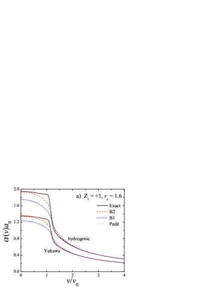
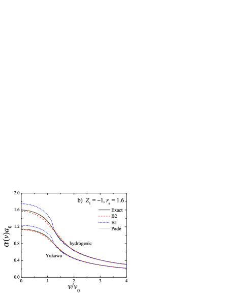
Figure 1: Screening parameter $\alpha(v)a_{0}$ as a function of the ion velocity $v/v_{0}$ for $r_{\mathrm{s}}=1.6$, a) $Z_{1}=+1$, b) $Z_{1}=-1$, calculated with the Yukawa and hydrogenic potentials. The dotted curves corresponding to $\alpha_{\mathrm{B}1}(v)a_{0}$, Eq. (24). The dashed curves indicate the solutions of Eq. (20), i.e. the B2 approximation. The solid curves are the exact screening parameters calculated with Eqs. (9) and (10). Eq. (31) [i.e., the Padé approximant of Eq. (20)] is plotted as thin solid curves.

The exact dynamic screening parameter of $Z_{1}=+1$ (Fig. 1a) displays a conspicuous large negative slope close to the Fermi velocity ($v\simeq v_{\mathrm{F}}\simeq 1.2v_{0}$). In fact the behaviour of $\partial\alpha(v)/\partial v$ is connected, through Eqs. (9) and (10), to the derivative of the dynamic phase shifts, $\partial\Delta_{\ell}(v)/\partial v$. When $v\to v_{\mathrm{F}}$ the latter quantity is finite if $\ell\geqslant 1$ but exhibits a logarithmic singularity if $\ell=0$, $\partial\Delta_{0}(v)/\partial v\sim\lambda_{\mathrm{sc}}\ln|v-v_{\mathrm{F}}|$. Here $\lambda_{\mathrm{sc}}=[\delta_{0}(q)/q]_{q\to 0}$ is the scattering length [7]. The exact theory of low-energy elastic scattering (see, e.g., [7]) predicts a finite scattering length for protons and antiprotons, hence $\partial\alpha(v)/\partial v$ is singular for both types of projectiles. However, $\lambda_{\mathrm{sc}}$ is about two orders of magnitude larger for protons than for antiprotons and the singular behaviour of $\partial\alpha(v)/\partial v$ is clearly visible only for $Z_{1}=+1$. The physical origin of this singularity should be traced to the interaction of the positive ion (with $v=v_{\mathrm{F}}$) with the electrons close to the Fermi surface in which case the relative velocity of the particles can be small. As shown in [5] the cross section of the electron-ion interaction strongly increases for these low-energy (in the relative frame of reference) scattering events with $\ell=0$. This is the so-called resonance scattering investigated first by Wigner and by Bethe and Peierls (see, e.g., [7]).

Finally, we have examined the Padé approximant of order [1/1] to the second-order Born series studied above. Applying this approximant one finds, instead of Eq. (20),

$$\alpha(v)=\alpha_{\mathrm{RPA}}\big{[}\gamma F(s)\big{]}^{1/2}\left[1-\frac{\pi\chi^{2}}{2\gamma}Z_{1}\frac{G(s,u)}{F(s)}\right]^{-1/2}.$$ (31)

The resulting dynamic screening parameters are depicted in Fig. 1. Comparing the different curves displayed in Fig. 1 one concludes that the [1/1] Padé approximant improves the agreement between the B2 approximation and the exact results. The improvement is remarkable for antiprotons where the respective screening parameters agree excellently with the self-consistent treatment based on the dynamic FSR in the whole velocity range.

In conclusion, we have proposed a method to calculate the dynamic screening parameter for an ion moving in a DEG based on the B2 approximation for the FSR. The developed approach furnishes a simple and computationally inexpensive scheme to incorporate the effects of the non-linear ion-solid coupling in the quantum formulation of scattering processes, which is an important prerequisite to describe accurately the non-linear screening and energy loss of ions in solids.

References

- [1] I. Nagy, A. Bergara, Nucl. Instr. Meth. B 115 (1996) 58.
- [2] A.F. Lifschitz, N.R. Arista, Phys. Rev. A 57 (1998) 200.
- [3] E. Zaremba, A. Arnau, P.M. Echenique, Nucl. Instr. Meth. B 96 (1995) 619.
- [4] P.M. Echenique, I. Nagy, A. Arnau, Int. J. Quantum Chem. 23 (1989) 521.
- [5] H.B. Nersisyan, A.K. Das, Nucl. Instr. Meth. B 227 (2005) 455.
- [6] H.B. Nersisyan, J.M. Fernández-Varea, Nucl. Instr. Meth. B 311 (2013) 121.
- [7] L.D. Landau, E.M. Lifshitz, Quantum Mechanics, Gordon and Breach, New York, 1981.
- [8] J. Friedel, Philos. Mag. 43 (1952) 153.
- [9] S. Servadio, Phys. Rev. A 4 (1971) 1256.
- [10] J. Lindhard, K. Dan. Vidensk. Selsk. Mat. Fys. Medd. 28 (1954) 1.
- [11] T.L. Ferrell, R.H. Ritchie, Phys. Rev. B 16 (1977) 115.
- [12] B. Apagyi, I. Nagy, J. Phys. C: Solid State Phys. 20 (1987) 1465.
- [13] A. Ventura, Nuovo Cimento 10D (1988) 43.
- [14] A.H. Sørensen, Nucl. Instr. Meth. B 48 (1990) 10.
- [15] J. Calera-Rubio, A. Gras-Martí, N.R. Arista, Nucl. Instr. Meth. B 93 (1994) 137.
- [16] I. Nagy, B. Apagyi, J.I. Juaristi, P.M. Echenique, Phys. Rev. B 60 (1999) R12546.
- [17] N.R. Arista, A.F. Lifschitz, Nucl. Instr. Meth. B 193 (2002) 8.
- [18] N.R. Arista, A.F. Lifschitz, Adv. Quantum Chem. 45 (2004) 47.
- [19] N.R. Arista, K. Dan. Vidensk. Selsk. Mat. Fys. Medd. 52 (2006) 595.