Coherent backscattering of intense light by cold atoms with degenerate energy levels: Diagrammatic treatment

Abstract

We present a generalization of the diagrammatic pump-probe approach to coherent backscattering (CBS) of intense laser light for atoms with degenerate energy levels. We employ this approach for a characterization of the double scattering signal from optically pumped atoms with the transition $J_{g}\rightarrow J_{e}=J_{g}+1$ in the helicity preserving polarization channel. We show that, in the saturation regime, the internal degeneracy becomes manifest for atoms with $J_{g}\geq 1$, leading to a faster decrease of the CBS enhancement factor with increasing saturation parameter than in the non-degenerate case.

I Introduction

Coherent backscattering (CBS) is an interference phenomenon arising when monochromatic waves get multiply scattered by a disordered distribution of dilute scatterers. It occurs in the weak scattering regime, where the constructive interference of counter-propagating amplitudes survives the disorder average and leads to an enhanced intensity in backscattering direction Lagendijk96 ; sheng . CBS was observed for the first time with optical waves and polystyrene particles acting as classical point scatters albada85 in the 80’s, and, more recently, with acoustic bayer93 , seismic larose04 , and matter josse12 waves.

Constant technical progress and modern cooling techniques made it possible to study CBS of laser light by clouds of cold atoms behaving like unique quantum scatterers labeyrie99 . In contrast to classical scatterers, atoms are able to scatter light inelastically, when driven by an intense resonant laser field cohen-tannoudji . Moreover, the electronic structure of the atoms allows the scattered photons to flip their polarization and renders the scattering process polarization-dependent. Recent experiments on CBS of light by cold Sr chaneliere04 and Rb balik05 atoms showed that nonlinear inelastic scattering, as well as the internal atomic structure strongly affect the phase coherence of the multiply scattered fields, reducing the interference contrast. However, an accurate quantitative description of the above experiments is still missing. Indeed, the theoretical approaches using a diagrammatic scattering theory wellens04 , a master equation shatokhin05 , or quantum Langevin equations gremaud06 led to a deeper understanding of the physical mechanism responsible for the observed coherence loss and achieved a qualitative agreement with the experiment chaneliere04 , but were unable to reach an accurate quantitative description thereof. The major problem with the above approaches is that they are restricted either to a small number of photons or atoms. In particular, the master equation approach is capable of accurately assessing the atomic response to a strong resonant field, but the complexity of the problem increases exponentially with the number of atoms.

Recently, we suggested a hybrid – diagrammatic pump-probe – approach, which blends diagrammatic scattering theory and single-atom master equations (or optical Bloch equations (OBE)) geiger10 ; wellens10 . This method was initially introduced for the double scattering contribution to CBS from two two-level atoms, in which case the signal is deduced from solutions of the OBE under a classical bichromatic driving. One component of the bichromatic driving represents the in general saturating laser field, while the other, non-saturating component stems from the field scattered by the second atom. Thus, our approach owes its name to the analogy with a method in saturation spectroscopy meystre07 .

First of all, since the diagrammatic pump-probe approach uses only single-atom quantities for the derivation of the multiple scattering signal, it circumvents the aforementioned problem of the exponential growth of the system complexity with the number of scatterers. Second, it transforms the problem of CBS of intense laser light off a cold atomic cloud into a form that is amenable to Monte-Carlo simulation methods binninger12 . Third, for double shatokhin10 and triple shatokhin12b scattering orders the solutions obtained within the pump-probe approach are equivalent to the solutions following from the master equation (where, in the triple scattering case, the recurrent scattering contributions are dropped). Under the assumption that this equivalence always holds in the dilute regime, general analytical expressions have recently been derived for single-atom responses shatokhin12b . It will be a subject of future work to include these expressions into the Monte-Carlo simulation subroutines.

The purpose of the present contribution is to generalize the diagrammatic pump-probe approach to realistic dipole transitions possessing internal degeneracy. Such transitions were probed in the above-mentioned experiments chaneliere04 ; balik05 . We will also incorporate a vectorial representation of the electromagnetic fields into our approach, which is required for a proper description of the light-matter interaction as well as of the polarization-sensitive character of the CBS effect.

The paper is structured as follows. In the next section, we recall the basic ingredients of the pump-probe approach for two-level atoms. In Sec. III, we generalize this approach to the scenario of vector fields and atoms with degenerate dipole transitions. Thereafter, we apply this generalized treatment to double scattering from optically pumped atoms with the ground and excited state angular momenta $J_{g}$ and $J_{e}=J_{g}+1$, respectively, in the helicity preserving polarization channel. We show that the elastic component of the double scattering spectrum for arbitrary $J_{g}$ can be expressed using the results for $J_{g}=0$. This is not in general the case for the inelastic intensity, since inelastic scattering from the degenerate ground state results in additional processes that do not interfere perfectly, and lead to a more rapid decay of phase coherence as compared to atoms with $J_{g}=0$. Finally, in Sec. V we conclude our work.

II The diagrammatic pump-probe approach for two-level atoms

Before we present the pump-probe approach to CBS from two atoms with degenerate energy levels, it is instructive to recall its formulation for two-level atoms geiger10 ; wellens10 . The generalization thereof for multilevel dipole transitions will be developed, along the same lines, in Sec. III.

To this end, let us consider double scattering in a toy model of CBS, consisting of two immobile and distant atoms in free space, driven by a near-resonant laser field. The scattering processes which survive the disorder average and contribute to the background and interference intensities, respectively, are shown in Fig. 1(a) and (b). Thick arrows directed towards grey dots depict a cw (continuous wave) laser field of arbitrary strength driving the atoms. Thin solid (dashed) arrows depict positive- (negative-)frequency parts of the scattered field.

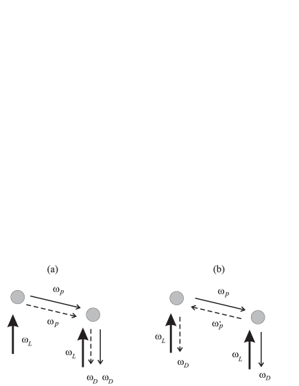
Figure 1: Double scattering processes surviving the disorder average: (a) ladder, or background, contribution, describing co-propagating amplitudes; (b) crossed, or interference, contribution, resulting from the interference between counter-propagating amplitudes. The incident laser field at frequency $\omega_{L}$ is assumed to be strong enough to induce nonlinear inelastic scattering processes, whereupon the frequencies $\omega_{p}$, $\omega_{p}^{\prime}$, and $\omega_{D}$ may differ from the incident laser field’s frequency.

Now, the main idea of the pump-probe approach is to account for the laser-atom interaction non-perturbatively, while the atom-atom interaction is dealt with perturbatively, at lowest non-vanishing order gush74 ; agarwal86 ; mollow72 . The two components of the driving field seen by each of the atoms in Fig. 1 correspond to the incident laser field and the field scattered by the other atom, respectively. A large interatomic separation implies a small Rabi frequency of the scattered field in comparison to the natural line width, and justifies its perturbative treatment. As regards the classical ansatz for the probe field, it was suggested geiger10 ; wellens10 and proven shatokhin10 that it is valid up to second order in the scattered field (two exchanged amplitudes), because the non-classical character of the atomic radiation reveals itself only in the field correlation functions describing the coincidence measurements of at least two photons kimble77 (i.e., four exchanged amplitudes).

The classical description of the scattered fields allows us to consider the light-matter interaction of each of the atoms separately, and to derive the double-scattering signal by combining single-atom building blocks, in analogy with multiple scattering theory Lagendijk96 .

According to geiger10 ; wellens10 , the single-atom building blocks describe stationary spectral responses of a two-level atom subjected to a classical bichromatic electric field $E_{pp}(t)$:

$$E_{pp}(t)=\mathcal{E}e^{-i\omega_{L}t}+\mathcal{E}^{*}e^{i\omega_{L}t}+\epsilon e^{-i\omega_{p}t}+\epsilon^{*}e^{i\omega_{p}t},$$ (1)

where both waves, whose frequencies are introduced in Fig. 1, are split into their positive- and negative-frequency parts, with $\mathcal{E}$ and $\epsilon$ being, respectively, the complex amplitudes of the laser and the scattered fields, the latter acting as a “probe” on the laser-driven atom. Since CBS is observed in the dilute regime, i.e., when $k_{L}r_{12}\gg 1$, the atoms are located in the radiation zone of each other where the probe field scales as $(k_{L}r_{12})^{-1}$, validating a perturbative treatment.

The dynamics of the quantum-mechanical expectation value of an arbitrary atomic observable $Q$ of a two-level atom in free space driven by the classical field (1) can be deduced from a standard master equation for single atom resonance fluorescence under classical bichromatic driving, which in the frame rotating at the laser frequency reads (see, for instance, agarwal86 )

$$\langle\dot{Q}\rangle =\left\langle-i\delta[\sigma^{+}\sigma^{-},Q]-\frac{i}{2}[\Omega\sigma^{+}+\Omega^{*}\sigma^{-},Q]\right.$$

$$\left.+\gamma\left(\sigma^{+}[Q,\sigma^{-}]+[\sigma^{+},Q]\sigma^{-}\right)\right.$$

$$\left.-\frac{i}{2}[ge^{-i\omega t}\sigma^{+}+g^{*}e^{i\omega t}\sigma^{-},Q]\right\rangle.$$ (2)

Here, $\sigma^{-}(\sigma^{+})=\left|g\right>\left<e\right|(\left|e\right>\left<g\right|)$ denotes the atomic lowering (raising) operator, with $\left|g\right>$ and $\left|e\right>$ the atomic ground and excited states, respectively. Furthermore, $\delta=\omega_{L}-\omega_{0}$ is the detuning between the laser and the atomic transition frequency, $\omega=\omega_{p}-\omega_{L}$ the detuning between the probe and the laser field frequency, $\gamma$ half the spontaneous decay rate of the excited state, and $\Omega=2d\mathcal{E}/\hbar$, $g=2d\epsilon/\hbar$, with $d$ the matrix element of the dipole transition, the Rabi frequencies of the laser and probe fields, respectively.

Equation (2) is equivalent to the OBE with bichromatic driving, which we write in matrix form as geiger10 ; wellens10 :

$$\langle\dot{\boldsymbol{\sigma}}(t)\rangle ={\bf M}_{1}\left<\boldsymbol{\sigma}(t)\right>+{\bf L}_{1}+ge^{-i\omega t}\boldsymbol{\Delta}^{(-)}\left<\boldsymbol{\sigma}(t)\right>$$

$$+g^{*}e^{i\omega t}\boldsymbol{\Delta}^{(+)}\left<\boldsymbol{\sigma}(t)\right>.$$ (3)

Here, $\left<\boldsymbol{\sigma}\right>=(\left<\sigma^{-}\right>,\left<\sigma^{+}\right>,\left<\sigma^{z}\right>)$ is the quantum-mechanical expectation value of the optical Bloch vector, with $\sigma^{z}=\sigma^{+}\sigma^{-}-\sigma^{-}\sigma^{+}$, and the explicit form of the matrices $\bf{M}_{1}$, $\boldsymbol{\Delta}^{(+)}$, $\boldsymbol{\Delta}^{(-)}$, together with the vector $\bf{L}_{1}$, is readily obtained when the elements of the Bloch vector are entered into Eq. (2).

The basic quantity that we are using to characterize single-atom stationary spectral responses is the frequency correlation function,

$$I(\nu,\nu^{\prime}) =\frac{1}{(2\pi)^{2}}\int_{-\infty}^{\infty}dt\int_{-\infty}^{\infty}dt^{\prime}e^{-it\nu+it^{\prime}\nu^{\prime}}$$

$$\times\langle\sigma^{+}(t)\sigma^{-}(t^{\prime})\rangle,$$ (4)

which describes spectral correlations between the positive-frequency amplitude at frequency $\nu$ and the negative-frequency amplitude at frequency $\nu^{\prime}$. To evaluate this function, we split the atomic dipole temporal correlation function $\langle\sigma^{+}(t)\sigma^{-}(t^{\prime})\rangle$ in Eq. (4) into a sum of a factorized and a fluctuating part, respectively:

$$\langle\sigma^{+}(t)\sigma^{-}(t^{\prime})\rangle=\langle\sigma^{+}(t)\rangle\langle\sigma^{-}(t^{\prime})\rangle+\langle\Delta\sigma^{+}(t)\Delta\sigma^{-}(t^{\prime})\rangle,$$ (5)

where $\Delta\sigma^{\pm}\equiv\sigma^{\pm}-\langle\sigma^{\pm}\rangle$. Insertion of the right-hand side of Eq. (5) into Eq. (4) yields a decomposition

$$I(\nu,\nu^{\prime})=I^{\rm el}(\nu,\nu^{\prime})+I^{\rm in}(\nu,\nu^{\prime}),$$ (6)

where elastic and inelastic components, $I^{\rm el}(\nu,\nu^{\prime})$ and $I^{\rm in}(\nu,\nu^{\prime})$, result from the Fourier transform of the factorized and the fluctuating part of the atomic dipole correlation function (5), respectively.

The stationary factorized atomic dipole correlation function, defined in terms of the atomic raising and lowering operators, can readily be evaluated from the perturbative solutions of Eq. (II) to second order in the probe field amplitude. A similar consideration applies also to the fluctuating part of the atomic dipole correlation function, since, according to the quantum regression theorem cohen-tannoudji , it satisfies an equation of motion which follows straightforwardly from (II). Plugging the obtained solutions into Eq. (4), and performing the Fourier transformations, we obtain the elastic and inelastic single atom-spectral responses.

In frequency space, the perturbative solutions for the atomic dipole averages and correlation functions are referred to as the elementary single-atoms building blocks.

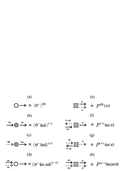
Figure 2: Graphical definitions of the elementary single-atom spectral responses, together with our notation for the corresponding correlation functions. (a)-(d) complex scattering amplitudes associated with the perturbative solutions of Eq. (II); (e)-(h) blocks associated with the perturbative solutions for the fluctuating part of the atomic dipole correlation function $\langle\Delta\sigma^{+}(t)\Delta\sigma^{-}(t^{\prime})\rangle$ (see Eq. (5)). Blank and hatched shapes denote elastic and inelastic spectral responses, respectively (see text).

It is convenient to define them graphically shatokhin12a . Figure 2 shows the complete set of the elementary blocks, together with their symbolic expressions, that are required for the construction of the double scattering ladder and crossed spectra. As seen from Fig. 2, the frequencies of incoming and outgoing amplitudes are correlated, which is a direct consequence of energy conservation during the scattering processes wellens10 ; geiger10 .

Furthermore, it should be mentioned that, for each of the elementary blocks, a replacement of solid arrows with dashed ones and vice versa yields complex conjugated blocks. Therefore, knowledge of the spectral responses shown in Fig. 2 suffices to obtain an arbitrary single-atom spectral response needed to infer the double scattering signal. Circles with one outgoing solid arrow [see Figs. 2(a)-(d)] provide graphical representations of the perturbative corrections of zeroth (no incoming arrows), first (one incoming solid or dashed arrow), and second order (one dashed and one solid incoming arrows) to the expectation value of the atomic dipole lowering operator $\langle\sigma^{-}\rangle$. Squares with two outgoing arrows [see Figs. 2(e)-(h)] correspond to the perturbative solutions for the inelastic component of the frequency correlation function (4). We put labels above the arrows to denote the detunings of the corresponding waves from the laser field frequency; in case of exact resonance, the labels are omitted for brevity. Furthermore, we leave a shape blank if its outgoing arrow is elastic with respect to the laser frequency (in case of the squares, this rule applies to the arrow that is directed towards the detector if the detected field is elastic with respect to the laser frequency, see e.g. Fig. 3). Otherwise, the shape is hatched. The expressions for the correlation functions on the right hand sides of each of the diagrams in Fig. 2 can be found in shatokhin12a .

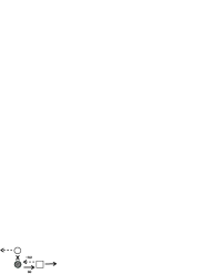
Figure 3: An example of a double scattering diagram contributing to the elastic crossed spectrum. The spectral response of the left atom is elastic, and constructed as a product (denoted by the ‘X’) of the block which is the complex conjugate of the one shown in Fig. 2(a), and of the block Fig. 2(c) (one should bear in mind that, for circles, the direction of the outgoing arrow is immaterial for the definition of the spectral response shatokhin12a ). The spectral response of the right atom is represented by the block in Fig. 2(f). There is no hatching of the square since, as discussed in the text, the outgoing arrow that represents the detected field is elastic with respect to the laser frequency. The overall mathematical expression for this double scattering process is given in Eq. (7).

To construct double scattering processes contributing to the ladder or crossed signals, one decomposes the total spectral response of each of the two atoms into its elastic and inelastic components, using the elementary building blocks from Fig. 2 and their complex conjugates shatokhin12a . Then the diagrammatic expansions for both atoms are reconnected self-consistently, using a set of rules shatokhin12a , to form double scattering diagrams of either ladder [see Fig. 1(a)] or crossed [see Fig. 1(b)] types. We present an example of a double scattering diagram contributing to the elastic crossed spectrum in Fig. 3. Applying the rules of self-consistent combination of the building blocks to the relevant spectral response functions (see Fig. 2), we obtain

$${\rm Fig}.~{}\ref{fig:examp_cross}=|\bar{g}|^{2}\int_{-\infty}^{\infty}\frac{d\omega}{2\pi}\langle\sigma^{+}\rangle^{(0)}\langle\sigma^{-}(-\omega)\rangle^{(+)}P^{(-)}(\omega,0),$$ (7)

where $\bar{g}\propto(k_{L}\ell)^{-1}$, with $\ell$ the average interatomic distance. Detailed expressions and numerous examples of the double scattering elastic and inelastic spectra can be found in geiger09 .

Concluding this section, we would like to mention that the elementary single-atom blocks have a physical interpretation as effective nonlinear susceptibilities shatokhin12a , which describe the response of the laser-driven atom to weak probe fields boyd . Recently, it has been shown that there is a systematic way of obtaining analytical expressions for such blocks in case of an arbitrary number of probe fields shatokhin12b . In future work, these expressions will be incorporated into the theory of nonlinear transport by classical scatterers wellens08 to describe CBS of intense laser light in cold atomic gases binninger12 .

III Generalization of the approach to atoms with degenerate dipole transitions

III.1 Fundamental double scattering processes

The diagrammatic pump-probe approach, presented in the previous section, ignores the polarization degree of freedom of the light. This is closely related to the fact that, in Sec. II, we reduced the internal quantum structure of the atomic dipole transitions to one ground and one excited level. However, Sr or Rb atoms, studied in real experiments on CBS of light, possess degenerate dipole transitions, what renders this effect sensitive to the choice of the incoming and outgoing fields’ polarizations labeyrie03 ; kupriyanov06 . Our main goal will be to include the internal degeneracy, as well as the vector character of the electromagnetic field, into the diagrammatic pump-probe approach. As in the case of scalar atoms, we will ensure, whenever possible, a close correspondence with the results of the master equation approach. Presently, such results have been made available for double scattering from two Sr atoms shatokhin05 ; shatokhin07 ; ralf11 .

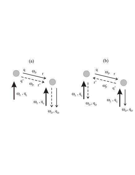
Figure 4: Double scattering diagrams which survive the disorder average – for the case of vector electric fields, and atoms with degenerate dipole transitions: (a) ladder spectrum; (b) crossed spectrum. The meaning of the labels $\omega_{L}$, $\omega_{p}$, $\omega_{p}^{\prime}$, and $\omega_{D}$ is the same as in Fig. 1. Indices $q_{L}$, $q$, $q^{\prime}$, $r$, $r^{\prime}$, and $q_{D}$ refer to the polarization indices of the corresponding arrows in the spherical basis (see text for further details).

Inclusion of polarization and electronic degeneracy amounts to a certain technical overhead, without affecting the basic idea of the approach. Namely, the matrix dimension of the linear system generalizing Eq. (II) will increase according to the number of sublevels of the electronic ground and excited states. Furthermore, the explicit form of the single-atom building blocks will now depend on the choices of the pump, probe, and detected fields’ polarizations. However, our justification of the classical description of the exchanged amplitudes, as presented in Sec. II, certainly remains true also for polarized electric fields.

To begin with, let us consider a vectorial generalization of the fundamental scattering processes (see Fig. 1) that survive the disorder average in Fig. 4. Co-propagating inelastic scattering amplitudes contribute to the ladder spectrum [see Fig. 4(a)], and counter-propagating amplitudes contribute to the crossed spectrum [see Fig. 4(b)]. In addition to the elements that are present in Fig. 1, each of the arrows in Fig. 4 is now garnished by polarization indices. Unless otherwise stated, any such index $q$ corresponds to a unit polarization vector $\hat{\bf e}_{q}$ in the spherical basis:

$$\hat{\bf e}_{\pm 1}=\mp\frac{1}{\sqrt{2}}\left(\hat{\bf e}_{x}\pm i\hat{\bf e}_{y}\right),\quad\hat{\bf e}_{0}=\hat{\bf e}_{z},$$ (8)

where $\hat{\bf e}_{x}$, $\hat{\bf e}_{y}$, and $\hat{\bf e}_{z}$ are the unit vectors in the Cartesian basis.

In general, arrows corresponding to the scattered fields carry a pair of polarization indices. However, we will study the CBS signal in exact backscattering direction, that is, along the quantization axis set by the direction of the laser wave. Therefore, the polarization of the backscattered field, alike the laser field, can be specified by a single index.

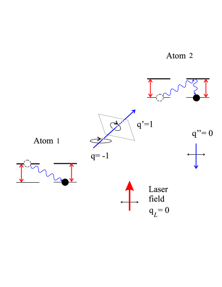
Figure 5: (Color online) A linearly polarized laser wave (thick red arrow) excites the $\pi$-transitions (double red thin arrows) of two atoms with ground and excited state angular momenta $J_{g}$ and $J_{e}$ equal to $1/2$. Atom 1 emits a $\sigma_{-}$ polarized amplitude ($q=-1$) towards atom 2, and, after projection of the polarization vector onto the plane perpendicular to the line connecting both atoms, excites a $\sigma_{+}$-transition thereof ($q^{\prime}=+1$). Finally, a $\pi$-polarized amplitude ($q^{\prime\prime}=0$) is emitted by atom 2 towards the detector.

Introducing a pair of polarization indices for the intermediate arrows can be motivated with the aid of Fig. 5, which presents an example of a double scattering process of a linearly polarized positive-frequency laser wave by two atoms with equal angular momenta of the ground and excited states: $J_{g}=J_{e}=1/2$. As evident from Fig. 5, the polarizations of the waves emitted by atom 1 ($q=-1$) and absorbed by atom 2 ($q^{\prime}=+1$) can be different, hence the two indices for the intermediate amplitudes. For the positive-frequency wave, the probability amplitudes of various combinations of $q,q^{\prime}$ are defined by the projections thereof on the plane transverse to the line connecting the atoms (see Fig. 5), given by $\overleftrightarrow{\boldsymbol{\Delta}}_{q^{\prime}q}\equiv\hat{\bf e}^{*}_{q^{\prime}}\cdot\overleftrightarrow{\boldsymbol{\Delta}}\cdot\hat{\bf e}_{q}$, with the projector on the transverse plane $\overleftrightarrow{\boldsymbol{\Delta}}=\overleftrightarrow{\openone}-\hat{\bf n}\hat{\bf n}$, and

$$\overleftrightarrow{\openone} =-\hat{\bf e}_{-1}\hat{\bf e}_{+1}+\hat{\bf e}_{0}\hat{\bf e}_{0}-\hat{\bf e}_{+1}\hat{\bf e}_{-1},$$ (9)

$$\hat{\bf n} =\frac{e^{i\phi}\sin\vartheta}{\sqrt{2}}\hat{\bf e}_{-1}+\cos\vartheta\hat{\bf e}_{0}-\frac{e^{-i\phi}\sin\vartheta}{\sqrt{2}}\hat{\bf e}_{+1}.$$ (10)

By analogy, it is easy to show that the complex conjugate amplitude of the one shown in Fig. 5 is proportional to $(\overleftrightarrow{\boldsymbol{\Delta}}_{q^{\prime}q})^{*}=\hat{\bf e}^{*}_{q}\cdot\overleftrightarrow{\boldsymbol{\Delta}}\cdot\hat{\bf e}_{q^{\prime}}$.

It follows from the above that the double scattering processes shown in Figs. 4(a) and 4(b) are proportional to the geometric factor $({\bf e}_{r}^{*}\cdot\overleftrightarrow{\boldsymbol{\Delta}}\cdot\hat{\bf e}_{q})({\bf e}^{*}_{q^{\prime}}\cdot\overleftrightarrow{\boldsymbol{\Delta}}\cdot\hat{\bf e}_{r^{\prime}})$, whose explicit form can easily be obtained for arbitrary polarization indices using Eqs. (9), (10). Next, we need to perform the configuration average over the random angles $(\vartheta,\phi)$ – which define the orientation of the vector $\hat{\bf n}$ connecting the atoms with respect to the quantization axis [see Eq. (10)]. The resulting geometric weight for diagrams in Fig. 4(a),(b) reads

$$\langle\overleftrightarrow{\boldsymbol{\Delta}}_{rq}\overleftrightarrow{\boldsymbol{\Delta}}_{q^{\prime}r^{\prime}}\rangle=\frac{1}{4\pi}\int_{0}^{\pi}\sin\vartheta d\vartheta\int_{0}^{2\pi}\overleftrightarrow{\boldsymbol{\Delta}}_{rq}\overleftrightarrow{\boldsymbol{\Delta}}_{q^{\prime}r^{\prime}}d\phi.$$ (11)

Finally, if there are several polarization channels for double scattering, we perform a summation over the corresponding polarization indices.

Each of the disorder-averaged geometric weights must be multiplied by the corresponding double scattering spectral response, whose evaluation from single-atom building blocks will be considered in the subsequent sections.

III.2 Diagrammatic expansion of the double scattering process

After selecting the double scattering processes which survive the disorder average, we proceed by considering the two atoms and their incoming and outgoing classical fields in Fig. 4(a),(b) separately. In complete analogy with the case of scalar atoms geiger10 ; wellens10 ; shatokhin12a , the spectral response of either one of the atoms is split into an elastic and an inelastic component. It is convenient to represent these components graphically, as shown in Figs. 6 and 7.

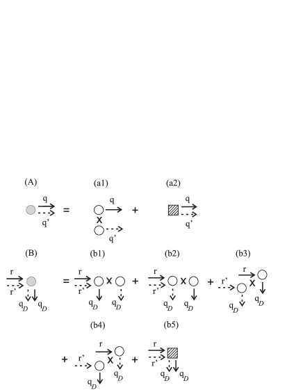
Figure 6: Diagrammatic expansion of the double scattering process depicted in Fig. 4(a) into its elastic (blank circles) and inelastic (hatched boxes) components. Left (A, B): Single-atom building blocks contributing to the ladder spectrum. Right (a1-b5): Expansion of the single-atom building blocks into elementary building blocks.

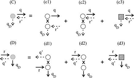
Figure 7: Diagrammatic expansion of the double scattering process depicted in Fig. 4(b) into the elastic (blank circles) and inelastic (hatched boxes) components. Left (C, D): Single-atom building blocks contributing to the crossed spectrum. Right (c1-d3): Expansion of the single-atom building blocks into elementary building blocks.

We remind that, to alleviate the diagrams, the arrows which represent the laser field are not depicted in Figs. 6 and 7. Note also that we do not yet assign the frequency values to different arrows in Figs. 6, 7: these will be determined in the course of a self-consistent combination of the single-atom responses into double scattering ladder and crossed spectral signals (see Sec. III.6). To facilitate establishing the correspondence between the diagrams in Figs. 6, 7 and 4, respectively, we depict the backscattered fields with downward-directed arrows.

In each of these graphical equations, open circles with one outgoing arrow and null, one or two incoming arrows describe the elementary elastic building blocks. Circles are always combined in pairs by the symbols X. We will see below, in Sec. III.5.1, that pairs of circles correspond to the factorized parts of the atomic dipole correlation function, which describe the elastic spectral responses. The number of pairs of circles in the graphical expansion of the building blocks is equal to $2^{n}$, where $n$ is the number of incoming probe fields shatokhin12a ; shatokhin12b .

Apart from the open circles, each of the graphical equations in Figs. 6, 7 contains one hatched square, with two outgoing arrows and null, one or two incoming arrows. This corresponds to the inelastic elementary building block, which can be derived from the fluctuating part of the atomic dipole correlation function, see Sec. III.5.2.

Computation of the single-atom elementary elastic and inelastic spectral responses is based on the formalism of the generalized OBE, to be explained below.

III.3 Generalized optical Bloch equations

This section presents a step-by-step generalization of the OBE formalism outlined in Sec. II, to the case of vector fields and atoms with arbitrary dipole transitions. We set out by writing down the expression for the classical bichromatic vector field

$${\bf E}_{pp}(t)=\mathcal{E}\hat{\bf e}_{L}e^{-i\omega_{L}t}+\mathcal{E}^{*}\hat{\bf e}^{*}_{L}e^{i\omega_{L}t}+\epsilon\hat{\bf e}_{r}e^{-i\omega_{p}t}+\epsilon^{*}\hat{\bf e}^{*}_{r^{\prime}}e^{i\omega_{p}t},$$ (12)

where the meaning of $\mathcal{E}$, $\epsilon$, $\omega_{L}$, $\omega_{p}$ is the same as in Eq. (1), and $\hat{\bf e}_{L}$, $\hat{\bf e}_{r}$ ($\hat{\bf e}^{*}_{r^{\prime}}$) are the unit polarization vectors of the laser and probe fields, respectively.

To account for the vector nature of the atomic dipole transition, we introduce vector raising and lowering atomic operators instead of the operators $\sigma^{+}$ and $\sigma^{-}$. We will consider atoms with total ground and excited state angular momenta $J_{g}$ and $J_{e}$, respectively. Then the atomic raising and lowering operators, ${\bf D}^{\dagger}$ and ${\bf D}$, can be expressed using the projection operators on the ground and excited state manifolds:

$$P_{e}=\sum_{m_{e}=-J_{e}}^{J_{e}}|J_{e}m_{e}\rangle\langle J_{e}m_{e}|,\;P_{g}=\sum_{m_{g}=-J_{g}}^{J_{g}}|J_{g}m_{g}\rangle\langle J_{g}m_{g}|,$$ (13)

where $|J_{e}m_{e}\rangle$ ($|J_{g}m_{g}\rangle$) denotes an excited (ground) state sublevel with magnetic quantum number $m_{e}$ ($m_{g}$). The raising and lowering parts of the atomic dipole operator read

$${\bf D}^{\dagger}=\frac{1}{d}P_{e}\boldsymbol{\cal D}P_{g},\quad{\bf D}=({\bf D}^{\dagger})^{\dagger},$$ (14)

where $d\equiv\langle J_{e}||{\cal D}||J_{g}\rangle$ is the reduced matrix element, and $\boldsymbol{\cal D}=d({\bf D}^{\dagger}+{\bf D})$ is the atomic dipole moment operator. Inserting the projectors (13) into Eq. (14), and using the Wigner-Eckart theorem sakurai , we obtain the following expression

$${\bf D}^{\dagger}=\!\!\sum_{q=-1}^{1}\sum_{m_{g}=-J_{g}}^{J_{g}}\!\!\!\hat{\bf e}_{q}^{*}\langle J_{g}m_{g},1q|J_{e}m_{g}+q\rangle|J_{e}m_{g}+q\rangle\langle J_{g}m_{g}|,$$ (15)

where $\langle J_{g}m_{g},1q|J_{e}m_{g}+q\rangle$ denotes a Clebsch-Gordan coefficient, and one summation (over $m_{e}$) was removed from Eq. (15) owing to the dipole transition selection rules sakurai .

With the vector bichromatic field and dipole operators defined, we merely make the replacements $E_{pp}(t)\rightarrow{\bf E}_{pp}(t)$, $\sigma^{+}\rightarrow{\bf D}^{\dagger}$, $\sigma^{-}\rightarrow{\bf D}$ in Eq. (2), to obtain its vector generalization:

$$\langle\dot{Q}\rangle =\left\langle\!-i\delta[{\bf D}^{\dagger}\!\cdot\!{\bf D},Q]\!-\!\frac{i}{2}[\Omega({\bf D}^{\dagger}\!\cdot\!\hat{\bf e}_{L})\!+\!\Omega^{*}({\bf D}\!\cdot\!\hat{\bf e}_{L}^{*}),Q]\right.$$

$$\left.+\gamma\left({\bf D}^{\dagger}\cdot[Q,{\bf D}]+[{\bf D}^{\dagger},Q]\cdot{\bf D}\right)\right.$$

$$\left.-\frac{i}{2}[ge^{-i\omega t}({\bf D}^{\dagger}\cdot\hat{\bf e}_{r})+g^{*}e^{i\omega t}({\bf D}\cdot\hat{\bf e}_{r^{\prime}}^{*}),Q]\right\rangle.$$ (16)

Finally, by choosing operators $Q$ from the complete set of operators (see Appendix A), we translate the master equation (16) into a matrix equation for the vector $\langle{\bf Q}\rangle$, in full analogy with the case of a two-level atom [see Eq. (II)]. Accordingly, we will refer to the resulting system of equations,

$$\langle\dot{\bf Q}\rangle ={\bf M}\langle{\bf Q}\rangle+{\bf L}+ge^{-i\omega t}\boldsymbol{\Delta}_{r}^{(-)}\langle{\bf Q}\rangle$$

$$+g^{*}e^{i\omega t}\boldsymbol{\Delta}_{r^{\prime}}^{(+)}\langle{\bf Q}\rangle,$$ (17)

as the generalized optical Bloch equations under bichromatic driving.

III.4 Single-atom spectral correlation functions

We characterize the spectral response of multilevel atoms in different polarization channels by the tensor frequency correlation function generalizing Eq. (4):

$$I_{q^{\prime}q}(\nu^{\prime},\nu) =\frac{1}{(2\pi)^{2}}\int_{-\infty}^{\infty}dt\int_{-\infty}^{\infty}dt^{\prime}e^{-it^{\prime}\nu^{\prime}+it\nu}$$

$$\times\langle D^{\dagger}_{q^{\prime}}(t^{\prime})D_{q}(t)\rangle,$$ (18)

where $D^{\dagger}_{q^{\prime}}(t^{\prime})\equiv\hat{\bf e}_{q^{\prime}}\cdot{\bf D}^{\dagger}(t^{\prime})$ and $D_{q}(t)\equiv\hat{\bf e}^{*}_{q}\cdot{\bf D}(t)$. In complete analogy with the scalar case, we proceed by decomposing the atomic dipole correlation function in (18) into a factorized and a fluctuating part:

$$\langle D^{\dagger}_{q^{\prime}}(t^{\prime})D_{q}(t)\rangle=\langle D^{\dagger}_{q^{\prime}}(t^{\prime})\rangle\langle D_{q}(t)\rangle+\langle\Delta D^{\dagger}_{q^{\prime}}(t^{\prime})\Delta D_{q}(t)\rangle,$$ (19)

with the fluctuating part $\Delta D_{q}$ defined in strict analogy to Eq. (5). Both of the correlation functions on the right hand side of Eq. (19) can be found by solving Eq. (17). Plugging the right hand side of Eq. (19) into Eq. (18), we obtain a tensor correlation function which generalizes Eq. (6):

$$I_{q^{\prime}q}(\nu^{\prime},\nu)=I^{\rm el}_{q^{\prime}q}(\nu^{\prime},\nu)+I^{\rm in}_{q^{\prime}q}(\nu^{\prime},\nu).$$ (20)

Once again, the elastic and inelastic components arise from the factorized and fluctuating parts of the atomic dipole correlation function, respectively. Apart from the frequencies $\nu$, $\nu^{\prime}$ and polarization indices $q,q^{\prime}$, the correlation functions in Eq. (20) depend also on the frequency $\omega$ and the polarization indices $r$, $r^{\prime}$ of the incoming wave. These dependencies will be reflected in the diagrammatic representation of the single atom blocks, to be introduced below.

III.5 Building blocks

The evaluation of the single-atom building blocks in the vectorial case is again completely analogous to the scalar one. To see this, it is important to realize that, regardless of the structure of the dipole transition and the polarization indices of the driving and scattered fields, the spectral response functions, expanded to second order in the probe field amplitude, satisfy the same energy conservation conditions as their scalar analogs studied in detail in wellens10 ; geiger10 . Namely, the response functions contain $\delta$-functions originating from integrations over time in Eq. (18), under the assumption of stationarity of the atomic dipole correlation functions $\langle D^{\dagger}_{q^{\prime}}(t^{\prime})D_{q}(t)\rangle=\langle D^{\dagger}_{q^{\prime}}(t^{\prime}-t)D_{q}(0)\rangle$, what entails strict relations between the incoming and outgoing frequencies.

We incorporate these relations into the diagrammatic representation of the elementary single-atom building blocks (see Fig. 8).

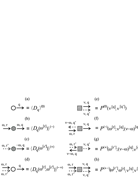
Figure 8: Elementary single-atom building blocks, together with the corresponding spectral response functions in the vector case. (a)-(d) Complex scattering amplitudes associated with the perturbative solutions of Eq. (17); (e)-(h) blocks associated with the perturbative solutions for the fluctuating part of the atomic dipole correlation function, see Eq. (19). The notation $\omega^{[q]}$ for a positive-(negative-)frequency wave implies a wave with frequency $\omega$ and polarization described by the unit vector $\hat{\bf e}_{q}$ ($\hat{\bf e}_{q}^{*}$). Blank and hatched shapes denote elastic and inelastic spectral responses, respectively, in full analogy to the scalar case, see Fig. 2.

As seen from Fig. 8, we introduce the same type (elastic or inelastic) and number of the spectral response functions as in the scalar case (see Fig. 2). In addition to the graphical elements that are already present in the scalar case, each incoming and outgoing arrow in Fig. 8 carries a polarization index.

We will now explain how to find explicit expressions for the vector spectral responses on the right hand sides of the graphical equations in Fig. 8.

III.5.1 Elastic building blocks

All the elastic spectral response functions appearing on the right hand side in Fig. 8(a)-(d) can be obtained directly from the stationary perturbative solutions of the generalized OBE (17), to second order in the probe field amplitude. Setting the left hand side of Eq. (17) to zero, it is easy to obtain the following perturbative solutions:

$$\langle{\bf Q}\rangle^{(0)} ={\bf G}{\bf L},$$ (21a)

$$\langle{\bf Q}(\omega^{[r]})\rangle^{(-)} ={\bf G}(-i\omega)\boldsymbol{\Delta}^{(-)}_{r}\langle{\bf Q}\rangle^{(0)},$$ (21b)

$$\langle{\bf Q}(\omega^{[r^{\prime}]})\rangle^{(+)} ={\bf G}(i\omega)\boldsymbol{\Delta}^{(+)}_{r^{\prime}}\langle{\bf Q}\rangle^{(0)},$$ (21c)

$$\langle{\bf Q}(\omega^{[r]},\omega^{[r^{\prime}]})\rangle^{(-+)} ={\bf G}\boldsymbol{\Delta}^{(+)}_{r^{\prime}}\langle{\bf Q}(\omega^{[r]})\rangle^{(-)}$$

$$+{\bf G}\boldsymbol{\Delta}^{(-)}_{r}\langle{\bf Q}(\omega^{[r^{\prime}]})\rangle^{(+)},$$ (21d)

where

$${\bf G}(z)=\frac{1}{z-{\bf M}}$$ (22)

is the free propagator governing the internal dynamics of the laser-driven, damped atom, and ${\bf G}\equiv{\bf G}(0)$.

Using the perturbative solutions (21), the expressions for the elementary blocks with one solid (dashed) outgoing arrow carrying the index $q$ [see Figs. 8(a)-(d)] can be expressed as scalar products with the projection vectors ${\bf V}_{q}$ (${\bf U}_{q}$), respectively (see Appendix A). For example, the zeroth-order projections yield

$$\langle D_{q}\rangle^{(0)}={\bf V}_{q}\cdot\langle{\bf Q}\rangle^{(0)},\quad\langle D^{\dagger}_{q}\rangle^{(0)}={\bf U}_{q}\cdot\langle{\bf Q}\rangle^{(0)}.$$ (23)

The remaining elementary building blocks are constructed analogously.

III.5.2 Inelastic building blocks

The starting point for the derivation of the inelastic building blocks is the introduction of the stationary vector correlation functions

$${\bf f}_{q}(\tau) =\langle\Delta{\bf Q}(\tau)\Delta D_{q}\rangle,$$ (24a)

$${\bf h}_{q^{\prime}}(\tau) =\langle\Delta D^{\dagger}_{q^{\prime}}\Delta{\bf Q}(\tau)\rangle,$$ (24b)

where $\tau\geq 0$.

Application of the quantum regression theorem to Eq. (24a) leads to the following equation of motion for the vector ${\bf f}_{q}$ [compare with Eq. (17)]:

$$\dot{\bf f}_{q}={\bf Mf}_{q}+ge^{-i\omega t}\boldsymbol{\Delta}_{r}^{(-)}{\bf f}_{q}+g^{*}e^{i\omega t}\boldsymbol{\Delta}_{r^{\prime}}^{(+)}{\bf f}_{q},$$ (25)

and the equation for ${\bf h}_{q^{\prime}}$ is obtained upon replacing ${\bf f}_{q}\rightarrow{\bf h}_{q^{\prime}}$. The temporal evolutions of the vector functions ${\bf f}_{q}$ and ${\bf h}_{q^{\prime}}$ are, of course, different from each other, due to the different initial conditions, ${\bf f}_{q}(0)\neq{\bf h}_{q^{\prime}}(0)$, see Eq. (24). We solve Eq. (25) perturbatively using Laplace transform; the solutions for ${\bf h}_{q^{\prime}}$ follow by analogy. As we will see below, Laplace transforms of ${\bf f}_{q}$ and ${\bf h}_{q^{\prime}}$ define the outgoing negative-frequency amplitude with polarization $q^{\prime}$ and positive-frequency amplitude with polarization $q$, respectively, of the inelastic building blocks in Figs. 8(e)-(h). We have

$$\tilde{\bf f}^{(0)}_{q}(z^{\prime\prime}) ={\bf G}(iz^{\prime\prime}){\bf f}^{(0)}_{q}(0),$$ (26a)

$$\tilde{\bf f}^{(+)}_{q}(\omega^{[r^{\prime}]};z^{\prime\prime}) ={\bf G}(iz^{\prime\prime}+i\omega)\left\{\boldsymbol{\Delta}^{(+)}_{r^{\prime}}\tilde{\bf f}^{(0)}_{q}(z^{\prime\prime})+{\bf f}^{(+)}_{q}(\omega^{[r^{\prime}]};0)\right\},$$ (26b)

$$\tilde{\bf f}^{(-)}_{q}(\omega^{[r]};z^{\prime\prime}) ={\bf G}(iz^{\prime\prime}-i\omega)\left\{\boldsymbol{\Delta}^{(-)}_{r}\tilde{\bf f}^{(0)}_{q}(z^{\prime\prime})+{\bf f}^{(-)}_{q}(\omega^{[r]};0)\right\},$$ (26c)

$$\tilde{\bf f}^{(+-)}_{q}(\omega^{[r^{\prime}]},\omega^{[r]};z^{\prime\prime}) ={\bf G}(iz^{\prime\prime})\left\{\boldsymbol{\Delta}^{(-)}_{r}\tilde{\bf f}^{(+)}_{q}(\omega^{[r^{\prime}]};z^{\prime\prime})+\boldsymbol{\Delta}^{(+)}_{r^{\prime}}\tilde{\bf f}^{(-)}_{q}(\omega^{[r]};z^{\prime\prime})+{\bf f}^{(+-)}_{q}(\omega^{[r^{\prime}]},\omega^{[r]};0)\right\},$$ (26d)

where $z^{\prime\prime}={\rm Im}(z)$, and the vectors of the initial conditions ${\bf f}^{(0)}_{q}(0)$, ${\bf f}^{(+)}_{q}(\omega^{[r^{\prime}]};0)$, ${\bf f}^{(-)}_{q}(\omega^{[r]};0)$ and ${\bf f}^{(+-)}_{q}(\omega^{[r^{\prime}]},\omega^{[r]};0)$ are given in Appendix B. Now, the outgoing positive- and negative-frequency fields of the inelastic building blocks follow via scalar products of the obtained perturbative solutions with the projection vectors ${\bf V}_{q}$ and ${\bf U}_{q^{\prime}}$, respectively, yielding the following expressions for the inelastic building blocks:

$$P^{(0)}(\nu^{[q]},\nu^{[q^{\prime}]}) ={\bf U}_{q^{\prime}}\cdot\tilde{\bf f}^{(0)}_{q}(\nu)+{\bf V}_{q}\cdot\tilde{\bf h}^{(0)}_{q^{\prime}}(-\nu),$$ (27a)

$$P^{(-)}(\omega^{[r]};\nu^{[q]},(\nu-\omega)^{[q^{\prime}]}) ={\bf U}_{q^{\prime}}\cdot\tilde{\bf f}^{(-)}_{q}(\omega^{[r]};\nu)+{\bf V}_{q}\cdot\tilde{\bf h}^{(-)}_{q^{\prime}}(\omega^{[r]};\omega-\nu),$$ (27b)

$$P^{(+)}(\omega^{[r^{\prime}]};(\nu-\omega)^{[q]},\nu^{[q^{\prime}]}) ={\bf U}_{q^{\prime}}\cdot\tilde{\bf f}^{(+)}_{q}(\omega^{[r^{\prime}]};\nu-\omega)+{\bf V}_{q}\cdot\tilde{\bf h}^{(+)}_{q^{\prime}}(\omega^{[r^{\prime}]};-\nu),$$ (27c)

$$P^{(+-)}(\omega^{[r^{\prime}]},\omega^{[r]};\nu^{[q]},\nu^{[q^{\prime}]}) ={\bf U}_{q^{\prime}}\cdot\tilde{\bf f}^{(+-)}_{q}(\omega^{[r^{\prime}]},\omega^{[r]};\nu)+{\bf V}_{q}\cdot\tilde{\bf h}^{(+-)}_{q^{\prime}}(\omega^{[r^{\prime}]},\omega^{[r]};-\nu),$$ (27d)

with the values of $z$ in every expression above fixed by the energy conservation relation, in strict analogy with the scalar case geiger10 .

III.6 Self-consistent combination of single-atom building blocks

In the previous section we defined the elementary single-atom building blocks. Now, we will discuss the rules of their self-consistent combination into double-scattering contributions to CBS. For non-degenerate dipole transitions, these rules were elaborated in shatokhin12a ; shatokhin12b .

As already mentioned in Sec. III.5, for fixed values of the polarization indices, the number of the elementary elastic and inelastic response functions is the same as in the scalar case. Furthermore, these response functions exhibit the same relations between the frequencies of the incoming and outgoing fields. Therefore, the rules of the self-consistent combination that were formulated for non-degenerate dipole transitions are valid also in the present case.

To be self-contained, we here briefly remind the reader of how to construct the double scattering signal using single-atom responses. To obtain the ladder spectrum, we connect the outgoing arrows of each of the diagrams on the right hand side of the graphical equation (A) with the incoming arrows of those of equation (B) in Fig. 6, respecting the direction and character (solid or dashed) of the arrows. The frequency values of all the arrows are assigned according to the definitions of the elementary single-atom building blocks given in Fig. 8. If the frequency of an intermediate arrow that is distinct from the laser frequency changes its value upon the scattering process, it is integrated over. Finally, the two downward arrows corresponding to the backscattered signal in a given polarization channel should bear the same polarization indices and frequency values (equal to $\nu$ for the inelastic component). Application of these rules to the diagrammatic expansions (A) and (B) in Fig. 6 results in six contributions – (a1)(b1), (a1)(b2), (a1)(b3), (a1)(b4), (a2)(b1), (a2)(b2) – to the elastic, and four contributions – (a1)(b5), (a2)(b3), (a2)(b4), (a2)(b5) – to the inelastic component of the double scattering ladder spectrum. For example, the combination of diagrams (a2) and (b5) in Fig. 6 yields the result

$${\rm(a2)(b5)} =|\bar{g}|^{2}\langle\overleftrightarrow{\boldsymbol{\Delta}}_{qr}\overleftrightarrow{\boldsymbol{\Delta}}_{r^{\prime}q^{\prime}}\rangle\int_{\infty}^{\infty}\frac{d\omega}{2\pi}P^{(0)}(\omega^{[q]},\omega^{[q^{\prime}]})$$

$$\times P^{(+-)}(\omega^{[r^{\prime}]},\omega^{[r]};\nu^{[q_{D}]},\nu^{[q_{D}]}).$$ (28)

Using this example, it is easy to construct the expressions for other contributions by analogy.

To obtain the crossed signal, we apply the same rules to the graphical equations (C) and (D) in Fig. 7. Here, a subtlety arises when combining diagrams (c2) and (d2). Such a combination is forbidden since it features a closed loop including two amplitudes cycling between the two circles without an outgoing amplitude wellens08 ; shatokhin12a ; shatokhin12b . Excluding the forbidden diagram, we obtain five contributions – (c1)(d1), (c1)(d2), (c2)(d1), (c2)(d3), and (c3)(d2) to the elastic, and three contributions – (c1)(d3), (c3)(d1), and (c3)(d3) – to the inelastic spectrum of CBS.

Finally, after summation over the relevant values of the intermediate polarization indices $q$, $q^{\prime}$, $r$, and $r^{\prime}$, one obtains the result for the double scattering ladder and crossed spectra in a given polarization channel.

IV Application: Double scattering by optically pumped atoms

IV.1 Formulation of the problem

In this section we apply the formalism developed in Sec. III to calculate the double scattering signal from optically pumped atoms in the helicity preserving (h $\parallel$ h) polarization channel. This scenario is very different from the one where multiple scattering of a weak laser field from degenerate atoms in the thermal equilibrium state was considered labeyrie99 ; labeyrie03 ; jonckheere00 ; mueller02 ; kupriyanov03 .

It is known that laser light with arbitrary polarization causes optical pumping grynberg10 , that is, a non-equilibrium redistribution of the atomic ground state’s sublevels’ populations. The simplest situation arises in the case of a circularly polarized laser field (for definiteness, we assume $\sigma_{+}$-polarization): Such a field pumps the atoms into a transition with the maximal ground state magnetic quantum number $m_{g}=J_{g}$. For the excited state angular momenta $J_{e}=J_{g}-1$ and $J_{e}=J_{g}$ such a state is “dark”, in the sense that the atoms get transparent for the laser light gao93 . The only nontrivial situation leading to a CBS signal corresponds to the transition $J_{g}\rightarrow J_{e}=J_{g}+1$. Therefore, henceforth we will exclusively deal with the case $J_{e}\equiv J_{g}+1$.

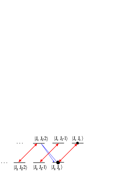
Figure 9: (Color online) Degenerate dipole transition $J_{g}\rightarrow J_{e}=J_{g}+1$ driven by $\sigma_{+}$-polarized light (thick red double arrows). In the notation of the ground and excited state sublevels, the first number refers to the angular momentum and the second one to the magnetic quantum number. The black dots show that the populations in the steady-state limit are distributed among the states $|J_{g}\,J_{g}\rangle$ and $|J_{e}\,J_{e}\rangle$, with $J_{e}=J_{g}+1$. The CBS signal in the helicity preserving channel appears due to the double scattering process on the transition between $|J_{g}\,J_{g}\rangle$ and $|J_{e}\,J_{e}\!-\!2\rangle$ depicted by the thin blue arrow.

In Fig. 9 we present a steady state population distribution for an atom with such a transition optically pumped by a $\sigma_{+}$-polarized laser field. Apart from that, in Fig. 9, we depict a scattering process which leads to a signal in the h $\parallel$ h polarization channel. This (double) scattering process is mediated by the excited state sublevel $|J_{e}\,J_{e}\!-\!2\rangle$ (we remind the reader that first and second symbol refer to the total angular momentum and to magnetic quantum number, respectively). In the linear scattering regime, the relevant levels are the three sublevels $|J_{e}\,J_{e}\!-\!2\rangle$, $|J_{g}\,J_{g}\rangle$, and $|J_{e}\,J_{e}\rangle$. Therefore, for any ground state angular momentum, the ground state degeneracy becomes immaterial, and perfect phase coherence of the CBS signal is predicted kupriyanov04 . Does this imply that, in the nonlinear scattering regime, the enhancement factor decays in the same way as it does for $J_{g}=0$ as a function of the laser field strength? As evident from Fig. 9, when two or more laser photons are involved in the scattering process, the state $|J_{e}\,J_{e}\!-\!2\rangle$ can be coupled to the ground state sublevel $|J_{g}\,J_{g}\!-\!2\rangle$ (if $J_{g}\geq 1$), such that the atom effectively becomes an N-type four-level system with the ground state sublevels $|J_{g}\,J_{g}\!-\!2\rangle$, $|J_{g}\,J_{g}\rangle$ and the excited state sublevels $|J_{e}\,J_{e}\!-\!2\rangle$, $|J_{e}\,J_{e}\rangle$. In this case, the ground state degeneracy does come into play even though the atoms are optically pumped. Below, we will explore the effect of the internal degeneracy in optically pumped atoms quantitatively, using the diagrammatic pump-probe approach.

IV.2 Selection of the polarization indices

The qualitative consideration of Sec. IV.1 allows us to identify all the polarization indices of the single-atom blocks in Figs. 6 and 7. We recall that the indices $r$, $r^{\prime}$ describe the incoming waves, and $q$, $q^{\prime}$ the outgoing ones; the index $q_{D}$ corresponds to the polarization of the detected signal.

Let us first consider the ladder contribution, see Fig. 6. It is easy to see that $q=q^{\prime}=+1$, since this corresponds to the polarization of the field radiated by an atom that is optically pumped by a $\sigma_{+}$-polarized laser field. Indices $r$, $r^{\prime}$ correspond to the $\sigma_{-}$-polarized probe field depicted by the thin blue arrow in Fig. 9, hence, $r=r^{\prime}=-1$. Finally, detection in the parallel helicity channel means that $q_{D}=-1$. As regards the crossed contribution, see Fig. 7, we likewise obtain, for diagram (C): $r^{\prime}=q_{D}=-1$, $q=+1$, and for diagram (D): $r=q_{D}=-1$, $q^{\prime}=+1$.

It follows from the above that, both, the ladder and crossed contributions are proportional to the geometric weight $\langle|\overleftrightarrow{\boldsymbol{\Delta}}_{-1,+1}|^{2}\rangle$, for any $J_{g}$. Using the definitions (9), (10), and (11), we easily perform the angular integrations to obtain $\langle|\overleftrightarrow{\boldsymbol{\Delta}}_{-1,+1}|^{2}\rangle=2/15$.

IV.3 Some basic properties of the building blocks for optically pumped atoms

With the polarization indices fixed, the elementary single-atom building blocks required for the evaluation of the double scattering signal in the h $\parallel$ h polarization channel can readily be evaluated using Eqs. (21) and (27). Some of these elementary blocks vanish identically in this channel, what reduces the total number of the double scattering diagrams. First, let us consider the elementary block shown in Fig. 8(a) (or its complex conjugate) with the downward-directed arrow. Indeed, the corresponding amplitude describes single scattering and must have the same polarization as the laser field. Its contribution therefore vanishes in the h $\parallel$ h polarization channel (where $q_{D}=-1$, as opposed to $q=q^{\prime}=+1$ for the incident laser). By the same argument, all double scattering diagrams containing the blocks (b1), (b2) (Fig. 6), (c2) and (d2) (Fig. 7) yield zero contribution. Second, let us examine the block (b4) in Fig. 6 which is composed of the two elementary blocks (see Fig. 8(c)) describing phase conjugation processes of the probe fields in the presence of the laser field shatokhin12a , whereupon the incoming solid arrow turns into the outgoing dashed arrow and vice versa. These are nonlinear transformations of the probe fields which can only take place if the probe and laser field polarizations coincide. But this is not the case in the helicity-preserving channel (where $r=r^{\prime}=-1$ and $q=q^{\prime}=+1$, see Sec. IV.2), hence, there is no contribution to the ladder spectrum due to the block (b4).

After excluding the diagrams that do not contribute in the h $\parallel$ h polarization channel, we end up with four double scattering diagrams contributing each to the ladder and to the crossed spectrum. We now consider the elastic and inelastic components of both spectra separately.

IV.4 Elastic component

The elastic ladder and crossed double scattering spectra are obtained by combining diagrams (a1) and (b3) in Fig. 6 and diagrams (c1) and (d1) in Fig. 7, respectively. It is evident that the resulting ladder and crossed diagrams contain the same elementary blocks. Hence, as expected kupriyanov04 , the elastic component of the double scattering contribution to CBS yields perfect interference contrast in the parallel helicity channel. We have phenomenologically deduced an analytical expression for these intensities which, as we have checked, exactly coincides with the result based on the numerical solution of the OBE (see above) for arbitrary choice of the parameters $\Omega$, $\delta$, and $J_{g}$:

$$L_{\rm el}=C_{\rm el}=\frac{1}{(4J_{g}+1)^{2}}\frac{1}{1+(\delta/\gamma)^{2}}\frac{s}{(1+s)^{4}},$$ (29)

where we dropped a common geometric prefactor, and introduced the saturation parameter

$$s=\frac{1}{2}\frac{\Omega^{2}}{\gamma^{2}+\delta^{2}}.$$ (30)

For $J_{g}=0$, Eq. (29) reduces to the result for Sr atoms derived using the master equation approach shatokhin05 .

As already noted, perfect interference contrast, following from Eq. (29), is a consequence of the optical pumping, whereupon the internal degeneracy does not play any role. In the opposite case of degenerate atoms in the thermal equilibrium (all ground state sublevels are equally populated), the contrast is in general $<1$, but its maximum value is restored in the semiclassical limit $J_{g}\to\infty$ cord_thesis .

IV.5 Inelastic spectrum

The sum of the remaining self-consistent combinations of diagrams: (a1)(b5) + (a2)(b3) + (a2)(b5) (see Fig. 6), yields inelastic ladder, and the sum (c1)(d3) + (c3)(d1) + (c3)(d3) (see Fig. 7) – inelastic crossed spectra. Below, we present our numerical results obtained by substituting solutions of Eqs. (21) and (27) into the above graphical equations, along with a qualitative discussion of how the internal degeneracy of optically pumped atoms affects the inelastic CBS spectra.

In the inelastic scattering regime, the laser field couples the excited state of the CBS transition to the unpopulated ground state sublevel with $m_{g}=J_{g}-2$ (see Fig. 9). Since such a coupling is impossible for atoms with $J_{g}=0$ and $J_{g}=1/2$, these two types of transitions are expected to exhibit similar behavior in the helicity preserving channel. And indeed, as our calculations show (Figs. 10(a), (b) and Fig. 12), the inelastic spectra for $J_{g}=1/2$ coincide, up to a prefactor $1/9=(4J_{g}+1)^{-2}$, with the double scattering spectra for the transition with $J_{g}=0$. Since the same prefactor appears in the expression for the elastic intensities, see Eq. (29), the enhancement factors must coincide for the transitions with $J_{g}=1/2$ and $J_{g}=0$, for arbitrary parameters of the laser field.

For atoms with $J_{g}\geq 1$, the CBS transition shares a common excited state with the laser-driven transition $|J_{g}\;J_{g}\!-\!2\rangle\leftrightarrow|J_{e}\;J_{e}\!-\!2\rangle$ (see Fig. 9), what leads to qualitatively different spectra in the weakly and strongly inelastic scattering regimes, as compared to the case of the non-degenerate atoms.

Below, we illustrate the above claims with numerical results for different values of $J_{g}$.

IV.5.1 Weakly inelastic scattering

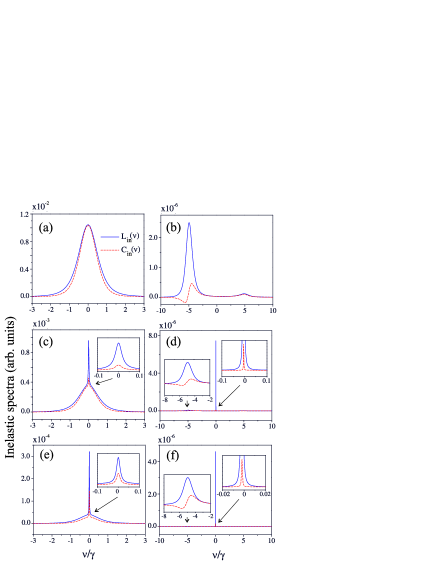
Figure 10: (color online) Inelastic ladder (solid) and crossed (dashed) double scattering CBS spectra in the weakly inelastic regime ($\Omega=0.3\gamma$), for four different dipole transitions. Top: $J_{g}=0$ and $J_{g}=1/2$. Both spectra coincide after rescaling the $J_{g}=1/2$ plots by the factor 1/9. Middle: $J_{g}=1$, bottom: $J_{g}=3$. Left column: Exact resonance, $\delta=0$; right column: Detuned driving, $\delta=5\gamma$. Insets magnify narrow resonances that emerge for $J_{g}\geq 1$, centered at the driving frequency for $\delta=0$, and slightly shifted towards a more pronounced sideband for $\delta\neq 0$. In cases (d) and (f), sidebands at $\delta=5\gamma$ exist, but are not resolved on this scale.

Figure 10 shows several examples of the spectra for the case $\Omega=0.3\gamma$. By virtue of Eq. (30), this corresponds to the weakly inelastic regime, $s\ll 1$, for arbitrary detunings $\delta$. The results for the transitions $J_{g}=0$ and $J_{g}=1/2$ coalesce in Fig. 10(a) and (b) after rescaling the $J_{g}=1/2$ signal with the prefactor $(4J_{g}+1)^{2}$, see our discussion above. In the resonant case (left panels), ladder and crossed spectra exhibit an inelastic Rayleigh peak with a width of the order of $\gamma$, centered at $\nu=0$; in the detuned case (right panels), both spectra contain two sidebands centered at $\nu=\pm\delta$. The detailed analytical and numerical results for double scattering spectra and a physical interpretation thereof were presented for the case of Sr atoms ($J_{g}=0$) in ralf11 ; shatokhin07 . We stress that, here and in Sec. IV.5.2 below, the double scattering CBS spectra for Sr atoms calculated using the master equation approach shatokhin07 coincide with the ones found within the diagrammatic pump-probe approach ralf11 .

Starting from $J_{g}=1$, both the ladder and crossed spectra exhibit, in addition to the spectrally wide features that are present in the case of $J_{g}=0$ and $J_{g}=1/2$, narrow resonances centered at the laser frequency, $\nu=0$ [in the detuned case, the position of the narrow resonance is slightly shifted towards a more pronounced sideband, see Figs. 10(d), (f)].

Subnatural linewidth resonances are typical for atoms with degenerate dipole transitions grison91 ; javanainen92 ; gao94a ; berman08 ; polder76 ; gao94b . Using the insights gained in these previous works, the emerging narrow peaks in the double scattering CBS spectra in the case $J_{g}\geq 1$ can straightforwardly be explained berman08 : Namely, since the system is optically pumped, an additional time scale, the finite life time of unpopulated magnetic ground state sublevels, emerges. Associated with this lifetime, optically pumped atoms acquire an effective subnatural width $\approx s\gamma$. This width shows up in the CBS spectra as an additional narrow peak centered near $\nu=0$, when a field scattered from another atom couples to the unpopulated ground state sublevel via a laser field (see Fig. 9).

We will see below in Sec. IV.5.2 that, in the double scattering spectral signal from atoms with $J_{g}\gg 1$, ultranarrow peaks can appear even in the strong saturation regime, $s\gg 1$. In that case, the physical origin of the narrow resonances is quantum interference between stimulated emission processes.

IV.5.2 Inelastic scattering from saturated atoms

Since saturation sets in for $s\gtrsim 1$, the narrow features in the CBS spectra then disappear (unless $J_{g}\gg 1$). The degeneracy of the Zeeman sublevels is lifted by the dynamic Stark effect, and the shape of the double scattering CBS spectra can be understood by analyzing the dressed state structure of the relevant dipole transitions of the atoms.

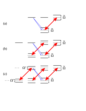
Figure 11: (color online) Dressed state structure for atoms with different ground state angular momenta (a) $J_{g}=0,$ (b) $J_{g}=1/2$, (c) $J_{g}\geq 1$. Modified Rabi frequency $\tilde{\Omega}=\sqrt{\Omega^{2}+\delta^{2}}$, and $\Omega^{\prime}$ is given by Eq. (31). While in cases (a) and (b) the structure of the levels relevant for double scattering is the same, in case (c) the excited state of the CBS transition is dressed by the laser field.

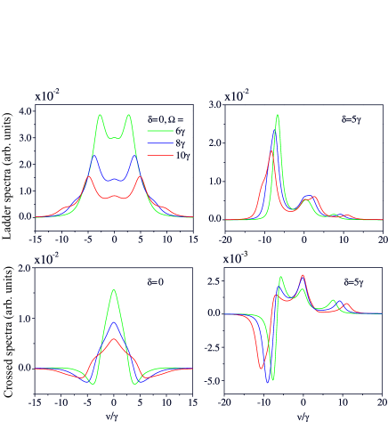
Figure 12: (color online) Examples of double scattering ladder (top) and crossed (bottom) spectra, for three different values of the Rabi frequency $\Omega$ (see legend) at resonance ($\delta=0$; left) and at a detuning $\delta=5\gamma$ (right), for $J_{g}=0$ and $J_{g}=1/2$. The spectra for both values of $J_{g}$ coalesce upon rescaling the $J_{g}=1/2$ spectra by a factor $(4J_{g}+1)^{-2}=1/9$.

Figure 11 schematically depicts the dressed levels of the optically pumped atoms with (a) $J_{g}=0$, (b) $J_{g}=1/2$, and (c) $J_{g}\geq 1$. In the former two cases, the structure of the dipole transition, relevant for the CBS signal in the h $\parallel$ h channel, is the same. Unsurprisingly, the ladder and crossed spectra for $J_{g}=0$ and $J_{g}=1/2$ plotted in Fig. 12 are identical, up to the numerical prefactor $1/9=(4J_{g}+1)^{-2}$ from Eq. (29). Note that, unlike Fig. 10, we present the ladder and crossed spectra in the saturation regime in separate plots – to facilitate the interpretation of the spectral features which become more complicated in this high intensity limit. Since the CBS spectra for Sr atoms have been discussed in detail in shatokhin07 , we right away move on to the case $J_{g}\geq 1$.

Results for the two examples $J_{g}=1$ and $J_{g}=3$ are presented in Fig. 13. As in the weakly inelastic regime, the spectra for $J_{g}\geq 1$ are different from those for $J_{g}<1$: Especially the number and the positions of the peaks differs. The main reason for this distinction in the saturation regime is a different dressed-state structure for $J_{g}\geq 1$ as compared to $J_{g}<1$, see Fig. 11.

In the limit of well-separated spectral lines, $\tilde{\Omega}\gg\gamma$, the splitting between the dressed levels corresponding to the transition $|J_{g}\,J_{g}\rangle\leftrightarrow|J_{e}\,J_{e}\rangle$ is equal to the modified Rabi frequency $\tilde{\Omega}=\sqrt{\Omega^{2}+\delta^{2}}$, whereas the splitting $\Omega^{\prime}$ between the dressed levels for the transition $|J_{g}\,J_{g}\!-\!2\rangle\leftrightarrow|J_{e}\,J_{e}\!-\!2\rangle$ is given by the product of the modified Rabi frequency and the corresponding Clebsch-Gordan coefficient,

$$\Omega^{\prime} =\tilde{\Omega}\langle J_{g}\,J_{g}\!\!-\!\!2,11|J_{g}\!\!+\!\!1\,J_{g}\!\!-\!\!1\rangle$$

$$=\tilde{\Omega}\sqrt{\frac{J_{g}(2J_{g}-1)}{2J_{g}^{2}+3J_{g}+1}}.$$ (31)

Due to these unequal splittings, there should appear four resonance frequencies in the CBS ladder spectra, which represent the various double scattering processes, at

$$\nu=\frac{1}{2}\left(\pm\tilde{\Omega}\pm\Omega^{\prime}\right).$$ (32)

Formula (32) describes accurately the positions of the resonances not only in the limit of well-separated spectral lines, but also for moderate values of the Rabi frequency. For instance, let us take $\delta=0$ and $\Omega=10\gamma$. In this case, the positions of the maxima of the ladder spectrum as obtained in Figs. 13(a) and (e) (red lines) from the solution of Eqs. (21) and (27) (with a binning size $0.1\gamma$ of the frequency axis) are (in units of $\gamma$):

$$\nu =\pm 2.8;\pm 7.1\;(J_{g}=1),$$

$$\nu =\pm 1.3;\pm 8.6\;(J_{g}=3).$$

In good agreement with these values, Eqs. (31) and (32) yield resonances centered at the frequencies

$$\nu =\pm 2.96;\pm 7.04\;(J_{g}=1),$$

$$\nu =\pm 1.34;\pm 8.66\;(J_{g}=3).$$

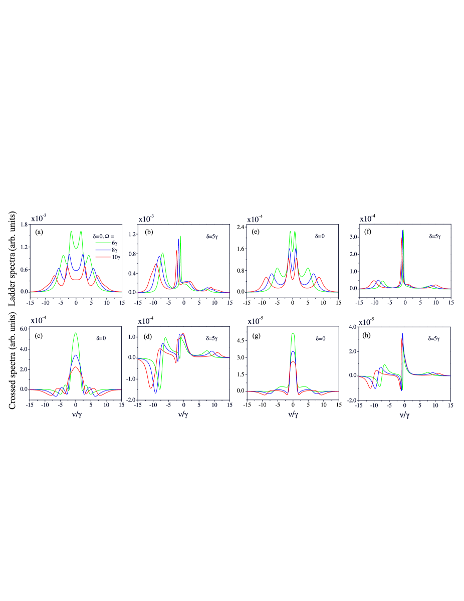
Figure 13: (color online) Examples of the double scattering ladder (top) and crossed (bottom) spectra, for three different values of the Rabi frequency $\Omega$ (see legend) for (a-d): $J_{g}=1$; and (e-h): $J_{g}=3$. Plots (a), (c), (e), and (g) are obtained at exact resonance, $\delta=0$, while (b), (d), (f), and (h) show the result for finite detuning, $\delta=5\gamma$.

As regards the crossed spectra, they originate from interferences between different inelastic scattering processes that are manifest in the ladder spectra as separate resonances shatokhin07 . These interferences lead to a peculiar line shape of the crossed spectra for $J_{g}=1$ and $J_{g}=3$ (see Fig. 13) which contains regions of, both, constructive and destructive interference, depending on the phase shifts associated with the corresponding frequency shifts upon inelastic scattering processes. Note that, in all cases, the maximum of the crossed spectrum occurs close to $\nu=0$. Therefore, the interference is always constructive close to the laser frequency.

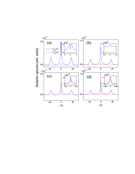
Figure 14: (color online) Inelastic ladder (solid) and crossed (dashed) double scattering CBS spectra at exact resonance ($\delta=0$) in the deep saturation regime ($\Omega=18\gamma$), for different dipole transitions: (a) $J_{g}=30$, (b) $J_{g}=110$, (c) $J_{g}=10^{3}$, and (d) $J_{g}=10^{4}$. Insets magnify narrow resonances.

It is interesting to study the double scattering spectra for larger values of $J_{g}$. In particular, this will allow us, in the next section, to answer the question of whether the CBS interference effect survives in the limit $J_{g}\to\infty$. Previously, it was established that a residual enhancement factor exists in the deep saturation regime for atoms with $J_{g}=0$ shatokhin05 , and in the elastic scattering regime for semiclassical atoms ($J_{g}\to\infty$) cord_thesis .

Using the aforementioned fact that optically pumped atoms with arbitrary $J_{g}$ can be modeled as effective few-level systems, it is possible to calculate the double scattering CBS spectra for arbitrary $J_{g}$ by simply readjusting the values of the Clebsch-Gordan coefficients. As we checked, these spectra look qualitatively the same as the spectra shown in Fig. 13, as long as $J_{g}\lesssim 40$. For larger values of $J_{g}$, the splitting $\Omega^{\prime}$ between the dressed levels converges to the modified Rabi frequency $\tilde{\Omega}$ (see Eq. (31)), and the two maxima of the ladder spectrum at $\nu=\pm(\tilde{\Omega}-\Omega^{\prime})/2$ merge. As a result, the ladder spectrum acquires a line shape consisting of three broad (linewidth $\sim\gamma$) peaks located at $\nu=-\tilde{\Omega},0,+\tilde{\Omega}$, and a subnatural linewidth peak at $\nu=0$, see Fig. 14. The three broad peaks represent nothing but the Mollow triplet mollow69 . It results from the spontaneous emission of the atom, excited by the probe field on the level $|J_{e}\,\,J_{e}\!-\!2\rangle$, down the dressed states of the CBS transition (which tends, for $J_{g}\gg 1$, to the dressed-state structure of the laser-driven two-level atom, see Fig. 11(c)). As for the narrow resonance, we believe that it originates from destructive interference between two stimulated emission processes from the dressed states, when $\nu\approx 0$ (leading to an extremely long lifetime of these states $\sim(J_{g}/\gamma)$). We deduce the linear scaling with $J_{g}$ from the observation of the behavior of the widths of the subnatural peaks which decrease as $\sim J_{g}^{-1}$ (see Fig. 14). Similar ultranarrow spectral features due to destructive interference between the dressed state transitions were predicted in resonance fluorescence of a four-level atom excited by a bichromatic coherent field zhu99 .

Concerning the crossed spectra, in the limit $J_{g}\gg 1$ it consists of a single positive narrow peak centered at $\nu=0$ (see Fig. 14). Its width coincides with the width of the narrow ladder resonance and, hence, it also decreases as $\sim J_{g}^{-1}$ with increasing $J_{g}$.

To see better how the above described spectral signatures affect the net interference effect of all the elastic and inelastic scattering processes, we conclude our study with an investigation of the total CBS enhancement factor, in the next section.

IV.6 Enhancement factor

The enhancement factor $\alpha$ is a quantitative measure of phase coherence between the interfering waves which contribute to the CBS signal. In the h $\parallel$ h channel, it is defined as jonckheere00

$$\alpha(\theta)=1+\frac{C_{\rm tot}(\theta)}{L_{\rm tot}},$$ (33)

where $\theta$ is the observation angle with respect to the backwards direction, and $C_{\rm tot}(\theta)$ and $L_{\rm tot}$ are the total crossed and ladder intensities of double scattering, respectively. Hereafter, we consider the exact backward direction, $\theta=0$.

In the inelastic scattering regime, the total intensities are given by the sums of the elastic and inelastic intensities

$$C_{\rm tot}(0) =C_{\rm el}+C_{\rm in},$$ (34)

$$L_{\rm tot} =L_{\rm el}+L_{\rm in},$$ (35)

where the elastic components, $C_{\rm el}=L_{\rm el}$, are defined in Eq. (29), and the inelastic intensities

$$C_{\rm in}=\int_{\infty}^{\infty}d\nu C_{\rm in}(\nu),\quad L_{\rm in}=\int_{\infty}^{\infty}d\nu L_{\rm in}(\nu),$$ (36)

are given by integrations over their frequency distributions.

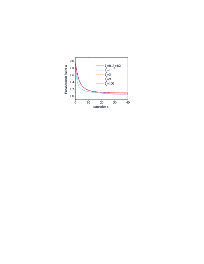
Figure 15: (color online) Coherent backscattering enhancement factor $\alpha$ vs. saturation $s$, at resonant driving, for different values of $J_{g}$. The enhancement factor initially decreases faster with increasing saturation for higher values of $J_{g}$.

Applying the formulas (33)-(36) to the calculated spectra, we study the behavior of the enhancement factor versus the saturation parameter, for different values of the ground state angular momenta. Our results for the case of exact resonance are presented in Fig. 15.

In the elastic scattering regime, that is for $s\to 0$, the enhancement factor features perfect phase coherence – $\alpha\to 2$ – for arbitrary $J_{g}$. This is in full agreement with our result for the elastic ladder and crossed intensities, see Eq. (29). Furthermore, the results for $J_{g}=0$ and $J_{g}=1/2$ coincide for all $s$. As already discussed in Sec. IV.5, the ground state degeneracy does not affect the phase coherence in these cases; the decrease of $\alpha$ is due to inelastic scattering processes alone.

Starting from $J_{g}=1$, the enhancement factor exhibits an initially steeper decay of $\alpha$ with $s$ as $J_{g}$ increases. We attribute this behavior to the fact that the coupling of the excited state $|J_{e}\,J_{e}\!-\!2\rangle$ to the ground state $|J_{g}\,J_{g}\!-\!2\rangle$ increases with $J_{g}$, due to the growth of the associated Clebsch-Gordan coefficients. Although, at intermediate and large values of $s$, larger values of $J_{g}$ do not necessarily lead to a faster decrease of $\alpha$ with $s$, the result for $J_{g}=0$ and $J_{g}=1/2$ yields an upper bound. In other words, when the internal degeneracy comes into play, it always leads to a faster decay of the phase coherence as compared to the non-degenerate case.

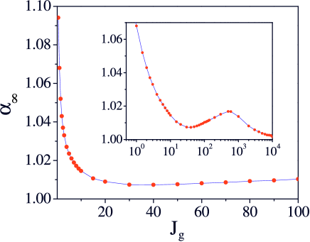
Figure 16: (color online) Residual enhancement factor $\alpha_{\infty}$ at $s=162\gg 1$, versus $J_{g}=0$, 1/2, 1, 3/2, 2, 5/2, 3, 4, 5, 6, 7, 8, 9, 10, 15, etc, with $\alpha_{\infty}(0)=\alpha_{\infty}(1/2)\approx 1.095$. Inset: semi-log graph of $\alpha_{\infty}(J_{g})$, with $\alpha_{\infty}(10^{4})\approx 1.0016$. The continuous line guides the eye.

Finally, let us discuss the asymptotic behavior of the enhancement factor $\alpha_{\infty}$ in the deep saturation regime, $s\gg 1$. For double scattering from Sr atoms, we found earlier that the inelastic ladder and crossed intensities asymptotically decrease as $\sim s^{-1}$, leading to a residual enhancement $\alpha_{\infty}\approx 1.095$ in the case of resonant driving shatokhin05 . The dependence of $\alpha_{\infty}$ on $J_{g}$ is presented in Fig. 16. For $J_{g}>1/2$, $\alpha_{\infty}$ drops with increasing total angular momentum, until it reaches a minimum of $\alpha_{\infty}(40)\approx 1.0073$. Further increase of $J_{g}$ leads to a very slow but monotonous increase of the residual enhancement until $J_{g}\approx 500$, where a local maximum of $\alpha_{\infty}(500)\approx 1.017$ is reached (see inset in Fig. 16). This behavior is unsurprising when taking into account that the increase in $J_{g}$ is not accompanied by an increase in the effective internal ground state degeneracy, which remains equal to 2 for any $J_{g}\geq 1$. The slow growth of $\alpha_{\infty}$ for $J_{g}>40$ can be attributed to the fact that the total weight of the ladder spectrum decreases after merging two central peaks into one single peak (see Fig. 14(a) and (b)).

Further increase of $J_{g}$ leads to a monotonous decrease of $\alpha_{\infty}$. As follows from the discussion in Sec. IV.5.2 and Fig. 14, for very large values of $J_{g}$, an increase of $J_{g}$ is accompanied by narrowing of the subnatural linewidth resonances of the ladder and crossed spectra, without affecting the broad spectral features of the ladder spectra. This is not compensated by an increase of the relative peaks’ heights, which remain fixed for a given value of $s$. Therefore, we predict that the enhancement factor should asymptotically tend to unity:

$$\alpha_{\infty}=1+O(J_{g}^{-1}),\quad J_{g}\to\infty.$$ (37)

V Summary and Conclusion

In this work, we generalized the pump-probe approach to CBS of light by cold two-level atoms geiger10 ; wellens10 ; shatokhin12a to atoms with degenerate energy levels. For this, we derived equations of motion for a generalized Bloch vector, describing the dynamics of a single atom under a classical bichromatic driving field. Because these equations are formally equivalent to the equations appearing in the pump-probe approach for two-level atoms, we could translate our equations to the same diagrammatic language. By doing so, we obtained similar single-atom building blocks as in shatokhin12a , where, in the generalized diagrams, each incoming and outgoing arrow is additionally equipped with a polarization index. Like for two-level atoms, the double scattering contributions to CBS can be derived by combining these single-atom building-blocks self-consistently.

We applied the generalized pump-probe approach to study double scattering from optically pumped atoms in the helicity preserving polarization channel. To this end, we considered several examples of the dipole transition $J_{g}\rightarrow J_{e}=J_{g}+1$. Comparing our results for the $J_{g}=0$ transition with the master equation results shatokhin05 ; shatokhin07 , for different parameter values, we could establish perfect agreement between both approaches.

For $J_{g}\geq 1$, the internal degeneracy manifests itself in the inelastic scattering signal, leading to a faster decay of the CBS enhancement factor with increasing saturation of the atomic transition as compared to the non-degenerate case. Finally, we predict that, in the deep saturation regime, the CBS interference signal should asymptotically vanish with increasing $J_{g}$, as $J_{g}^{-1}$.

Appendix A Projecting vectors

For a dipole transition with the ground and excited state angular momenta $J_{g}$ and $J_{e}$, respectively, the complete orthogonal basis set contains $N=(2(J_{e}+J_{g})+2)^{2}-1$ operators. We denote these operators by $\mu_{1},\ldots,\mu_{N}$. Consequently, the generalized optical Bloch vector can be written as

$${\bf Q}=(\mu_{1},\ldots,\mu_{N})^{T},$$ (38)

where $T$ denotes transposition. Among these operators, it is convenient to choose the first $N_{0}=2(J_{e}+J_{g})+2$ operators as the identity operator and $N_{0}-1$ diagonal traceless operators. The remaining $N-N_{0}$ operators are chosen as non-diagonal operators describing transitions between pairs of different sublevels. Then, the set of operators $\mu^{\prime}_{i}$, orthogonal to the set of operators $\mu_{i}$, can be chosen in the following way: The first $N_{0}$ operators of the orthogonal set read $\mu^{\prime}_{i}=\mu_{i}/{\rm Tr}[\mu_{i}^{2}]$ ($i=1,\ldots,N_{0}$), and the remaining operators $\mu_{i}^{\prime}=\mu_{i}^{T}$.

It is easy to see that, in this case, the orthogonality condition, ${\rm Tr}[\mu_{n}\mu_{m}^{\prime}]=\delta_{nm}$, is fulfilled for all $1\leq n,m\leq N$. Consequently, any operator ${\cal O}=\sum_{i}c_{i}\mu_{i}$ can be defined as a scalar product

$${\cal O}={\bf C}\cdot{\bf Q},\quad\langle{\cal O}\rangle={\bf C}\cdot\langle{\bf Q}\rangle,$$ (39)

where ${\bf C}=(c_{1},\ldots,c_{N})$ is a projecting vector, with $c_{i}={\rm Tr}[{\cal O}\mu_{i}^{\prime}]$. Likewise, we denote the vectors projecting onto the operator $D_{q}^{\dagger}$ and $D_{q}$ to be ${\bf U}_{q}$ and ${\bf V}_{q}$, respectively:

$$\langle D_{q}^{\dagger}\rangle={\bf U}_{q}\cdot\langle{\bf Q}\rangle,\quad\langle D_{q}\rangle={\bf V}_{q}\cdot\langle{\bf Q}\rangle.$$ (40)

Appendix B Initial conditions

We now explain how to define the initial conditions in Eq. (26). From the definitions of the correlation functions (27), we have

$${\bf f}_{q}(0) =\langle{\bf Q}D_{q}\rangle-\langle{\bf Q}\rangle\langle D_{q}\rangle,$$ (41a)

$${\bf h}_{q^{\prime}}(0) =\langle D^{\dagger}_{q^{\prime}}{\bf Q}\rangle-\langle D^{\dagger}_{q^{\prime}}\rangle\langle{\bf Q}\rangle,$$ (41b)

where the average should be taken with respect to the steady state of a single laser driven atom. We note that the perturbative expansion of the factorized part of the correlation function in Eq. (41) can be obtained directly from Eq. (21d). As regards the non-factorized parts on the right hand sides of (41), they can be expressed using Eq. (21d) as follows

$$\langle{\bf Q}D_{q}\rangle ={\bf A}_{1}\langle{\bf Q}\rangle+{\bf L}_{1},$$ (42a)

$$\langle D^{\dagger}_{q^{\prime}}{\bf Q}\rangle ={\bf A}_{2}\langle{\bf Q}\rangle+{\bf L}_{2},$$ (42b)

where

$$({\bf A}_{1})_{ij} ={\rm Tr}[\mu_{i}D_{q}\mu^{\prime}_{j}],\quad({\bf L}_{1})_{i}={\rm Tr}[D_{q}\mu^{\prime}_{i}]/N_{0},$$ (43a)

$$({\bf A}_{2})_{ij} ={\rm Tr}[D^{\dagger}_{q^{\prime}}\mu_{i}\mu^{\prime}_{j}],\quad({\bf L}_{2})_{i}={\rm Tr}[D^{\dagger}_{q^{\prime}}\mu^{\prime}_{i}]/N_{0}.$$ (43b)

Performing the perturbative expansion of both sides of Eq. (41a) to second order in the probe field, we obtain:

$${\bf f}^{(0)}_{q}(0) ={\bf A}_{1}\langle{\bf Q}\rangle^{(0)}+{\bf L}_{1}-\langle{\bf Q}\rangle^{(0)}\langle D_{q}\rangle^{(0)},$$ (44a)

$${\bf f}^{(+)}_{q}(\omega^{[r^{\prime}]};0) ={\bf A}_{1}\langle{\bf Q}(\omega^{[r^{\prime}]})\rangle^{(+)}-\langle{\bf Q}(\omega^{[r^{\prime}]})\rangle^{(+)}\langle D_{q}\rangle^{(0)}-\langle{\bf Q}\rangle^{(0)}\langle D_{q}(\omega^{[r^{\prime}]})\rangle^{(+)},$$ (44b)

$${\bf f}^{(-)}_{q}(\omega^{[r]};0) ={\bf A}_{1}\langle{\bf Q}(\omega^{[r]})\rangle^{(-)}-\langle{\bf Q}(\omega^{[r]})\rangle^{(-)}\langle D_{q}\rangle^{(0)}-\langle{\bf Q}\rangle^{(0)}\langle D_{q}(\omega^{[r]})\rangle^{(-)},$$ (44c)

$${\bf f}_{q}^{(+-)}(\omega^{[r^{\prime}]},\omega^{[r]};0) ={\bf A}_{1}\langle{\bf Q}(\omega^{[r^{\prime}]},\omega^{[r]})\rangle^{(+-)}-\langle{\bf Q}(\omega^{[r^{\prime}]},\omega^{[r]})\rangle^{(+-)}\langle D_{q}\rangle^{(0)}$$

$$-\langle{\bf Q}\rangle^{(0)}\langle D_{q}(\omega^{[r^{\prime}]},\omega^{[r]})\rangle^{(+-)}-\langle{\bf Q}(\omega^{[r^{\prime}]})\rangle^{(+)}\langle D_{q}(\omega^{[r]})\rangle^{(-)}$$

$$-\langle{\bf Q}(\omega^{[r]})\rangle^{(-)}\langle D_{q}(\omega^{[r^{\prime}]})\rangle^{(+)}.$$ (44d)

Expanding, in the same way, Eq. (41b) leads to the initial conditions for the vector ${\bf h}_{q^{\prime}}(0)$:

$${\bf h}^{(0)}_{q^{\prime}}(0) ={\bf A}_{2}\langle{\bf Q}\rangle^{(0)}+{\bf L}_{2}-\langle{\bf Q}\rangle^{(0)}\langle D^{\dagger}_{q^{\prime}}\rangle^{(0)},$$ (45a)

$${\bf h}^{(+)}_{q^{\prime}}(\omega^{[r^{\prime}]};0) ={\bf A}_{2}\langle{\bf Q}(\omega^{[r^{\prime}]})\rangle^{(+)}-\langle{\bf Q}(\omega^{[r^{\prime}]})\rangle^{(+)}\langle D^{\dagger}_{q^{\prime}}\rangle^{(0)}-\langle{\bf Q}\rangle^{(0)}\langle D^{\dagger}_{q^{\prime}}(\omega^{[r^{\prime}]})\rangle^{(+)},$$ (45b)

$${\bf h}^{(-)}_{q^{\prime}}(\omega^{[r]};0) ={\bf A}_{2}\langle{\bf Q}(\omega^{[r]})\rangle^{(-)}-\langle{\bf Q}(\omega^{[r]})\rangle^{(-)}\langle D^{\dagger}_{q^{\prime}}\rangle^{(0)}-\langle{\bf Q}\rangle^{(0)}\langle D^{\dagger}_{q^{\prime}}(\omega^{[r]})\rangle^{(-)},$$ (45c)

$${\bf h}_{q^{\prime}}^{(+-)}(\omega^{[r^{\prime}]},\omega^{[r]};0) ={\bf A}_{2}\langle{\bf Q}(\omega^{[r^{\prime}]},\omega^{[r]})\rangle^{(+-)}-\langle{\bf Q}(\omega^{[r^{\prime}]},\omega^{[r]})\rangle^{(+-)}\langle D^{\dagger}_{q^{\prime}}\rangle^{(0)}$$

$$-\langle{\bf Q}\rangle^{(0)}\langle D^{\dagger}_{q^{\prime}}(\omega^{[r^{\prime}]},\omega^{[r]})\rangle^{(+-)}-\langle{\bf Q}(\omega^{[r^{\prime}]})\rangle^{(+)}\langle D^{\dagger}_{q^{\prime}}(\omega^{[r]})\rangle^{(-)}$$

$$-\langle{\bf Q}(\omega^{[r]})\rangle^{(-)}\langle D^{\dagger}_{q^{\prime}}(\omega^{[r^{\prime}]})\rangle^{(+)}.$$ (45d)

References

- (1) A. Lagendijk and B. A. van Tiggelen, Phys. Rep. 270, 143, (1996).
- (2) P. Sheng, Introduction to Wave Scattering, Localization and Mesoscopic Phenomena (Academic Press, San Diego, 1995).
- (3) M. P. Van Albada and A. Lagendijk, Phys. Rev. Lett. 55, 2692 (1985); P.-E. Wolf and G. Maret, Phys. Rev. Lett. 55, 2696 (1985); Y. Kuga and A. Ishimaru, J. Opt. Soc. Am. A 1, 831 (1984).
- (4) G. Bayer and T. Niederdränk, Phys. Rev. Lett. 70, 3884 (1993); A. Tourin, A. Derode, P. Roux, B. A. van Tiggelen, and M. Fink, Phys. Rev. Lett. 79, 3637 (1997).
- (5) E. Larose, L. Margerin, B. A. van Tiggelen, and M. Campillo, Phys. Rev. Lett. 93, 048501 (2004).
- (6) F. Jendrzejewski, K. Müller, J. Richard, A. Date, T. Plisson, P. Bouyer, A. Aspect, and V. Josse, Phys. Rev. Lett. 109, 195302 (2012); G. Labeyrie, T. Karpiuk, J.-T. Schaff, B. Grémaud, and D. Delande, Europhys. Lett. 100, 66001 (2012).
- (7) G. Labeyrie, F. de Tomasi, J.-C. Bernard, C. A. Müller, C. Miniatura, and R. Kaiser, Phys. Rev. Lett. 83, 5266 (1999).
- (8) C. Cohen-Tannoudji, J. Dupont-Roc, and G. Grynberg, Atom-Photon Interactions, Chapter V (Wiley-VCH, Weinheim, 2004).
- (9) T. Chanelière, D. Wilkowski, Y. Bidel, R. Kaiser, and C. Miniatura, Phys. Rev. E 70, 036602 (2004).
- (10) S. Balik, P. Kulatunga, C. I. Sukenik, M. D. Havey, D. V. Kupriyanov, and I. M. Sokolov, J. Mod. Opt. 52, 2269 (2005).
- (11) T. Wellens, B. Grémaud, D. Delande, and C. Miniatura, Phys. Rev. A 70, 023817 (2004).
- (12) V. Shatokhin, C. A. Müller, and A. Buchleitner, Phys. Rev. Lett. 94, 043603 (2005); Phys. Rev. A 73, 063813 (2006).
- (13) B. Grémaud, T. Wellens, D. Delande, C. Miniatura, Phys. Rev. A 74, 033808 (2006).
- (14) T. Geiger, T. Wellens, V. Shatokhin, and A. Buchleitner, Photon. Nanostr. Fund. Appl. 8, 244 (2010).
- (15) T. Wellens, T. Geiger, V. Shatokhin, and A. Buchleitner, Phys. Rev. A 82, 013832 (2010).
- (16) P. Meystre, and M. Sargent, Elements of Quantum Optics (Springer Berlin, 2007) Chapter 9.
- (17) T. Binninger; Multiple Scattering of Intense Laser Light in a Cloud of Cold Atoms, Diploma Thesis (Albert-Ludwigs Universität Freiburg, 2012); www.freidok.uni-freiburg.de/volltexte/8812
- (18) V. Shatokhin, T. Geiger, T. Wellens, and A. Buchleitner, Chem. Phys. 375, 150 (2010).
- (19) V. Shatokhin and T. Wellens, Phys. Rev. A 86, 043808 (2012).
- (20) B. R. Mollow, Phys. Rev. 5, 2217 (1972).
- (21) R. Guccione-Gush and H. P. Gush, Phys. Rev. A 10, 1474 (1974).
- (22) G. S. Agarwal and N. Nayak, Phys. Rev. A 33, 391 (1986).
- (23) H. J. Kimble, M. Dagenais, and L. Mandel, Phys. Rev. Lett. 39, 691 (1977).
- (24) V. Shatokhin, T. Wellens, and A. Buchleitner, J. Phys. B 39, 4719 (2012).
- (25) T. Geiger, New approach to multiple scattering of intense laser light from cold atoms, Diploma Thesis (Albert-Ludwigs Universität Freiburg, 2009); www.freidok.uni-freiburg.de/volltexte/6986
- (26) R. W. Boyd, Nonlinear Optics, 2nd Edn. (San Diego, CA: Academic) Chapter 6.
- (27) T. Wellens and B. Grémaud, Phys. Rev. Lett. 100, 033902 (2008).
- (28) V. Shatokhin, T. Wellens, B. Grémaud, and A. Buchleitner, Phys. Rev. A 76, 043832 (2007).
- (29) R. Blattmann, The pump-probe approach to coherent backscattering of intense laser light by cold atoms with degenerate energy levels, Diploma Thesis (Albert-Ludwigs Universität Freiburg, 2011); www.freidok.uni-freiburg.de/volltexte/9185
- (30) G. Labeyrie, D. Delande, C. A. Müller, C. Miniatura, and R. Kaiser, Europhys. Lett. 61, 327 (2003).
- (31) D. V. Kupriyanov, I. M. Sokolov, C. I. Sukenik and M. D. Havey, Laser Phys. Lett. 3, 223 (2006).
- (32) J. J. Sakurai, Modern Quantum Mechanics (Addison-Wesley Publishing Company, 1994) Revised Edn., Chapter 3.
- (33) T. Jonckheere, C. A. Müller, R. Kaiser, C. Miniatura and D. Delande, Phys. Rev. Lett. 85 4269 (2000).
- (34) C. A. Müller and C. Miniatura, J. Phys. A 35, 10163 (2002).
- (35) D. V. Kupriyanov, I. M. Sokolov, P. Kulatunga, C. I. Sukenik and M. D. Havey, Phys. Rev. A 67, 013814 (2003).
- (36) G. Grynberg, A. Aspect, and C. Fabre, Introduction to Quantum Optics. From the Semi-Classical Approach to Quantized Light (Cambridge University Press, New York, 2010) Complement 2B.
- (37) Bo Gao, Phys. Rev. A 48, 2443 (1993).
- (38) D. V. Kupriyanov, I. M. Sokolov, N. V. Larionov, P. Kulatunga, C. I. Sukenik, S. Balik, and M. D. Havey, Phys. Rev. A 69, 033801 (2004).
- (39) C. A. Müller, Localisation faible de la lumière dans un gaz d’atomes froids: rétrodiffusion cohérente et structure quantique interne, PhD Thesis (LMU, München, 2001); http://edoc.ub.uni-muenchen.de/400/
- (40) D. Grison, B. Lounis, C. Salomon, J. Y. Courtois, and G. Grynberg, Europhys. Lett. 15, 149 (1991); J. W. R. Tabosa, G. Chen, Z. Hu, R. B. Lee, and H. J. Kimble, Phys. Rev. Lett. 66, 3245 (1991).
- (41) J. Javananainen, Europhys. Lett. 20, 395 (1992).
- (42) Bo Gao, Phys. Rev. A 49, 3391 (1994).
- (43) P. R. Berman, Contemp. Phys. 49, 313 (2008).
- (44) D. Polder and M. F. H. Schuurmans, Phys. Rev. A 14, 1468 (1976).
- (45) Bo Gao, Phys. Rev. A 50, 4139 (1994).
- (46) B. R. Mollow, Phys. Rev. 188, 1969 (1969).
- (47) Fu-li Li and Shi-Yao Zhu, Phys. Rev. A 59, 2330 (1999).