Refined curve counting with tropical geometry

Abstract.

The Severi degree is the degree of the Severi variety parametrizing plane curves of degree $d$ with $\delta$ nodes. Recently, Göttsche and Shende gave two refinements of Severi degrees, polynomials in a variable $y$, which are conjecturally equal, for large $d$. At $y=1$, one of the refinements, the relative Severi degree, specializes to the (non-relative) Severi degree.

We give a tropical description of the refined Severi degrees, in terms of a refined tropical curve count for all toric surfaces. We also refine the equivalent count of floor diagrams for Hirzebruch and rational ruled surfaces. Our description implies that, for fixed $\delta$, the refined Severi degrees are polynomials in $d$ and $y$, for large $d$. As a consequence, we show that, for $\delta\leq 10$ and all $d$, both refinements of Göttsche and Shende agree and equal our refined counts of tropical curves and floor diagrams.

1. Introduction

A $\delta$-nodal curve is a reduced (not necessarily irreducible) curve with $\delta$ simple nodes and no other singularities. The Severi degree $N^{d,\delta}$ is the degree of the Severi variety parametrizing plane $\delta$-nodal curves of degree $d$. Equivalently, $N^{d,\delta}$ is the number of $\delta$-nodal plane curves of degree $d$ through $\tfrac{(d+3)d}{2}-\delta$ generic points in the complex projective plane ${\mathbb{P}}^{2}$.

Severi degrees are generally difficult to compute. Their study goes back to the midst of 19th century, when Steiner [24], in 1848, showed that the degree $N^{d,1}$ of the discriminant of ${\mathbb{P}}^{2}$ is $3(d-1)^{2}$. Only in 1998, Caporaso and Harris [8] computed $N^{d,\delta}$ for any $d$ and $\delta$, by their celebrated recursion (involving relative Severi degrees $N^{d,\delta}(\alpha,\beta)$ counting curves satisfying tangency conditions to a fixed line).

Di Francesco and Itzykson [9], in 1994, conjectured the numbers $N^{d,\delta}$ to be polynomial in $d$, for fixed $\delta$ and $d$ large enough. In 2009, Fomin-Mikhalkin [10] showed that, for each $\delta\geq 1$, there is a polynomial $N_{\delta}(d)$ in $d$ with $N^{d,\delta}=N_{\delta}(d)$, provided that $d\geq 2\delta$. The polynomials $N_{\delta}(d)$ are called node polynomials.

More generally, for $S$ a projective algebraic surface, and $L$ a line bundle on $S$, the Severi degree $N^{(S,L),\delta}$ is the number of $\delta$-nodal curves in the complete linear system $|L|$ through $\dim|L|-\delta$ general points of $S$ . In [13] it was conjectured that the Severi degrees of arbitrary smooth projective surfaces $S$ with a sufficiently ample line bundle $L$ are given by universal polynomials. Specifically the conjecture predicts for each fixed $\delta$, the existence of a polynomial $\widetilde{N}^{(S,L),\delta}$ in the intersection numbers $L^{2}$, $LK_{S}$, $K_{S}^{2}$, $c_{2}(S)$ such that $N^{(S,L),\delta}=\widetilde{N}^{(S,L),\delta}$ for $L$ sufficiently ample. We call the $\widetilde{N}^{(S,L),\delta}$ the curve counting invariants. In addition the $\widetilde{N}^{(S,L),\delta}$ were conjectured to be given by a multiplicative generating function, i.e. there are universal power series $A_{1},A_{2},A_{3},A_{4}\in{\mathbb{Q}}[[q]]$, such that

(1.1) $$\sum_{\delta\geq 0}\widetilde{N}^{(S,L),\delta}q^{\delta}=A_{1}^{L^{2}}A_{1}^{LK_{S}}A_{3}^{K_{S}^{2}}A_{4}^{c_{2}(S)}.$$

Furthermore $A_{1}$ and $A_{2}$ are given explicitly in terms of modular forms. This conjecture was proved by Tzeng [25] in 2010. A second proof was given shortly afterwards by Kool, Shende, and Thomas [19]. In the latter proof, the authors identified the numbers $\widetilde{N}^{(S,L),\delta}$ as coefficients of the generating function of the topological Euler characteristics of relative Hilbert schemes (see Section 2). This is motivated by the proposed definition the Gopakumar Vafa (BPS) invariants in terms of Pandharipande-Thomas invariants in [21]. Thus the curve counting invariants can be viewed as special cases of BPS invariants. By definition for $S={\mathbb{P}}^{2}$ and $L={\mathcal{O}}(d)$, the curve counting invariants coincide with the node polynomials: $\widetilde{N}^{({\mathbb{P}}^{2},{\mathcal{O}}(d)),\delta}=N_{\delta}(d)$.

Inspired by this description, in [14] refined invariants $\widetilde{N}^{(S,L),\delta}(y)$ are defined as coefficients of a very similar generating function, but with the topological Euler characteristic replaced by the normalized $\chi_{-y}$-genus, a specialization of the Hodge polynomial. They are Laurent polynomials in $y$, symmetric under $y\mapsto\frac{1}{y}$. In [14] a number of conjectures are made about the refined invariants $\widetilde{N}^{(S,L),\delta}(y)$. In particular they are conjectured to have a multiplicative generating function (as in (1.1)), where now two of the universal power series are explicitly given in terms of Jacobi forms. This fact was proven in the meantime in [15] in case the canonical divisor $K_{S}$ is numerically trivial.

In this paper we will concentrate on the case that $S$ is a toric surface, and sometimes we restrict to the case that $S={\mathbb{P}}^{2}$, $L={\mathcal{O}}(d)$, and denote $\widetilde{N}^{({\mathbb{P}}^{2},{\mathcal{O}}(d)),\delta}(y)=\widetilde{N}^{d,\delta}(y)$. In the case that $S$ is a toric surface and $L$ a toric line bundle, we will change slightly the definition of the Severi degrees. We denote $N^{(S,L),\delta}$ the number of cogenus $\delta$ curves in $|L|$ passing though $\dim|L|-\delta$ general points in $S$, which do not contain a toric boundary divisor as a component. This is done because, as we will see below, with this new definition (and not with the old one) the Severi degrees can be computed via tropical geometry and by a Caporaso-Harris type recursion formula. The Severi degrees as defined before we denote by $N_{*}^{(S,L),\delta}$, but we will not consider them in the sequel.

If $L$ is $\delta$-very ample (see below for the definition) it is easy to see (Remark 2.1) that $N^{(S,L),\delta}=N^{(S,L),\delta}_{*}$. In case $S={\mathbb{P}}^{2}$ it is easy to see that $N^{d,\delta}=N^{d,\delta}_{*}$. By definition the Caporaso-Harris type recursion of [8], [26] always computes the invariants $N^{(S,L),\delta}$ for ${\mathbb{P}}^{2}$ and rational ruled surfaces.

If $S$ is ${\mathbb{P}}^{2}$ or a rational ruled surface, in [14] refined Severi degrees $N^{(S,L),\delta}(y)$ are defined by a modification of the Caporaso-Harris recursion. These are again Laurent polynomials in $y$, symmetric under $y\mapsto\frac{1}{y}$. Again, in the case of ${\mathbb{P}}^{2}$, we denote the refined Severi degrees by $N^{d,\delta}(y)$. The recursion specializes to that [8], [26] at $y=1$, so that $N^{(S,L),\delta}(1)=N^{(S,L),\delta}$.

In this paper we will relate the refined Severi degrees $N^{(S,L),\delta}(y)$ and $N^{d,\delta}(y)$ to tropical geometry. Mikhalkin [20] has shown that the Severi degrees of projective toric surfaces can be computed by toric geometry. Fix a lattice polygon $\Delta$ in ${\mathbb{R}}^{2}$, i.e. $\Delta$ is the convex hull of a finite subset of ${\mathbb{Z}}^{2}$. Then $\Delta$ determines via its normal fan a projective toric surface $X(\Delta)$ and an ample line bundle $L=L(\Delta)$ on $X(\Delta)$ (and $H^{0}(X(\Delta),L(\Delta))$ can be identified with the vector space with basis $\Delta\cap{\mathbb{Z}}^{2}$). Conversely a pair $(X,L)$ of a toric surface and a line bundle on $X$ determines a lattice polygon. We denote by $N^{\Delta,\delta}$ the number of (possibly reducible) cogenus $\delta$ curves of degree $\Delta$ in $({\mathbb{C}}^{*})^{2}$ passing through $|\Delta\cap{\mathbb{Z}}^{2}|-1-\delta$ general points, as defined in [20, Def. 5.1]. By definition $N^{(X(\Delta),L(\Delta)),\delta}=N^{\Delta,\delta}$. The invariants $N^{\Delta,\delta}$ can be computed in tropical geometry.

If $X(\Delta)$ is ${\mathbb{P}}^{2}$ or a rational ruled surface, we will in the future also write $N^{\Delta,\delta}(y):=N^{(X(\Delta),L(\Delta)),\delta}(y)$ for the corresponding (refined) Severi degrees as defined in [14]. By our definition we then have $N^{\Delta,\delta}(1)=N^{\Delta,\delta}$.

In tropical geometry the Severi degrees $N^{\Delta,\delta}$ can be computed as the count of simple tropical curves $C$ in ${\mathbb{R}}^{2}$ through $\dim|L(\Delta)|-\delta$ general points, counted with certain multiplicities $\operatorname{mult}_{\mathbb{C}}(C)$. Roughly speaking, a simple tropical curve is a trivalent graph $C$ immersed in ${\mathbb{R}}^{2}$, with some extra data. From this data, one assigns to each vertex $v$ of $C$ a multiplicity $\operatorname{mult}_{\mathbb{C}}(v)$, and defines the multiplicity $\operatorname{mult}_{\mathbb{C}}(C)$ as the product $\prod_{v\ \text{vertex of }C}\operatorname{mult}_{\mathbb{C}}(v)$.

For any integer $n$, and a variable $y$, we introduce the quantum number $[n]_{y}$ by

(1.2) $$[n]_{y}=\frac{y^{n/2}-y^{-n/2}}{y^{1/2}-y^{-1/2}}=y^{(n-1)/2}+\cdots+y^{-(n-1)/2}.$$

By definition $[n]_{1}=n$. We introduce a new polynomial multiplicity $\operatorname{mult}(C;y)\in{\mathbb{Z}}_{\geq 0}[y^{1/2},y^{-1/2}]$ for tropical curves by $\operatorname{mult}(C;y)=\prod_{v\ \text{vertex of }C}[\operatorname{mult}_{\mathbb{C}}(v)]_{y}$, and define the tropical refined Severi degrees $N^{\Delta,\delta}_{\text{trop}}(y)$ as the count of simple tropical curves $C$ in ${\mathbb{R}}^{2}$ through $\dim|L(\Delta)|-\delta$ general points with multiplicity $\operatorname{mult}(C;y)$. By definition $N^{\Delta,\delta}_{\text{trop}}(y)\in{\mathbb{Z}}_{\geq 0}[y^{1/2},y^{-1/2}]$. By definition $[\operatorname{mult}_{\mathbb{C}}(v)]_{1}=\operatorname{mult}_{\mathbb{C}}(v)$, thus we see that $N^{\Delta,\delta}_{\text{trop}}(1)=N^{\Delta,\delta}$.

A priori, $N^{\Delta,\delta}_{\text{trop}}(y)$ should depend on a configuration $\Pi$ of $\dim|L(\Delta)|-\delta$ general points in ${\mathbb{R}}^{2}$ but Itenberg and Mikhalkin show in [17] that $N^{\Delta,\delta}_{\text{trop}}(y)$ is a tropical invariant, i.e. independent of $\Pi$.

We will prove that in the case of the plane and rational ruled surfaces, when the refined Severi degrees have been defined in [14], they equal the tropical refined Severi degrees.

Theorem 1.1.

Let $X(\Delta)$ be ${\mathbb{P}}^{2}$ or a rational ruled surface or ${\mathbb{P}}1,1,m)$. Then the tropical refined Severi degrees satisfy the recursion (2.7) for the refined Severi degrees.

Thus $N^{\Delta,\delta}_{{\mathrm{trop}}}(y)=N^{(X(\Delta),L(\Delta),\delta}(y).$

We also determine a Caporaso-Harris type recursion formula for $X(\Delta)$ the weighted projective space ${\mathbb{P}}(1,1,m)$ (cf. Theorem 7.5).

The computation of the Severi degrees via tropical geometry and the proof of the existence of node polynomials $N_{\delta}(d)$ uses a class of decorated graphs called floor diagrams. The new refined multiplicity $\operatorname{mult}(C;y)$ on tropical curves gives rise to a $y$-statistics on floor diagrams, which allows to adapt the arguments to the refined tropical Severi degrees. This statistic is a $q$-analog of the one of Brugallé and Mikhalkin [7] who gave a combinatorial formula for the Severi degrees $N^{d,\delta}$. Theorem 1.1 is a $q$-analog of their [7, Theorem 3.6] for the refined Severi degrees $N^{d,\delta}(y)$.

Using our combinatorial description, we show that the refined Severi degrees become polynomials for sufficiently large degree.

Theorem 1.2.

For fixed $\delta\geq 1$, there is a polynomial $N_{\delta}(d;y)\in{\mathbb{Q}}[y,y^{-1},d]$ of degree $2\delta$ in $d$ and $\delta$ in $y$ and $y^{-1}$, such that

$$N_{\delta}(d;y)=N^{d,\delta}(y),$$

provided that $d\geq\delta$.

We call the $N_{\delta}(d;y)$ refined node polynomials.

The refined invariants $\widetilde{N}^{(S,L),\delta}(y)$ were computed in [14] for $\delta\leq 10$, and there it was conjectured that the refined Severi degrees $N^{d,\delta}(y)$ agree with the refined invariants $\widetilde{N}^{d,\delta}(y)$ for $d\geq\frac{\delta}{2}+1$. If we assume this conjecture, it would follow from Theorem 1.2 that $\widetilde{N}^{d,\delta}(y)=N_{\delta}(d;y)$, in particular conjecturally the bound on $d$ can be considerably improved. We use the refined Caporaso-Harris recursion formula to compute $N^{d,\delta}(y)$ for $\delta\leq 10$ and $d\leq 30$. Together with Theorem 1.2 this gives the following.

Corollary 1.3.

For $\delta\leq 10$ and any $d\geq\tfrac{\delta}{2}+1$, we have $\widetilde{N}^{d,\delta}(y)=N^{d,\delta}(y)=N_{\delta}(d,y)$.

Corollary 1.4.

For $\delta\leq 10$ and any $d\geq\tfrac{\delta}{2}+1$, $\widetilde{N}^{d,\delta}(y)$, as a Laurent polynomial in $y$, has non-negative integral coefficients.

Our combinatorial description of the Laurent polynomials $N^{d,\delta}(y)$ allows for effective computation of the refined node polynomials; for details see Remark 6.1. For $\delta\leq 3$, the polynomials $N_{\delta}(d;y)$ are explicitly given by Remark 6.1. For $\delta\leq 10$ they are given by Theorem 4.3 (proving the formula of Conjecture 2.7 for $\delta\leq 10$).

Göttsche and Shende also observed a connection between refined invariants and real algebraic geometry. Specifically, they conjectured that $\widetilde{N}^{d,\delta}(-1)$ equals the tropical Welschinger invariant $W_{\mathrm{trop}}^{d,\delta}$ (for the definition and details see [16]), for $d\geq\tfrac{\delta}{3}+1$. Furthermore, by definition $N^{d,\delta}(-1)=W_{\mathrm{trop}}^{d,\delta}$, i.e. the refined Severi degree specializes, at $y=-1$ and for all $d$, to the tropical Welschinger invariant. The numbers $W_{\mathrm{trop}}^{d,\delta}$, in turn, equal counts of real plane curves (i.e., complex plane curves invariant under complex conjugation), counted with a sign, through particular configurations of real points [23, Proposition 6.1]. Indeed, at $y=-1$, the new $y$-statistic on floor diagrams specializes to the “real multiplicity” of Brugallé and Mikhalkin [7], and Theorem 1.1 becomes [7, Theorem 3.9] for the numbers $N^{d,\delta}(-1)=W_{\mathrm{trop}}^{d,\delta}$.

The recursion formula 2.7 simplifies considerably if we specialize $y=-1$. Therefore we have been able to use the recursion to compute $N^{d,\delta}(-1)$ for $\delta\leq 15$ and $d\leq 45$. As by Theorem 1.2 $N_{\delta}(d,-1)$ is a polynomial in $d$ of degree at most $2\delta$, this determines $N_{\delta}(d,-1)$ for $d\leq 15$. On the other hand in [14] the $\widetilde{N}^{(S,L),\delta}(-1)$ are computed for all $S$, $L$ and $\delta\leq 14$.

Corollary 1.5.

$\widetilde{N}^{d,\delta}(-1)=N_{\delta}(d,-1)=W_{\mathrm{trop}}^{d,\delta}$ for $\delta\leq 14$ and all $d\geq\tfrac{\delta}{3}+1$.

We expect our methods to compute refined Severi degrees also for other toric surfaces. Specifically, we expect the argument to generalize to toric surfaces of “$h$-transverse” polygons, along the lines of [1] (see Remark 5.8). Notice that such surfaces are in general not smooth and are thus outside the realm of the (non-refined) Göttsche conjecture [13].

One may speculate about the meaning of refined Severi degrees at other roots of unity. At $y=-1$, we obtain a (signed) count of complex curves invariant under the involution of complex conjugation, at least in genus $0$. This shows the occurrence of a cyclic sieving phenomenon [22] of order $2$. At least for $y=i$, the imaginary unit, the refined Severi degree again specializes to an integer $N^{\Delta,\delta}(i)\in{\mathbb{Z}}$. It would be interesting to find a non-tropical enumerative interpretation for these numbers.

This paper is organized as follows. In Section 2, we review, following Göttsche and Shende, the refined invariants and refined Severi degrees, the latter for the surfaces ${\mathbb{P}}^{2}$, $\Sigma_{m}$, and ${\mathbb{P}}(1,1,m)$. In Section 3, we introduce a refinement of tropical curve enumeration for toric surfaces and extend the notion of refined Severi degrees to this class. In Section 4 we discuss various polynomiality and other properties of the refined Severi degrees. In Section 5, we refine the floor diagram technique of Brugallé and Mikhalkin and template decomposition of Fomin and Mikhalkin, and use it in Section 6 to prove the results stated in Section 4. Finally, in Section 7, we introduce tropical refined relative Severi degrees and show that they agree with the refined Severi degrees of the Göttsche and Shende.

Acknowledgements. The first author thanks Ilia Itenberg, Martin Kool, and Damiano Testa for helpful discussions, and Diane Maclagan for telling him about this problem. The second author thanks Sam Payne and Vivek Shende for very useful discussions.

2. Refined invariants and refined Severi Degrees

In this section we review the definition of the closely related notions of the refined invariants and the refined Severi degrees from [14]. In Section 3 we will show that the refined Severi degree also has a simple combinatorial interpretation in terms of tropical geometry.

Recall that the Severi degree $N^{d,\delta}$ is the degree of the Severi variety parametrizing $\delta$-nodal plane curves of degree $d$ in ${\mathbb{P}}^{2}$. Equivalently, $N^{d,\delta}$ is the number of such curves through $\tfrac{(d+3)d}{2}-\delta$ generic points in ${\mathbb{P}}^{2}$. More generally given a line bundle $L$ on a surface $S$, one can define the Severi degree $N^{(S,L),\delta}$ as the number of $\delta$-nodal reduced curves in the complete linear system $|L|={\mathbb{P}}(H^{0}(S,L))$ passing through $\dim|L|-\delta$ general points.

2.1. Refined invariants

For a line bundle $L$ on $S$ we denote by $g(L):=\frac{L(L+K_{S})}{2}+1$ the arithmetic genus of a curve in $|L|$. For $\delta\geq 0$, let ${\mathbb{P}}^{\delta}$ be a general $\delta$-dimensional subspace of $|L|$. Let ${\mathcal{C}}\to{\mathbb{P}}^{\delta}$ be the universal curve, i.e., ${\mathcal{C}}$ is the subscheme

$${\mathcal{C}}=\{(p,[C])\,:\,p\in C\}\subset S\times{\mathbb{P}}^{\delta}$$

with a natural map to ${\mathbb{P}}^{\delta}$. Here, $[C]$ denotes the curve $C$ viewed as a point of ${\mathbb{P}}^{\delta}$. Thus the fiber of ${\mathcal{C}}\to{\mathbb{P}}^{\delta}$ over $[C]\in{\mathbb{P}}^{\delta}$ is the curve $C$. Let $S^{[n]}={\mathrm{Hilb}}^{n}(S)$ be the Hilbert scheme of $n$ points in $S$. Finally, let ${\mathrm{Hilb}}^{n}({\mathcal{C}}/{\mathbb{P}}^{\delta})$ be the relative Hilbert scheme

$${\mathrm{Hilb}}^{n}({\mathcal{C}}/{\mathbb{P}}^{\delta})=\{([Z],[C])\,:\,Z\subset C\}\subset S^{[n]}\times{\mathbb{P}}^{\delta}.$$

Here, $[Z]$ is the the subscheme $Z$ viewed as a point of $S^{[n]}$ and $Z\subset C$ means that $Z$ is a subscheme of $C$.

Recall that a line bundle $L$ on $S$ is called $\delta$-very ample, if the restriction map $H^{0}(S,L)\to H^{0}(L|_{Z})$ is surjective for all zero dimensional subschemes $Z\in S^{[\delta+1]}$. In the introduction we had changed the definition of the Severi degrees for toric surfaces, defining $N^{(S,L),\delta}$ to be the count of $\delta$-nodal curves in $|L|$ through generic points, which do not contain a toric boundary divisor. The count of curves without this condition we denoted $N^{(S,L),\delta}_{*}$.

Remark 2.1.

Let $L$ be $\delta$-very ample on a surface $S$, then the curves in $|L|$ containing a given curve as a component occur in codimension at least $\delta+1$. In particular if $L$ is a $\delta$-very ample toric line bundle on the toric surface $S$, then $N^{(S,L),\delta}=N^{(S,L),\delta}_{*}$.

Proof.

Let $C$ be be a curve on $S$. Let $Z$ be any $0$-dimensional subscheme of $C$ of length $\delta+1$. Then by $\delta$-very ampleness the canonical restriction map $\rho:H^{0}(S,L)\to H^{0}(L|_{Z})$ is surjective. The sections $s$ of $L$ such that $Z(s)$ contains $C$ as a component lie in the kernel of $\rho$, thus curves having $C$ as a component occur in codimension at least $\delta+1$ in $|L|$. ∎

We review the definition of the refined invariants $\widetilde{N}^{(S,L),\delta}(y)$ in case ${\mathrm{Hilb}}^{n}({\mathcal{C}}/{\mathbb{P}}^{\delta})$ is nonsingular of dimension $n+\delta$ for all $n$. A sufficient condition for this is that $L$ is $\delta$-very ample, see [14, Thm. 41].

In their proof [19] of the Göttsche conjecture [13, Conjecture 2.1], Kool, Shende, and Thomas showed, partially based on [21],that, if $L$ is $\delta$-very ample, the Severi degrees $N^{(S,L),\delta}$ can be computed from the generating function of their Euler characteristics. Specifically, they show [19, Theorem 3.4] that, under this assumption, there exist integers $n_{r}$, for $r=0,\ldots,\delta$, such that

(2.1) $$\sum_{i=0}^{\infty}e({\mathrm{Hilb}}^{i}({\mathcal{C}}/{\mathbb{P}}^{\delta}))t^{i}=\sum_{r=0}^{\delta}n_{r}\,t^{r}\,(1-t)^{2g(L)-2-2r}.$$

Here, $e(-)=\sum_{i\geq 0}(-1)^{i}\operatorname{rk}H^{i}(-,{\mathbb{Z}})$ denotes the topological Euler characteristic. Furthermore, they showed that the Severi degree $N^{(S,L),\delta}$ equals the coefficient $n_{\delta}$ in (2.1).

Inspired by this description, Göttsche and Shende [14] suggest to replace in (2.1) the Euler characteristic $e(-)$ by the $\chi_{-y}$-genus

(2.2) $$\chi_{-y}(-)=\sum_{p,q\geq 0}(-1)^{p+q}\,y^{q}\,h^{p,q}(-),$$

where $h^{p,q}(-)$ are the Hodge numbers. The polynomial $\chi_{-y}$ is the Hodge polynomial $H(\tilde{x},\tilde{y})(-)=\sum_{p,q\geq 0}\tilde{x}^{p}\,\tilde{y}^{q}\,h^{p,q}(-)$, at $\tilde{x}=-y$ and $\tilde{y}=-1$. They prove the following:

Proposition 2.2.

Assume ${\mathrm{Hilb}}^{n}({\mathcal{C}}/{\mathbb{P}}^{\delta})$ is nonsingular for all $n$. Then there exist polynomials $n_{0}(y),\ldots,n_{g(L)}(y)$ such that

(2.3) $$\sum_{i=0}^{\infty}\chi_{-y}({\mathrm{Hilb}}^{n}({\mathcal{C}}/{\mathbb{P}}^{\delta}))t^{n}=\sum_{r=0}^{g(L)}n_{r}(y)\,t^{r}\,\big{(}(1-t)(1-ty)\big{)}^{g(L)-r-1}.$$

This is a weak form of an analogue of (2.1). They conjecture that a precise analogue holds.

Conjecture 2.3.

Under the assumptions of Proposition 2.2, we have that $n_{r}(y)=0$ for $r>\delta$

Definition 2.4.

Under the assumptions of Proposition 2.2 we put $\widetilde{N}^{(S,L),\delta}(y):=n_{\delta}(y)/y^{\delta}$, where $n_{\delta}(y)$ is the polynomial in (2.3). Following [14], we call the polynomials $\widetilde{N}^{(S,L),\delta}(y)$ the refined invariants of $S,L$ (there they are called normalized refined invariants). It is easy to see from the definition that $\widetilde{N}^{(S,L),\delta}(y)$ is a Laurent polynomial in $y$, symmetric under $y\mapsto\frac{1}{y}$.

Finally we extend the definition of the refined invariants $\widetilde{N}^{(S,L),\delta}(y)$ to arbitrary $L$ and $\delta$, when the ${\mathrm{Hilb}}^{n}({\mathcal{C}}/{\mathbb{P}}^{\delta})$ might be singular, or they might not even exist (e.g. if $\delta>\dim|L|$).

Let $f(z):=\frac{z(1-ye^{-z(1-y)})}{1-e^{-z(1-y)}}\in 1+z{\mathbb{Q}}[y][[z]]$. Now let $S$ be smooth projective surface, $L$ a line bundle on $S$. Let $Z_{n}(S)\subset S\times S^{[n]}$ be the universal family with projections $p:Z_{n}(S)\to S^{[n]}$, $q:Z_{n}(S)\to S$. Let $L^{[n]}:=p_{*}q^{*}L$, a vector bundle of rank $n$ on $S$, denote $l_{1},\ldots,l_{n}$ its Chern roots, and denote $t_{1},\ldots,t_{2n}$ the Chern roots of the tangent bundle $T_{S^{[n]}}$. The following is proven in [14, Prop. 47].

Proposition 2.5.

Assume ${\mathrm{Hilb}}^{n}({\mathcal{C}}/{\mathbb{P}}^{\delta})$ is nonsingular for all $n$. Then

(2.4) $$\chi_{-y}({\mathrm{Hilb}}^{n}({\mathcal{C}}/{\mathbb{P}}^{\delta}))=\mathop{\text{\rm res}}_{x=0}\left[\left(\frac{f(x)}{x}\right)^{\delta+1}\int_{S^{[n]}}\prod_{i=1}^{2n}f(t_{i})\prod_{j=1}^{n}\frac{l_{j}}{f(l_{j}+x)}\right].$$

(By definition $\prod_{i=1}^{2n}f(t_{i})\prod_{j=1}^{n}\frac{l_{j}}{f(l_{j}+x)}\in H^{*}(S^{[n]},{\mathbb{Q}})[y][[x]]$, thus the term in square brackets on the left hand side of (2.4) is a Laurent series in $x$ with coefficients in ${\mathbb{Q}}[y]$.)

Definition 2.6.

Let $L$ be a line bundle on a projective surface $S$, let $\delta\in{\mathbb{Z}}_{\geq 0}$. The refined invariants $\widetilde{N}^{(S,L),\delta}$ are defined by replacing $\chi_{-y}({\mathrm{Hilb}}^{n}({\mathcal{C}}/{\mathbb{P}}^{\delta}))$ by the right hand side of (2.4) in Definition 2.4 and (2.3).

We write $\widetilde{N}^{d,\delta}(y)=\widetilde{N}^{({\mathbb{P}}^{2},{\mathcal{O}}(d)),\delta}(y)$ for the refined invariants of ${\mathbb{P}}^{2}$.

At $y=1$ we have $\chi_{-1}(-)=e(-)$ and thus recover the Severi degree as the special case $\widetilde{N}^{(S,L),\delta}(1)=N^{(S,L),\delta}$, for ${\mathrm{Hilb}}^{n}({\mathcal{C}}/{\mathbb{P}}^{\delta})$ nonsingular, from [19, Theorem 3.4]. The $\widetilde{N}^{(S,L),\delta}(y)$ satisfy universal polynomiality [14]: for each $\delta$, there is a polynomial $\widetilde{N}_{\delta}(x_{1},x_{2},x_{3},x_{4};y)$, such that $\widetilde{N}^{(S,L),\delta}(y)=\widetilde{N}_{\delta}(L^{2},LK_{S},K_{S}^{2},e(S);y)$. In particular there exist polynomials $\widetilde{N}_{\delta}(d;y)$ in $d$ and $y$ such that $\widetilde{N}_{\delta}(d;y)=\widetilde{N}^{d,\delta}(y)$ for all $d,\delta$. Assuming Conjecture 2.3, these polynomials have a multiplicative generating function: there exist universal power series $A_{1},A_{2},A_{3},A_{4}\in{\mathbb{Q}}[y^{\pm 1}][[q]]$, such that

$$\sum_{\delta\geq 0}\widetilde{N}^{(S,L),\delta}(y)q^{\delta}=A_{1}^{L^{2}}A_{2}^{LK_{S}}A_{3}^{K_{S}^{2}}A_{4}^{e(S)}.$$

More precisely in [14, Conjecture 67] a conjectural generating function for the refined invariants $\widetilde{N}^{(S,L),\delta}(y)$ is given: Let

$$\widetilde{\Delta}(y,q) :=q\prod_{n=1}^{\infty}(1-q^{n})^{20}(1-yq^{n})^{2}(1-y^{-1}q^{n})^{2}=q-(2y+2+2y^{-1})q+\ldots,$$

$$\widetilde{DG}_{2}(y,q) :=\sum_{m=1}^{\infty}q^{m}\sum_{d|m}[d]_{y}^{2}\frac{m}{d}=q+(y+4+y^{-1})q^{2}+\ldots.$$

Denote $D:=q\frac{\partial}{\partial q}$.

Conjecture 2.7.

There exist universal power series $B_{1}(y,q)$, $B_{2}(y,q)$ in ${\mathbb{Q}}[y,y^{-1}][[q]]$, such that

(2.5) $$\sum_{\delta\geq 0}{\widetilde{N}}^{(S,L),\delta}(y)(\widetilde{DG}_{2})^{\delta}=\frac{(\widetilde{DG}_{2}/q)^{\chi(L)}B_{1}(y,q)^{K_{S}^{2}}B_{2}(y,q)^{LK_{S}}}{\big{(}\widetilde{\Delta}(y,q)\,D\widetilde{DG}_{2}/q^{2})^{\chi({\mathcal{O}}_{S})/2}}$$

Here, to make the change of variables, all functions are viewed as elements of ${\mathbb{Q}}[y,y^{-1}][[q]]$.

Equivalently, letting

$$g(y,t)=t-(y+4+y^{-1})t^{2}+(y^{2}+14y+30+14y^{-1}+y^{-2})t^{3}+\ldots$$

be the compositional inverse of $\widetilde{DG}_{2}$, (2.5) says

(2.6) $$\sum_{\delta\geq 0}{\widetilde{N}}^{(S,L),\delta}(y)t^{\delta}=(t/g(y,t))^{\chi(L)}\frac{B_{1}(y,q)^{K_{S}^{2}}B_{2}(y,q)^{LK_{S}}}{\big{(}\widetilde{\Delta}(y,q)\,D\widetilde{DG}_{2}/q^{2})^{\chi({\mathcal{O}}_{S})/2}}\Big{|}_{q=g(y,t)}.$$

In [14] this conjecture is proven modulo $q^{11}$ and the power series $B_{1}(y,q)$, $B_{2}(y,q)$ are determined modulo $q^{11}$ (the result can be found directly after [14, Conj. 67]). Here we list $B_{1}(y,q)$, $B_{2}(y,q)$ for completeness modulo $q^{6}$.

$$B_{1}(y,q)=1-q-((y^{2}+3y+1)/y)q^{2}+((y^{4}+10y^{3}+17y^{2}+10y+1)/y^{2})q^{3}$$

$$-((18y^{4}+87y^{3}+135y^{2}+87y+18)/y^{2})q^{4}$$

$$+((12y^{6}+210y^{5}+728y^{4}+1061y^{3}+728y^{2}+210y+12)/y^{3})q^{5}+O(q^{6}),$$

$$B_{2}(y,q)=\frac{1}{(1-yq)(1-q/y)}\Big{(}1+3q-((3y^{2}+y+3)/y)q^{2}$$

$$+((y^{4}+8y^{3}+18y^{2}+8y+1)/y^{2})q^{3}-((13y^{4}+53y^{3}+76y^{2}+53y+13)/y^{2})q^{4}$$

$$+((7y^{6}+100y^{5}+316y^{4}+455y^{3}+316y^{2}+100y+7)/y^{3})q^{5}+O(q^{6})\Big{)}.$$

This gives a formula for the $\widetilde{N}^{S,L),\delta}(y)$ as explicit polynomials of degree at most $\delta$ in $L^{2}$, $LK_{S}$, $K_{S}^{2}$, $\chi({\mathcal{O}}_{S})$ proven for $\delta\leq 10$. The $\widetilde{N}^{d,\delta}(y)$ are obtained from this by specifying $\chi(L)=\binom{d+2}{2}$, $LK_{S}=-3$, $K_{S}^{2}=9$, $\chi({\mathcal{O}}_{S})=1$, giving them as polynomials of degree at most $2\delta$ in $d$.

2.2. Refined Severi degrees

Throughout this section we take $S$ to be ${\mathbb{P}}^{2}$, a rational ruled surface, or a weighted projective space ${\mathbb{P}}(1,1,m)$. In case $S={\mathbb{P}}^{2}$, let $H$ be a line in ${\mathbb{P}}^{2}$; in case $S$ is a rational ruled surface $\Sigma_{m}={\mathbb{P}}({\mathcal{O}}_{{\mathbb{P}}^{1}}\oplus{\mathcal{O}}_{{\mathbb{P}}^{1}}(-m))$, let $H$ be the class of a section with $H^{2}=m$, let $E$ be the class of the section with $E^{2}=-m$ and $F$ the class of a fibre on $\Sigma_{m}$. We denote $H$ the class of a line in ${\mathbb{P}}(1,1,m)$ with $H^{2}=m$. For a rational ruled surface $\Sigma_{m}$ we can also allow $m$ to be negative. In this case $\Sigma_{m}=\Sigma_{-m}$, but the role of $H$ and $E$ is exchanged. Therefore below in the case of $\Sigma_{m}$ we actually represent two different recursion formulas.

Caporaso and Harris showed that the Severi degrees $N^{d,\delta}$ satisfy a recursion formula [8]. A similar recursion formula computes the Severi degrees $N^{(S,L),\delta}$ on rational ruled surfaces [26]. In [14] a refined Caporaso-Harris type recursion formula is used to define Laurent polynomials $N^{(S,L),\delta}(y)$, which the authors call refined Severi degrees. By definition for $y=1$ these polynomials specialize to the Severi degrees: $N^{(S,L),\delta}(1)=N^{(S,L),\delta}$. We now briefly review this recursion and also extend it to ${\mathbb{P}}(1,1,m)$.

By a sequence we mean a collection $\alpha=(\alpha_{1},\alpha_{2},\ldots)$ of nonnegative integers, almost all of which are zero. For two sequences $\alpha$, $\beta$ we define $|\alpha|=\sum_{i}\alpha_{i}$, $I\alpha=\sum_{i}i\alpha_{i}$, $\alpha+\beta=(\alpha_{1}+\beta_{1},\alpha_{2}+\beta_{2},\ldots)$, and $\binom{\alpha}{\beta}=\prod_{i}\binom{\alpha_{i}}{\beta_{i}}$. We write $\alpha\leq\beta$ to mean $\alpha_{i}\leq\beta_{i}$ for all $i$. We write $e_{k}$ for the sequence whose $k$-th element is $1$ and all other ones $0$. We usually omit writing down trailing zeros.

For sequences $\alpha$, $\beta$, and $\delta\geq 0$, let $\gamma(L,\beta,\delta)=\dim|L|-HL+|\beta|-\delta$. The relative Severi degree $N^{(S,L),\delta}(\alpha,\beta)$ is the number of $\delta$-nodal curves in $|L|$ not containing $H$, through $\gamma(L,\beta,\delta)$ general points, and with $\alpha_{k}$ given points of contact of order $k$ with $H$, and $\beta_{k}$ arbitrary points of contact of order $k$ with $H$.

Definition 2.8 ([14, Recur. 76, Prop. 78]).

Recall the definition of the quantum numbers $[n]_{y}=\frac{y^{n/2}-y^{-n/2}}{y^{1/2}-y^{-1/2}}$. Let $L$ be a line bundle on $S$ and let $\alpha$, $\beta$ be sequences with $I\alpha+I\beta=HL$, and let $\delta\geq 0$ be an integer. We define the refined relative Severi degrees $N^{(S,L),\delta}(\alpha,\beta)(y)$ recursively as follows: if $\gamma(L,\beta,\delta)>0$, then

(2.7) $$\begin{split}N^{(S,L),\delta}(\alpha,\beta)(y)&=\sum_{k:\beta_{k}>0}[k]_{y}\cdot N^{(S,L),\delta}(\alpha+e_{k},\beta-e_{k})(y)\\ &+\sum_{\alpha^{\prime},\beta^{\prime},\delta^{\prime}}\left(\prod_{i}[i]_{y}^{\beta_{i}^{\prime}-\beta_{i}}\right)\binom{\alpha}{\alpha^{\prime}}\binom{\beta^{\prime}}{\beta}N^{(S,L-H),\delta^{\prime}}(\alpha^{\prime},\beta^{\prime})(y).\end{split}$$

Here the second sum runs through all $\alpha^{\prime},\beta^{\prime},\delta^{\prime}$ satisfying the condition

(2.8) $$\begin{split}\alpha^{\prime}&\leq\alpha,\ \beta^{\prime}\geq\beta,\ I\alpha^{\prime}+I\beta^{\prime}=H(L-H),\\ \delta^{\prime}&=\delta+g(L-H)-g(L)+|\beta^{\prime}-\beta|+1=\delta-H(L-H)+|\beta^{\prime}-\beta|.\end{split}$$

Initial conditions: if $\gamma(L,\beta,\delta)=0$ we have $N^{(S,L),\delta}(\alpha,\beta)(y)=0$ unless we are in one of the following cases

1. In case $S={\mathbb{P}}^{2}$ we put $N^{H,0}((1),(0))(y)=1$,

2. In case $S=\Sigma_{m}$, let $F$ be the class of a fibre of the ruling; we put $N^{kF,0}((k),(0))(y)=1$.

3. In case $S={\mathbb{P}}(1,1,m)$, $L=dH$, we put and $N^{H,0}((1),(0))(y)=1$.

We abbreviate $N^{(S,L),\delta}(y):=N^{(S,L),\delta}((0),(LH))(y)$, and, in case $S={\mathbb{P}}^{2}$, $N^{d,\delta}(\alpha,\beta)(y):=N^{({\mathbb{P}}^{2},{\mathcal{O}}(d)),\delta}(\alpha,\beta)(y)$, $N^{d,\delta}(y):=N^{d,\delta}((0),(d))(y)$. The refined relative Severi degrees are Laurent polynomials in $y^{1/2}$, symmetric under $y\mapsto 1/y$.

Remark 2.9.

As mentioned in the beginning of this section, for $S$ a Hirzebruch surface this recursion is defined for $m\in{\mathbb{Z}}$; in this case $\Sigma_{-m}=\Sigma_{m}$ but the class $H$ on $\Sigma_{-m}$ is the class $E$ on $\Sigma_{m}$. For $m\in{\mathbb{Z}}$, we will write $N^{(\Sigma_{m},L),\delta}(\alpha,\beta)(y)$ for the invariants obtained by this recursion. Below in Theorem 7.5 we will see that $N^{(\Sigma_{m},L),\delta}(y)=N^{(\Sigma_{-m},L),\delta}(y)$. In general we do not have $N^{(\Sigma_{m},L),\delta}(\alpha,\beta)(y)=N^{(\Sigma_{-m},L),\delta}(\alpha,\beta)(y)$, because (expressed on $\Sigma_{m}$) the first counts curves with contact conditions along $H$ and the second with contact conditions along $E$.

Remark 2.10.

The recursions for the refined Severi degrees are chosen so that they specialize at $y=1$ to the recursion for the usual Severi degrees. Furthermore the recursions for the tropical Welschinger numbers $W^{(S,L),\delta}_{\text{t}rop}(\alpha,\beta)$ are obtained by specializing instead to $y=-1$. Thus we we get:

(2.9) $$\begin{split}N^{(S,L),\delta}(\alpha,\beta)(1)=N^{(S,L),\delta}(\alpha,\beta),\quad N^{(S,L),\delta}(1)=N^{(S,L),\delta},\\ N^{(S,L),\delta}(\alpha,\beta)(-1)=W^{(S,L),\delta}_{\text{t}rop}(\alpha,\beta),\quad N^{(S,L),\delta}(-1)=W^{(S,L),\delta}_{\text{t}rop}.\end{split}$$

According to [18], if the general ${\mathbb{P}}^{\delta}\subset|L|$ contains no non-reduced curves and no curves containing components with negative self intersection, the Severi degrees are computed by the universal formulas. We expect the same for refined Severi degrees.

Conjecture 2.11 ([14]).

Let $S$ be ${\mathbb{P}}^{2}$ or a rational ruled surface, let $L$ be a line bundle, and assume ${\mathbb{P}}^{\delta}\subset|L|$ contains no non-reduced curves and no curves containing components with negative self intersection. Then the refined Severi degrees are computed by the universal formulas: $N^{(S,L),\delta}(y)=\widetilde{N}^{(S,L),\delta}(y)$. Explicitly,

1. On ${\mathbb{P}}^{2}$ we have $N^{d,\delta}(y)=\widetilde{N}^{d,\delta}(y)$, for $d\geq\frac{\delta}{2}+1$.

2. Assume $c+d>0$. We have $N^{({\mathbb{P}}^{1}\times{\mathbb{P}}^{1},cF+dH),\delta}(y)=\widetilde{N}^{({\mathbb{P}}^{1}\times{\mathbb{P}}^{1},cF+dH),\delta}(y)$, for $c,d\geq\frac{\delta}{2}$.

3. On $S=\Sigma_{m}$ with $m>0$, assume $d+c>0$. Then $N^{(S,cF+dH),\delta}=\widetilde{N}^{(S,cF+dH),\delta}(y$ for $\delta\leq\min(2d,c)$.

Below in Section 3 we introduce the (tropical) refined Severi degrees $N^{\Delta,\delta}(y)$ of toric surfaces $X(\Delta)$ with line bundles $L(\Delta)$ given by convex lattice polygons $\Delta$, and we show in Theorem 7.5 that these coincide with the refined Severi degrees defined above in the case of ${\mathbb{P}}^{2}$, $\Sigma_{m}$ and ${\mathbb{P}}(1,1,m)$.

We conjecture more generally:

Conjecture 2.12.

Let $\Delta$ be a convex lattice polygon, such that $S=X(\Delta)$ is a smooth surface and $L=L(\Delta)$ a $\delta$-very ample line bundle. Then the (tropical) refined Severi degrees are computed by the universal formulas:

$$N^{\Delta,\delta}(y)=\widetilde{N}^{(S,L),\delta}(y).$$

In [18, Cor. 6] the following is proven (without the restriction on toric surfaces) for the non-refined invariants, we expect the same is true also in the refined case.

Conjecture 2.13.

Let $S$ be a classical toric del Pezzo surface. Assume the following loci have codimension more than $\delta$ in $|L|$:

1. the nonreduced curves,

2. the curves with a $(-1)$ curve as a component.

Then

$$N^{(S,L),\delta}(y)=\widetilde{N}^{(S,L),\delta}(y).$$

Remark 2.14.

For $m\geq 2$ the weighted projective space ${\mathbb{P}}(1,1,m)$ is singular, so Conjecture 2.11 of [14] does not apply. In fact the refined invariants $\widetilde{N}^{(S,L),\delta}(y)$ have not even been defined in this case.

We instead compare the refined Severi degrees $N^{({\mathbb{P}}(1,1,m),dH),\delta}(y)$ to the corresponding refined invariants ${\widetilde{N}}^{(\Sigma_{m},dH),\delta}(y)$ on the minimal resolution $\Sigma_{m}$ of ${\mathbb{P}}(1,1,m)$.

We obtain the following conjectures.

Conjecture 2.15.

There is a polynomial $N_{\delta}(d,m;y)$ of degree $2\delta$ in $d$ and $\delta$ in $m$, such that $N^{({\mathbb{P}}(1,1,m),dH),\delta}=N_{\delta}(d,m;y)$ for $\delta\leq min(2d-2,2m-1)$.

Conjecture 2.16.

There exist power series $C_{1},C_{2},C_{3}\in{\mathbb{Q}}[y^{\pm 1}][[q]]$, such that

$$\sum_{\delta\geq 0}N_{\delta}(d,m;y)(\widetilde{DG_{2}})^{\delta}=\Bigg{(}\sum_{\delta\geq 0}{\widetilde{N}}^{(\Sigma_{m},dH),\delta}(\widetilde{DG_{2}})^{\delta}\Bigg{)}C_{1}^{(m+2)d}C_{2}^{m+2}C_{3}.$$

Remark 2.17.

We have used the Caporaso-Harris recursion to compute $N^{({\mathbb{P}}(1,1,m),dH),\delta}$ for $\delta\leq 6$, $d\leq 5$ and $m\leq 5$. The results confirm Conjecture 2.15, Conjecture 2.16. Furthermore assuming these conjectures they determine $C_{1},C_{2},C_{3}$ modulo $q^{7}$. We list them modulo $q^{6}$. Conjecturally this gives in particular $N^{({\mathbb{P}}(1,1,m),dH),\delta}$ for $\delta\leq 5$, $d\geq 4$, $m\geq 3$.

$$C_{1} =1-((y^{2}+3y+1)/y)q+((6y^{2}+11y+6)/y)q^{2}-((4y^{4}+36y^{3}+60y^{2}+36y+4)/y^{2})q^{3}$$

$$+((y^{6}+54y^{5}+243y^{4}+373y^{3}+243y^{2}+54y+1)/y^{3})q^{4}$$

$$-((41y^{6}+525y^{5}+1723y^{4}+2478y^{3}+1723y^{2}+525y+41)/y^{3})q^{5}+O(q^{6}),$$

$$C_{2} =\frac{1}{(1-qy)(1-q/y)}\Big{(}1+2q-((2y^{2}+2y+2)/y)q^{2}$$

$$+((y^{4}+6y^{3}+11y^{2}+6y+1)/y^{2})q^{3}-((10y^{4}+38y^{3}+56y^{2}+38y+10)/y^{2})q^{4}$$

$$+((7y^{6}+79y^{5}+241y^{4}+339y^{3}+241y^{2}+79y+7)/y^{3})q^{5}+O(q^{6})\Big{)},$$

$$C_{3} =1+2q-((4y^{2}+6y+4)/y)q^{2}+((20y^{2}+32y+20)/y)q^{3}-((19y^{4}+100y^{3}+170y^{2}$$

$$+100y+19)/y^{2})q^{4}+((4y^{6}+154y^{5}+564y^{4}+824y^{3}+564y^{2}+154y+4)/y^{3})q^{5}+O(q^{6}).$$

Denote by $N_{0}^{(S,L),\delta}$ the irreducible Severi degrees, i.e. the number of irreducible $\delta$-nodal curves in $|L|\neq|E|$ passing though $\dim|L|-\delta$ general points. In particular it is clear that $N_{0}^{(S,L),\delta}\geq 0$ and $N_{0}^{(S,L),\delta}=0$ if $\delta>g(L)$. In [12] it is noted in case $S={\mathbb{P}}^{2}$, and in [26] for rational ruled surfaces, that the $N_{0}^{(S,L),\delta}$ can be expressed by a formula in terms of the Severi degrees $N^{(S,L),\delta}$. In [14] irreducible refined Severi degrees $N_{0}^{(S,L),\delta}(y)$ are defined by the same formula

(2.10) $$\sum_{L,\delta}\frac{z^{\dim|L|-\delta}}{(\dim|L|-\delta)!}v^{L}N_{0}^{(S,L),\delta}(y)=\log\left(1+\sum_{L,\delta}\frac{z^{\dim|L|-\delta}}{(\dim|L|-\delta)!}v^{L}N^{(S,L),\delta}(y)\right).$$

Here $\big{\{}v^{L}\big{\}}_{L\text{ effective},L\neq E}$ are elements of the Novikov ring, i.e. $v^{L_{1}}v^{L_{2}}=v^{L_{1}+L_{2}}$. Evidently $N_{0}^{(S,L),\delta}(y)$ is a Laurent polynomial in $y$ invariant under $y\mapsto 1/y$, and $N_{0}^{(S,L),\delta}(1)=N_{0}^{(S,L),\delta}$.

We will show below that $N_{0}^{(S,L),\delta}(y)$ is a count of irreducible tropical curves with Laurent polynomials in $y$ with nonnegative integer coefficients as multiplicities, see Theorem 4.13. In particular, $N_{0}^{(S,L),\delta}(y)\in{\mathbb{Z}}_{\geq 0}[y^{\pm 1}]$. Furthermore, $N_{0}^{(S,L),\delta}(y)=0$, if $\delta>g(L)$.

3. Refined Tropical Curve Counting

We now define a refinement of Severi degrees for any toric surface, by introducing a “$y$-weight” into Mikhalkin’s tropical curve enumeration. For the surfaces $S=\Sigma_{m}$ and $S={\mathbb{P}}(1,1,m)$, the new invariants agree with the refined Severi degrees defined via the recursion in Definition 2.8. We extend our definition to the case of tangency conditions in Section 7. We denote tropical curves and classical curves with the same notation $C$, as it usually will be clear which curves we are talking about.

Definition 3.1.

A metric graph is a non-empty graph whose edges $e$ have a length $l(e)\in{\mathbb{R}}_{>0}\cup\{\infty\}$.

An abstract tropical curve $C$ is a metric graph with all vertices of valence $1$ or at least $3$ such that, for an edge $e$ of $C$, we have length $l(e)=\infty$ precisely when $e$ is adjacent to a leaf (i.e., a $1$-valent vertex) of $C$. We conventionally remove the (infinitely far away) leaf vertices from $C$.

Note that we do not require the underlying graph of a metric graph to be connected. Connectedness will correspond to the irreducibility of algebraic curves. Let $\Delta$ be a lattice polygon in ${\mathbb{R}}^{2}$. A non-zero vector $u\in{\mathbb{Z}}^{2}$ is primitive if its entries are coprime.

Definition 3.2.

A (parametrized) tropical curve of degree $\Delta$ is an abstract tropical curve $C$, together with a continuous map $h:C\to{\mathbb{R}}^{2}$ satisfying:

1. (Rational slope) The map $h$ is affine linear on each edge $e$ of $C$, i.e., $h|_{e}(t)=t\cdot v+a$ for some non-zero $v\in{\mathbb{Z}}^{2}$ and $a\in{\mathbb{R}}^{2}$. If $V$ is a vertex of the edge $e$ and we parametrize $e$ starting at $V$, then we call $v$ above the direction vector of $e$ starting at $V$, and we write $v=v(V,e)\in{\mathbb{Z}}^{2}$. The lattice length of $v(V,e)$ (i.e, the greatest integral common divisor of the entries of $v(V,e)$) is the weight $\omega(e)$ of $e$. We call the integral vector $u(V,e)=\tfrac{1}{\omega(e)}v(V,e)$ the primitive direction vector of $e$.

2. (Balancing) Each vertex $V$ of $C$ is balanced, i.e.,

   $$\sum_{e:\,V\in\partial e}v(V,e)=0.$$

3. (Degree) For each primitive vector $u\in{\mathbb{Z}}^{2}$, the total weight of the unbounded edges with primitive direction vector $u$ equals the lattice length of an edge of $\partial\Delta$ with outer normal vector $u$ (if there is no such edge, we require the total weight to be zero).

Example 3.3.

Below, in Figure 1 (left), is an example of a (parametrized) tropical curve of degree $\Delta$, pictured to its right. One edge is of weight $2$, all others have weight $1$ (omitted in the drawing). All vertices of $C$ are balanced, for vertex $v$ this means that $2\binom{0}{1}+\binom{-1}{0}+\binom{1}{-2}=0$.

Figure 1. A tropical curve (left) of degree $\Delta$ (middle) and a balanced vertex (right).

In order to define the tropical analogs of the Severi degree and its refinement, we recall the following tropical notions (cf. [20, Section 2]). We sometimes abuse notation and simply write $C$ for the parametrized tropical curve $(C,h)$ if no confusion can occur.

Definition 3.4.

1. We say that a tropical curve $(C,h)$ is irreducible if the underlying topological space of $C$ has exactly $1$ component. The genus $g(C,h)$ of an irreducible tropical curve $(C,h)$ is the genus (i.e., the first Betti number) of the underlying topological space of $C$.

2. The dual subdivision $\Delta_{C}$ of the parametrized tropical plane curve $(C,h)$ is the unique subdivision of $\Delta$ whose $2$-faces $\Delta_{v}$ correspond to the vertices $v$ of $h(C)$ such that the (images of) edges $e$ of $C$ are orthogonal to the edges $e^{\perp}\in{\mathbb{R}}^{2}$ of $\Delta_{C}$ and, further, that the lattice length of $e^{\perp}$ equals $\omega(e)$, see Figure 2.

3. The tropical curve $(C,h)$ is nodal if its dual subdivision $\Delta_{C}$ consists only of triangles and parallelograms.

4. We say that $(C,h)$ is simple if all vertices of $C$ are $3$-valent, the self-intersections of $h$ are disjoint from vertices, and the inverse image under $h$ of self-intersection points consists of exactly two points of $C$.

5. The number of nodes $\delta(C,h)$ of a nodal irreducible tropical curve of degree $\Delta$ is $\delta(C,h)=|\Delta^{0}\cap{\mathbb{Z}}^{2}|-g(C,h)$, where $|\Delta^{0}\cap{\mathbb{Z}}^{2}|$ is the number of interior lattice points of $\Delta$. Equivalently, $\delta(C,h)$ is the number of parallelograms of the dual subdivision $\Delta_{C}$ if $(C,h)$ is simple.

6. Let $(C,h)$ be a nodal tropical curve with irreducible components $(C_{1},h_{1}),\dots,(C_{t},h_{t})$ (i.e., $C_{i}$ are the components of $C$ and $h_{i}$ are the restrictions of $h$ to $C_{i}$), of degrees $\Delta_{1},\dots,\Delta_{t}$ and number of nodes $\delta_{1},\dots,\delta_{t}$, respectively. (Note that the Minkowski sum $\Delta_{1}+\cdots+\Delta_{t}$ equals $\Delta$.) The number of nodes of $(C,h)$ is

   $$\delta(C,h)=\sum_{i=1}^{t}\delta_{i}+\sum_{i<j}{\mathcal{M}}(\Delta_{i},\Delta_{j}),$$

   where ${\mathcal{M}}(\Delta_{i},\Delta_{j}):=\tfrac{1}{2}(\operatorname{Area}(\Delta_{i}+\Delta_{j})-\operatorname{Area}(\Delta_{i})-\operatorname{Area}(\Delta_{j}))$ is the mixed area of $\Delta_{i}$ and $\Delta_{j}$. Here, $\operatorname{Area}(-)$ is the normalized area, given by twice the Euclidian area in ${\mathbb{R}}^{2}$.

   Equivalently, $\delta(C,h)$ is the number of parallelograms of the dual subdivision $\Delta_{C}$ if $(C,h)$ is simple.

Example 3.3 (cont’d). The tropical curve of Example 3.3 has genus $1$ as it is the image of a trivalent genus $1$ graph. It is not the union of two tropical curves and thus irreducible. Its number of nodes is, thus, equal to $|\Delta^{0}\cap{\mathbb{Z}}^{2}|-g=3-1=2$. The two tropical nodes are “visible” as the pair of edges crossing transversely as well as the edge of weight $2$. (In general, a transverse intersection of two edges $e$ and $e^{\prime}$ contributes $|u(V,e)\wedge u(V^{\prime},e^{\prime})|$ to $\delta(C)$, for any adjacent vertices $V$ and $V^{\prime}$, while an edge of multiplicity $m$ contributes $m-1$ to $\delta(C)$.)

Definition 3.4 (5 is motivated by the classical degree-genus formula. In Definition 3.4 (6), the formula for $\delta(C,h)$ is chosen according to Bernstein’s theorem [2], so that Theorem 3.10 holds.

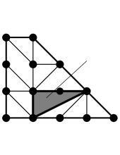
Figure 2. The dual subdivision of the curve of Figure 3.3. The triangle $\Delta_{v}$ is dual to the vertex $v$.

In [20], Mikhalkin assigns to a $3$-valent vertex $v$ of a simple tropical curve $(C,h)$ the (Mikhalkin) vertex multiplicity

(3.1) $$\operatorname{mult}_{\mathbb{C}}(v)=\operatorname{Area}(\Delta_{v}).$$

To the tropical curve $(C,h)$, he assigns the (Mikhalkin) multiplicity

(3.2) $$\operatorname{mult}_{\mathbb{C}}(C,h)=\prod_{v}\operatorname{mult}_{\mathbb{C}}(v)=\prod_{v}\operatorname{Area}(\Delta_{v}),$$

the product running over the $3$-valent vertices $v$ of $(C,h)$ and $\Delta_{v}$ is the triangle in the subdivision $\Delta_{C}$ dual to $v$ (cf., Definition 3.4 and Figure 2). If $v$ has adjacent edges $e_{1}$,$e_{2}$, and $e_{3}$, then the vertex multiplicity $\operatorname{mult}_{\mathbb{C}}(v)$ equals the Euclidian area of the parallelogram spanned by any two of the direction vectors starting at $v$.

Example 3.3 (cont’d). The dual subdivision of the tropical curve of Example 3.3 consists of $2$ triangles of (normalized) area $2$ and $9$ triangles of area $1$. The Mikhalkin multiplicity is thus $\operatorname{mult}_{\mathbb{C}}(C)=2^{2}\cdot 1^{9}=4$. (The quadrangle does not contribute to $\operatorname{mult}_{\mathbb{C}}(C)$.)

We associate to a tropical curve $(C,h)$ a refined weight. Recall that, for an integer $n$, we denote by

$$[n]_{y}=\frac{y^{n/2}-y^{-n/2}}{y^{1/2}-y^{-1/2}}=y^{(n-1)/2}+\cdots+y^{-(n-1)/2}$$

the quantum number of $n$. In particular, $[n]_{1}=n$. We can think about $[n]_{y}$ as a (shifted) $q$-analog of $n$.

Definition 3.5.

The refined vertex multiplicity of a $3$-valent vertex $v$ of a simple tropical curve $(C,h)$ is

(3.3) $$\operatorname{mult}(v;y)=[\operatorname{Area}(\Delta_{v})]_{y}.$$

The refined multiplicity of a simple tropical curve $(C,h)$ is

(3.4) $$\operatorname{mult}(C,h;y)=\prod_{v}[\operatorname{Area}(\Delta_{v})]_{y},$$

the product running over the $3$-valent vertices of $(C,h)$.

Example 3.3 (cont’d). The refined multiplicity of vertex $v$ of the tropical curve of Example 3.3 is $[\operatorname{Area}(\Delta_{v})]_{y}=[2]_{y}=y^{1/2}+y^{-1/2}$. As the dual subdivision consists of $2$ triangles of area $2$ and $9$ triangles of area $1$, the refined multiplicity of $(C,h)$ is

$$\operatorname{mult}(C,h;y)=(y^{1/2}+y^{-1/2})^{2}\cdot 1^{9}=y+2+y^{-1}.$$

(Again, the quadrangle does not contribute.)

We now define the tropical refinement of Severi degrees. For smooth toric surfaces, these invariants conjecturally agree with the refined invariants $\widetilde{N}^{X(\Delta),L(\Delta),\delta}(y)$, provided $L(\Delta)$ is sufficiently ample, see Conjecture 2.12.

As with classical curve counting, we require the configuration of tropical points to be in tropically generic position; the precise definition is given in [20, Definition 4.7]. Roughly, tropically generic means there are no tropical curves of unexpectedly small degree passing through the points. By [20, Proposition 4.11], the set of such points configurations is open and dense in the space of point configurations in ${\mathbb{R}}^{2}$. An important example of a tropically generic point configuration is the following. The combinatorics of tropical curves passing through such configurations is essentially given by the floor diagrams of Section 5.

Definition 3.6 ([5]).

Let $\Delta$ be a lattice polygon. A point configuration $\Pi=\{(x_{1},y_{1}),\dots,(x_{N},y_{N})\}$ in ${\mathbb{R}}^{2}$ is called vertically stretched with respect to $\Delta$ if, for every tropical curve $C$ of degree $\Delta$, we have

(3.5) $$\begin{split}\min_{i\neq j}|y_{i}-y_{j}|>&\max_{i\neq j}|x_{i}-x_{j}|\cdot|\text{maximal slope of an edge of }C|\\ &\hskip 90.00014pt\cdot\text{(number of edges of $C$)}.\end{split}$$

The notion of a vertically stretched point configuration for a fixed polygon $\Delta$ is well-defined, as (3.5) depends only on $\Pi$ and the finitely many combinatorial types of tropical curves of degree $\Delta$. Our definition of a vertically stretched point configuration is slightly more restricted than in [7, Section 5] but has the advantage of being explicit. It is sufficient for the floor decomposition techniques of tropical curves [5].

Definition 3.7.

Fix a lattice polygon $\Delta$ and $\delta\geq 0$.

1. The (tropical) refined Severi degree $N^{\Delta,\delta}(y)$ of the pair $(X(\Delta),L(\Delta))$ is

   (3.6) $$N^{\Delta,\delta}(y):=\sum_{(C,h)}\operatorname{mult}(C,h;y),$$

   where the sum is over all $\delta$-nodal tropical curves $(C,h)$ of degree $\Delta$ passing through $|\Delta\cap{\mathbb{Z}}^{2}|-1-\delta$ tropically generic points.

2. The (tropical) irreducible refined Severi degree of $(X(\Delta),L(\Delta))$ is

   (3.7) $$N_{0}^{\Delta,\delta}(y):=\sum_{(C,h)}\operatorname{mult}(C,h;y),$$

   the sum ranging over all irreducible tropical curves of degree $\Delta$ with $\delta$ nodes passing through $|\Delta\cap{\mathbb{Z}}^{2}|-1-\delta$ tropically generic points.

By Theorem 4.13, the tropical irreducible refined Severi degree agrees with its non-tropical version defined in (2.10) for ${\mathbb{P}}^{2}$, Hirzebruch surfaces and rational ruled surfaces. Note that a tropical curve through generic points is, by definition, necessarily simple. Itenberg and Mikhalkin showed that both refined tropical enumerations give indeed invariants.

Theorem 3.8 ([17, Theorem 1]).

The sum (3.7), and thus $N_{0}^{\Delta,\delta}(y)$, are independent of the tropical point configuration, as long as the configuration is generic.

Corollary 3.9.

The sum in (3.6), and thus $N^{\Delta,\delta}(y)$, are independent of the tropical point configuration, as long as the configuration is generic.

Proof.

The refined Severi degree can be expressed in terms of the irreducible refined Severi degrees, which are, by Theorem 3.8, independent of the specific location of the points.

Specifically, let $\Pi\subset{\mathbb{R}}^{2}$ be a tropically generic set of $|\Delta\cap{\mathbb{Z}}^{2}|-1-\delta$ points. Then (see also [1, Section 2.3])

(3.8) $$N^{\Delta,\delta}(y)=\sum_{\Pi=\cup\Pi_{i}}\sum_{(\Delta_{i},\delta_{i})}\prod_{i}N^{\Delta_{i},\delta_{i}}_{0}(y),$$

where the first sum is over all partitions of $\Pi$, and the second sum is over all pairs $(\Delta_{i},\delta_{i})$ which satisfy

(3.9) $$\begin{split}|\Pi_{i}|=&|\Delta_{i}\cap{\mathbb{Z}}^{2}|-1-\delta_{i},\quad\text{for all }1\leq i\leq t,\\ \Delta=&\Delta_{1}+\cdots+\Delta_{t}\quad\text{(Minkowski sum)},\\ \delta=&\sum_{i=1}^{t}\delta_{i}+\sum_{1\leq i<j\leq t}{\mathcal{M}}(\Delta_{i},\Delta_{j}).\end{split}$$

Here, again ${\mathcal{M}}(\Delta_{i},\Delta_{j})=\tfrac{1}{2}(\operatorname{Area}(\Delta_{i}+\Delta_{j})-\operatorname{Area}(\Delta_{i})-\operatorname{Area}(\Delta_{j}))$ is the mixed area of the polygons $\Delta_{i}$ and $\Delta_{j}$. ∎

At $y=1$, we recover Mikhalkin’s (Complex) Correspondence Theorem.

Theorem 3.10 (Mikhalkin’s (Complex) Correspondence Theorem [20, Theorem 1]).

For any lattice polygon $\Delta$:

1. the (tropical) Severi degree $N^{\Delta,\delta}(1)$ equals the (classical) Severi degree $N^{\Delta,\delta}$, and

2. the (tropical) irreducible Severi degree $N_{0}^{\Delta,\delta}(1)$ equals the irreducible (classical) Severi degree $N_{0}^{\Delta,\delta}$.

At $y=-1$, we recover Mikhalkin’s Real Correspondence Theorem. The classical Welschinger invariant $W^{\Delta,\delta}(\Pi)$ and the irreducible classical Welschinger invariant $W_{0}^{\Delta,\delta}(\Pi)$ count real curves resp. irreducible real curves of degree $\Delta$ with $\delta$ nodes through the real point configuration $\Pi$, counted with Welschinger sign. In positive genus, unlike for Severi degrees, both invariants depend on the point configuration $\Pi$, even for generic $\Pi$. For details see [20, Section 7.3].

Theorem 3.11 (Mikhalkin’s Real Correspondence Theorem [20, Theorem 6]).

For any lattice polygon $\Delta$:

1. the (tropical) Welschinger invariant $W_{{\mathrm{trop}}}^{\Delta,\delta}$ equals the (classical) Welschinger invariant $W^{\Delta,\delta}(\Pi)$ for some real point configuration $\Pi$, and

2. the irreducible (tropical) Welschinger invariant $W_{0,{\mathrm{trop}}}^{\Delta,\delta}$ equals the irreducible (classical) Welschinger invariant $W_{0}^{\Delta,\delta}(\Pi)$ for some real point configuration $\Pi$.

Remark 3.12.

The refined Severi degrees $N^{\Delta,\delta}(y)$ thus interpolate between Severi degrees and Welschinger invariants. Similarly, the refined irreducible Severi degrees $N_{0}^{\Delta,\delta}(y)$ interpolate between irreducible (classical) Severi degrees and irreducible (classical) Welschinger invariants.

4. Properties of refined Severi degrees

In this section, we show a few properties of refined Severi degrees. Specifically, we discuss the polynomiality of refined Severi degrees in the parameters of $\Delta$ in Section 4.1, conjecture the polynomiality of their coefficients (as Laurent polynomials in $y$) in Section 4.2, discuss implications for the conjectures of Göttsche and Shende in Section 4.3, and irreducible refined Severi degrees in Section 4.4.

4.1. Refined node polynomials

We will now prove Conjecture 2.12 for the projective plane ${\mathbb{P}}^{2}$ and $\delta\leq 10$, for ${\mathbb{P}}^{1}\times{\mathbb{P}}^{1}$ for $\delta\leq 6$ and for all Hirzebruch surfaces $\operatorname{\Sigma}_{m}$ for $\delta\leq 2$ and ${\mathbb{P}}(1,1,m)$ for $\delta\leq 2$.

First we state the existence of refined node polynomials $N_{\delta}(d;y)$, $N_{\delta}(c,d,m;y)$, $N_{\delta}(d,m;y)$, refining some results of [10] and [1]. The proof of the following theorem is in Section 6.

Theorem 4.1.

For fixed $\delta\geq 1$:

1. (${\mathbb{P}}^{2}$) There is a polynomial $N_{\delta}(d;y)\in{\mathbb{Q}}[y^{\pm 1}][d]$ of degree $2\delta$ in $d$ such that, for $d\geq\delta$,

   $$N_{\delta}(d;y)=N^{d,\delta}(y).$$

2. (Hirzebruch surface) There is a polynomial $N_{\delta}(c,d,m;y)\in{\mathbb{Q}}[y^{\pm 1}][c,d,m]$ of degree $\delta$ in $c,m$ and $2\delta$ in $d$ such that, for $c+m\geq 2\delta$ and $d\geq\delta$

   $$N_{\delta}(c,d,m;y)=N^{(\operatorname{\Sigma}_{m},cF+dH),\delta}(y).$$

3. (${\mathbb{P}}(1,1,m)$) There is a polynomial $N_{\delta}(d,m;y)\in{\mathbb{Q}}[y^{\pm 1}][d,m]$ of degree $2\delta$ in $d$ and $\delta$ in $m$ such that, for $d\geq\delta$ and $m\geq 2\delta$,

   $$N_{\delta}(d,m;y)=N^{{\mathbb{P}}(1,1,m),dH),\delta}(y).$$

We call the polynomials $N_{\delta}(d;y)$, $N_{\delta}(c,d,m;y)$, and $N_{\delta}(d,m;y)$ refined node polynomials.

Remark 4.2.

Theorem 4.1 generalizes to toric surfaces from “$h$-transverse” polygons with bounds exactly as in Theorems 1.2 and 1.3 in [1]. The argument of [1] generalizes to the refined setting by replacing all (Mikhalkin) weights by refined weights. As the argument is long and technical, we do not reproduce it here and restrain ourselves to more manageable cases.

Theorem 4.3.

1. (${\mathbb{P}}^{2}$) For $\delta\leq 10$ and $d\geq\delta/2+1$ we have

   $${\widetilde{N}}^{d,\delta}(y)=N_{\delta}(d)=N^{d,\delta}(y).$$

2. For $\delta\leq 6$ and $c,d\geq\delta/2$, we have

   $${\widetilde{N}}^{({\mathbb{P}}^{1}\times{\mathbb{P}}^{1},cF+dH),\delta}(y)=N_{\delta}(c,d,0;y)=N^{({\mathbb{P}}_{1}\times{\mathbb{P}}_{1},cF+dH),\delta}(y).$$

3. (Hirzebruch surfaces) For $\delta\leq 2$ and $d\geq 1$, $c\geq\delta$ we have

   $${\widetilde{N}}^{(\operatorname{\Sigma}_{m},cF+dH),\delta}(y)=N_{\delta}(c,d,m;y)=N^{(\operatorname{\Sigma}_{m},cF+dH),\delta}(y).$$

4. (${\mathbb{P}}(1,1,m)$) For $\delta\leq 2$ and $d\geq 2$ and $m\geq 1$ we have

   $$N_{\delta}(d,m;y)=N^{({\mathbb{P}}(1,1,m),d),\delta}(y).$$

   and $N_{\delta}(d,m;y)$ is given by Conjecture 2.16 and Remark 2.17.

Proof.

In [14] we have computed $\widetilde{N}^{(S,L),\delta}(y)$ for all $(S,L)$ and all $\delta\leq 10$. It is a polynomial of degree $\delta$ in the intersection numbers $L^{2}$, $LK_{S}$, $K_{S}^{2}$ and $\chi({\mathcal{O}}_{S})$.

(1) In the case $(S,L)=({\mathbb{P}}^{2},{\mathcal{O}}(d))$ this gives that $\widetilde{N}^{d,\delta}(y)$ as a polynomial of degree $2\delta$ in $d$. Using the recursion 2.7 we compute $N^{d,\delta}(y)$ for all $\delta\leq 10$ and all $d\leq 30$. We find that $N^{d,\delta}(y)=\widetilde{N}^{d,\delta}(y)$ for $\delta\leq 10$, and $\frac{\delta}{2}+1\leq d\leq 30$. We also know by Theorem 4.1 that $N_{\delta}(d)$ is a polynomial of degree $2\delta$ in $d$, and that $N_{\delta}(d)=N^{d,\delta}(y)$ for $d\geq\delta$. Thus for $0\leq\delta\leq 10$ the two polynomials $N_{\delta}(d)$ and $\widetilde{N}^{d,\delta}(y)$ of degree $2\delta$ in $d$ have the same value for $\delta\leq d\leq 30$. Thus they are equal.

(2) Is very similar to (1). We compute $N^{({\mathbb{P}}_{1}\times{\mathbb{P}}_{1},cF+dH),\delta}(y)$ for $c\leq 18$ and $d\leq 12$ and $\delta\leq 6$. We find that in this realm $N^{({\mathbb{P}}_{1}\times{\mathbb{P}}_{1},cF+dH),\delta}(y)={\widetilde{N}}^{({\mathbb{P}}^{1}\times{\mathbb{P}}^{1},cF+dH),\delta}(y)$ for $c,d\geq\delta/2$. We know by Theorem 4.1 and symmetry, that $N_{\delta}(c,d,0;y)$ is a polynomial of bidegree $(\delta,\delta)$ in $c,d$. Thus for $0\leq\delta\leq 6$, the two polynomials $N_{\delta}(c,d,0;y)$ and ${\widetilde{N}}^{({\mathbb{P}}^{1}\times{\mathbb{P}}^{1},cF+dH),\delta}(y)$ have the same value, whenever $18\geq c\geq 2\delta$, $12\geq d\geq\delta$. Thus they are equal.

(3) This case is again similar. We compute $N^{(\operatorname{\Sigma}_{m},cF+dH),\delta}(y)$ for $c\leq 6$ and $d\leq 6$, $m\leq 4$ and $\delta\leq 2$. The claim follows in the same way as before.

(4) We compute $N^{({\mathbb{P}}(1,1,m)dH),\delta}(y)$ for $d\leq 6$, $m\leq 6$ and $\delta\leq 2$. The claim follows in the same way as before. ∎

Corollary 4.4.

The coefficients of the refined invariants ${\widetilde{N}}^{(S,L),\delta}(y)$ are non-negative, i.e.,

$${\widetilde{N}}^{(S,L),\delta}(y)\in{\mathbb{Z}}_{\geq 0}[y^{\pm 1}]$$

provided either

• $S={\mathbb{P}}^{2}$, $L=dH$, $\delta\leq 10$, and $d\geq\tfrac{d}{2}+1$, or

• $S={\mathbb{P}}^{1}\times{\mathbb{P}}^{1}$, $L=cF+dH$, $\delta\leq 6$, and $c,d\geq\delta/2$.

• $S=\operatorname{\Sigma}_{m}$, $L=cF+dH$, $\delta\leq 2$, and $d\geq 1$, $c\geq\delta$.

• $S={\mathbb{P}}(1,1,m)$, $L=dH$, $\delta\leq 2$, and $d\geq 2$, $m\geq 1$.

Proof.

For any lattice polygon, the refined Severi degree $N^{\Delta,\delta}(y)$ is a Laurent polynomial in $y$ with non-negative coefficients. The corollary follows from Theorem 4.3. ∎

Conjecture 4.5.

For any smooth projective surface $S$ and $\delta$-very ample line bundle $L$ on $S$, the refined invariants ${\widetilde{N}}^{(S,L),\delta}(y)$ have non-negative coefficients.

We have the following evidence for this conjecture: In [15] Conjecture 2.7 is proven for $S$ an abelian or K3 surface, and the positivity of ${\widetilde{N}}^{(S,L),\delta}(y)$ follows for all line bundles $L$ on $S$. If $S$ is a toric surface and $L$ is $\delta$-very ample on $S$, then Conjecture 4.5 is implied by Conjecture 2.12. Numerical computations give in all examples considered that Conjecture 4.5 is true. Comparing with (2.6) numerical checks confirm that, in the realm checked, for $l>\delta$ all the coefficients of $(\frac{t}{g(y,t)})^{l}$ of degree at most $\delta$ in $t$ are positive. If $L$ is $\delta$-very ample we expect $\chi(L)>\delta$ and also $\chi(L)$ that is large with respect to $K_{S}^{2}$ and $LK_{S}$. Therefore we would expect that all coefficients of the left hand side of (2.6) of degree at most $\delta$ in $t$ are nonnegative.

4.2. Coefficient polynomiality of refined Severi degrees

The refined Severi degrees $N^{d,\delta}(y)$ of ${\mathbb{P}}^{2}$, as Laurent polynomial in $y$, have non-negative integral coefficients. Furthermore, for fixed $\delta$, these coefficients behave polynomially in $d$, for sufficiently large $d$, by Theorem 4.1. In this section, we conjecture that particular coefficients of the refined Severi degree are polynomial for $d$ independent of $\delta$ (Conjecture 4.8). We also give enumerative meaning to the first leading coefficient (Proposition 4.10). For simplicity, we consider only ${\mathbb{P}}^{2}$ in this section. Throughout this section, we fix the number of nodes $\delta\geq 1$.

Notation 4.6.

We denote the coefficients of the refined Severi degree by

$$N^{d,\delta}(y)=p^{\delta}_{d,0}\cdot y^{\delta}+p^{\delta}_{d,1}\cdot y^{\delta-1}+p^{\delta}_{d,2}\cdot y^{\delta-2}+\cdots+p^{\delta}_{d,\delta}\cdot y^{0}+\cdots+p^{\delta}_{d,0}\cdot y^{-\delta}$$

for $p^{\delta}_{d,0},p^{\delta}_{d,1},\dots,p^{\delta}_{d,\delta}\in{\mathbb{Z}}_{\geq 0}$.

Similarly, we write the coefficients of the refined node polynomial as

$$N_{\delta}(d;y)=p^{\delta}_{0}(d)\cdot y^{\delta}+p^{\delta}_{1}(d)\cdot y^{\delta-1}+p^{\delta}_{2}(d)\cdot y^{\delta-2}+\cdots+p^{\delta}_{\delta}(d)\cdot y^{0}+\cdots+p^{\delta}_{0}(d)\cdot y^{-\delta}$$

for polynomials $p^{\delta}_{0}(d),p^{\delta}_{1}(d),\dots,p^{\delta}_{\delta}(d)\in{\mathbb{Z}}[d]$.

From Theorem 4.1, the following is immediate.

Corollary 4.7.

For $0\leq i\leq\delta$, we have $p^{\delta}_{i}(d)=p^{\delta}_{d,i}$, whenever $d\geq\delta$.

Conjecturally, we have the lower bound $d\geq\tfrac{\delta}{2}+1$ (cf., Conjecture 2.11), which still depends on $\delta$. We conjecture that for the leading coefficients of the refined Severi degree, this dependence disappears.

Conjecture 4.8.

For $0\leq i\leq\delta$, we have $p^{\delta}_{i}(d)=p^{\delta}_{d,i}$, whenever $d\geq i+2$.

In other words, the larger the order of the coefficients of the refined Severi degree, the sooner the polynomiality kicks in. This conjecture was predicted as part of [14, Conj. 89], where in addition a formula for the coefficients $p^{\delta}_{i}(d)$ was conjectured. Proposition 4.10 below gives a new proof for $i=0$.

Remark 4.9.

1. Corollary 4.8 is part of [14, Conj. 89(1)].

2. More precisely this conjecture says that $p_{i}^{\delta}(d)$ is a polynomial of degree $2\delta$ in $d$, which is divisible by $\binom{\binom{d-1}{2}-3i}{\delta-i}$. Moreover [14, Conj. 86, Conj. 87] give a conjectural formula for the quotient $p_{i}^{\delta}(d)/\binom{\binom{d-1}{2}-3i}{\delta-i}$ in terms of the $\widetilde{N}^{d,\delta}(y)$ with $\delta\leq 3i$. Thus, assuming these conjectures, Theorem 4.3 gives a formula for $p^{\delta}_{i}(d)$ for $i\leq 3$.

3. Computational evidence suggests that for $d\geq 2$ the bound in Corollary 4.8 is optimal: $p_{i}^{\delta}(d)=p_{d,i}^{\delta}$, if and only if $d\geq i+2$. We checked this for $d\leq 14$, $\delta\leq 11$.

We give a formula for leading coefficient of the refined Severi degree. This result was also obtained in [14, Proposition 83] and [17, Proposition 2.11].

Proposition 4.10.

The leading coefficients of $N^{d,\delta}(y)$ is given by

$$p^{\delta}_{d,0}=\binom{\binom{d-1}{2}}{\delta}\quad\text{ for }d\geq 1.$$

The formula could be interpreted as the number of ways to choose $\delta$ of the $\binom{d-1}{2}$ nodes of a genus $0$ nodal curve $C$ of degree $d$, i.e. as the number of $\delta$-nodal curves obtained as partial resolutions of $C$.

We prove this proposition in Section 6.

The same formulas hold for the coefficients of the irreducible refined Severi degrees $N^{d,\delta}_{0}(y)$. Again we can write $N^{d,\delta}_{0}(y)=p_{d,0}^{\delta,0}y^{\delta}+p_{d,1}^{\delta,0}y^{\delta-1}+\ldots+p_{d,1}^{\delta,0}y^{-\delta+1}+p_{d,0}^{\delta,0}y^{-\delta}$. Assuming Conjecture 4.8, a similar result also holds for the $p_{d,i}^{\delta,0}$, because of the following lemma.

Lemma 4.11.

Assuming Conjecture 4.8, we have $p^{\delta,0}_{d,i}=p^{\delta}_{d,i}$ if $d\geq i+2$.

Proof.

If we specialize the formula (3.8) to $N^{d,\delta}(y)$, we express $N^{d,\delta}(y)-N^{d,\delta}_{0}(y)$ as a sum of products $\prod_{i=1}^{t}N^{d_{i},\delta_{i}}_{0}(y)$, with $t\geq 2$, $d=d_{1}+\ldots+d_{t}$ and

$$\delta=\sum_{i=1}^{t}\delta_{i}+\frac{1}{2}\sum_{1\leq i<j\leq t}\big{(}(d_{i}+d_{j})^{2}-d_{i}^{2}-d_{j}^{2}\big{)}.$$

It is an easy exercise to see that for given $d$ the rightmost sum is minimal if $t=2$ and $\{d_{1},d_{2}\}=\{1,d-1\}$, and the corresponding sum is $d-1$. Thus in all summands for $N^{d,\delta}(y)-N^{d,\delta}_{0}(y)$ we have $\delta-\sum_{i}\delta_{i}\geq d-1$. As the $N^{d_{i},\delta_{i}}_{0}(y)$ have degree at most $\delta_{i}$ in $y,y^{-1}$, we see that $p^{\delta}_{d,i}=p^{\delta,0}_{d,i}$ for $i<d-1$. ∎

The argument also shows that $N^{d,\delta}(y)=N^{d,\delta}_{0}(y)$ if $\delta\leq d-2$. Thus we obtain the following corollary

Corollary 4.12.

$N^{d,\delta}_{0}(y)=N_{\delta}(d;y)$ for $\delta\leq d-2$.

4.3. Numerical evidence for Göttsche and Shende’s conjectures

Theorem 4.1 and Theorem 4.3 provide strong evidence for Conjecture 2.7, Conjecture 2.11: On ${\mathbb{P}}^{2}$ and rational ruled surfaces, for $L$ sufficiently ample with respect to $\delta$, $N^{(S,L),\delta}(y)$ is indeed given by a node polynomial in $L^{2}$, $LK_{S}$, $K_{S}^{2}$ and $\chi({\mathcal{O}}_{S})$. Furthermore, if $\delta$ is not too large, we show that this polynomial coincides with ${\widetilde{N}}^{(S,L),\delta}(y)$. Unfortunately in the case of rational ruled surfaces we only prove this for $\delta\leq 2$. There is however more and stronger numerical evidence, even if it does not lead to a proof of formulas for higher $\delta$. Below we list briefly some of this evidence.

1. In [14] the $N^{d,\delta}(y)$ have been computed for $d\leq 17$ and $\delta\leq 32$. Assuming Conjecture 2.7,Conjecture 2.11 this determines the power series $B_{1}(y,q)$ and $B_{2}(y,q)$ modulo $q^{29}$, and thus all the refined invariants ${\widetilde{N}}^{(S,L),\delta}(y)$ as polynomials in $L^{2}$, $LK_{S}$, $K_{S}^{2}$, $\chi({\mathcal{O}}_{S})$ for all $S$, $L$ and all $\delta\leq 28$. Denote for the moment $\widehat{N}^{(S,L),\delta}(y)$ the refined invariants obtained this way (and $\widehat{N}^{d,\delta}(y)$ the corresponding invariants of ${\mathbb{P}}^{2}$. For $\delta\leq 10$ (where the ${\widetilde{N}}^{(S,L),\delta}(y)$ have been computed in [14]) $\widehat{N}^{(S,L),\delta}(y)={\widetilde{N}}^{(S,L),\delta}(y)$.

   The computation mentioned above gives $N^{d,\delta}(y)=\widehat{N}^{d,\delta}(y)$ for $d\leq 17$ and $\delta\leq min(2d-2,28)$.

2. We have also computed the $N^{d,\delta}(y)$ for $d\leq 20$, $\delta\leq 20$, again within this realm $N^{d,\delta}(y)=\widehat{N}^{d,\delta}(y)$ for $\delta\leq 2d-2$.

3. We computed $N^{{\mathbb{P}}^{1}\times{\mathbb{P}}^{1},cF+dH),\delta}$ for arbitrary $\delta$ and $c,d\leq 8$. We find in this realm $N^{({\mathbb{P}}^{1}\times{\mathbb{P}}^{1},cF+dH),\delta}=\widetilde{N}^{({\mathbb{P}}^{1}\times{\mathbb{P}}^{1},cF+dH),\delta}$ for $\delta\leq min(2c,2d)$.

4. We computed $N^{(\Sigma_{m},cF+dH),\delta}(y)$ for $m\leq 10$, $\delta\leq 10$, $d\leq 6$, $c\leq 10$. We find in this realm $N^{(\Sigma_{m},cF+dH,\delta}(y)={\widetilde{N}}^{(\Sigma_{m},cF+dH,\delta}(y)$ if $\delta\leq min(2d,c)$.

4.4. On the relation with irreducible refined Severi degrees

We show that the irreducible refined Severi degree, formally defined in (2.10) for ${\mathbb{P}}^{2}$, Hirzebruch surfaces and rational ruled surfaces, agrees with the refined enumeration of irreducible tropical curves. It therefore follows that also the irreducible refined Severi degree has non-negative coefficients.

Theorem 4.13.

The tropical irreducible refined Severi degree $N_{0}^{\Delta,\delta}(y)$ agrees with the irreducible refined Severi degree defined in (2.10).

The refined multiplicity of an irreducible tropical curve by definition has non-negative integer coefficients in $y^{\pm 1}$. Therefore, we have shown the following.

Corollary 4.14.

$N_{0}^{\Delta,\delta}(y)$ has non-negative integer coefficients.

Proof of Theorem 4.13..

Recall the relation (3.8)) between refined Severi degrees and their tropical irreducible analog

(4.1) $$N^{\Delta,\delta}(y)=\sum_{\Pi=\cup\Pi_{i}}\sum_{(\Delta_{i},\delta_{i})}\prod_{i}N^{\Delta_{i},\delta_{i}}_{0}(y),$$

where the first sum is over all partitions of $\Pi$, and the second sum is over all pairs $(\Delta_{i},\delta_{i})$ which satisfy (cf. (3.9))

(4.2) $$\begin{split}|\Pi_{i}|=&|\Delta_{i}\cap{\mathbb{Z}}^{2}|-1-\delta_{i},\quad\text{for all }1\leq i\leq t,\\ \Delta=&\Delta_{1}+\cdots+\Delta_{t}\quad\text{(Minkowski sum)},\\ \delta=&\sum_{i=1}^{t}\delta_{i}+\sum_{1\leq i<j\leq t}{\mathcal{M}}(\Delta_{i},\Delta_{j}).\end{split}$$

Here, again ${\mathcal{M}}(\Delta_{i},\Delta_{j})=\tfrac{1}{2}(\operatorname{Area}(\Delta_{i}+\Delta_{j})-\operatorname{Area}(\Delta_{i})-\operatorname{Area}(\Delta_{j}))$ is the mixed area of the polygons $\Delta_{i}$ and $\Delta_{j}$.

Any collection of lattice polygons $\Delta_{1},\Delta_{2},\dots,\Delta_{t},\Delta$ and non-negative integers $\delta_{1},\dots,\delta_{t},\delta$ satisfying the second and third condition of (4.2) also satisfy

$$\sum_{i=1}^{t}(\dim\Delta_{i}-\delta_{i})=\dim\Delta-\delta,$$

where we write $\dim\Delta=|\Delta\cap{\mathbb{Z}}^{2}|-1$. Indeed, both sides equal the number of point conditions of a tropical curve of degree $\Delta$ with $\delta$ nodes which has irreducible components of degrees $\Delta_{i}$ with $\delta_{i}$ nodes, respectively. Furthermore, we have $\operatorname{mult}(C;y)=\prod_{i=1}^{t}\operatorname{mult}(C_{i};y)$.

The exponential generating functions of the refined Severi degrees $N^{\Delta,\delta}(y)$ and the tropical irreducible refined Severi degree $N_{0,{\mathrm{trop}}}^{\Delta,\delta}(y)$ thus satisfy

(4.3) $$\exp\left(\sum_{\Delta,\delta}\frac{z^{\dim\Delta-\delta}}{(\dim\Delta-\delta)!}v^{\Delta}N_{0,{\mathrm{trop}}}^{\Delta,\delta}(y)\right)=1+\sum_{\Delta,\delta}\frac{z^{\dim\Delta-\delta}}{(\dim\Delta-\delta)!}v^{\Delta}N^{\Delta,\delta}(y),$$

where we define $v^{\Delta}\cdot v^{\Delta^{\prime}}:=v^{\Delta+\Delta^{\prime}}$ for lattice polygons $\Delta$ and $\Delta^{\prime}$ and both sums are over all lattice polygons $\Delta$ (up to translation) and $\delta\geq 0$. Comparing (4.3) and (2.10), the result follows. ∎

5. $y$-Weighted Floor Diagrams and Templates

Floor diagrams are purely combinatorial representations of tropical curves. They exist for all “$h$-transverse” polygons $\Delta$. We focus mostly on the cases $S={\mathbb{P}}^{2}$, $\Sigma_{m}$, and ${\mathbb{P}}(1,1,m)$, all whose moment polygons are $h$-transverse. More specifically, if we consider tropical curves through a vertically stretched point configuration (see Definition 3.6) the tropical curves are uniquely encoded by a “marking” of a floor diagram and, vice versa, every marked floor diagram corresponds to a tropical curve. This gives a purely combinatorial way to compute refined Severi degrees for toric surfaces with $h$-transverse polygons. Floor diagrams were invented (in the unrefined setting) by Brugallé and Mikhalkin [6, 7].

5.1. Floor Diagrams

We now briefly review the marked floor diagrams of Brugallé and Mikhalkin [6, 7] for surfaces $S={\mathbb{P}}^{2}$, $S={\mathbb{P}}(1,1,m)$, and $S=\operatorname{\Sigma}_{m}$, with some emphasis on the ${\mathbb{P}}^{2}$ case. We present them in the notation of Ardila and Block [1], following Fomin and Mikhalkin [10]. In each case, we fix a polygon $\Delta$ (cf. Figure 3):

• (${\mathbb{P}}^{2}$ case) $\Delta=\operatorname{conv}((0,0),(0,d),(d,0))$, for $d\geq 1$, or

• ($\operatorname{\Sigma}_{m}$ case) $\Delta=\operatorname{conv}((0,0),(0,d),(c,d),(c+md,0))$, for $c,d,m\geq 1$, or

• (${\mathbb{P}}(1,1,m)$ case) $\Delta=\operatorname{conv}((0,0),(0,d),(dm,0))$, for $d,m\geq 1$. In this case, set $c=0$.

Figure 3. Lattice polygons of the Hirzebruch surface $\Sigma_{m}$ with line bundle $L=dH+cF$ (left) and ${\mathbb{P}}(1,1,m)$ with $L=dH$ (right). In both cases $m=2$. For $S={\mathbb{P}}^{2}$, we set $c=0$ and $m=1$.

Definition 5.1.

A $\Delta$-floor diagram ${\mathcal{D}}$ consists of:

1. A graph on a vertex set $\{1,\dots,d\}$, possibly with multiple edges, with edges directed $i\to j$ if $i<j$.

2. A sequence $(s_{1},\dots,s_{d})$ of non-negative integers such that $s_{1}+\cdots+s_{d}=c$. (If $S={\mathbb{P}}(1,1,m)$ then all $s_{i}$ equal $0$.)

3. (Divergence Condition) For each vertex $j$ of ${\mathcal{D}}$, we have

   $$\text{div}(j)\stackrel{{\scriptstyle\text{def}}}{{=}}\sum_{\tiny\begin{array}[]{c}\text{edges }e\\ j\stackrel{{\scriptstyle e}}{{\to}}k\end{array}}{\mathrm{wt}}(e)-\sum_{\tiny\begin{array}[]{c}\text{edges }e\\ i\stackrel{{\scriptstyle e}}{{\to}}j\end{array}}{\mathrm{wt}}(e)\leq m+s_{j}.$$

The last condition says that at every vertex of ${\mathcal{D}}$ the total weight of the outgoing edges is larger by at most $m+s_{j}$ than the total weight of the incoming edges.

We loosely think of $\Delta$ as the degree of the floor diagram ${\mathcal{D}}$. If $S={\mathbb{P}}^{2}$, we say that ${\mathcal{D}}$ is of degree $d$. A floor diagram is connected if its underlying graph is. If ${\mathcal{D}}$ is connected its genus is the genus of the underlying graph. A connected floor diagram ${\mathcal{D}}$ of degree $\Delta$ and genus $g$ has cogenus $\delta({\mathcal{D}})$ equal to the number of interior lattice points in $\Delta$ minus $g$.

If ${\mathcal{D}}$ is not connected, there are lattice polygons $\Delta_{1},\Delta_{2},\dots$ such that their Minkowski sum equals $\Delta_{1}+\Delta_{2}+\cdots=\Delta$ and the $\Delta_{i}$ are the degrees of the connected components of ${\mathcal{D}}$. Let $\delta_{1},\delta_{2},\dots$ be the cogenera of the connected components. Similarly to the case of tropical curves, we define the cogenus

$$\delta({\mathcal{D}})=\sum_{i}\delta_{i}+\sum_{i<j}{\mathcal{M}}(\Delta_{i},\Delta_{j}),$$

where again ${\mathcal{M}}(\Delta_{i},\Delta_{j}):=\tfrac{1}{2}(\operatorname{Area}(\Delta_{i}+\Delta_{j})-\operatorname{Area}(\Delta_{i})-\operatorname{Area}(\Delta_{j}))$ is the mixed area of $\Delta_{i}$ and $\Delta_{j}$. As before, $\operatorname{Area}(-)$ is the normalized area, given by twice the Euclidian area in ${\mathbb{R}}^{2}$.

The refined multiplicity of tropical curves (see Definition 3.5) translates to floor diagram as follows, yielding a purely combinatorial formula for the refined Severi degrees for $\operatorname{\Sigma}_{m}$ and ${\mathbb{P}}(1,1,m)$ in Definition 5.6.

Definition 5.2.

We define the refined multiplicity $\operatorname{mult}({\mathcal{D}},y)$ of a floor diagram ${\mathcal{D}}$ as

$$\operatorname{mult}({\mathcal{D}},y)=\prod_{\text{edges }e}\left([{\mathrm{wt}}(e)]_{y}\right)^{2}.$$

Notice that the weight $\operatorname{mult}({\mathcal{D}},y)$ is a Laurent polynomial in $y$ with positive integral coefficients. We draw floor diagrams using the convention that vertices in increasing order are arranged left to right. Edge weights of $1$ are omitted.

Example 5.3.

An example of a floor diagram for ${\mathbb{P}}^{2}$ of degree $d=4$, genus $g=1$, cogenus $\delta=2$, divergences $1,1,0,-2$, and multiplicity $\operatorname{mult}({\mathcal{D}};y)=(y^{-1/2}+y^{1/2})^{2}=y^{-1}+2+y$ is drawn below.

To a floor diagram we associate a last statistic, as in [10, Section 1]. Notice that this statistic is independent of $y$.

Definition 5.4.

A marking of a floor diagram ${\mathcal{D}}$ is defined by the following four step process

Step 1: For each vertex $j$ of ${\mathcal{D}}$ create $s_{j}$ new indistinguishable vertices and connect them to $j$ with new edges directed towards $j$.

Step 2: For each vertex $j$ of ${\mathcal{D}}$ create $m+s_{j}-div(j)$ new indistinguishable vertices and connect them to $j$ with new edges directed away from $j$. This makes the divergence of vertex $j$ equal to $m$.

Step 3: Subdivide each edge of the original floor diagram ${\mathcal{D}}$ into two directed edges by introducing a new vertex for each edge. The new edges inherit their weights and orientations. Denote the resulting graph $\widetilde{{\mathcal{D}}}$.

Figure 4. The result of applying Steps 1-3 to the floor diagram of Example 5.3

Step 4: Linearly order the vertices of $\widetilde{{\mathcal{D}}}$ extending the order of the vertices of the original floor diagram ${\mathcal{D}}$ such that, as before, each edge is directed from a smaller vertex to a larger vertex.

The extended graph $\widetilde{{\mathcal{D}}}$ together with the linear order on its vertices is called a marked floor diagram, or a marking of the original floor diagram ${\mathcal{D}}$.

Figure 5. A marking of the floor diagram of Figure 4

We want to count marked floor diagrams up to equivalence. Two markings $\widetilde{{\mathcal{D}}}_{1}$, $\widetilde{{\mathcal{D}}}_{2}$ of a floor diagram ${\mathcal{D}}$ are equivalent if there exists an automorphism of weighted graphs which preserves the vertices of ${\mathcal{D}}$ and maps $\widetilde{{\mathcal{D}}}_{1}$ to $\widetilde{{\mathcal{D}}}_{2}$. The number of markings $\nu({\mathcal{D}})$ is the number of marked floor diagrams $\widetilde{{\mathcal{D}}}$ up to equivalence.

Example 5.5.

The floor diagram ${\mathcal{D}}$ of Example 5.3 has $\nu({\mathcal{D}})=3+4=7$ markings (up to equivalence): In step 3 the extra $1$-valent vertex connected to the third white vertex from the left can be inserted in three ways between the third and fourth white vertex (up to equivalence) and in four ways right of the fourth white vertex (again up to equivalence).

With these two statistics, we define a purely combinatorial notion of refined Severi degrees for $S={\mathbb{P}}^{2}$, $S=\operatorname{\Sigma}_{m}$, and $S={\mathbb{P}}(1,1,m)$. The combinatorial invariants agree with the refined Severi degree $N^{\Delta,\delta}(y)$ of Section 3 (Theorem 5.7). They also agree conjecturally with the refined invariants of Göttsche and Shende if $S$ is smooth and the line bundle is sufficiently ample (cf. Conjecture 2.12 and Theorem 4.3).

See Remark 5.8 for a discussion how to generalize to a much larger family of toric surfaces corresponding to “$h$-transverse” $\Delta$. Denote by $\operatorname{{\bf FD}}(\Delta,\delta)$ the set of $\Delta$-floor diagrams ${\mathcal{D}}$ with cogenus $\delta$.

Definition 5.6.

Fix $\delta\geq 0$ and let $\Delta$ be as above. We define the combinatorial refined Severi degree $N_{\mathrm{comb}}^{\Delta,\delta}(y)$ to be the Laurent polynomial in $y$ given by

(5.1) $$N_{\mathrm{comb}}^{\Delta,\delta}(y)=\sum_{{\mathcal{D}}\in\operatorname{{\bf FD}}(\Delta,\delta)}\operatorname{mult}({\mathcal{D}};y)\cdot\nu({\mathcal{D}}).$$

Theorem 5.7.

For $\Delta$ as in Definition 5.6 and $\delta\geq 0$, the combinatorial refined Severi degree and the refined Severi degree agree:

$$N_{\mathrm{comb}}^{\Delta,\delta}(y)=N^{\Delta,\delta}(y).$$

Proof.

Let $\Pi\subset{\mathbb{R}}^{2}$ be a vertically stretched (Definition 3.6) configuration of $|\Delta\cap{\mathbb{Z}}^{2}|-1-\delta$ tropical points. In [7, Proposition 5.9], Brugallé and Mikhalkin construct an explicit bijection between the set of parametrized tropical curves of degree $\Delta$ with $\delta$ nodes passing through $\Pi$ and the set of marked $\Delta$-floor diagrams of cogenus $\delta$. This bijection is $y$-weight preserving. ∎

In the sequel, we will usually write $N$ instead of $N_{\mathrm{comb}}$ even while referring to the combinatorial defined refined Severi degree if no confusion can occur.

Remark 5.8.

We expect the results in this section to also hold for toric surfaces from “$h$-transverse” polygons $\Delta$: Brugallé and Mikhalkin [7] construct marked floor diagrams for this class of polygons. One can define a notion of combinatorial refined Severi degrees for any toric surface from an “$h$-transverse polygon”: simply replace the multiplicity of a “$\Delta$-floor diagram” ${\mathcal{D}}$ in [1, Equation (Severi1)] by the $y$-weight

$$\operatorname{mult}({\mathcal{D}},y)=\prod_{\text{edges }e}\left([{\mathrm{wt}}(e)]_{y}\right)^{2}.$$

Theorem 5.7 can then be extended to the more general setting. We omit the details here to avoid too many technicalities.

5.2. Templates

The following gadget was introduced by Fomin and Mikhalkin [10].

Definition 5.9.

A template $\Gamma$ is a directed graph (possibly with multiple edges) on vertices $\{0,\dots,l\}$, where $l\geq 1$, with edge weights ${\mathrm{wt}}(e)\in{\mathbb{Z}}_{>0}$, satisfying:

1. If $i\to j$ is an edge, then $i<j$.

2. Every edge $i\stackrel{{\scriptstyle e}}{{\to}}i+1$ has weight ${\mathrm{wt}}(e)\geq 2$. (No “short edges.”)

3. For each vertex $j$, $1\leq j\leq l-1$, there is an edge “covering” it, i.e., there exists an edge $i\to k$ with $i<j<k$.

Every template $\Gamma$ comes with some numerical data associated with it. Its length $\ell(\Gamma)$ is the number of vertices minus $1$. Its cogenus $\delta(\Gamma)$ is

(5.2) $$\delta(\Gamma)=\sum_{i\stackrel{{\scriptstyle e}}{{\to}}j}\bigg{[}(j-i){\mathrm{wt}}(e)-1\bigg{]}.$$

We define its $y$-multiplicity $\operatorname{mult}(\Gamma,y)$ to be

$$\operatorname{mult}(\Gamma,y)=\prod_{\text{edges }e}\left([{\mathrm{wt}}(e)]_{y}\right)^{2}.$$

See Figure 6 for examples.

For $1\leq j\leq\ell(\Gamma)$, let $\varkappa_{j}=\varkappa_{j}(\Gamma)$ denote the sum of the weights of edges $i\to k$ with $i<j\leq k$. So $\varkappa_{j}(\Gamma)$ equals the total weight of the edges of $\Gamma$ from a vertex left of $j$ to a vertex right of or equal to $j$. Define

$$k_{\min}(\Gamma)=\max_{1\leq j\leq l}(\varkappa_{j}-j+1).$$

This makes $k_{\min}(\Gamma)$ the smallest positive integer $k$ such that $\Gamma$ can appear in a floor diagram on $\{1,2,\dots\}$ with left-most vertex $k$. Lastly, set

$${\varepsilon}_{0}(\Gamma)=\left\{\begin{array}[]{ll}1&\text{if all edges starting at }0\text{ have weight }1,\\ 0&\text{otherwise,}\end{array}\right.$$

and

$${\varepsilon}_{1}(\Gamma)=\left\{\begin{array}[]{ll}1&\text{if all edges arriving at }l\text{ have weight }1,\\ 0&\text{otherwise,}\end{array}\right.$$

Figure 6 (taken from Fomin-Mikhalkin [10]) shows all templates $\Gamma$ with $\delta(\Gamma)\leq 2$.

Notice that, for each $\delta$, there are only a finite number of templates with cogenus $\delta$. At $y=1$, we recover Fomin and Mikhalkin’s template multiplicity $\prod_{e}{\mathrm{wt}}(e)^{2}$. It is clear that $\operatorname{mult}(\Gamma,y)$ is a Laurent polynomial with positive integral coefficients.

$\Gamma$	$\delta(\Gamma)$	$\ell(\Gamma)$	$\operatorname{mult}(\Gamma;y)$	${\varepsilon}_{0}(\Gamma)$	${\varepsilon}_{1}(\Gamma)$	$\varkappa(\Gamma)$	$k_{\min}(\Gamma)$
	1	1	$y^{-1}+2+y$	0	0	(2)	2
	1	2	1	1	1	(1,1)	1
	2	1	$y^{-2}+2y^{-1}+3+2y+y^{2}$	0	0	(3)	3
	2	1	$y^{-2}+4y^{-1}+6+4y+y^{2}$	0	0	(4)	4
	2	2	1	1	1	(2,2)	2
	2	2	$y^{-1}+2+y$	0	1	(3,1)	3
	2	2	$y^{-1}+2+y$	1	0	(1,3)	2
	2	3	1	1	1	(1,1,1)	1
	2	3	1	1	1	(1,2,1)	1

Figure 6. The templates with $\delta(\Gamma)\leq 2$.

5.3. Decomposition into Templates

A labeled floor diagram ${\mathcal{D}}$ with $d$ vertices decomposes into an ordered collection $(\Gamma_{1},\dots,\Gamma_{s})$ of templates as follows. If $S={\mathbb{P}}^{2}$ or ${\mathbb{P}}(1,1,m)$, then we set as before $c=0$. We treat $S={\mathbb{P}}^{2}$ as the special case of ${\mathbb{P}}(1,1,m)$ for $m=1$.

First, add an additional vertex $0$ ($<1$) to ${\mathcal{D}}$ and connect it to every vertex $j$ of ${\mathcal{D}}$ by $s_{j}$ many new edges of weight $1$ from $0$ to $j$ for each $1\leq j\leq d$. (For $S={\mathbb{P}}^{2}$ and $S={\mathbb{P}}(1,1,m)$, there is nothing to do, as $s_{j}=0$ for all $j$.) Second, add an additional vertex $d+1$ ($>d$), together with $m+s_{j}-\operatorname{div}(j)$ new edges of weight $1$ from $j$, for each $1\leq j\leq d$. The divergence sequence of the resulting diagram ${\mathcal{D}}^{\prime}$ is ${\bf a}:=(c,m,\dots,m)\in{\mathbb{Z}}_{\geq 0}^{d+1}$, after we remove the (superfluous) last entry. Now remove all short edges from ${\mathcal{D}}^{\prime}$, that is, all edges of weight $1$ between consecutive vertices. The result is an ordered collection of templates $(\Gamma_{1},\dots,\Gamma_{s})$, listed left to right. We also keep track of the initial vertices $k_{1},\dots,k_{s}$ of these templates.

Conversely, given the collection of templates ${\bf\Gamma}=(\Gamma_{1},\dots,\Gamma_{s})$, the initial vertices $k_{1},\dots,k_{s}$, and the divergence sequence $(c,m,\dots,m)\in{\mathbb{Z}}_{\geq 0}^{d+1}$, this process is easily reversed. To recover ${\mathcal{D}}^{\prime}$, we first place the templates at their starting points $k_{i}$ in the interval $[0,\dots,M]$, and add in all short edges we removed from ${\mathcal{D}}^{\prime}$. More precisely, we need to add $(a_{0}+\cdots+a_{j-1}-\varkappa_{k_{j}-j}(\Gamma_{i}))$ short edges between $j-1$ and $j$, where $\Gamma_{i}$ is the template containing $j$. The sequence $s$ records the number $s_{j}$ of edges between vertices $0$ and $j$. Finally, we remove the first and last vertices and their incident edges to obtain ${\mathcal{D}}$.

Example 5.10.

An example for $S={\mathbb{P}}^{2}$ of the decomposition of a labeled floor diagram into templates is illustrated below. Here, $k_{1}=2$ and $k_{2}=4$ and all $s_{j}=0$.

We record, for each ordered template collection ${\bf\Gamma}=(\Gamma_{1},\dots,\Gamma_{s})$, all valid “positions” $k_{i}$ that can occur in the template decomposition of a $\Delta$-floor diagram by the lattice points in a polytope. There are two cases. If $S={\mathbb{P}}^{2}$, we set

(5.3) $$\begin{split}A_{{\bf\Gamma}}(d)=\{&{\bf k}\in{\mathbb{R}}^{s}\,:\,k_{i}\geq k_{\min}(\Gamma_{i}),\\ &k_{i}+\ell(\Gamma_{i})\leq k_{i+1}\,\,\,(1\leq i<s),\,k_{s}+\ell(\Gamma_{s})\leq d+{\varepsilon}_{1}(\Gamma_{s})\}.\end{split}$$

If $S={\mathbb{P}}(1,1,m)$ or $S=\operatorname{\Sigma}_{m}$, we set

(5.4) $$\begin{split}A_{{\bf\Gamma}}(d)=\{&{\bf k}\in{\mathbb{R}}^{s}\,:\,k_{1}\geq 1-{\varepsilon}_{0}(\Gamma_{1}),\\ &k_{i}+\ell(\Gamma_{i})\leq k_{i+1}\,\,\,(1\leq i<s),\,k_{s}+\ell(\Gamma_{s})\leq d+{\varepsilon}_{1}(\Gamma_{s})\}.\end{split}$$

The first inequality in (5.3) says that, due to the divergence condition, templates cannot appear too early in a floor diagram. The first inequality in (5.4) says that the first starting position can be $0$ precisely when all outgoing edges of the first vertex of $\Gamma_{1}$ have weight $1$. The second resp. third inequality in (5.3) and (5.4) say that templates cannot overlap resp. cannot hang over at the end of the floor diagram.

We note that the lattice points in $A_{{\bf\Gamma}}(d)$ in (5.4) record all template positions if the divergence at the first vertex is at least $2\delta$: the quantity $\varkappa_{j}(\Gamma)$ is maximal, for a given $\delta(\Gamma)=\delta$, when $\Gamma$ is the template with two vertices and $\delta$ edges between them, each with weight $2$, and $j=1$. The condition $\text{div}(1)\geq 2\delta$ implies then that every collection of lattice points in the polytope can be the sequence of positions of templates, and vice versa. We always make the assumption $\text{div}(1)\geq 2\delta$ in Section 6, where we prove polynomiality of the refined Severi degrees for parameters in this regime (cf. Theorem 4.1).

5.4. Multiplicity, Cogenus, and Markings.

The refined multiplicity, cogenus, and markings of a floor diagram behave well under template decomposition, as in the unrefined case. If a floor diagram ${\mathcal{D}}$ has template decomposition ${\bf\Gamma}$, then by definition

$$\operatorname{mult}({\mathcal{D}};y)=\prod_{i=1}^{s}\operatorname{mult}(\Gamma_{i};y).$$

Furthermore, the decomposition of Section 5.3 is cogenus preserving, i.e., $\delta({\mathcal{D}})=\sum_{i=1}^{s}\delta(\Gamma_{i})$ (see [1, Section 3.3.2]). The number of markings of floor diagrams is expressible in terms of the number of “markings of the templates”: In Step 4 in Definition 5.4, instead of linearly ordering $\tilde{{\mathcal{D}}}$, we can order each template individually. To make this precise, associate to each template $\Gamma$ a polynomial $P_{\Gamma}(c,m;k)$ in $k$ which depends also on the parameters $c$ and $m$ of the polygon $\Delta$ (cf. Figure 3). Specifically, let $\Gamma_{(c,m,k)}$ denote the graph obtained from $\Gamma$ by first adding

$$c+(k+j-1)m-\varkappa_{j}(\Gamma)$$

short edges, making the divergence of all vertices $m$, and then subdividing each of the resulting graphs by introducing a new vertex for each edge. Let $P_{\Gamma}(c,m;k)$ be the number of linear extensions, up to equivalence, of the vertex poset of the graph $\Gamma_{(c,m,k)}$ extending the vertex order of $\Gamma$. Then

$$\nu({\mathcal{D}})=\prod_{i=1}^{s}P_{\Gamma_{i}}(c,m;k_{i}).$$

We can summarize the previous discussion in the following proposition.

Proposition 5.11.

The combinatorial refined Severi degree for

1. $S={\mathbb{P}}^{2}$, any $\delta\geq 1$ and $d\geq 1$, or

2. $S=\operatorname{\Sigma}_{m}$ resp. $S={\mathbb{P}}(1,1,m)$, $\delta\geq 1$ and $m,c,d\geq 1$ with $c+m\geq 2\delta$

is given by

(5.5) $$N_{\mathrm{comb}}^{\Delta,\delta}(y)=\sum_{{\bf\Gamma}:\,\sum_{i}\delta(\Gamma_{i})=\delta}\left[\Big{(}\prod_{i=1}^{s}\operatorname{mult}(\Gamma_{i},y)\Big{)}\sum_{{\bf k}\in A_{{\bf\Gamma}}(d)\cap{\mathbb{Z}}^{s}}\Big{(}\prod_{i=1}^{s}\ P_{\Gamma_{i}}(c,m;k_{i})\Big{)}\right],$$

the first sum running over all templates collections ${\bf\Gamma}=(\Gamma_{1},\dots,\Gamma_{s})$ with $\sum_{i=1}^{s}\delta(\Gamma_{i})=\delta$.

If $S=\operatorname{\Sigma}_{m}$ one can relax condition $m\geq 2\delta$ to $m+c\geq 2\delta$.

For $y=1$ and $S={\mathbb{P}}^{2}$, expression (5.5) specializes to [10, (5.13)]. For $y=1$ and $S=\operatorname{\Sigma}_{m}$ resp. $S={\mathbb{P}}(1,1,m)$, expression (5.5) specializes to [1, Proposition 3.3].

6. Polynomiality Proofs

We now use floor diagrams and templates to prove Theorem 4.1 and Proposition 4.10. The argument for the former is based on the combinatorial formula (5.5). Our technique is a $q$-analog extension of Fomin and Mikhalkin’s method [10, Section 5] for the ${\mathbb{P}}^{2}$ and Ardila and Block’s [1] for $\operatorname{\Sigma}_{m}$ and ${\mathbb{P}}(1,1,m)$. The method provides an algorithm to compute refined node polynomials for any $\delta$; see Remark 6.1 for a list for $\delta\leq 2$ for ${\mathbb{P}}^{2}$.

Theorem 4.1.

For fixed $\delta\geq 1$:

1. (${\mathbb{P}}^{2}$) There is a polynomial $N_{\delta}(d;y)\in{\mathbb{Q}}[y^{\pm 1}][d]$ of degree $2\delta$ in $d$ such that, for $d\geq\delta$,

   $$N_{\delta}(d;y)=N^{d,\delta}(y).$$

2. (Hirzebruch surface) There is a polynomial $N_{\delta}(c,d,m;y)\in{\mathbb{Q}}[y^{\pm 1}][c,d,m]$ of degree $\delta$ in $c,m$ and $2\delta$ in $d$ such that, for $c+m\geq 2\delta$ and $d\geq\delta$

   $$N_{\delta}(c,d,m;y)=N^{(\operatorname{\Sigma}_{m},cF+dH),\delta}(y).$$

3. (${\mathbb{P}}(1,1,m)$) There is a polynomial $N_{\delta}(d,m;y)\in{\mathbb{Q}}[y^{\pm 1}][d,m]$ of degree $2\delta$ in $d$ and $\delta$ in $m$ such that, for $d\geq\delta$ and $m\geq 2\delta$,

   $$N_{\delta}(d,m;y)=N^{{\mathbb{P}}(1,1,m),dH),\delta}(y).$$

Proof of Theorem 4.1.

The proof for $S={\mathbb{P}}^{2}$ is essentially the proof of [10, Theorem 5.1], suped-up with refined multiplicities. For $S=\Sigma_{m}$ and $S={\mathbb{P}}(1,1,m)$ our argument is a special (but now refined) case of the proof of [1, Theorem 1.2]. We first want to show that, for $S={\mathbb{P}}(1,1,m)$ resp. $S=\Sigma_{m}$ and fixed $\delta$, the expression in (5.5) is polynomial in $d$ and $m$ resp. $c$, $d$ and $m$ for appropriately large values of $c$, $d$ and $m$. As before, for $S={\mathbb{P}}(1,1,m)$, we set $c=0$. The case $S={\mathbb{P}}^{2}$ we treat at the end.

The number of template collections ${\bf\Gamma}=(\Gamma_{1},\dots,\Gamma_{s})$ with fixed cogenus $\sum_{i=1}^{s}\delta(\Gamma_{i})=\delta$ is finite. The factor $\prod_{i=1}^{s}\operatorname{mult}(\Gamma_{i},y)$ is simply a Laurent polynomial in $y$; it thus remains to show that the second sum in (5.5) is polynomial for appropriately large $d$ and $m$, and also $c$ if $S=\Sigma_{m}$.

Since for each template $\Gamma_{i}$ and any $j$, we have $\varkappa_{j}(\Gamma_{i})\leq 2\delta\leq c+m$, each individual template $\Gamma_{i}$ can “float freely” between $k_{i}={\varepsilon}_{0}(\Gamma_{i})$ and $d-\ell(\Gamma_{i})+{\varepsilon}_{1}(\Gamma_{i})$. Thus, as $c+m\geq 2\delta$, the valid starting positions $k_{i}$ of all templates are given by the inequalities of $A_{\bf\Gamma}(d)$ as in (5.4).

If $d\geq\delta$ then $A_{\bf\Gamma}(d)$ is non-empty as

$${\varepsilon}_{0}(\Gamma_{1})+\ell(\Gamma_{1})+\cdots+\ell(\Gamma_{s})-{\varepsilon}_{1}(\Gamma_{s})\leq\delta.$$

In fact, the combinatorial type of $A_{\bf\Gamma}(d)$ does not change if $d\geq\delta$: it is always combinatorially equivalent to a simplex. The inequalities are given by $A\cdot{\bf k}\leq b(d)$ for a unimodular matrix $A$ and a vector $b(d)$ of linear forms in $d$.

For each lattice point $(k_{1},\dots,k_{s})$ in $A_{\bf\Gamma}(d)$, the number of markings $P_{\Gamma_{i}}(c,m;k_{i})$ of $\Gamma_{i}$ at position $k_{i}$ is polynomial in $k_{i},c$ and $m$ provided that $c+m\geq 2\delta$ [10, Lemma 5.8]. Thus, for ${\bf k}\in A_{\bf\Gamma}(d)\cap{\mathbb{Z}}^{s}$,

(6.1) $$\prod_{i=1}^{s}P_{\Gamma_{i}}(c,m;k_{i})$$

is a polynomial in $c,m,k_{1},\dots k_{s}$. From the explicit description of $P_{\Gamma_{i}}(c,m;k_{i})$, it is not hard to see that the degree of $P_{\Gamma_{i}}(c,m;k_{i})$ in $k_{i}$, in $c$, and in $m$ is bounded above by the number of edges of $\Gamma_{i}$ and thus by $\delta(\Gamma_{i})$. Hence, if $c+m\geq 2\delta$, the number (6.1) of markings of the template collection ${\bf\Gamma}$ is of degree at most $\delta$ in $c$ and in $m$, and at most $\delta(\Gamma_{i})$ in $k_{i}$.

By [1, Lemma 4.9], the second sum in (5.5) is a piecewise polynomial in $c$, $d$, and $m$: the second sum is a “discrete integral” of a polynomial over the facet-unimodular polytope $A_{\bf\Gamma}(d)$. But for $c+m\geq 2\delta$ and $d\geq\delta$, the combinatorial type of $A_{\bf\Gamma}(d)$ does not change, $A_{\bf\Gamma}(d)$ is a dilation of a unit simplex by the (non-negative) number

$$d-\left({\varepsilon}_{0}(\Gamma_{1})+\ell(\Gamma_{1})+\cdots+\ell(\Gamma_{s})-{\varepsilon}_{1}(\Gamma_{s})\right).$$

Hence the second sum in (5.5) is polynomial in $c$, $d$, and $m$ for $c+m\geq 2\delta$ and $d\geq\delta$. This polynomial is of degree at most $\delta$ in $c$ and in $m$. As the number $s$ of templates in the template collection ${\bf\Gamma}$ is bounded by $\delta$, we (discretely) integrate over at most $\delta$ dimensions in (5.5) and thus the degree of the refined Severi degree in $d$ is at most $\delta(\Gamma_{1})+\cdots+\delta(\Gamma_{s})+s\leq 2\delta$.

To conclude the result for $S={\mathbb{P}}(1,1,m)$ set $c=0$.

For $S={\mathbb{P}}^{2}$, the proof is identical to the proof of [3, Theorem 1.3]; we only need to replace $\operatorname{mult}(\Gamma_{i})(=\operatorname{mult}(\Gamma_{i};1))$ by $\operatorname{mult}(\Gamma_{i};y)$ throughout (e.g., (5.5) at $y=1$ becomes [3, (3.1)]). The proof to further reduce the threshold value for polynomiality in $d$ of $N^{d,\delta}(y)$ from $2\delta$ to $\delta$ (as in the theorem) relies on another statistic “$s(\Gamma)$” [3, p. 13]. The two key Lemmas 4.2 and 4.3 of [3] only involve the markings of a floor diagram and are thus verbatim in the refined case. The degree bound follows as in the case of ${\mathbb{P}}(1,1,m)$ (with $m=1$). For $S={\mathbb{P}}^{2}$, the degree bound $2\delta$ in $d$ is tight: a template collection ${\bf\Gamma}$ with each $\Gamma_{j}$ a template with $\delta(\Gamma_{j})=1$ for $1\leq j\leq\delta$ contributes to $N_{\delta}(d;y)$ in degree $2\delta$ in $d$. ∎

Remark 6.1.

Expression (5.5) gives, in principle, an algorithm to compute refined node polynomials. The algorithm of [3, Section 3], based on the algorithm of Fomin and Mikhalkin [10, Section 5], easily adapts to the refined case. Below we show $N_{\delta}(d;y)$, for $S={\mathbb{P}}^{2}$ and for $\delta\leq 2$ as computed by this method. (Note that Theorem 4.3 determines (by another method) the $N_{\delta}(d;y)$ for $\delta\leq 10$.)

$$\small\begin{split}N_{1}(d;y)=&\,\tfrac{1}{2}yd^{2}-\tfrac{3}{2}yd+y+2d^{2}-3d+1+\tfrac{1}{2}y^{-1}d^{2}-\tfrac{3}{2}y^{-1}d+y^{-1},\\ N_{2}(d;y)=&\,\tfrac{1}{8}y^{2}d^{4}-\tfrac{3}{4}y^{2}d^{3}+\tfrac{11}{8}y^{2}d^{2}-\tfrac{3}{4}y^{2}d+yd^{4}-\tfrac{9}{2}yd^{3}+2yd^{2}+\tfrac{21}{2}yd-9y+\tfrac{9}{4}d^{4}-\tfrac{15}{2}d^{3}\\ &-\tfrac{3}{4}d^{2}+21d-15+y^{-1}d^{4}-\tfrac{9}{2}y^{-1}d^{3}+2y^{-1}d^{2}+\tfrac{21}{2}y^{-1}d-9y^{-1}+\tfrac{1}{8}y^{-2}d^{4}\\ &-\tfrac{3}{4}y^{-2}d^{3}+\tfrac{11}{8}y^{-2}d^{2}-\tfrac{3}{4}y^{-2}d.\\ \end{split}$$

Proof of Proposition 4.10.

To a floor diagram ${\mathcal{D}}$, we associated the new statistic

$$i({\mathcal{D}})=\sum_{e\in{\mathcal{D}}}{\mathrm{wt}}(e)\left({\mathrm{len}}(e)-1\right).$$

It captures how much of the cogenus is contributed by edges of length greater than $1$. By degree considerations, one can see that a floor diagram ${\mathcal{D}}$ contributes only to the coefficients $p^{\delta}_{d,i}$ of $N^{d,\delta}(y)$ with $i({\mathcal{D}})\leq i$. To compute $p^{\delta}_{d,0}$, it thus suffices to consider only the floor diagrams of degree $d$ with cogenus $\delta$ and $i({\mathcal{D}})=0$. Furthermore, each such floor diagram has $\operatorname{mult}({\mathcal{D}};y)$ a degree $\delta$ polynomial in $y$ and $y^{-1}$ with leading coefficient $1$. It, thus, suffices to show that the number of marked floor diagrams with $d({\mathcal{D}})=d$, $\delta({\mathcal{D}})=\delta$, and $i({\mathcal{D}})=0$ equals $\binom{\binom{d-1}{2}}{\delta}$.

Each such marked floor diagram arises as follows: let ${\mathcal{D}}_{0}$ be the unique floor diagram of degree $d$ and cogenus $0$ (${\mathcal{D}}_{0}$ has one edge of weight $1$ between vertex $1$ and $2$, two edges of weight $1$ between vertex $2$ and $3$, and so on). The genus of ${\mathcal{D}}_{0}$ is $\binom{d-1}{2}$. Subdivide each edge of ${\mathcal{D}}_{0}$ by introducing a new vertex and order all vertices linearly, extending the linear order of the $d$ original vertices. Call a cycle in ${\mathcal{D}}_{0}$ of length $2$ contractible if the two midpoints corresponding to the two edges are adjacent in the linear order. Choose $\delta$ contractible cycles and “contract” each cycle by identifying the two edges and the two midpoints to obtain the graph ${\mathcal{D}}_{1}$. To each edge in ${\mathcal{D}}_{1}$ assign a weight equal to the number of edges of ${\mathcal{D}}_{0}$ that were identified in obtaining ${\mathcal{D}}_{1}$. Note that ${\mathcal{D}}_{1}$ comes with a linear order on its vertices and is, thus, a marked floor diagram with $\delta({\mathcal{D}}_{1})=\delta$ and $i({\mathcal{D}}_{1})=0$, and all such marked floor diagrams arise this way. ∎

7. Refined Relative Severi Degrees

In this section, we generalize refined Severi degrees to include tropical tangency conditions. We then show that, in the case of the surfaces $S=\Sigma_{m}$ and $S={\mathbb{P}}(1,1,m)$, the resulting invariants satisfy the recursion of Göttsche and Shende (Definition 2.8) and thus both invariants agree. Our definitions are a refinement of [11] for $S={\mathbb{P}}^{2}$ and [16] for arbitrary toric surfaces.

Throughout this section, $\alpha=(\alpha_{1},\alpha_{2},\dots)$ and $\beta=(\beta_{1},\beta_{2},\dots)$ denote infinite sequences of non-negative integers with only finitely many non-zero entries. Recall the notations $|\alpha|=\sum_{i\geq 1}\alpha_{i}$ and $I\alpha=\sum_{i\geq 1}i\alpha_{i}$.

Figure 7. A tropical curve $C$ with tangency $\beta=(2,1)$ to a tropical divisor $D$. The tropical divisor corresponds to the bottom horizontal edge (also denoted $D$) of the polygon $\Delta$ of the Hirzebruch surface $\Sigma_{1}$.

Definition 7.1.

Let $\Delta$ be a lattice polygon and $h:C\to{\mathbb{R}}^{2}$ a parametrized tropical curve of degree $\Delta$ (see Definition 3.2). Again we simply write $C$ instead of $h:C\to{\mathbb{R}}^{2}$. Let $D$ be an edge of $\Delta$ and $l(D)$ its lattice length.

1. The tropical boundary divisor of $D$ is a (classical) line in ${\mathbb{R}}^{2}$ parallel to $D$ and sufficiently far in the direction dual to $D$ (so that all intersections with $C$ are orthogonal). Abusing notation, we denote the tropical boundary divisor by $D$ also.

2. We say that the tropical curve $C$ is tangent to $D$ of order $\beta$ if the partition of edge weights of the unbounded edges of $C$ orthogonal to $D$ is $\beta$. (I.e., if there are $\beta_{1}$ such edges of weight $1$, $\beta_{2}$ of weight $2$, and so on.)

See Figure 7 for an example. Throughout, we fix the following data:

1. a tropical boundary divisor $D$ (corresponding to an edge $D$ of $\Delta$),

2. two sequences $\alpha$ and $\beta$ with $I\alpha+I\beta$ equal the lattice length $l(D)$ of the edge $D$, and

3. a tropically generic point configuration $\Pi$ of $n=|\Delta\cap{\mathbb{Z}}^{2}|-1-\delta-I(\alpha+\beta)+|\alpha|+|\beta|$ points with precisely $|\alpha|$ points on $D$.

The number of points $n$ is chosen so that the resulting curve count is non-zero and finite (unless $\delta$ is very large).

As in the classical case, we distinguish two types of tangencies: tangencies to $D$ at a fixed point (i.e., a point in $\Pi$), the number of such of multiplicity $i$ we denote by $\alpha_{i}$. The other type of tangency to $D$ is at unspecified or free points; we denote the number of such of multiplicity $i$ by $\beta_{i}$. The following is a refinement of [11, Definition 4.1].

Definition 7.2.

1. A tropical curve $C$ passing through $\Pi$ is $(\alpha,\beta)$-tangent to $D$ if precisely $\alpha_{i}+\beta_{i}$ unbounded edges of $C$ are orthogonal to and intersect $D$ and have multiplicity $i$ and, further, $\alpha_{i}$ of the edges pass through $\Pi\cap D$.

2. The subdivision of $\Delta$ dual to the tropical curve $C$ is the combinatorial type of $C$.

3. The refined relative multiplicity $\operatorname{mult}_{\alpha,\beta}(C;y)$ of a tropical curve $(\alpha,\beta)$-tangent to $D$ is

   (7.1) $$\operatorname{mult}_{\alpha,\beta}(C;y)=\frac{1}{\prod_{i\geq 1}([i]_{y})^{\alpha_{i}}}\cdot\operatorname{mult}(C;y).$$

4. The refined relative Severi degree $N^{\Delta,\delta}(\alpha,\beta)(y)$ is the number of $\delta$-nodal tropical curves $C$ of degree $\Delta$ passing through $\Pi$ that are $(\alpha,\beta)$-tangent to $D$, counted with multiplicity $\operatorname{mult}_{\alpha,\beta}(C;y)$.

5. The refined relative irreducible Severi degree $N_{0}^{\Delta,\delta}(\alpha,\beta)(y)$ is the number of irreducible tropical curves $C$ of degree $\Delta$ with $\delta$ nodes passing through $\Pi$ that are $(\alpha,\beta)$-tangent to $D$, counted with multiplicity $\operatorname{mult}_{\alpha,\beta}(C;y)$.

Both $N^{\Delta,\delta}(\alpha,\beta)(y)$ and $N_{0}^{\Delta,\delta}(\alpha,\beta)(y)$ in general depend on the tropical boundary divisor $D$. To simplify notation, we surpress this dependence. We discuss the cases $S={\mathbb{P}}(1,1,m)$ and $S=\Sigma_{m}$ in detail later and will always choose $D$ to be a horizontal line $y=const$, for $const<<0$, cf. Figure 7.

Theorem 7.3.

The refined relative Severi degree $N^{\Delta,\delta}(\alpha,\beta)(y)$ and the refined relative irreducible Severi degree $N_{0}^{\Delta,\delta}(\alpha,\beta)(y)$ are independent of the tropical point configuration if it is generic.

Proof.

The invariance of the refined relative irreducible Severi degree $N_{0}^{\Delta,\delta}(\alpha,\beta)(y)$ follows from a rather straightforward modification of Itenberg and Mikhalkin’s proof [17, Theorem 1] of the independence of the refined irreducible Severi degree $N_{0}^{\Delta,\delta}(y)$. We are brief here, in order to not repeat a lengthy argument. The modification with respect to [17] is to allow combinatorial types of tropical curves with arbitrary tangency conditions to one tropical divisor. The result then follows from the observation that Itenberg and Mikhalkin’s argument also holds in this setting.

Let $\Pi=\{p_{1},p_{2},\dots,p_{n}\}$ be a configuration of $n=|\Delta\cap{\mathbb{Z}}^{2}|-1-I(\alpha+\beta)+|\alpha|+|\beta|$ tropical points. It suffices to show the invariance if we smoothly perturb the points $\Pi$ to $\Pi(t)=\{p_{1},\dots,p_{k-1},p_{k}(t),p_{k+1},\dots,p_{n}\}$, for some $1\leq k\leq n$, and all $t\in[-{\varepsilon},\epsilon]$ for some ${\varepsilon}>0$ and $\Pi(0)=\Pi$ such that $\Pi(t)$ is tropically generic for $t\neq 0$.

Fix an irreducible tropical curve $h:C\to{\mathbb{R}}^{2}$ with genus $g$ with $\Pi\subset h(C)$ that is $(\alpha,\beta)$-tangent to $D$. Let $S^{\pm}(t)$ be the set of tropical curves $h^{\pm}(t):C\to{\mathbb{R}}^{2}$ that are $(\alpha,\beta)$-tangent to $D$ with $\Pi({\varepsilon})\subset h^{\pm}({\varepsilon})(C)$ for $\pm{\varepsilon}\in[0,t]$ that deform to $h$, i.e., with $h^{\pm}(0)=h$.

In the following, we conclude that

(7.2) $$\sum_{C^{+}\in S^{+}(t)}\operatorname{mult}_{\alpha,\beta}(C^{+};y)=\sum_{C^{-}\in S^{-}(t)}\operatorname{mult}_{\alpha,\beta}(C^{-};y).$$

If $h:C\to{\mathbb{R}}^{2}$ has no $4$-valent vertex, then for $t>0$ small enough, $|S^{+}(t)|=|S^{-}(t)|=1$ and the combinatorial types of $C^{+}$ and $C^{-}$ agree and (7.2) follows. Otherwise, every $4$-valent vertex of $h$ is perturbed as shown in [17, Figure 6] because for $t>0$ small enough the combinatorial type of $h(t)$ changes only locally around the $4$-valent vertex. (The detailed argument is in the proof of [17, Lemma 3.3]; their proof also holds if we fix multiplicity of unbounded edges of $h$ (to incorporate the $\beta$-tangency conditions) as well as point conditions on these edges very far away (to incorporate the $\alpha$-tangency conditions).) The refined relative multiplicity $\operatorname{mult}_{\alpha,\beta}$ on both sides of (7.2) equals $\frac{1}{\prod_{i\geq 1}([i]_{y})^{\alpha_{i}}}$ times the refined (non-relative) multiplicity $\operatorname{mult}(C;y)$. Thus, to show that the difference between both sides of (7.2) is zero it suffices to show that

(7.3) $$\sum_{C^{+}\in S^{+}(t)}\operatorname{mult}(C^{+};y)=\sum_{C^{-}\in S^{-}(t)}\operatorname{mult}(C^{-};y).$$

As the tropical curves on both sides of this equation differ only locally around the $4$-valent vertices of $h$, the argument to prove (7.3) is identical to the proof of [17, Lemma 3.3]. The invariance of the refined relative Severi degree $N^{\Delta,\delta}(\alpha,\beta)(y)$ then follows from (4.1).

∎

Remark 7.4.

The refined relative Severi degree $N^{\Delta,\delta}(\alpha,\beta)(y)$ is a symmetric (under $y\leftrightarrow y^{-1}$) Laurent polynomial in $y^{1/2}$ with non-negative integer coefficients (not in $y$ in general). As before, one may ask what the coefficients of $N^{\Delta,\delta}(\alpha,\beta)(y)$ count.

Theorem 7.5.

For all polygons $\Delta$, with $X(\Delta)={\mathbb{P}}(1,1,m)$ or $X(\Delta)=\Sigma_{m}$, the refined relative tropical Severi degrees satisfy (2.7) with $L=L(\Delta)$. Therefore, the refined relative Severi degrees defined via the recursion 2.8 and the refined relative tropical Severi degrees agree.

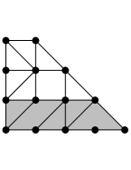
Figure 8. A $((1,1),(1))$-tangent curve $C$ to a tropical divisor $D$. All point conditions are in a small vertical strip, $p_{1}$ is far from all other points. The curve $C$ decomposes into the “upper” part $C^{\prime}$ and the “lower” part containing $p_{1}$. $C^{\prime}$ is $((0),(3))$-tangent to $D$. $C$ and $C^{\prime}$ have $\delta=2$ and $\delta^{\prime}=1$ as can be see from the dual subdivision on the right. The shaded part of the polygon is the difference between the degree $\Delta$ of $C$ and $\Delta^{\prime}$ of $C^{\prime}$.

Proof.

Our proof follows closely and extends the argument of Gathmann and Markwig’s proof of their [11, Theorem 4.3], where they proved this result in the non-refined case (i.e., $y=1$) for the surface $S={\mathbb{P}}^{2}$. Instead of points in a horizontal strip, we consider points in a vertical strip. The Gathmann-Markwig proof rests on an observation of Mikhalkin [20, Lemma 4.20] that holds for any toric surface. We use it in generalizing their argument.

Fix a small ${\varepsilon}>0$ and a large real number $M$. Consider a tropical generic point configuration $\Pi=\{p_{1},p_{2},\dots,p_{n}\}$ such that

1. the $x$-coordinates of all $p_{i}$ (including those on the divisor $D$) are within the interval $(-{\varepsilon},{\varepsilon})$,

2. the point $p_{1}$ is not on the divisor $D$ but its $y$-coordinate is less than $-M$,

3. all points $p_{i}\neq p_{1}$ not lying on $D$ have $y$-coordinate in the interval $(-{\varepsilon},{\varepsilon})$.

Let $C$ be a tropical curve of degree $\Delta$ with $\delta$ nodes. Then $C$ is of the following form:

1. all vertices of $C$ have $x$-coordinate in $(-{\varepsilon},{\varepsilon})$,

2. there are constants $a$ and $b$, depending only on $\Delta$, with $-N<a<b<-{\varepsilon}$ so that $C$ has no vertices in the strip ${\mathbb{R}}\times[a,b]$; all edges in this strip are vertical.

See Figure 8 for an illustration. This follows directly from the verbatim argument in [11]; note that their argument rests on [20, Lemma 4.20] which applies to arbitrary $\Delta$, so in particular to $S={\mathbb{P}}(1,1,m)$ and $S=\Sigma_{m}$.

There are two cases:

1. Case 1: $p_{1}$ lies on a vertical edge with weight $k\geq 1$. Then all edges of $C$ with $y$-coordinates $\leq-{\varepsilon}$ are vertical by the Gathmann-Markwig argument. We can move $p_{1}$ down onto the divisor $D$ and obtain a tropical curve with one more “fixed” tangency conditions. The weight of $C$ is $[k]_{y}$ times the weight of this new curve. The total contribution of tropical curves through $\Pi$ with $p_{1}$ on a vertical edge is thus

   $$\sum_{k:\beta_{k}>0}[k]_{y}\cdot N^{\Delta,\delta}(\alpha+e_{k},\beta-e_{k})(y).$$

2. Case 2: $p_{1}$ does not lie on a vertical half-ray. Then $C$ can be broken into two pieces: let $C^{\prime}$ be the curve with bounded edges in the vicinity of the points $p_{2},\dots,p_{n}$ that do not lie on $D$. The other piece, containing $p_{1}$, consists of the bounded edges of $C$ in the vicinity of $p_{1}$, one unbounded edge in direction $(-1,0)$ and $(1,m)$, respectively, and some vertical edges. See Figure 8 for an illustration of this decomposition. By construction, the degree $\Delta^{\prime}$ of $C^{\prime}$ is the lattice polygon obtained from $\Delta$ by removing a horizontal strip of width one at the bottom of $\Delta$.

   Next, we determine in how many ways $C^{\prime}$ can be extended to a tropical curve of degree $\Delta$ that is $(\alpha,\beta)$-tangent to the divisor $D$ and passes through $\Pi$. We know that $C^{\prime}$ is $(\alpha^{\prime},\beta^{\prime})$ tangent to $D$, for some $\alpha^{\prime}\leq\alpha$ and $\beta^{\prime}\geq\beta$. There are $\binom{\alpha}{\alpha^{\prime}}$ ways to choose which vertical edges of $C$ through a point in $\Pi\cap D$ belong to $C^{\prime}$. Similarly, there are are $\binom{\beta^{\prime}}{\beta}$ ways to choose which vertical edges of $C^{\prime}$ intersecting $D$ but not containing a point in $\Pi$ belong to $C$ (for more details see [11]).

   To show that the tangency conditions $\alpha^{\prime}$ and $\beta^{\prime}$ satisfy $I\alpha^{\prime}+I\beta^{\prime}=H(L-H)$, recall that degree $\Delta^{\prime}$ of $C^{\prime}$ is the polygon obtained from $\Delta$ by removing from $\Delta$ the bottom strip of lattice width $1$. Furthermore, $I\alpha^{\prime}+I\beta^{\prime}$ equals the lattice length of the bottom edge of $\Delta^{\prime}$. We argue for each surface separately.

   1. $S={\mathbb{P}}^{2}$: Here $H$ is the class of a line and $L$ is the class of a degree $d$ curve. Thus, we have $H(L-H)=d-1$, the length of the bottom edge of $\Delta^{\prime}$.

   2. $S=\Sigma_{m}$: In this case, we defined $H$ as the class of a section with $H^{2}=m$. Then $H(L-H)=c+(d-1)m$. Recall that $\Delta=\operatorname{conv}((0,0),(0,d),(c,d),(c+dm,0))$. The bottom edge of $\Delta^{\prime}$ has lattice length $c+(d-1)m=H(L-H)$.

   3. $S={\mathbb{P}}(1,1,m)$: Here $H$ is the class of a line, and we have $H(L-H)=(d-1)m$. As $\Delta=\operatorname{conv}((0,0),(0,d),(dm,0))$, $H(L-H)$ is precisely the lattice length of $\Delta^{\prime}$.

   Next, we relate the the $y$-multiplicities of $C$ and $C^{\prime}$. We have

   $$\operatorname{mult}(C;y)=\prod\limits_{i\geq 1}\left([i]_{y}\right)^{\alpha_{i}-\alpha^{\prime}_{i}+\beta^{\prime}_{i}-\beta_{i}}\operatorname{mult}(C^{\prime};y)$$

   and, therefore,

   $$\operatorname{mult}_{\alpha,\beta}(C;y)=\frac{1}{\prod_{i\geq 1}([i]_{y})^{\alpha_{i}}}\operatorname{mult}(C;y)=\prod\limits_{i\geq 1}([i]_{y})^{\beta^{\prime}_{i}-\beta_{i}}\operatorname{mult}_{\alpha^{\prime},\beta^{\prime}}(C^{\prime};y).$$

   Now, we show that the cogenus $\delta^{\prime}$ of $C^{\prime}$ satisfies

   $$\delta-\delta^{\prime}=I\alpha^{\prime}+I\beta^{\prime}-|\beta^{\prime}-\beta|.$$

   By definition, $\delta-\delta^{\prime}$ counts the number of parallelograms in the horizontal bottom strip of width $1$ in the dual subdivision $\Delta_{C}$. This number equals the number of unbounded edges of $C^{\prime}$ that intersect $D$ and are unbounded in $C$. But this number is precisely the length of the upper edge of the width $1$ strip minus the number of edges of $C^{\prime}$, that become bounded as edges in $C$, and thus equals $I\alpha^{\prime}+I\beta^{\prime}-|\beta^{\prime}-\beta|$.

   The recursive formula now follows: by the balancing condition, the $(\alpha^{\prime},\beta^{\prime})$-tangent curve $C^{\prime}$ can be completed to a $(\alpha,\beta)$-tangent curve $C$ with $p_{1}\in C\backslash C^{\prime}$ in a unique way, once we choose which vertical edges of $C$ through a point in $\Pi\cap D$ belong to $C^{\prime}$ and which vertical edges of $C^{\prime}$ intersecting $D$ but not containing a point in $C$ belong to $C$ (giving $\binom{\alpha}{\alpha^{\prime}}\cdot\binom{\beta^{\prime}}{\beta}$ choices).

Checking the initial conditions is trivial. ∎

Remark 7.6.

Note that in the case of rational ruled surfaces $\Sigma_{m}$, the above proof works also if we allow $m$ to be negative. Then $\Sigma_{m}=\Sigma_{-m}$, but with the role of $E$ and $H$ exchanged (this corresponds to exchanging the top and the bottom edge of $\Delta$). Expressed on $\Sigma_{m}$, the proof thus also shows the recursion (2.7), with the same initial conditions, but everywhere with $H$ replaced by $E$ and $\alpha$, $\beta$ specifying contacts along $E$ instead along $H$.

7.1. Refined Relative Node Polynomials for Plane Curves

We now extend the floor diagram technique to refined relative Severi degree for $S={\mathbb{P}}^{2}$. Then we show a polynomiality result (Theorem 7.8) about refined relative Severi degrees of ${\mathbb{P}}^{2}$, refining the result of [4, Theorem 1.1]. We expect a similar, more technical argument to work also for $S=\Sigma_{m}$ and $S={\mathbb{P}}(1,1,m)$, but restrict ourselves to ${\mathbb{P}}^{2}$ for simplicity. The following definitions are a quite straightforward refinement of [10, Section 3.2].

As we are only concerned with $S={\mathbb{P}}^{2}$, we denote by $\operatorname{{\bf FD}}(d,\delta)$ the set of $\Delta$-floor diagrams with $\Delta=\operatorname{conv}((0,0),(0,d),(d,0))$ and cogenus $\delta$, for any $d\geq 1$. Also, let $\operatorname{{\bf FD}}_{\text{conn}}(d,\delta)$ denote the collection of connected such floor diagrams. Let $\alpha$ and $\beta$ be two sequences of non-negative integers with only finitely many non-zero entries.

To each floor diagram ${\mathcal{D}}\in\operatorname{{\bf FD}}(d,\delta)$, there is a statistic $\nu_{\alpha,\beta}({\mathcal{D}})$, counting the number of “$(\alpha,\beta)$-markings” of ${\mathcal{D}}$ as in the non-relative case. The precise definition is given in [4, Definition 2.3], a reformulation of [10, Definition 3.13]. Intuitively, $\nu_{\alpha,\beta}({\mathcal{D}})$ counts the number of tropical curves of degree $\Delta$ that

1. are $(\alpha,\beta)$-tangent to $D=\{y=const\}$, where $const<<0$ (so $D$ is a very far down horizontal line),

2. “correspond” to the floor diagram ${\mathcal{D}}$ (in the sense of [10, Theorem 3.17]), and

3. that pass through a vertically stretched point configuration.

The refined relative Severi degree of ${\mathbb{P}}^{2}$ can be expressed purely combinatorially in terms of the $y$-weighted floor diagrams of Section 5: To simplify the formula, define (cf., [10, (3.6)]) for the unrefined setting)

$$\operatorname{mult}_{\beta}({\mathcal{D}},y)=\prod_{i\geq 1}([i]_{y})^{\beta_{i}}\cdot\operatorname{mult}({\mathcal{D}},y).$$

Proposition 7.7.

1. For any $d\geq 1$ and $\delta\geq 1$, the refined relative Severi degree of ${\mathbb{P}}^{2}$ is given by

   $$N^{d,\delta}(\alpha,\beta)(y)=\sum_{{\mathcal{D}}\in\operatorname{{\bf FD}}(d,\delta)}\operatorname{mult}_{\beta}({\mathcal{D}},y)\cdot\nu_{\alpha,\beta}({\mathcal{D}}).$$

2. For any $d\geq 1$ and $\delta\geq 1$, the refined irreducible relative Severi degree of ${\mathbb{P}}^{2}$ is computed by

   $$N^{d,\delta}_{0}(\alpha,\beta)(y)=\sum_{{\mathcal{D}}\in\operatorname{{\bf FD}}_{\text{conn}}(d,\delta)}\operatorname{mult}_{\beta}({\mathcal{D}},y)\cdot\nu_{\alpha,\beta}({\mathcal{D}}).$$

Proof.

We first prove Part 2. We may assume, by Theorem 7.3, that the tropical point configuration is vertically stretched. By [10, Theorem 3.17], there is a bijection $f$ between irreducible tropical curves of degree $d$ and cogenus $\delta$ that are $(\alpha,\beta)$-tangent to $D$ and $(\alpha,\beta)$-marked floor diagrams ${\mathcal{D}}$ with ${\mathcal{D}}\in\operatorname{{\bf FD}}_{\text{conn}}(d,\delta)$, where we used that these tropical curves have genus $g=\binom{d-1}{2}-\delta$. By [10, Theorem 3.17] (see also [10, Theorem 3.7] for the non-relative case but with more details), the map $f$ preserves the unrefined multiplicity ($y=1$) for any such tropical curve $C$ with corresponding floor diagram ${\mathcal{D}}$:

$$\operatorname{mult}_{\alpha,\beta}(C,1)=\operatorname{mult}_{\beta}({\mathcal{D}},1).$$

By definition of the refined multiplicities of tropical curves and floor diagrams (Definitions 3.5 and 5.2 and Equation (7.1)), the bijection $f$ preserves also the refined multiplicities:

$$\operatorname{mult}_{\alpha,\beta}(C,y)=\operatorname{mult}_{\beta}({\mathcal{D}},y),$$

as $\frac{1}{\prod_{i\geq 1}([i]_{y})^{\alpha_{i}}}\operatorname{mult}(C,y)=\prod_{i\geq 1}([i]_{y})^{\beta_{i}}\cdot\operatorname{mult}({\mathcal{D}},y)$, and Part 2 follows.

Part 1 follows from Part 2 by a straightforward refined extension of the inclusion-exclusion procedure of [10, Section 1] that was used to conclude [10, Corollary 1.9] (the non-relative unrefined count of reducible curves via floor diagrams) from [10, Theorem 1.6] (the non-relative unrefined count of irreducible curves via floor diagrams). ∎

Theorem 7.8.

For any $\delta\geq 1$, there is a polynomial

$$N_{\delta}(\alpha;\beta;y)\in{\mathbb{Q}}[y^{\pm 1}][\alpha_{1},\dots,\alpha_{\delta};\beta_{1},\dots,\beta_{\delta}]$$

in $\alpha_{i}$ and $\beta_{i}$ with coefficients in ${\mathbb{Q}}[y^{\pm 1}]$ such that, for any $\alpha$ and $\beta$ with $|\beta|\geq\delta$, we have

$$N^{d,\delta}(\alpha;\beta)(y)=\prod_{i\geq 1}([i]_{y})^{\beta_{i}}\frac{(|\beta|-\delta)!}{\beta_{1}!\beta_{2}!\cdots}\cdot N_{\delta}(\alpha;\beta;y).$$

The coefficients of the polynomial $N_{\delta}(\alpha;\beta;y)$ are preserved under the transformation $y\leftrightarrow y^{-1}$.

We call $N_{\delta}(\alpha;\beta;y)$ the refined relative node polynomial of ${\mathbb{P}}^{2}$.

Proof.

The proof is identical to the non-refined argument in [4, Theorem 1.1] but with the unrefined multiplicity of a floor diagram replaced by the refined multiplicity of the present paper. ∎

References

- [1] F. Ardila and F. Block, Universal polynomials for Severi degrees of toric surfaces, Adv. Math. 237 (2013), 165–193.
- [2] D. N. Bernstein, The number of roots of a system of equations, Funkcional. Anal. i Priložen. 9 (1975), no. 3, 1–4.
- [3] F. Block, Computing node polynomials for plane curves, Math. Res. Lett. 18 (2011), 621–643.
- [4] by same author, Relative node polynomials for plane curves, J. Algebraic Combin. 36 (2012), no. 2, 279–308.
- [5] E. Brugallé, Personal communication, 2013.
- [6] E. Brugallé and G. Mikhalkin, Enumeration of curves via floor diagrams, C. R. Math. Acad. Sci. Paris 345 (2007), no. 6, 329–334.
- [7] by same author, Floor decompositions of tropical curves: the planar case, Proceedings of Gökova Geometry-Topology Conference 2008, Gökova Geometry/Topology Conference (GGT), Gökova, 2009, pp. 64–90.
- [8] L. Caporaso and J. Harris, Counting plane curves of any genus, Invent. Math. 131 (1998), no. 2, 345–392.
- [9] P. Di Francesco and C. Itzykson, Quantum intersection rings, The moduli space of curves (Texel Island, 1994), Progr. Math., vol. 129, Birkhäuser Boston, Boston, MA, 1995, pp. 81–148.
- [10] S. Fomin and G. Mikhalkin, Labeled floor diagrams for plane curves, J. Eur. Math. Soc. (JEMS) 12 (2010), no. 6, 1453–1496.
- [11] A. Gathmann and H. Markwig, The Caporaso-Harris formula and plane relative Gromov-Witten invariants in tropical geometry, Math. Ann. 338 (2007), 845–868, arXiv:math.AG/0504392.
- [12] E. Getzler, Intersection theory on and elliptic Gromov-Witten invariants, J. Amer. Math. Soc. 10 (1997), no. 4, 973–998.
- [13] L. Göttsche, A conjectural generating function for numbers of curves on surfaces, Comm. Math. Phys. 196 (1998), no. 3, 523–533.
- [14] L. Göttsche and V. Shende, Refined curve counting on complex surfaces, arXiv:1208.1973, 2012.
- [15] by same author, The genera of relative Hilbert schemes for linear systems on Abelian and K3 surfaces, arXiv:1307.4316, 2013.
- [16] I. Itenberg, V. Kharlamov, and E. Shustin, A Caporaso-Harris type formula for Welschinger invariants of real toric del Pezzo surfaces, Comment. Math. Helv. 84 (2009), no. 1, 87–126.
- [17] I. Itenberg and G. Mikhalkin, On Block-Göttsche multiplicities for planar tropical curves, Int. Math. Res. Not. IMRN (2013), no. 23, 5289–5320, arXiv:1201.0451.
- [18] S.L. Kleiman and V. Shende, On the Göttsche Threshold. With an appendix by Ilya Tyomkin, A celebration of algebraic geometry, Clay Math. Proc., vol. 18, Amer. Math. Soc., Providence, RI, 2013, arXiv:1204.6254, pp. 429–449.
- [19] M. Kool, V. Shende, and R. P. Thomas, A short proof of the Göttsche conjecture, Geom. Topol. 15 (2011), 397–406.
- [20] G. Mikhalkin, Enumerative tropical geometry in , J. Amer. Math. Soc. 18 (2005), 313–377.
- [21] R. Pandharipande and R. P. Thomas, Stable pairs and BPS invariants, J. Amer. Math. Soc. 23 (2010), no. 1, 267–297.
- [22] Bruce E. Sagan, The cyclic sieving phenomenon: a survey, Surveys in combinatorics 2011, London Math. Soc. Lecture Note Ser., vol. 392, Cambridge Univ. Press, Cambridge, 2011, pp. 183–233. MR 2866734
- [23] E. Shustin, A tropical approach to enumerative geometry, Algebra i Analiz 17 (2005), no. 2, 170–214.
- [24] J. Steiner, Elementare Lösung einer geometrischen Aufgabe, und über einige damit in Beziehung stehende Eigenschaften der Kegelschnitte, J. Reine Angew. Math. 37 (1848), 161–192.
- [25] Y.-J. Tzeng, A proof of Göttsche-Yau-Zaslow formula, J. Differential Geom. 90 (2012), no. 3, 439–472.
- [26] R. Vakil, Counting curves on rational surfaces, Manuscripta Math. 102 (2000), no. 1, 53–84.