Stimulated Brillouin Scattering in integrated photonic waveguides: forces, scattering mechanisms and coupled mode analysis

Abstract

Recent theoretical studies of Stimulated Brillouin Scattering (SBS) in nanoscale devices have led to an intense research effort dedicated to the demonstration and application of this nonlinearity in on-chip systems. The key feature of SBS in integrated photonic waveguides is that small, high-contrast waveguides are predicted to experience powerful optical forces on the waveguide boundaries, which are predicted to further boost the SBS gain that is already expected to grow dramatically in such structures because of the higher mode confinement alone. In all recent treatments, the effect of radiation pressure is included separately from the scattering action that the acoustic field exerts on the optical field. In contrast to this, we show here that the effects of radiation pressure and motion of the waveguide boundaries are inextricably linked. Central to this insight is a new formulation of the SBS interaction that unifies the treatment of light and sound, incorporating all relevant interaction mechanisms — radiation pressure, waveguide boundary motion, electrostriction and photoelasticity — from a rigorous thermodynamic perspective. Our approach also clarifies important points of ambiguity in the literature, such as the nature of edge-effects with regard to electrostriction, and of body-forces with respect to radiation pressure. This new perspective on Brillouin processes leads to physical insight with implications for the design and fabrication of SBS-based nanoscale devices.

I Introduction

Stimulated Brillouin Scattering (SBS) is a nonlinear process by which light interacts coherently with acoustic vibrations in an optically transparent medium Boyd2003 . Predicted by Brillouin in 1922 Brillouin1922 , SBS was first experimentally demonstrated by Chiao, Townes and Stoicheff soon after the invention of the laser Chiao1964 , and thereafter became one of the standard techniques for measuring the mechanical properties of materials at high frequencies Uchida1973 . SBS has historically often been regarded as a non-desirable side-effect that must be either suppressed or accommodated, for example in fiber optics, where it can strongly deplete narrow-band pumps. However in recent years there has been a remarkable resurgence of interest in guided wave SBS EggletonBenjaminJ.2013 , driven largely by the ability to harness the effect in modern nanophotonics experiments Dainese2006 ; Tomes2009 ; Grudinin2010 ; Pant2011 ; Lee2012 . As well as forming the basis for the investigation of fundamental physical effects such as slow-light Thevenaz2008 and non-reciprocity Huang2011 , these experiments have led to a number of interesting SBS-based applications, such as narrow-linewidth tunable sources Abedin2012 , as well as on-chip processing of optical Pant2012a and radio-frequency Vidal2007 ; Chin2010 signals. SBS is closely related to the field of opto-mechanics Laer2015 , which is a similarly dynamic aera of research Papp2014 .

The SBS interaction arises from a pair of physical mechanisms that transfer energy back and forth between the electromagnetic field and the mechanical stresses and strains of the material Boyd2003 ; Kobyakov2010 . These mechanisms can be categorized as scattering (or forward-action) processes, by which the acoustic modes scatter light from one state to another, and back-action (or force-like) processes, by which the optical field generates mechanical motion via optical forces and pressures. Informed by the understanding of fiber and bulk systems, it was thought until very recently that SBS was driven entirely by the photoelasticity and electrostriction. These are inverse scattering and back-action processes respectively, linked by the thermodynamics of dielectric materials under mechanical strain. However these mechanisms are not the only possibilities for optomechanical interaction: in particular in the field of nano-optomechanics it is known that the back-action of radiation pressure can be very large in small, high-refractive-index-contrast devices, with the effect playing a central role in the interaction between optical and acoustic resonators in a number of seminal experiments in this fieldSchliesser2006 ; Grudinin2009 ; Lee2012 ; Eichenfield2009 . In recent work Rakich et al. Rakich2012 showed that radiation pressure can also make a significant contribution to the SBS gain: this is the result of large optical forces that act on the boundaries of suspended waveguides and resonantly excite acoustic modes of the free-standing structure. This prediction has important implications for the harnessing of SBS in CMOS-compatible materials such as silicon, in which electrostriction is relatively weak. Radiation pressure is strongest for small, high index contrast waveguides, and radiation-pressure-induced SBS has recently been observed in a silicon/silicon nitride hybrid waveguide Rakich2013 .

In this recent work and in the associated literature Rakich2012 ; Rakich2010 ; Qiu2012 , the scattering of the optical mode by the acoustic field is not considered directly; instead the phonon generation rate is computed by summing the optical forces due to both radiation pressure and electrostriction acting on the waveguide, and the SBS gain is then obtained via particle conservation in the classical limit. While this is a valid approach, there are several subtleties that arise in the physics that are not explicitly discussed in the existing literature. The main difficulty with this force-based approach is that force-like terms arise in such a way as to make it unclear whether they should be included or not. In SBS this is most clearly manifested in the form of an electrostrictive pressure term that appears on the boundary Rakich2013 : it is not entirely obvious whether this pressure term should be separately included, or whether it is simply a manifestation of the radiation pressure and already contained in the divergence of Maxwell’s stress tensor across a material boundary. In a similar way, the radiation pressure can appear to give rise to a body force Rakich2010 ; Rakich2012 in addition to the familiar surface terms, and it is unclear whether this body force should be included separately or whether it is readily contained in the electrostrictive process. These questions are not easy to answer; indeed the appropriate separation of optical forces in materials is related to the proper form of the photon momentum within material, and this has been a realm of some debate (known as the Abraham-Minkowski controversy) for the past hundred years. Given this uncertainty, the question arises not only as to which forces to include in one’s calculations, but whether there exist further force-like terms that are yet to be discovered.

Our approach to resolve these issues is to avoid optical forces as much as possible and found our description on the forward-action processes, which are not controversial. These processes include the scattering of light via the photo-elastic effect, scattering due to deformations of the waveguide boundary, as well as any other process whereby mechanical motion can influence the electromagnetic field. Furthermore, the forward-action half of the SBS interaction is important for any experiment in which the stimulated acoustic wave acts on other optical fields that are also present in the waveguide, as occurs in the generation of frequency combs via SBS Buettner2014 or in SBS-based optical isolation poulton2012design . Perhaps more critically, scattering mechanisms form an important part of the physics of SBS, and a theory that discusses these explicitly can not only shed light on the physicality of back-action processes, but is necessary to complete our understanding of Brillouin processes in integrated photonic waveguides.

Here we present a new formalism for SBS that considers all interactions in a unified way. By considering scattering mechanisms explicitly, we derive expressions for the interaction that do not rely on the exact form of the optical forces between and within materials. A main result of this formalism is the classification of forward and back-action processes into interaction pairs: for example we show that motion of the waveguide boundary forms the inverse process to the radiation pressure between lossless dielectrics, just as the photoelastic effect is associated with the electrostrictive force. We also identify a new term in the SBS interaction that results from coupling between the moving dielectric and the magnetic part of the optical mode. Furthermore, we observe that optical losses are related to irreversible forces using the case of radiation pressure as an example; this breaks the aforementioned symmetry between the scattering and back-action processes. Finally, we derive coupled mode equations that include all of these effects in a consistent framework. To the best of our knowledge this is the first such treatment in the literature.

The manuscript is structured as follows: In Section II, we state the properties of the systems under investigation and the expansion bases for the optical and acoustic wave propagation. In Section III, we formulate a conventional modal expansion and, more importantly, state the terms that describe the three scattering mechanisms of optical modes due to an acoustic displacement field in the waveguide’s bulk, on its surface and due to by the acoustic velocity field. These are all first-order terms that are present under our preliminaries. In Section IV, we again formulate a conventional modal expansion and then show based on a Lagrangian picture that for reversible interactions–and only for those–the coupling constant for the excitation of acoustic modes coincides with the previously formulated optical scattering constant. This provides a complete description of SBS that is independent of expressions for the optical forces and, hence, independent of the Abraham-Minkowski controversy. In Section V finally, we show how to derive the common resonant expression for the SBS-gain of a long waveguide and state limits for its applicability, we show that the coupled mode model as presented conserves energy and finally we discuss how the acousto-optic expressions that arise from our treatment are compatible with an expression for the optical momentum fluxes. In this context, we also explicitly comment on electrostrictive surface pressures.

II Preliminaries

We consider the interaction between optical and acoustic fields in waveguides having the general form depicted in Fig. 1, with a material cross section that is invariant along the $z$-axis. We make no assumptions on the shape of the waveguide, save that it is capable of guiding light in at least one optical mode. For the materials we assume the absence of magnetic response ($\mu_{r}=1$) and we disregard loss and dispersion in the dielectric parameters. We do so mainly to simplify the disucssion in Section IV.2; the effect of dispersion and loss on the optical pulse shape can be easily incorporated in the same way as we introduce acoustic loss in Section IV. Furthermore, we neglect the effect of any nonlinearity apart from the Brillouin scattering process that we investigate; specifically, we exclude piezoelectric materials. The exclusion of material dispersion is justified by the very small frequency shifts that occur in SBS, which are typically of only a few GHz. A material whose permittivity changes appreciably over this frequency range would probably be too lossy to be used as a material for a waveguide. If desired, weak dielectric loss can be incorporated in the mode expansion in the same way as we incorporate weak acoustic loss (see Section IV). Throughout this work, we use SI units.

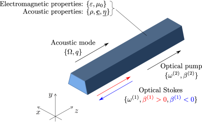
Figure 1: Schematic of the forward (Stokes field represented by the red arrow) and backward (Stokes field in blue) SBS interactions in a waveguide aligned along the $z$-axis. Although a specific waveguide cross-section is shown here, the results apply to waveguides of arbitrary cross section and composition.

II.1 Electromagnetic part

We describe the evolution of the optical fields by the electromagnetic wave equation in terms of the electric field

$$\nabla\times\nabla\times{\bf{E}}=-\mu_{0}\partial_{t}^{2}{\bf{D}};\quad{\bf{D}}=\varepsilon{\bf{E}};\quad\varepsilon=\varepsilon_{r}\varepsilon_{0}.$$ (1)

Here, ${\bf{E}}$ and ${\bf{D}}$ are the electric field and electric induction field respectively, and $\partial_{t}$ denotes the partial derivative with respect to time. In the context of acousto-optics, we prefer the term “electric induction field” over “electric displacement field” to avoid confusion with the mechanical displacement field. Later on, we also use the magnetic field ${\bf{H}}$. The dielectric function $\varepsilon({\bf{r}})=\varepsilon(x,y)$ is isotropic and homogeneous in the $z$-direction; ${\bf{r}}=(x,y,z)^{T}$ is the position vector. We assume that the electromagnetic fields can be approximated as a superposition of two propagating optical eigenmodes

$${\bf{E}}= {{\bf{E}}}^{(1)}+{{\bf{E}}}^{(2)},$$ (2)

where

$${{\bf{E}}}^{(i)}({\bf{r}},t)= {{\bf{e}}}^{(i)}({\bf{r}},t){a}^{(i)}(z,t)+{\rm{c.c.}}\ ,$$ (3)

and the mode functions factor as

$${{\bf{e}}}^{(i)}({\bf{r}},t)= {\widetilde{{\bf{e}}}}^{(i)}(x,y)\exp({\rm{i}}{\beta}^{(i)}z-{\rm{i}}{\omega}^{(i)}t),$$ (4)

with frequencies ${\omega}^{(i)}$ and wave vectors ${{\bf{k}}}^{(i)}=\hat{\rm z}{\beta}^{(i)}$. Note that the propagation constants ${\beta}^{(i)}$ may be both positive or negative. The dimensionless envelope functions ${a}^{(i)}$ are assumed to change only slowly over an optical wavelength and the time scale of an optical cycle. The other fields ${\bf{D}}$ and ${\bf{H}}$ are likewise expanded. The basis functions ${\widetilde{{\bf{e}}}}^{(i)}$ are bound solutions to the 2D-eigenproblem

$$(\nabla_{\!\!\perp}+{\rm{i}}\beta\hat{\rm z})\times(\nabla_{\!\!\perp}+{\rm{i}}\beta\hat{\rm z})\times\widetilde{{\bf{e}}}=\varepsilon\mu_{0}\omega^{2}\widetilde{{\bf{e}}},$$ (5)

where $\nabla_{\!\!\perp}$ is the nabla operator in the $x,y$-plane. There is no need to normalize these modes, although there may be practical advantages in doing so in numerical simulations. Since we neglect dispersion, the average electromagnetic energy density per unit length of the waveguide and the corresponding energy flux carried by the unnormalized mode functions are Jackson

$${{\mathcal{E}}}^{(i)}= 2\int{\rm{d}}^{2}r\ \varepsilon[{{\bf{e}}}^{(i)}]^{\ast}\cdot{{\bf{e}}}^{(i)};$$ (6)

$${{\mathcal{P}}}^{(i)}= 2\int{\rm{d}}^{2}r\ \hat{\rm z}\cdot([{{\bf{e}}}^{(i)}]^{\ast}\times{{\bf{h}}}^{(i)}),$$ (7)

where the integration is across the whole transverse plane. Using Maxwell’s equations, the latter can be recast to an expression that only involves the electric field; the energy transport velocity of the mode (which in the lossless case here is equal to its group velocity) Jackson is given by the ratio of the energy flux and energy densities:

$${{\mathcal{P}}}^{(i)}= \frac{1}{-{\rm{i}}{\omega}^{(i)}\mu_{0}}\int{\rm{d}}^{2}r\ \big{\{}[{{\bf{e}}}^{(i)}]^{\ast}\cdot[\hat{\rm z}\times(\nabla\times{{\bf{e}}}^{(i)})]$$

$$\quad+[{{\bf{e}}}^{(i)}]^{\ast}\cdot[\nabla\times(\hat{\rm z}\times{{\bf{e}}}^{(i)})]\big{\}}$$ (8)

$${v}^{(i)}= {{\mathcal{P}}}^{(i)}/{{\mathcal{E}}}^{(i)}.$$ (9)

II.2 Acoustic part

The fundamental equation for the mechanical part of the problem is the acoustic wave equation Auld1990 for the (mechanical) displacement field ${\bf{U}}$

$$-\rho\partial_{t}^{2}U_{i}+\sum_{jkl}\partial_{j}\left[c_{ijkl}+\eta_{ijkl}\partial_{t}\right]\partial_{k}U_{l}=-F_{i},$$ (10)

where $\rho$ is the density, ${\underline{\bf{c}}}$ is the stiffness tensor and ${\underline{\boldsymbol{\eta}}}$ is the viscosity tensor. Here, $\partial_{j}$ denotes the spatial derivative in the $j$-th spatial direction along $j$, where $j\in\{x,y,z\}$. The source term ${\bf{F}}$ on the right hand side is the driving external force field per unit volume through which the coupling to the electromagnetic field will be introduced. Assuming first that the acoustic losses are weak, we express the displacement field in terms of a solution ${\bf{u}}$ with carrier $\exp({\rm{i}}qz-{\rm{i}}\Omega t)$ to the lossless wave equation (i.e. with ${\underline{\boldsymbol{\eta}}}=0$) with a corresponding dimensionless envelope function $b$:

$${\bf{U}}({\bf{r}},t)= {\bf{u}}({\bf{r}},t)b(z,t)+{\rm{c.c.}}\ ;$$ (11)

$${\bf{u}}({\bf{r}},t)= \widetilde{{\bf{u}}}(x,y)\exp({\rm{i}}qz-{\rm{i}}\Omega t);$$ (12)

where $\widetilde{{\bf{u}}}$ is an eigenmode of the equation

$$\rho\Omega^{2}\widetilde{u}_{i}+\sum_{jkl}\ (\nabla_{\!\!\perp}+{\rm{i}}q\hat{\rm z})_{j}\ c_{ijkl}\ (\nabla_{\!\!\perp}+{\rm{i}}q\hat{\rm z})_{k}\ \widetilde{u}_{l}=0.$$ (13)

Note that we need not assume that the acoustic modes are strictly bound, since significant SBS can occur with leaky acoustic modes Poulton2013 . However, we assume that the acoustic propagation loss is small so that it appears to first approximation in the equation of motion for $b$. The first main advantage of this approach (i.e. moving the loss into the dynamics) is that the set of functions from which we choose ${\bf{u}}$ is formed by eigenfunctions to a Hermitian operator resulting in convenient orthogonality relations. Second, $|b|^{2}$ is related to the amplitude of the acoustic field in a straight-forward way throughout the whole system and so is directly related to the acoustic energy density. Again, there is no need to normalize the acoustic basis function. For what follows, the acoustic wave is chosen to be phase-matched with the beat between the two optical modes, i.e. we specify for the rest of this paper that

$$\Omega={\omega}^{(2)}-{\omega}^{(1)}\quad\quad\text{and}\quad\quad q={\beta}^{(2)}-{\beta}^{(1)}.$$ (14)

Note that such conditions are not in general automatically satisfied if the two electric fields are chosen freely. There must also be an appropriate resonant, phase-matched acoustic mode to provide the coupling. This strict phase-matching condition is used to select appropriate basis functions for the subsequent modal expansion.

The energy density of the acoustic field is the sum of the kinetic and the elastic energy. For a traveling wave, we focus on the time-averaged total energy per unit length of the waveguide Auld1990 . For an acoustic mode with unit envelope $b=1$ it thus reads

$${\mathcal{E}}_{b}= \frac{1}{2}\Big{\langle}\ {\int{\rm{d}}^{2}r\ \rho|\partial_{t}{\bf{U}}|^{2}+\sum_{ijkl}S_{ij}c_{ijkl}S_{kl}}\ \Big{\rangle}_{T_{\rm{ac}}}\ ,$$ (15)

where $S_{ij}=\frac{1}{2}(\partial_{i}U_{j}+\partial_{j}U_{i})$ is the strain tensor and the subscript $T_{\rm{ac}}$ indicates that the average is taken over a time window that is much longer than one acoustic cycle but shorter than the time scale for any relevant slower process. The transverse integral extends over the interior cross-section of the waveguide. If, as is typically the case, the waveguide’s total momentum and angular momentum are both zero, the average kinetic energy is equal to the average elastic energy and we may simplify:

$${\mathcal{E}}_{b}= \Big{\langle}\ {\int{\rm{d}}^{2}r\ \rho|\partial_{t}{\bf{U}}|^{2}}\ \Big{\rangle}_{T_{\rm{ac}}}=2\Omega^{2}\int{\rm{d}}^{2}r\ \rho|{\bf{u}}|^{2}\ .$$ (16)

The time-averaged energy flux that traverses the waveguide cross section ${\mathcal{P}}_{b}$ is given as the normal projection of the product between the velocity field and the stress tensor ${\underline{\bf{T}}}$ Auld1990 ; the mode’s energy transport velocity $v_{b}$ is defined as in Eq. (9):

$${\mathcal{P}}_{b}= -\Big{\langle}\ {\int{\rm{d}}^{2}r\ \hat{\rm z}\cdot(\partial_{t}{\bf{U}})\cdot{{\underline{\bf{T}}}}}\ \Big{\rangle}_{T_{\rm{ac}}}$$ (17)

$$= -2{\rm{i}}\Omega\int{\rm{d}}^{2}r\ \sum_{ikl}c_{zikl}u_{i}^{\ast}\partial_{k}u_{l};$$ (18)

$$v_{b}= {\mathcal{P}}_{b}/{\mathcal{E}}_{b}.$$ (19)

Finally, we assume that the coupling mechanism between optical and mechanical modes is reversible, i.e. that energy is lost only by the propagation of modes but not by the conversion between them. This means we neglect for example the optical force that occurs due to absorption of light. We comment on this in Section VI.

III Optical modal equations

In this section, we derive the equations of motion for the optical envelope functions ${a}^{(i)}$ and examine the two main effects by which a sound wave can scatter energy from one optical mode into the other.

III.1 Dynamic equations

The mechanical deformation affects the electromagnetic field in two ways. First, it changes the value of the permittivity. This is known as the photoelastic effect. Second, the material boundaries can be displaced and do work on the fields, an effect for which no familiar name seems to exist, but which we refer to as moving boundary scattering. In either case, the deformation leads to time-dependent changes $\Delta{\bf{E}}$, $\Delta{\bf{D}}$ in the electric field and induction, as illustrated by Fig. 2.

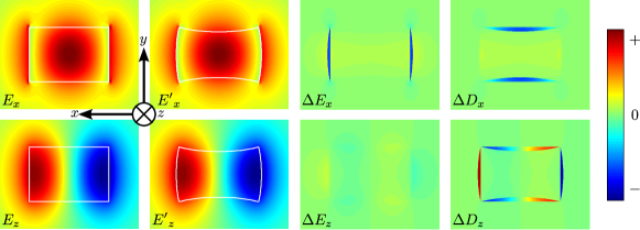
Figure 2: The two leftmost columns show the electric field distributions of an optical eigenmode in an rectangular waveguide (white outline) before and after a deformation. The other two columns show the deformation-related perturbations of the electric field and the electric induction. The waveguide deformation in this figure is grossly exaggerated for reasons of illustration. The color scale is linear and symmetric.

Furthermore, we allow for an additional magnetization $\Delta{\bf{H}}$ due to the motion of polarized particles. In formulating the problem in this way, we go beyond similar prior descriptions of SBS Huang2011 .

The distorted fields are still solutions of Maxwell’s equations and so satisfy the wave equation

$$\nabla\times\nabla\times({\bf{E}}+\Delta{\bf{E}})+\mu_{0}\partial_{t}^{2}({\bf{D}}+\Delta{\bf{D}})$$

$$\quad+\mu_{0}\partial_{t}\nabla\times\Delta{\bf{H}}=0.$$ (20)

The field perturbations contain contributions with all possible sum and difference frequencies, but only those perturbations that simultaneously match the spatial and temporal frequency of a basis function (i.e. are phase-matched to a basis function) are relevant for what follows. Thus, we neglect all but the phase-matched contributions

$$\Delta{\bf{E}}({\bf{r}},t)= {\Delta{\bf{e}}}^{(1)}({\bf{r}},t){a}^{(2)}(z,t)b^{\ast}(z,t)$$

$$\quad+{\Delta{\bf{e}}}^{(2)}({\bf{r}},t){a}^{(1)}(z,t)b(z,t)+{\rm{c.c.}}\ ,$$ (21)

Each one of the thus far unspecified patterns ${\Delta{\bf{e}}}^{(i)}$ contains the corresponding optical wave carrier:

$${\Delta{\bf{e}}}^{(i)}({\bf{r}},t)= {\widetilde{\Delta{\bf{e}}}}^{(i)}(x,y)\ \exp({\rm{i}}{\beta}^{(i)}z-{\rm{i}}{\omega}^{(i)}t),$$ (22)

The other field perturbations $\Delta{\bf{D}}$ and $\Delta{\bf{H}}$ are treated likewise. We have explicitly assumed that the field perturbations that are phase-matched to one optical mode stem from the interaction between the other optical mode and the sound wave and that they are linear in both fields. To proceed, we evaluate the contribution from the first mode to Eq. (20):

$$0= \nabla\times\nabla\times({a}^{(1)}{{\bf{e}}}^{(1)}+{a}^{(2)}b^{\ast}{\Delta{\bf{e}}}^{(1)})+\mu_{0}\partial_{t}^{2}({a}^{(1)}{{\bf{d}}}^{(1)}+{a}^{(2)}b^{\ast}{\Delta{\bf{d}}}^{(1)})+\mu_{0}\partial_{t}\nabla\times({a}^{(2)}b^{\ast}{\Delta{\bf{h}}}^{(1)})+{\rm{c.c.}}$$ (23)

$$= {a}^{(1)}\Big{[}\nabla\times\nabla\times{{\bf{e}}}^{(1)}+\mu_{0}\partial_{t}^{2}{{\bf{d}}}^{(1)}\Big{]}+\Big{[}\hat{\rm z}\times(\nabla\times{{\bf{e}}}^{(1)})+\nabla\times(\hat{\rm z}\times{{\bf{e}}}^{(1)})\Big{]}\partial_{z}{a}^{(1)}-2{\rm{i}}{\omega}^{(1)}\mu_{0}{{\bf{d}}}^{(1)}\partial_{t}{a}^{(1)}$$

$$\quad+{a}^{(2)}b^{\ast}\Big{[}\nabla\times\nabla\times{\Delta{\bf{e}}}^{(1)}+\mu_{0}\partial_{t}^{2}{\Delta{\bf{d}}}^{(1)}+\mu_{0}\partial_{t}\nabla\times{\Delta{\bf{h}}}^{(1)}\Big{]}+\ \text{h.o.t.}+{\rm{c.c.}}\ ,$$ (24)

where ‘h.o.t’ stands for higher order terms in the perturbations and higher order derivatives of the envelope functions. They are neglected since we assumed slowly varying envelopes. Next, we project onto the mode ${\bf{e}}_{1}$ and average over a time interval much longer than the optical time scale. In this average process, all complex conjugate terms disappear. Using Eqs. (8) and (9), and dropping all higher order terms, we obtain

$$-{\rm{i}}{\omega}^{(1)}\mu_{0}{{\mathcal{P}}}^{(1)}\partial_{z}{a}^{(1)}-{\rm{i}}{\omega}^{(1)}\mu_{0}{{\mathcal{E}}}^{(1)}\partial_{t}{a}^{(1)}$$

$$= {a}^{(2)}b^{\ast}\Bigg{\{}\int{\rm{d}}^{2}r\quad\Big{[}{{\bf{e}}}^{(1)}\Big{]}^{\ast}\cdot\Big{[}\mu_{0}\partial_{t}^{2}{\Delta{\bf{d}}}^{(1)}+\nabla\times\nabla\times{\Delta{\bf{e}}}^{(1)}+\partial_{t}\nabla\times{\Delta{\bf{h}}}^{(1)}\Big{]}\Bigg{\}}$$ (25)

$$= {a}^{(2)}b^{\ast}\mu_{0}\Bigg{\{}\int{\rm{d}}^{2}r\quad\Big{[}{{\bf{e}}}^{(1)}\Big{]}^{\ast}\cdot\Big{[}\partial_{t}^{2}{\Delta{\bf{d}}}^{(1)}\Big{]}-\Big{[}\partial_{t}^{2}{{\bf{d}}}^{(1)}\Big{]}^{\ast}\cdot{\Delta{\bf{e}}}^{(1)}+\mu_{0}\Big{[}\partial_{t}{{\bf{h}}}^{(1)}\Big{]}^{\ast}\cdot\partial_{t}{\Delta{\bf{h}}}^{(1)}\Bigg{\}}.$$ (26)

In the step from Eq. (25) to Eq. (25), we applied two partial integrations (with vanishing boundary terms due to the modes’ exponential localization) to transfer a double curl operation to the complex conjugate e-field, used the waveguide equation and one of Maxwell’s equations: $\nabla\times{\bf{E}}+\partial_{t}{\bf{B}}=0$. The second optical mode is treated likewise. We end up with the final equations for the optical envelope functions, where ${v}^{(1,2)}$ are the respective (potentially negative) group velocities:

$$\partial_{z}{a}^{(1)}+\frac{1}{{v}^{(1)}}\partial_{t}{a}^{(1)}= -\frac{{\rm{i}}{\omega}^{(1)}{a}^{(2)}b^{\ast}}{{{\mathcal{P}}}^{(1)}}Q_{1},$$ (27)

$$\partial_{z}{a}^{(2)}+\frac{1}{{v}^{(2)}}\partial_{t}{a}^{(2)}= -\frac{{\rm{i}}{\omega}^{(2)}{a}^{(1)}b}{{{\mathcal{P}}}^{(2)}}Q_{2}.$$ (28)

Here

$$Q_{1}= \int{\rm{d}}^{2}r\Big{[}[{{\bf{e}}}^{(1)}]^{\ast}\cdot{\Delta{\bf{d}}}^{(1)}$$

$$\quad-[{{\bf{d}}}^{(1)}]^{\ast}\cdot{\Delta{\bf{e}}}^{(1)}-\mu_{0}[{{\bf{h}}}^{(1)}]^{\ast}\cdot{\Delta{\bf{h}}}^{(1)}\Big{]},$$ (29)

$$Q_{2}= \int{\rm{d}}^{2}r\Big{[}[{{\bf{e}}}^{(2)}]^{\ast}\cdot{\Delta{\bf{d}}}^{(2)}$$

$$\quad-[{{\bf{d}}}^{(2)}]^{\ast}\cdot{\Delta{\bf{e}}}^{(2)}-\mu_{0}[{{\bf{h}}}^{(2)}]^{\ast}\cdot{\Delta{\bf{h}}}^{(2)}\Big{]},$$ (30)

are works per unit length associated with the couplings.

In a transparent solid insulator, the two effects that lead to the perturbations $\Delta{{\bf{e}}}^{(i)}$ and $\Delta{{\bf{d}}}^{(i)}$ are the common photoelastic effect and field perturbations caused by the changing continuity conditions when a dielectric interface is shifted. The perturbation $\Delta{{\bf{h}}}^{(i)}$ is caused by an effective dynamic magnetic coupling effect. We now discuss these in more detail.

III.2 Photoelastic effect

The term photoelasticity refers to the effect that the electric susceptibility of matter changes if it is subject to strain. In a solid and for small deformations, this can be phenomenologically described by a fourth rank tensor ${\underline{\bf{p}}}$. This tensor can be derived from quasi-static or acousto-optic experiments:

$$\chi^{(\rm{PE})}_{ij}=\varepsilon_{r}^{2}\sum_{kl}p_{ijkl}\partial_{k}U_{l},$$ (31)

where we have exploited the symmetry $p_{ijkl}=p_{ijlk}$ of the photoelastic tensor. From Eq. (31) follow the photoelastic parts of the overlap integrals in Eq. (27) and Eq. (28):

$$Q^{(\rm{PE})}_{1}= \int_{A}{\rm{d}}^{2}r\ [{{\bf{e}}}^{(1)}]^{\ast}\cdot{\Delta{\bf{d}}}^{(1,{(\rm{PE})})}$$ (32)

$$= \varepsilon_{0}\int_{A}{\rm{d}}^{2}r\ \sum_{ijkl}\varepsilon_{r}^{2}[{e_{i}}^{(1)}]^{\ast}{e_{j}}^{(2)}p_{ijkl}\partial_{k}u_{l}^{\ast},$$ (33)

where ${\Delta{\bf{d}}}^{(1,{(\rm{PE})})}$ is that part of the physical photoelastic polarization field $\Delta D^{(\rm{PE})}_{i}=\varepsilon_{0}E_{j}\chi_{ij}^{(\rm{PE})}({\bf{U}})$ that is phase-matched with the optical mode $[{{\bf{e}}}^{(1)}]^{\ast}$. By interchanging the optical mode labels, we find $Q^{(\rm{PE})}_{1}=[Q^{(\rm{PE})}_{2}]^{\ast}$. Again, the integral is only to be taken over the interior of the waveguide’s material cross section $A$. Although the displacement field is discontinuous at the waveguide boundary, the strain field goes from a finite value to zero and the photoelastic change of the permittivity remains finite. Boundary effects that are caused by a displacement of the material boundary are treated in Section III.4.

III.3 Moving polarization effect

It may be surprising that deformation can lead to a magnetic polarization in a body that was explicitly assumed to have no magnetic susceptibility. In fact, the absence of magnetic material response only guarantees that a static deformation cannot cause such an effect. A changing mechanical displacement field creates a temporary magnetic polarization that is proportional to the electric polarization, because the latter describes the dipole moment density of a microscopic charge separation. When the material is deformed, the separated charges are forced to move and form two separated, counter-directed microscopic currents that induce a magnetic field at the position of the moving dipole. This effect is discussed in the context of isolated (electric and magnetic) point-dipoles in Ref. Hnizdo2012 . In our case of continuous dipole distributions (i.e. polarization fields), the effective magnetic polarization is

$$\Delta{\bf{H}}= (\partial_{t}{\bf{U}})\times{\bf{P}},$$ (34)

where ${\bf{P}}={\bf{D}}-\varepsilon_{0}{\bf{E}}$ is the total electric polarization. The phase-matched terms are

$${\Delta{\bf{h}}}^{(1)}= {\rm{i}}\Omega\varepsilon_{0}(\varepsilon_{r}-1){\bf{u}}^{\ast}\times{{\bf{e}}}^{(2)},$$ (35)

and the overlap product with the magnetic induction field $\mu_{0}{\bf{h}}$ is after a permutation of the triple product:

$$Q^{(\rm{DP})}_{1}= {\rm{i}}\Omega\mu_{0}\varepsilon_{0}\int_{A}{\rm{d}}^{2}r\ (\varepsilon_{r}-1){\bf{u}}^{\ast}\cdot({{\bf{e}}}^{(2)}\times[{{\bf{h}}}^{(1)}]^{\ast}).$$ (36)

As before, a permutation of mode labels leads to $Q^{(\rm{DP})}_{1}=[Q^{(\rm{DP})}_{2}]^{\ast}$.

This term has not been well-appreciated in the recent literature on SBS. For optical modes that resemble plane waves, the magnetic induction field in the overlap integral Eq. (36) can be expressed in terms of the optical wave vector and the electric field (see Appendix A) and can be incorporated into the electric photoelastic tensor, where it appears as a dispersive, anti-symmetric contribution Nelson1971 . This is the situation e.g. in conventional optical fibers but clearly not in integrated waveguides such as silicon nanowires. As a consequence, care must be taken when predicting the SBS-coefficients of small waveguides using photoelastic tensor elements that were measured with high-frequency deformation fields e.g. in acousto-optic or SBS experiments. We will resume this discussion in Section V.3.

III.4 Boundary term

The second important coupling mechanism is caused by the displacement of the material interfaces of the waveguide as the sound wave propagates along it. This leads to a strong change in the fields over a very small area exactly at the waveguide surface. This is in contrast to the photoelastic effect, which causes small field changes over the full waveguide cross section. As a consequence, this effect becomes more relevant as the waveguide cross-sectional area is decreased.

Clearly, this type of field perturbation appears at every dielectric interface; between different solids or liquids and between condensed materials and gases or vacuum. For the sake of illustration, we discuss this using the example of a rectangular nanowire with permittivity $\varepsilon_{a}$ surrounded by a domain with another permittivity $\varepsilon_{b}$. Consider a section of the waveguide outline that is displaced outward as illustrated by Fig. 3. We choose the interface normal vector to point outwards. Maxwell’s equations require that the normal component of the induction field and the in-plane components of the electric fields are continuous across the interface. Thus, the electric and induction fields in the space between the old and the displaced boundary are modified according to

$${\bf{E}}^{(\text{before})}={\bf{E}}_{\parallel}+\varepsilon_{b}^{-1}\varepsilon_{0}^{-1}{\bf{D}}_{\perp}$$

$$\longrightarrow \quad{\bf{E}}^{(\text{after})}={\bf{E}}_{\parallel}+\varepsilon_{a}^{-1}\varepsilon_{0}^{-1}{\bf{D}}_{\perp},$$ (37)

$${\bf{D}}^{(\text{before})}=\varepsilon_{b}\varepsilon_{0}{\bf{E}}_{\parallel}+{\bf{D}}_{\perp}$$

$$\longrightarrow \quad{\bf{D}}^{(\text{after})}=\varepsilon_{a}\varepsilon_{0}{\bf{E}}_{\parallel}+{\bf{D}}_{\perp},$$ (38)

where the subscripts $\perp$ and $\parallel$ refer to the normal and the in-plane parts of the field vectors, respectively. Thus, we find for the field perturbations in this small area:

$$\Delta{\bf{E}}= (\varepsilon_{b}^{-1}-\varepsilon_{a}^{-1})\varepsilon_{0}^{-1}\hat{\rm n}(\hat{\rm n}\cdot{\bf{D}}),$$ (39)

$$\Delta{\bf{D}}= (\varepsilon_{a}-\varepsilon_{b})\varepsilon_{0}(-\hat{\rm n}\times\hat{\rm n}\times{\bf{E}}).$$ (40)

Essentially, this is the action of the deformation-related perturbation operator on the stress-free solution. These formulae have already been discussed at length by Johnson et al. in the context of perturbation theory for cavity eigenfrequencies Johnson2002 .

Assuming that the boundary displacement is so small that the field perturbations are homogeneous in the normal direction, we may replace the integration over the whole of the transverse plane in Eqs. (27) and (28) with a line integration only over all boundary contours $\mathcal{C}=\{\mathcal{C}_{i}\}$ of the waveguide cross section. In terms of time-harmonic wave patterns, we find for the coupling coefficients due to the moving boundary

$$Q_{1}^{{(\rm{MB})}}= \int_{\mathcal{C}}{\rm{d}}{\bf{r}}\ ({\bf{u}}^{\ast}\cdot\hat{\rm n})\Big{[}(\varepsilon_{a}-\varepsilon_{b})\varepsilon_{0}(\hat{\rm n}\times{{\bf{e}}}^{(1)})^{\ast}(\hat{\rm n}\times{{\bf{e}}}^{(2)})$$

$$\quad-(\varepsilon_{b}^{-1}-\varepsilon_{a}^{-1})\varepsilon_{0}^{-1}(\hat{\rm n}\cdot{{\bf{d}}}^{(1)})^{\ast}(\hat{\rm n}\cdot{{\bf{d}}}^{(2)})\Big{]},$$ (41)

where the factor $({\bf{u}}^{\ast}\cdot\hat{\rm n})$ is simply the distance by which the interface is displaced. Again, we find by re-labeling optical mode designators that $Q_{2}^{{(\rm{MB})}}=[Q_{1}^{{(\rm{MB})}}]^{\ast}$. Finally the total coupling in Eqs. (29) and (30) is the sum of the photoelastic and radiation pressure effects: $Q_{i}=Q_{i}^{{(\rm{PE})}}+Q_{i}^{{(\rm{DP})}}+Q_{i}^{{(\rm{MB})}}$. Among those, the photoelastic coupling effect is always relevant and dominates in extended systems such as fibers. The moving boundary effect can reach comparable magnitude in small high-index systems, as demonstrated by the Rakich group Rakich2012 ; Rakich2013 ; Rakich2010 . The moving polarization coupling is usually very weak as we show in Appendix A.

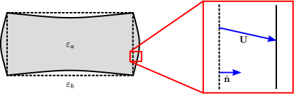
Figure 3: Sketch of the boundary displacement effect. A waveguide with dielectric permittivity $\varepsilon_{a}$ is embedded in a background material with permittivity $\varepsilon_{b}$. Please note that the deformation is grossly exaggerated in the left hand sketch. For surface displacements of realistic magnitude, the quasi-parallel shift of the interface by the distance $\hat{\rm n}\cdot{\bf{U}}$ is the dominant effect and the second order effects related to a change in the normal vector $\hat{\rm n}$ are negligible. This situation is shown in the close-up on the right hand side.

IV Acoustic modal equations

After our description of the dynamics of the optical envelope functions, we now turn to the acoustic part of the problem. First, we derive the dynamic equations and then show how the driving term is related to the respective driving terms of the optical modal equations already found Section III.

IV.1 Dynamic equations

We start with Eq. (10), where the driving force densities $F_{i}$ are due to the electromagnetic fields. In analogy to the driving terms in the optical wave equation, we assume that the phase-matched part of the driving force density ${\bf{F}}$ is linear in the two optical envelope functions:

$${\bf{F}}({\bf{r}},t)= {\bf{f}}({\bf{r}},t)[{a}^{(1)}(z,t)]^{\ast}{a}^{(2)}(z,t)+{\rm{c.c.}}\ .$$ (42)

Substituting this ansatz into equation (10) and dropping higher order terms eventually yields

$$-{\rm{i}}\Omega\sum_{jkl}\Big{[}(c_{izkl}\partial_{k}+\partial_{j}c_{ijzl})u_{l}\partial_{z}b-2{\rm{i}}\Omega\rho u_{i}\partial_{t}b$$

$$\quad+(\partial_{j}\eta_{ijkl}\partial_{k}u_{l})b+[{a}^{(1)}]^{\ast}{a}^{(2)}f_{i}\Big{]}+{\rm{c.c.}}=0.$$ (43)

After projecting onto the mode ${\bf{u}}$, we end up with the acoustic mode equation

$$\partial_{z}b+\frac{1}{v_{b}}\partial_{t}b+\alpha b= -\frac{{\rm{i}}\Omega[{a}^{(1)}]^{\ast}{a}^{(2)}}{{\mathcal{P}}_{b}}Q_{b}$$ (44)

$$\alpha= \frac{\Omega^{2}}{{\mathcal{P}}_{b}}\Bigg{\{}\int{\rm{d}}^{2}r\ \sum_{jkl}u_{i}^{\ast}\partial_{j}\eta_{ijkl}\partial_{k}u_{l}\Bigg{\}};$$ (45)

$$Q_{b}= \int{\rm{d}}^{2}r\ {\bf{u}}^{\ast}\cdot{\bf{f}},$$ (46)

where the coupling parameter $Q_{b}$ is again explicitly a work linear density, and $1/\alpha$ is the effective dissipation length for the acoustic mode. This approach to the acoustic part of the SBS process differs significantly from the treatment in previous works Rakich2010 ; Rakich2012 ; Rakich2013 . The main difference is the fact that we regard the sound field as a moving wave rather than a localized oscillator. In Section V.1 we show how to obtain expressions that are consistent with the literature by assuming that neither the optical nor the acoustic amplitude vary over the mean acoustic propagation length — an approximation that is well justified in long waveguides. In very short waveguides, however, the propagation of the sound wave can no longer be neglected and a treatment like ours is necessary.

Regarding the limitations of our treatment, it should be stressed that the slowly varying envelope approximation is not necessarily justified for the acoustic part of the problem, because it requires that the acoustic wavelength is much smaller than the length scale on which the envelope function varies. This means that $q$ has to be much larger than the damping constant $\alpha$, and the beat length $\pi/q$ much less than the free propagation length along the waveguide. This is usually the case for backward-SBS and forward-SBS between different branches of the optical dispersion relation unless they are nearly degenerate. However, an example for a SBS-setup where the SVEA (and therefore our equations) is formally not justified can be found in Ref. Rakich2013 . In this work, the waveguide consists of a series of forward-type SBS-active suspended regions with a length of $100\,\mu\rm{m}$ each. This is clearly the maximum free propagation length for the acoustic wave. The beat length between the optical modes, on the other hand, is given by the SBS Stokes shift and the optical phase velocity, leading to an acoustic wavelength of the order of centimeters. Here, the suspended regions resemble localized harmonic oscillators and a treatment along the lines of Ref. poulton2012design seems appropriate.

IV.2 Optical forces and thermodynamic considerations

We now come to a key part of the analysis, identifying the optical force density from the optical scattering integral Eq. (29). There are two common approaches to derive the force that is caused by an optical field. The first way is via the Lorentz force. To this end, the material response is expressed in terms of microscopic charges and currents which interact with the incident field. We basically follow this path in Section V.3. The second way is via a thermodynamic potential, see e.g. Ref. Feldman1975 for such a discussion of the connection between electrostriction and the photo-elastic effect. While less familiar in the photonics community, the latter approach is attractive for our problem, provided that the change in the entropy is known.

As part of our assumptions, we neglect optical loss and irreversible coupling effects. The only source of entropy is the mechanical loss, which can be neglected because of the very small acoustic amplitudes in SBS. If optical loss were to be included, the entropic contribution to the thermodynamic potential could become appreciable. However, the most common experimental situation is a steady state where temporally constant optical and acoustic intensities vary spatially along the waveguide. In this case, the temperature would approach an equilibrium distribution that can be controlled via the properties of a heat sink; the temperature is therefore the natural choice for an independent variable.

Typically, the mechanical contribution to the free energy of a solid body is separated into boundary terms (surface pressures) and interior density-like terms (internal stress) Landau7 . However, such a distinction is not convenient for our problem because of the complexity associated with the moving waveguide boundary. Accordingly, we adopt a picture based on a displacement field ${\bf{U}}$ and a driving force density field ${\bf{F}}$ that yields both body force densities and boundary pressures. Furthermore, the moving polarization effect depends on $\partial_{t}{\bf{U}}$, so a Lagrangian picture is best suited to the problem. Finally, the electromagnetic continuity conditions force us to decompose the electric fields in an unusual way.

The variation in the free energy density ${\mathcal{F}}$ of a waveguide satisfies

$$\delta\!{\mathcal{F}}=-S\delta\!T+\delta\!{\mathcal{E}}^{(\rm{mech})}+\delta\!{\mathcal{E}}^{(\rm{opt})},$$ (47)

where $\delta\!{\mathcal{E}}^{(\rm{mech})}$ and $\delta\!{\mathcal{E}}^{(\rm{opt})}$ are the changes in mechanical and optical energy, respectively, and $S$ and $T$ denote entropy per unit length and temperature. The latter are not of great importance in this context as we assume a thermodynamically inert process. We can therefore neglect them. For the two other terms we assume:

$${\mathcal{E}}^{(\rm{mech})}= \frac{\rho}{2}|\partial_{t}{\bf{U}}|^{2}+\Phi,$$ (48)

$${\mathcal{E}}^{(\rm{opt})}= \frac{1}{2}\Big{\langle}\ {{\bf{E}}\cdot{\bf{D}}+{\bf{H}}\cdot{\bf{B}}}\ \Big{\rangle}_{T_{\rm{opt}}},$$ (49)

where $\Phi({\bf{U}})$ is the stored elastic energy and (recognizing that the mechanical system cannot follow the rapid electromagnetic oscillations,) the electromagnetic energy density is averaged over a time window $T_{\text{opt}}$ that includes many optical cycles but is much smaller than one acoustic cycle. Note that in this context we distinguish between ${\bf{B}}$ and $\mu_{0}{\bf{H}}$, because we assign the effect of the sound wave to one of them (${\bf{H}}$) while the other one (${\bf{B}}$) is kept fixed as an independent variable. Next, we perform a Legendre transformation to obtain the Lagrangian for the opto-mechanical system. Here, it comes as a great convenience that the electric fields only depend on ${\bf{U}}$ (hence are potential-like) while the magnetic field only depends on $\partial_{t}{\bf{U}}$ and effectively provides a correction to the kinetic energy:

$${\mathcal{L}}= \frac{\rho}{2}(\partial_{t}{\bf{U}})^{2}-\Phi-\frac{1}{2}\Big{\langle}\ {{\bf{E}}\cdot{\bf{D}}-{\bf{B}}\cdot{\bf{H}}}\ \Big{\rangle}_{T_{\rm{opt}}}.$$ (50)

The first two terms lead to the acoustic wave equation, whereas the last two terms correspond to the optical driving force ${\bf{F}}$. By separating these two types of terms in the Euler-Lagrange equations, we find

$${\bf{F}}= \rho\partial_{t}^{2}{\bf{U}}+\frac{\partial\Phi}{\partial{\bf{U}}}$$ (51)

$$= -\frac{1}{2}\Big{\langle}\ {\frac{\partial({\bf{E}}\cdot{\bf{D}})}{\partial{\bf{U}}}}\ \Big{\rangle}_{T_{\rm{opt}}}$$

$$\quad-\frac{1}{2}\frac{{\rm{d}}}{{\rm{d}}t}\Big{\langle}\ {{\bf{B}}\cdot\frac{\partial{\bf{H}}}{\partial(\partial_{t}{\bf{U}})}}\ \Big{\rangle}_{T_{\rm{opt}}}\ .$$ (52)

At this stage it is not yet clear whether the electric part to the electromagnetic energy is best expressed with respect to the induction field or the electric field as the independent variable. The aim must be to formulate the optical field in terms that are not influenced by the mechanical displacement field and, thus, allow us to describe the optical power independently from the acoustic excitation. In fact, when the waveguide is deformed as described by ${\bf{U}}$, both ${\bf{E}}$ and ${\bf{D}}$ may be perturbed. A key observation, however, is that there is always a composition of field components of ${\bf{E}}$ and ${\bf{D}}$ that is not changed by the deformation. This is most easily seen for perturbations of any boundary between different dielectrics (see Section III.4). According to the continuity conditions, this unchanged composition consists of the normal part of ${\bf{D}}$ and the tangential part of ${\bf{E}}$; for the photoelastic effect, which can be described as a change in permittivity (see Section III.2), the unchanged quantity is ${\bf{E}}$. Such compositions of ${\bf{E}}$ and ${\bf{D}}$ are independent of the presence of a weak sound wave and determined only by the choice of the waveguide optical modes excited. We denote them with a subscript “${\rm{indep}}$”:

$$\frac{\partial{\bf{E}}_{\rm{indep}}}{\partial U_{i}}=\frac{\partial{\bf{D}}_{\rm{indep}}}{\partial U_{i}}= 0.$$ (53)

The dependent variables (subscript “${\rm{dep}}$”) then are what remains, i.e. the difference between perturbed fields and the independent parts:

$${\bf{E}}_{\rm{dep}}= {\bf{E}}+\Delta{\bf{E}}-{\bf{E}}_{\rm{indep}},$$ (54)

$${\bf{D}}_{\rm{dep}}= {\bf{D}}+\Delta{\bf{D}}-{\bf{D}}_{\rm{indep}}.$$ (55)

By construction, they completely contain the deformation-dependence of the optical fields:

$$\frac{\partial{\bf{E}}_{\rm{dep}}}{\partial U_{i}}=\frac{\partial\Delta{\bf{E}}}{\partial U_{i}};\quad\frac{\partial{\bf{D}}_{\rm{dep}}}{\partial U_{i}}=\frac{\partial\Delta{\bf{D}}}{\partial U_{i}}.$$ (56)

If we assume that the continuity conditions at material discontinuities determine the decomposition of the fields into dependent and independent quantities, we can furthermore say that

$${\bf{E}}_{\rm{indep}}\cdot{\bf{D}}_{\rm{indep}}={\bf{E}}_{\rm{dep}}\cdot{\bf{D}}_{\rm{dep}}=0.$$ (57)

This is also true for electrostriction, because in this case ${\bf{D}}_{\rm{indep}}={\bf{E}}_{\rm{dep}}=0$. In order to calculate the optical forces, we thus perform another Legendre transformation:

$$\tilde{\mathcal{L}}= {\mathcal{L}}-\Big{\langle}\ {\int{\rm{d}}^{2}r\ {\bf{E}}_{\rm{dep}}\cdot{\bf{D}}}\ \Big{\rangle}_{T_{\rm{opt}}}.$$ (58)

Its electric part satisfies the form

$$\Big{\langle}\ {\frac{\partial({\bf{E}}\cdot{\bf{D}})}{\partial{\bf{U}}}}\ \Big{\rangle}_{T_{\rm{opt}}}$$

$$= \Big{\langle}\ {\bf{E}}_{\rm{indep}}\cdot\frac{\partial{\bf{D}}_{\rm{dep}}}{\partial{\bf{U}}}-{\bf{D}}_{\rm{indep}}\cdot\frac{\partial{\bf{E}}_{\rm{dep}}}{\partial{\bf{U}}}$$

$$\quad+{\bf{E}}_{\rm{indep}}\cdot\frac{\partial{\bf{D}}_{\rm{indep}}}{\partial{\bf{U}}}-{\bf{D}}_{\rm{dep}}\cdot\frac{\partial{\bf{E}}_{\rm{indep}}}{\partial{\bf{U}}}\ \Big{\rangle}_{T_{\rm{opt}}}$$ (59)

$$= \Big{\langle}\ {{\bf{E}}\cdot\frac{\partial{\bf{D}}_{\rm{dep}}}{\partial{\bf{U}}}-{\bf{D}}\cdot\frac{\partial{\bf{E}}_{\rm{dep}}}{\partial{\bf{U}}}}\ \Big{\rangle}_{T_{\rm{opt}}}\ ,$$ (60)

where we used Eq. (57) in the second step. With this, the optical force density at position ${\bf{r}}$ with the illumination of the waveguide held constant becomes

$${\bf{F}}({\bf{r}})= \frac{1}{2}\Big{\langle}\ {{\bf{E}}\cdot\frac{\partial(\Delta{\bf{D}})}{\partial{\bf{U}}}-{\bf{D}}\cdot\frac{\partial(\Delta{\bf{E}})}{\partial{\bf{U}}}}\ \Big{\rangle}_{T_{\rm{opt}}}$$

$$\quad-\frac{1}{2}\frac{{\rm{d}}}{{\rm{d}}t}\Big{\langle}\ {{\bf{B}}\cdot\frac{\partial(\Delta{\bf{H}})}{\partial(\partial_{t}{\bf{U}})}}\ \Big{\rangle}_{T_{\rm{opt}}}\ .$$ (61)

Next, we note that the total deformation-induced field perturbations $\Delta{\bf{E}}$, $\Delta{\bf{D}}$ and $\Delta{\bf{H}}$ are to leading order proportional to the displacement field ${\bf{U}}$ or its time derivative, respectively. This follows because we evaluate the derivative at the point ${\bf{U}}={\bf{0}}$ and any higher order dependence would be to no effect. Then, the force is independent of the displacement amplitude and the total work density becomes

$${\mathcal{W}}({\bf{U}})= -\int{\rm{d}}^{2}r\ {\bf{U}}\cdot{\bf{F}}$$ (62)

$$= \frac{1}{2}\int{\rm{d}}^{2}r\ \sum_{i}U_{i}\Big{\langle}\ {{\bf{D}}\cdot\frac{\Delta{\bf{E}}}{U_{i}}-{\bf{E}}\cdot\frac{\Delta{\bf{D}}}{U_{i}}}\ \Big{\rangle}_{T_{\rm{opt}}}$$

$$\quad+(\partial_{t}U_{i})\Big{\langle}\ {{\bf{B}}\cdot\frac{\Delta{\bf{H}}}{(\partial_{t}U_{i})}}\ \Big{\rangle}_{T_{\rm{opt}}}$$

$$\quad-\frac{{\rm{d}}}{{\rm{d}}t}\Big{\langle}\ {U_{i}{\bf{B}}\cdot\frac{\Delta{\bf{H}}}{(\partial_{t}U_{i})}}\ \Big{\rangle}_{T_{\rm{opt}}}$$ (63)

$$= \frac{1}{2}\Big{\langle}\ \int{\rm{d}}^{2}r\ \big{[}{\bf{D}}\cdot(\Delta{\bf{E}})-{\bf{E}}\cdot(\Delta{\bf{D}})$$

$$\quad+{\bf{B}}\cdot(\Delta{\bf{H}})\big{]}\ \Big{\rangle}_{T_{\rm{opt}}}$$

$$\quad-\frac{{\rm{d}}}{{\rm{d}}t}\Big{\langle}\ {{\bf{U}}\cdot\left[{\bf{B}}\cdot\frac{\Delta{\bf{H}}}{(\partial_{t}{\bf{U}})}\right]}\ \Big{\rangle}_{T_{\rm{opt}}}\ .$$ (64)

It is important to point out that the last term oscillates and averages out to zero over an acoustic cycle. With this in mind, Eq. (64) is a significant result which confirms that the energy that appears as mechanical work per acoustic cycle is precisely the change in the average optical energy density.

Using this result, we can evaluate the mechanical overlap integral from Eq. (44). The coupling integral is supposed to drive the acoustic envelope function $b(z,t)$, which we assumed to vary only slowly compared to one acoustic cycle. So what we really need is a time-average of the mechanical work

$$\Big{\langle}\ {-{\mathcal{W}}({\bf{U}})}\ \Big{\rangle}_{T_{\rm{ac}}}= \Big{\langle}\ {\int{\rm{d}}^{2}r\ {\bf{U}}\cdot{\bf{F}}}\ \Big{\rangle}_{T_{\rm{ac}}}$$ (65)

$$= a_{1}^{\ast}a_{2}b^{\ast}\int{\rm{d}}^{2}r\ {\bf{u}}^{\ast}\cdot{\bf{f}}\ +\ {\rm{c.c.}}\ ,$$ (66)

where all terms that oscillate with at acoustic frequencies average to zero. From Eq. (64), we find

$$\Big{\langle}\ {-{\mathcal{W}}({\bf{U}})}\ \Big{\rangle}_{T_{\rm{ac}}}=\frac{a_{1}^{\ast}a_{2}b^{\ast}}{2}\int{\rm{d}}^{2}r\ \Big{\{}$$

$$\quad[{{\bf{e}}}^{(1)}]^{\ast}\cdot\Delta{{\bf{d}}}^{(1)}+{{\bf{e}}}^{(2)}\cdot[\Delta{{\bf{d}}}^{(2)}]^{\ast}$$

$$\quad-[{{\bf{d}}}^{(1)}]^{\ast}\cdot\Delta{{\bf{e}}}^{(1)}-{{\bf{d}}}^{(2)}\cdot[\Delta{{\bf{e}}}^{(2)}]^{\ast}$$

$$\quad-\mu_{0}[{{\bf{h}}}^{(1)}]^{\ast}\cdot\Delta{{\bf{h}}}^{(1)}-\mu_{0}{{\bf{h}}}^{(2)}\cdot[\Delta{{\bf{h}}}^{(2)}]^{\ast}$$

$$\quad\Big{\}}\ +\ {\rm{c.c.}}\ .$$ (67)

By comparing with Eqs. (29, 30, 46) and identifying terms with the same dependence on the envelope functions, we find in the absence of irreversible scattering processes

$$Q_{b}=\frac{Q_{1}+Q_{2}^{\ast}}{2}.$$ (68)

Thus, we have managed to formulate the mechanical driving integral Eq. (46) in terms of the field perturbations, and have found a first connection between the scattering strength of the sound wave for optical modes and the optical forces that are exerted on the waveguide.

In Section III, we observed that $Q_{1}=Q_{2}^{\ast}$, which further simplifies Eq. (68). Next, we show that this is not a coincidence but, instead, a consequence of our initial assumptions and modal approximation.

IV.3 Irreversible forces and optical loss

Our discussion of forces and scattering effects has certain limitations. Most importantly, the identities Eq. (68) and Eq. (97) no longer hold for irreversible coupling mechanisms. The key feature of such mechanisms is the creation of entropy, i.e. the connection to loss of some sort. Although such terms can in principle be generated by the absorption of phonons (for example, the mechanical friction could separate charges that contribute to the scattering of light waves), it is likely that the optical force caused by the absorption of light is most important among irreversible coupling effects.

Consider a waveguide composed of an optically lossy material. The loss may either be due to absorption or to diffuse scattering, e.g. Rayleigh scattering. As light is absorbed or diffusely scattered, its momentum is not lost but transferred to the solid, leading to a longitudinal radiation pressure force, which can be described as a Lorentz force:

$${\bf{F}}=\Big{\langle}\ {{\bf{J}}\times{\bf{H}}}\ \Big{\rangle}_{T_{\rm{opt}}}=\sigma\Big{\langle}\ {{\bf{E}}\times{\bf{H}}}\ \Big{\rangle}_{T_{\rm{opt}}}\ .$$ (69)

Here, both absorption and the time-averaged force are caused by that part of the current density ${\bf{J}}$ that is in phase with the electric field, i.e. that can be expressed as ${\bf{J}}=\sigma{\bf{E}}$ with some real-valued conductivity $\sigma(\omega)=\Im\{\omega\epsilon\}$. However, this force will not be balanced by a corresponding term in the optical mode evolution equations, because it is not reversible. More precisely, the mechanism that causes the force increases the total entropy, either by heating the crystal lattice or by inflating the phase space volume of the radiation, and thus breaks Eq. (64). The irreversible forces ${\bf{f}}^{\text{(irrev.)}}$ result to the addition of the term $Q_{b}^{\text{(irrev.)}}=\int{\rm{d}}^{2}r\ {\bf{u}}^{\ast}\cdot{\bf{f}}^{\text{(irrev.)}}$ to the Eq. (68):

$$Q_{b}= \frac{Q_{1}+Q_{2}^{\ast}}{2}+Q_{b}^{\text{(irrev.)}}.$$ (70)

The occurrence of irreversible contributions is not restricted to radiation pressure. It has been reported that the electrostrictive effect of semiconductors in a quasi-static electric field is dominated by an irreversible process Kornreich1967 . In this case, the finite conductivity leads to both a dissipative current and a redistribution of charge carriers in reciprocal space that energetically favors a distorted crystal lattice.

V Discussion

In this and the following section, we discuss some aspects of our model more closely. We do so based on the dynamic equations and coupling terms that we have derived up to now:

$$\partial_{z}{a}^{(1)}+\frac{1}{{v}^{(1)}}\partial_{t}{a}^{(1)}= -\frac{{\rm{i}}{\omega}^{(1)}Q_{1}}{{{\mathcal{P}}}^{(1)}}{a}^{(2)}b^{\ast},$$ (71)

$$\partial_{z}{a}^{(2)}+\frac{1}{{v}^{(2)}}\partial_{t}{a}^{(2)}= -\frac{{\rm{i}}{\omega}^{(2)}Q_{2}}{{{\mathcal{P}}}^{(2)}}{a}^{(1)}b,$$ (72)

$$\partial_{z}b+\frac{1}{v_{b}}\partial_{t}b+\alpha b= -\frac{{\rm{i}}\Omega Q_{b}}{{\mathcal{P}}_{b}}[{a}^{(1)}]^{\ast}{a}^{(2)},$$ (73)

$$Q_{1}= Q_{1}^{{(\rm{PE})}}+Q_{1}^{{(\rm{DP})}}+Q_{1}^{{(\rm{MB})}};$$ (74)

$$Q_{2}= Q_{2}^{{(\rm{PE})}}+Q_{2}^{{(\rm{DP})}}+Q_{2}^{{(\rm{MB})}},$$ (75)

$$Q_{b}= \frac{Q_{1}+Q_{2}^{\ast}}{2}+Q_{b}^{\text{(irrev.)}}.$$ (76)

Next, we demonstrate which approximations are required to obtain the familiar SBS-equations. Then, we discuss the impact of (approximate) conservation of energy on the coupling coefficients. Finally, we will show how the optical force expressions commonly used in the literature Rakich2012 ; Rakich2013 ; Qiu2012 are related to our results and briefly comment on the problem of optical forces in general.

V.1 Gain of long waveguides in steady state

We now state the approximations that are required to obtain the well-known result for the stimulated Brillouin gain $G$ for steady-state in long waveguides. In many applications, SBS is a weak process (though still possibly the strongest nonlinearity present) and the length scale on which the optical power changes is larger than the decay length of the acoustic wave. Furthermore, SBS is often investigated in a quasi-static setting where all mode power levels are in equilibrium. Thus, the dynamic equations can be approximated for this situation and we obtain the expected Lorentzian resonance behavior. To this end, we need to allow for weak detuning of the laser fields. This means that the phase-matching conditions Eq. (14) can no longer both be met at the same time. However, it is still possible to find modes that fulfill one of them and the detuning can be expressed either by a frequency difference $\delta\omega$ or a wave vector difference $\kappa=\delta\omega/v_{b}$. We assume that the detuning is so small that the eigenmodes, frequencies, powers and the decay parameter are effectively unchanged. These assumptions are typically justified except at band edges. As we are aiming for a steady-state solution, it is advisable to retain the frequency condition $\Omega={\omega}^{(2)}-{\omega}^{(1)}$. Consequently, we can express the detuning in terms of a wave vector mismatch $\kappa=q-{\beta}^{(2)}+{\beta}^{(1)}$, which we incorporate as a slowly varying, harmonic relative phase between the envelope functions along the waveguides.

First, we impose the steady-state condition, which means that we neglect any time-derivative in the dynamic equations:

$$\partial_{z}{a}^{(1)}= -\frac{{\rm{i}}{\omega}^{(1)}Q_{1}}{{{\mathcal{P}}}^{(1)}}{a}^{(2)}b^{\ast},$$ (77)

$$\partial_{z}{a}^{(2)}= -\frac{{\rm{i}}{\omega}^{(2)}Q_{2}}{{{\mathcal{P}}}^{(2)}}{a}^{(1)}b,$$ (78)

$$\partial_{z}b+\alpha b= -\frac{{\rm{i}}\Omega Q_{b}}{{\mathcal{P}}_{b}}[{a}^{(1)}]^{\ast}{a}^{(2)}.$$ (79)

Whether for forwards or backwards SBS, the acoustic wave evolves towards positive $z$, and we solve the last equation by means of its Green’s function:

$$\quad b(z)= -\frac{{\rm{i}}\Omega Q_{b}}{{\mathcal{P}}_{b}}\int_{0}^{\infty}{\rm{d}}z^{\prime}\ \Big{\{}[{a}^{(1)}(z-z^{\prime})]^{\ast}$$

$$\quad\times{a}^{(2)}(z-z^{\prime})\exp(-\alpha z^{\prime})\Big{\}}.$$ (80)

Next, we use the assumption that the optical powers vary on a length scale that is much larger than $\alpha^{-1}$:

$$[{a}^{(1)}(z-z^{\prime})]^{\ast}{a}^{(2)}(z-z^{\prime})$$

$$\approx [{a}^{(1)}(z)]^{\ast}{a}^{(2)}(z)\exp({\rm{i}}\kappa z^{\prime}),$$ (81)

with some detuning parameter $\kappa$ that expresses a violation of the phase matching condition. We find:

$$b(z)\approx -\frac{{\rm{i}}\Omega Q_{b}}{{\mathcal{P}}_{b}}[{a}^{(1)}(z)]^{\ast}{a}^{(2)}(z)$$

$$\quad\times\int_{0}^{\infty}{\rm{d}}z^{\prime}\exp[-(\alpha-{\rm{i}}\kappa)z^{\prime}]$$ (82)

$$= -\frac{{\rm{i}}\Omega Q_{b}}{{\mathcal{P}}_{b}}[{a}^{(1)}(z)]^{\ast}{a}^{(2)}(z){\rm{L}}(\kappa),$$ (83)

where ${\rm{L}}(\kappa)=(\alpha-{\rm{i}}\kappa)^{-1}$ is a Lorentzian resonance that defines the bandwidth of the SBS process. With this and approximating ${\omega}^{(1)}\approx{\omega}^{(2)}=\omega$, we obtain simplified equations:

$$\partial_{z}{a}^{(1)}= {G}^{\ast}{{\mathcal{P}}}^{(2)}|{a}^{(2)}|^{2}{a}^{(1)},$$ (84)

$$\partial_{z}{a}^{(2)}= -{G}{{\mathcal{P}}}^{(1)}|{a}^{(1)}|^{2}{a}^{(2)},$$ (85)

$${G}= \frac{\omega\Omega Q_{1}Q_{b}^{\ast}}{{{\mathcal{P}}}^{(1)}{{\mathcal{P}}}^{(2)}{\mathcal{P}}_{b}(\alpha-{\rm{i}}\kappa)},$$ (86)

with the conventional SBS gain parameter ${G}$. In the presence of irreversible force terms, the gain is modified:

$${G}= \frac{\omega\Omega}{{{\mathcal{P}}}^{(1)}{{\mathcal{P}}}^{(2)}{\mathcal{P}}_{b}(\alpha-{\rm{i}}\kappa)}(|Q_{1}|^{2}+Q_{1}[Q_{b}^{\text{(irrev.)}}]^{\ast}).$$ (87)

The sign of the Stokes mode power ${{\mathcal{P}}}^{(1)}$ distinguishes between propagation in positive and negative $z$-direction, and hence between forward and backward SBS. In practice, it is often more convenient to express the light field in terms of transmitted powers ${P}^{(i)}=(|{a}^{(i)}|^{2}{{\mathcal{P}}}^{(i)})$ rather than the complex envelope functions themselves. To this end, we apply the $z$-derivative to the power carried by each mode and insert Eq. (84):

$$\partial_{z}{P}^{(1)}= ([{a}^{(1)}]^{\ast}\partial_{z}{a}^{(1)}+{a}^{(1)}\partial_{z}[{a}^{(1)}]^{\ast}){{\mathcal{P}}}^{(1)}$$ (88)

$$= 2\Re\{{G}\}{P}^{(1)}{P}^{(2)};$$ (89)

$$\partial_{z}{P}^{(2)}= -2\Re\{{G}\}{P}^{(1)}{P}^{(2)},$$ (90)

where, again, negative powers indicate modes propagating in negative $z$-direction. Thus, the SBS-gain relating optical power levels is

$$\Gamma= 2\Re\{{G}\}=\frac{2\omega\Omega\Re\{Q_{1}Q_{b}^{\ast}\}}{{{\mathcal{P}}}^{(1)}{{\mathcal{P}}}^{(2)}{\mathcal{P}}_{b}}\cdot\frac{\alpha}{\alpha^{2}+\kappa^{2}}.$$ (91)

V.2 Conservation of energy

The main finding Eq. (64) of the previous discussion is not restricted to the expansion into guided modes. It could be possible that the approximation that comes with such a modal expansion spoils the conservation laws. This justifies a check under which conditions the modal equations Eq. (27), Eq. (28) and Eq. (44) themselves conserve energy.

The total energy that is stored in the optical and acoustic modes is

$$\mathcal{U}=\int_{-\infty}^{\infty}{\rm{d}}z{{\mathcal{E}}}^{(1)}|{a}^{(1)}|^{2}+{{\mathcal{E}}}^{(2)}|{a}^{(2)}|^{2}+{\mathcal{E}}_{b}|b|^{2}.$$ (92)

Energy is conserved if its time-derivative vanishes:

$$0=\partial_{t}\mathcal{U}= \int_{-\infty}^{\infty}{\rm{d}}z\ \partial_{t}\left[{{\mathcal{E}}}^{(1)}|{a}^{(1)}|^{2}+{{\mathcal{E}}}^{(2)}|{a}^{(2)}|^{2}+{\mathcal{E}}_{b}|b|^{2}\right]$$ (93)

$$= \int_{-\infty}^{\infty}{\rm{d}}z\ \Bigg{\{}{{\mathcal{E}}}^{(1)}[{a}^{(1)}]^{\ast}\left[-{v}^{(1)}\partial_{z}{a}^{(1)}+\frac{{\rm{i}}{\omega}^{(1)}Q_{1}}{{{\mathcal{E}}}^{(1)}}{a}^{(2)}b^{\ast}\right]+{{\mathcal{E}}}^{(2)}[{a}^{(2)}]^{\ast}\left[-{v}^{(2)}\partial_{z}{a}^{(2)}+\frac{{\rm{i}}{\omega}^{(2)}Q_{2}}{{{\mathcal{E}}}^{(2)}}{a}^{(1)}b\right]$$

$$\quad\quad+{\mathcal{E}}_{b}b^{\ast}\left[-v_{b}(\partial_{z}+\alpha)b+\frac{{\rm{i}}\Omega Q_{b}}{{\mathcal{E}}_{b}}[{a}^{(1)}]^{\ast}{a}^{(2)}\right]\Bigg{\}}\ +\ {\rm{c.c.}}\ .$$ (94)

Clearly, energy can only be conserved in the absence of irreversible forces and of propagation loss, i.e. we have to assume $\alpha=0$ and $Q_{b}^{\text{(irrev)}}=0$. After collecting terms with identical combinations of envelopes, we find a condition for the coupling integrals:

$${\omega}^{(1)}Q_{1}-{\omega}^{(2)}Q_{2}^{\ast}+\Omega Q_{b}=0.$$ (95)

In conjunction with Eq. (14), this yields

$$Q_{b}=\frac{{\omega}^{(1)}Q_{1}-{\omega}^{(2)}Q_{2}^{\ast}}{{\omega}^{(1)}-{\omega}^{(2)}}$$ (96)

which with Eq. (68) implies

$$Q_{1}= Q_{2}^{\ast}=Q_{b}\ .$$ (97)

We find that energy can only be conserved if all coupling constants are equal modulo complex conjugation. This means in particular that $Q_{1}=Q_{2}^{\ast}$, an equality that we have found to be true for the coupling terms in Section III. This illustrates that the modal theory is consistent. At first glance, this conclusion can no longer be drawn for $\alpha\neq 0$. However, if the coupling mechanism is reversible, loss parameters such as the viscosity tensor cannot explicitly appear in the coupling integrals; the $Q_{i}$ can depend on the loss parameters only through the basis functions. In Section II, we chose them to be solutions to the lossless wave equations, because we assumed loss to be so weak that its impact on the eigenmode pattern can be ignored. Thus, introducing a non-zero $\alpha$ does not affect the coupling coefficients within our approximations and Eq. (97) is valid for weak propagation loss. On the other hand, this provides a sanity check to identify situations where the modal expansion is no longer justified.

V.3 Remarks on optical forces and the Minkowski-Abraham controversy

In the previous section, we showed that the coupling coefficients $Q_{i}$ for the excitation of the optical and acoustic modes are identical (apart from complex conjugation) if energy is conserved in a weak sense, i.e. if the coupling processes conserve entropy and propagation losses are so weak that the differences between the actual eigenmodes and those of the lossless wave equations are negligible. In Section III, we derived expressions for these coupling coefficients from the perturbation of the optical eigenmodes caused by the deformation of the waveguide. They include all first-order contributions to the scattering due to boundary movement and strain in the material. As a consequence, we can describe SBS without explicitly referring to optical forces. In this section, we intend to illustrate why this is an advantage.

Momentum ${\bf{G}}$ is a conserved quantity and fulfills a continuity equation

$$\partial_{t}{\bf{G}}-\nabla\cdot{\underline{\bf{T}}}=0,$$ (98)

where the columns of the stress tensor ${\underline{\bf{T}}}$ play the role of a conductive flux for the individual components of the momentum vector. The temporal change ${\bf{F}}=\partial_{t}{\bf{G}}^{(\rm{mech})}$ of the mechanical momentum is called a force. By decomposing both the momentum and the stress into mechnical [superscript ${(\rm{mech})}$] and electromagnetic [superscript ${(\rm{opt})}$] contributions, the optical force naturally appears as a combination of electromagnetic stress tensor and optical momentum density Note1 :

$$\underbrace{\partial_{t}{\bf{G}}^{(\rm{mech})}}_{\text{total force}}=\underbrace{\nabla\cdot{\underline{\bf{T}}}^{(\rm{mech})}}_{\text{mech. force}}+\underbrace{\nabla\cdot{\underline{\bf{T}}}^{(\rm{opt})}-\partial_{t}{\bf{G}}^{(\rm{opt})}}_{\text{optical force}}.$$ (99)

The term denoted “mechanical force” summarizes non-optical force terms, e.g. gravity, the other two terms comprise the optical force density. Difficulties arise, because the correct expressions for ${\bf{G}}^{(\rm{opt})}$ and ${\underline{\bf{T}}}^{(\rm{opt})}$ are subject to a long standing controversy within physics. Apart from the two best known forms of these quantities by Abraham and Minkowski, numerous further expression (some for special cases such as non-magnetic media or static fields) have been proposed. A slightly dated but very informational review of this controversy was written by Brevik Brevik1979 . Brevik discusses the compatibility of different forms of ${\underline{\bf{T}}}^{(\rm{opt})}$ and ${\bf{G}}^{(\rm{opt})}$ with several experiments and finds that the question for the best-suited expressions may depend on the exact physical situation, e.g. whether the fields are static or dynamic or if some effects (magnetostriction, electrostriction or radiation pressure) can be neglected. The experiments that Brevik reviewed usually only capture certain aspects of the total optical force while neglecting others (a situation similar to SBS in optical fibres, where only electrostriction contributes). It is not obvious from the outset that electrostriction and radiation pressure are complementary and exactly add up to the total optical force. However, the typical expressions used for SBS in nanowires (including both electrostriction and radiation pressure Rakich2012 ; Rakich2013 ; Qiu2012 ) could in fact double-count contributions to the true coupling. A natural candidate for this would be the electrostrictive boundary pressure term. Intuitively it is not clear that this term is completely independent of the expression for the radiation pressure. The other question is whether further interaction terms could have been missed in the literature. The easiest way to answer these questions is to avoid explicitly stating optical forces and to approach the problem from the electromagnetic side; the route we chose for the first part of this paper.

We can now reinterpret our coupling terms from Secs. III.2–III.4 as overlap products of the form

$$Q_{b} =\int{\rm{d}}^{2}r\ {\bf{u}}^{\ast}\cdot{\bf{f}}$$ (100)

We find for the force associated with the moving boundary (Eq. (41)):

$${\bf{f}}^{(\rm{MB})} =\hat{\rm n}\Big{[}(\varepsilon_{a}-\varepsilon_{b})\varepsilon_{0}(\hat{\rm n}\times{{\bf{e}}}^{(1)})^{\ast}(\hat{\rm n}\times{{\bf{e}}}^{(2)})$$ (101)

$$\quad-(\varepsilon_{b}^{-1}-\varepsilon_{a}^{-1})\varepsilon_{0}^{-1}(\hat{\rm n}\cdot{{\bf{d}}}^{(1)})^{\ast}(\hat{\rm n}\cdot{{\bf{d}}}^{(2)})\Big{]},$$ (102)

where $\hat{\rm n}$ is the local normal vector of the interface. This is the familiar expression for the radiation pressure on the waveguide boundary. The only difference is that in the literature this is derived from Maxwell’s stress tensor and, hence, only justified for interfaces between a dielectric and vacuum. The surface pressure between two dielectrics would have to be derived from the correctly generalized stress tensor in matter. In contrast, our derivation only relies on the continuity conditions derived from Maxwell’s equations and is valid for any combination of materials. The advantage of our derivation is the confidence given that the familiar expression for the radiation pressure is correct in every situation.

Next, we find for the force associated with the moving polarization effect (Eq. (36)):

$${\bf{f}}^{(\rm{DP})} ={\rm{i}}\Omega({{\bf{d}}}^{(2)}-\varepsilon_{0}{{\bf{e}}}^{(2)})\times[{{\bf{b}}}^{(1)}]^{\ast}.$$ (103)

The cross product is the difference between the Minkowski momentum and the Abraham momentum for light inside the material. In the context of Nelson’s work Nelson1991 , it appears as the pseudomomentum flux carried by optical phonons inside the material, i.e. that part of the optical momentum that is tied to the dielectric’s frame of reference. The term Eq. (103) describes the advective momentum transport inside the material and has been missed in the literature. However, we have already argued that it is very small and very likely to be of no importance in the context of SBS.

Finally, the overlap integral of the electric photoelastic effect Eq. (33) cannot trivially be rewritten in the form of Eq. (100). This is because this optical force (electrostriction) naturally arises as a material stress. However, in practice the waveguide usually consists of domains $\mathcal{A}^{(\nu)}$ composed of materials with constant or continuously varying parameters $\varepsilon_{r}^{(\nu)}$ and $p_{ijkl}^{(\nu)}$, where the superscript $(\nu)$ is a domain index. We now apply the divergence theorem individually to each domain to find:

$$\varepsilon_{0}\int_{\mathcal{A}^{(\nu)}}{\rm{d}}^{2}r\ \sum_{ijkl}[\varepsilon^{(\nu)}_{r}]^{2}[{e_{i}}^{(1)}]^{\ast}{e_{j}}^{(2)}p^{(\nu)}_{ijkl}\partial_{k}u_{l}^{\ast}$$

$$=\varepsilon_{0}\sum_{ijkl}\int_{\mathcal{C}^{(\alpha)}}{\rm{d}}^{2}r\ u_{l}^{\ast}n_{k}[\varepsilon^{(\nu)}_{r}]^{2}[{e_{i}}^{(1)}]^{\ast}{e_{j}}^{(2)}p^{(\nu)}_{ijkl}$$

$$\quad-\varepsilon_{0}\sum_{ijkl}\int_{\mathcal{A}^{(\nu)}}{\rm{d}}^{2}r\ u_{l}^{\ast}\partial_{k}\left([\varepsilon^{(\nu)}_{r}]^{2}[{e_{i}}^{(1)}]^{\ast}{e_{j}}^{(2)}p^{(\nu)}_{ijkl}\right),$$ (104)

where $\mathcal{C}^{(\nu)}$ refers to the contour that surrounds $\mathcal{A}^{(\nu)})$ and $\hat{\rm n}$ is the local normal vector. From this expression, we can now extract two contributions to the electrostrictive force: a body force inside the $\nu$th domain

$$f^{(\text{ePE, body},\nu)}_{l}= -\varepsilon_{0}\sum_{ijkl}\partial_{k}\left([\varepsilon^{(\nu)}]_{r}^{2}[{e_{i}}^{(1)}]^{\ast}{e_{j}}^{(2)}p^{(\nu)}_{ijkl}\right),$$ (105)

and a pressure on the boundary surrounding the $\nu$th domain

$$f^{(\text{ePE, boundary},\nu)}_{l}= \varepsilon_{0}\sum_{ijkl}n_{k}[\varepsilon^{(\nu)}_{r}]^{2}[{e_{i}}^{(1)}]^{\ast}{e_{j}}^{(2)}p^{(\nu)}_{ijkl}.$$ (106)

These terms are the divergence of the electrostrictive stress tensor and its normal projection to an interface. They are the common expressions for electrostrictive coupling in the literature. From this, we can conclude that the electrostrictive boundary pressure is a consequence of formulating the electrostrictive coupling using a force density rather than the more natural stress. As such it has no physical meaning and is not related to radiation pressure. It is entirely a matter of taste and convenience whether to prefer the overlap of a stress field and a strain field or separate overlap of a displacement field with a body force and a boundary pressure. Furthermore, Eq. (103) and Eq. (105) are the only body forces inside a lossless dielectric. It is not surprising that this is the expression for electrostrictive coupling, because photoelasticity and electrostriction are connected via a Maxwell relation.

VI Conclusion

In this paper, we have formulated the dynamics of SBS in a coupled mode framework. Based on energy considerations, we have established connections between the nonlinear coupling coefficients that mediate the interplay of optical and acoustic eigenmodes in a waveguide. In this context, the connection between scattering of optical eigenmodes due to the motion of dielectric interfaces in conjunction with the electromagnetic continuity conditions on the one hand and the transverse radiation pressure on the other hand is a finding of some interest. We have also pointed out that irreversible forces are bound to appear in lossy waveguides and that these coupling terms form a qualitatively different contribution to the SBS gain. This finding may become relevant in the near future as people start to begin to consider metals in SBS-designs in order to further reduce the device dimensions. Finally, we have shown how the miniaturization is challenged by the finite velocity of acoustic waves. Again, this finding is of certain importance for the design of integrated SBS-devices.

Appendix A Estimate of moving polarization effect for plane waves

In this appendix, we estimate the relevance of the magnetic coupling term described in Section III.3. We base this on the expressions for the reciprocal optical force contributions as identified in Section V.3. The contribution from the magnetic coupling depends heavily on details of the structure, especially on the geometry and mode symmetry. Thus, a discussion of its influence on the SBS-properties of specific designs for integrated optical waveguides is beyond the scope of this paper. On the other hand, the problem of plane waves can be easily solved and is important to estimate the contribution of the magnetic part in measurements of the photoelastic parameters of a material based on acousto-optic methods.

As we assume quasi-plane waves, we are dealing only with the bulk material, which we furthermore assume to be isotropic. Finally, we assume backward-type SBS caused by the longitudinal acoustic wave. The force caused by the reciprocal process of the conventional electric photoelastic effect and by the reciprocal process of the dynamic, effective magnetic coupling effect are:

$${\bf{F}}^{(\rm{PE})}= \nabla\cdot{\underline{\bf{T}}}^{(\rm{ES})},$$ (107)

$${\bf{F}}^{(\rm{DP})}= \partial_{t}({\bf{P}}\times{\bf{B}}).$$ (108)

Both terms oscillate at optical frequencies. The appropriate time-averages are:

$$\Big{\langle}\ {{\bf{F}}^{(\rm{PE})}}\ \Big{\rangle}_{T_{\rm{opt}}}= \partial_{z}\left[\varepsilon_{0}\varepsilon_{r}^{2}p_{xxzz}|{\bf{E}}|^{2}\right]$$ (109)

$$= -{\rm{i}}\Omega\frac{\varepsilon_{0}\varepsilon_{r}^{2}}{c_{\rm{ac}}}p_{xxzz}|{\bf{E}}|^{2},$$ (110)

$$\Big{\langle}\ {{\bf{F}}^{(\rm{DP})}}\ \Big{\rangle}_{T_{\rm{opt}}}= -{\rm{i}}\Omega({\bf{P}}\times{\bf{B}})$$ (111)

$$= -{\rm{i}}\Omega\frac{\varepsilon_{0}(\varepsilon_{r}-1)\sqrt{\varepsilon_{r}}}{c}|{\bf{E}}|^{2},$$ (112)

where $c$ and $c_{\rm{ac}}$ are the vacuum speed of light and the speed of the longitudinal acoustic wave, respectively. The ratio between both forces is

$$\frac{\Big{\langle}\ {{\bf{F}}^{(\rm{DP})}}\ \Big{\rangle}_{T_{\rm{opt}}}}{\Big{\langle}\ {{\bf{F}}^{(\rm{PE})}}\ \Big{\rangle}_{T_{\rm{opt}}}}= \frac{c_{\rm{ac}}}{c}\cdot\frac{(\varepsilon_{r}-1)}{\varepsilon_{r}^{3/2}p_{xxzz}}.$$ (113)

The first factor is proportional to $\Omega/\omega$, the second factor is of the order of $1$. This means that the magnetic coupling is a very weak effect for plane waves.

References

- (1) R. W. Boyd, Nonlinear optics (Academic Press, 3rd edition, 2003).
- (2) L. Brillouin. “Diffusion de la lumière par un corps transparent homogène,” Annals of Physics 17, 88–122 (1922).
- (3) R. Y. Chiao, C. H. Townes, and B. P Stoicheff, “Stimulated Brillouin scattering and coherent generation of intense hypersonic waves,” Phys. Rev. Lett. 12, 592 (1964).
- (4) N. Uchida and N. Niizeki. “Acoustooptic Deflection Materials and Techniques,” Proc. IEEE 61, 1073–1092 (1973).
- (5) B. J. Eggleton, C. G. Poulton, and R. Pant, “Inducing and harnessing stimulated Brillouin scattering in photonic integrated circuits,” Advances in Optics and Photonics 5, 536–587 (2013).
- (6) I. S. Grudinin, H. Lee, O. Painter, and K. J. Vahala, “Phonon Laser Action in a Tunable Two-Level System,” Phys. Rev. Lett. 104, 083901 (2010).
- (7) P. Dainese, P. St. J. Russell, N. Joly, J. C. Knight, G. S. Wiederhecker, H. L. Fragnito, V. Laude, and A. Khelif, “Stimulated Brillouin scattering from multi-GHz-guided acoustic phonons in nanostructured photonic crystal fibres,” Nature Phys. 2, 388–392 (2006).
- (8) H. Lee, T. Chen, J. Li, K. Y. Yang, S. Jeon, O. Painter, and K. J. Vahala, “Chemically etched ultrahigh-Q wedge-resonator on a silicon chip,” Nature Photon. 6, 369–373 (2012).
- (9) R. Pant, C. G. Poulton, D.-Y. Choi, H. Mcfarlane, S. Hile, E. Li, L. Thévenaz, B. Luther-Davies, S. J. Madden, and B. J. Eggleton, “On-chip stimulated Brillouin scattering,” Opt. Express 19, 8285–8290 (2011).
- (10) M. Tomes and T. Carmon, “Photonic Micro-Electromechanical Systems Vibrating at X-band (11-GHz) Rates,” Phys. Rev. Lett. 102, 113601 (2009).
- (11) L. Thévenaz, “Slow and fast light in optical fibres,” Nature Photon. 2, 474–481 (2008).
- (12) X. Huang and S. Fan, “Complete all-optical silica fiber isolator via Stimulated Brillouin Scattering,” J. Lightwave Technol. 29, 2267–2275 (2011).
- (13) K. S. Abedin, P. S. Westbrook, J. W. Nicholson, J. Porque, T. Kremp, and X. Liu, “Single-frequency Brillouin distributed feedback fiber laser,” Opt. Lett. 37, 605 (2012).
- (14) R. Pant, A. Byrnes, C. G. Poulton, E. Li, D.-Y. Choi, S. Madden, B. Luther-Davies, and B. J. Eggleton, “Photonic-chip-based tunable slow and fast light via stimulated Brillouin scattering,” Opt. Lett. 37, 969 (2012).
- (15) B. Vidal, M. A. Piqueras, and J. Marti, “Tunable and reconfigurable photonic microwave filter based on stimulated Brillouin scattering,” Opt. Lett. 32, 23–25 (2007).
- (16) S. Chin, L. Thévenaz, J. Sancho, S. Sales, J. Capmany, P. Berger, J. Bourderionnet, and D. Dolfi, “Broadband true time delay for microwave signal processing, using slow light based on stimulated Brillouin scattering in optical fibers,” Opt. Express 18, 22599–22613 (2010).
- (17) R. Van Laer, B. Kuyken, R. Baets, D. Van Thourhout, “Unifying Brillouin scattering and cavity optomechanics,” arXiv:1503.03044 [physics.optics].
- (18) S. B. Papp, K. Beha, P. Del’Haye, F. Quinlan, H. Lee, K. J. Vahala, and S. A. Diddams, “Microresonator frequency comb optical clock,” Optica 1, 10–14 (2014).
- (19) A. Kobyakov, M. Sauer, and D. Chowdhury, “Stimulated Brillouin scattering in optical fibers,” Advances in Optics and Photonics 59, 1–59 (2010).
- (20) A. Schliesser, P. Del’Haye, N. Nooshi, K. J. Vahala, and T. J. Kippenberg, “Radiation Pressure Cooling of a Micromechanical Oscillator Using Dynamical Backaction,” Phys. Rev. Lett. 97, 243905 (2006).
- (21) I. S. Grudinin, A. B. Matsko, and L. Maleki, “Brillouin lasing with a whispering gallery mode resonator,” Phys. Rev. Lett. 102, 043902 (2009).
- (22) M. Eichenfield, R. Camacho, J. Chan, K. J. Vahala, and O. Painter, “A picogram- and nanometre-scale photonic-crystal optomechanical cavity,” Nature 459, 550–555 (2009).
- (23) P. T. Rakich, C. Reinke, R. Camacho, P. Davids, and Z. Wang, “Giant enhancement of stimulated Brillouin scattering in the subwavelength Limit,” Phys. Rev. X 2, 011008 (2012).
- (24) H. Shin, W. Qiu, R. Jarecki, J. A. Cox, R. H. Olsson Ill, A. Starbuck, Z. Wang, and P. T. Rakich, “Tailorable stimulated Brillouin scattering in nanoscale silicon waveguides,” Nat. Commun. 4, 1944 (2013).
- (25) P. T. Rakich, P. Davids, and Z. Wang, “Tailoring optical forces in waveguides through radiation pressure and electrostrictive forces,” Opt. Express 18, 14439 (2010).
- (26) W. Qiu, P. T. Rakich, H. Shin, H. Dong, M. Solja, and Z. Wang, “Stimulated Brillouin scattering in nanoscale silicon step-index waveguides: a general framework of selection rules and calculating SBS gain,” Opt. Express 21, 31402-31419 (2013).
- (27) T. F. S. Buettner, I. V. Kabakova, D. D. Hudson, R. Pant, C. G. Poulton, A. Judge, B. J. Eggleton, “Phase-locking in Multi-Frequency Brillouin Oscillator via Four Wave Mixing,” arXiv:1402.3897 [physics.optics], (2014)
- (28) C. G. Poulton, R. Pant, A. Byrnes, S. Fan, M. J. Steel, and B. J. Eggleton, “Design for broadband on-chip isolator using stimulated Brillouin scattering in dispersion-engineered chalcogenide waveguides,” Opt. Express 20, 21235–21246 (2012).
- (29) J. D. Jackson, Classical electrodynamics (third edition), (Wiley, 1999).
- (30) B. A. Auld, Acoustic fields and waves in solids (second edition), (Krieger Publishing Company, 1990).
- (31) C. G. Poulton, R. Pant, and B. J. Eggleton, “Acoustic confinement and Stimulated Brillouin Scattering in integrated optical waveguides,” J. Opt. Soc. Am. B 30, 2657–2664 (2013)
- (32) D. F. Nelson and M. Lax “Theory of the Photoelastic Interaction,” Phys. Rev. B 3, 2778 (1971).
- (33) S. G. Johnson, M. Ibanescu, M. A. Skorobagotiy, O. Weisberg, J. D. Joannopoulos, Y. Fink, “Perturbation theory for Maxwell’s equations with shifting material boundaries,” Phys. Rev. E 65, 066611 (2002).
- (34) A. Feldman, “Relations between electrostriction and the stress–optical effect,” Phys. Rev. B 11, 5112 (1975).
- (35) L. D. Landau and E. M. Lifshitz, Theory of Elasticity (third edition), (Elsevier, 1986).
- (36) I. Brevik, “Experiments in phenomenological electrodynamics and the electromagnetic energy-momentum tensor,” Physics Reports 52, 133–201 (1979).
- (37) D. F. Nelson, “Momentum, pseudomomentum, and wave momentum: Toward resolving the Minkowski-Abraham controversy,” Phys. Rev. A 44, 3985 (1991).
- (38) P. Kornreich, H. Callen, A. Gundjian, “Current Striction — A Mechanism of Electrostriction in Many-Valley Semiconductors,” Phys. Rev. 161, 815 (1967).
- (39) V. Hnizdo, “Magnetic dipole moment of a moving electric dipole,” Am. J. Phys. 80, 645-647 (2012).
- (40) The contribution due to the electromagnetic momentum density is usually neglected in the SBS-literature