Universality in Numerical Computations with Random Data. Case Studies.

Abstract

The authors present evidence for universality in numerical computations with random data. Given a (possibly stochastic) numerical algorithm with random input data, the time (or number of iterations) to convergence (within a given tolerance) is a random variable, called the halting time. Two-component universality is observed for the fluctuations of the halting time, i.e., the histogram for the halting times, centered by the sample average and scaled by the sample variance (see Eqs. 1 and 2 below), collapses to a universal curve, independent of the input data distribution, as the dimension increases. Thus, up to two components, the sample average and the sample variance, the statistics for the halting time are universally prescribed. The case studies include six standard numerical algorithms, as well as a model of neural computation and decision making. A link to relevant software is provided in [1] for the reader who would like to do computations of his’r own.

In earlier work [2], two of the authors (P.D. and G.M., together with C. Pfrang) considered the problem of computing the eigenvalues of a real, $n\times n$ random symmetric matrix $M=(M_{ij})$. They considered matrices chosen from different ensembles $E$ using a variety of different algorithms $A$. Let $S_{n}$ denote the space of real, $n\times n$ symmetric matrices. Standard eigenvalue algorithms involve iterations of isospectral maps $\varphi=\varphi_{A}:S_{n}\rightarrow S_{n}$, $\operatorname{spec}(\varphi_{A}(M))=\operatorname{spec}(M)$ for $M\in S_{n}$. If $M\in S_{n}$ is given, one considers the sequence of matrices $M_{k+1}=\varphi(M_{k})$, $k\geq 0$, with $M_{0}=M$. Clearly, $\operatorname{spec}(M_{k+1})=\operatorname{spec}(M_{k})=\cdots=\operatorname{spec}(M)$, and under appropriate conditions $M_{k}=\varphi_{A}^{(k)}(M)$ converges to a diagonal matrix, $\Lambda=\operatorname{diag}(\lambda_{1},\ldots,\lambda_{n})$. Necessarily, the $\lambda_{i}$’s are the desired eigenvalues of $M$.

In [2], the authors discovered the following phenomenon: For a given accuracy $\epsilon$, a given matrix size $n$ ($\epsilon$ small, $n$ large, in an appropriate scaling range) and a given algorithm $A$, the fluctuations in the time to compute the eigenvalues to accuracy $\epsilon$ with the given algorithm $A$, were universal, independent of the choice of ensemble $E$. More precisely, they considered fluctuations in the deflation time $T$ (The notion of deflation time is generalized to the notion of halting time in subsequent calculations). Recall that if an $n\times n$ matrix has block form

$$M=\left(\begin{array}[]{cc}M_{11}&M_{12}\\ M_{21}&M_{22}\end{array}\right)$$

where $M_{11}$ is $k\times k$ and $M_{22}$ is $(n-k)\times(n-k)$ for some $1\leq k\leq n-1$ then one says that the block diagonal matrix $\hat{M}=\operatorname{diag}(M_{11},M_{22})$ is obtained from $M$ by deflation. If $\|M_{12}\|=\|M_{21}\|\leq\epsilon$, then the eigenvalues $\{\lambda_{i}\}$ of $M$ differ from the eigenvalues $\{\hat{\lambda}_{i}\}$ of $\hat{M}$ by $\mathcal{O}(\epsilon)$. Let $T=T_{\epsilon,n,A,E}(M)$ be the time ($=$ # of steps = # iterations of $\varphi_{A}$) it takes to deflate a random matrix $M$, chosen from an ensemble $E$, to order $\epsilon$, using algorithm $A$, i.e. $T$ is the smallest time such that for some $k$, $1\leq k\leq n-1$, $\|(\varphi_{A}^{(T)}(M))_{12}\|=\|(\varphi_{A}^{(T)}(M))_{21}\|\leq\epsilon$.

As explained in [2], $T$ is a useful measure of the time required to compute the eigenvalues of $M$: Generically, at worst $\mathcal{O}(n)$ deflations are needed to compute the eigenvalues of $M$, and at best, $\mathcal{O}(\log n)$. The fluctuations $\tau_{\epsilon,n,A,E}(M)$ of $T$ are defined by

$$\tau_{\epsilon,n,A,E}(M)=\frac{T_{\epsilon,n,A,E}(M)-\langle T_{\epsilon,n,A,E}\rangle}{\sigma_{\epsilon,n,A,E}},$$ (1)

where $\langle T_{\epsilon,n,A,E}\rangle$ is the sample average of $T_{\epsilon,n,A,E}(M)$ taken over matrices $M$ from $E$, and $\sigma^{2}_{\epsilon,n,A,E}$ is the sample variance. For a given $E$, a typical sample size in [2] was of order $5,\!000$ to $10,\!000$ matrices $M$, and the output of the calculations in [2] was recorded in the form of a histogram for $\tau_{\epsilon,n,A,E}$.

Most of the calculations in [2] concerned three eigenvalue algorithms: the QR algorithm, the QR algorithm with shifts (the version of QR used in practice), and the Toda algorithm. The QR algorithm is based on the factorization of a(n invertible) matrix $M$ as $M=QR$, where $Q$ is orthogonal and $R$ is upper-triangular with $R_{ii}>0$. Given $M\in S_{n}$, with $M=QR$, $M^{\prime}=\varphi_{A}(M)=\varphi_{\operatorname{QR}}(M)\equiv RQ$. Clearly, $M^{\prime}=Q^{T}MQ\in S_{n}$ and $\operatorname{spec}(M^{\prime})=\operatorname{spec}(M)$. Practical implementation of the QR algorithm requires the use of a shift, i.e. the QR algorithm with shifts [3]. As shown in [2], shifting does not affect universality. The Toda algorithm involves the solution $M(t)$ of the Toda equation $\frac{dM}{dt}=[B(M),M]=B(M)M-MB(M)$, where $B(M)=M_{+}-M_{+}^{T}$, $M_{+}$ is the upper triangular part of $M$, and $M(t=0)=M$. For all $t>0$, $\operatorname{spec}(M(t))=\operatorname{spec}(M)$, and as $t\rightarrow\infty$, we again have $M(t)\rightarrow\Lambda=\operatorname{diag}(\lambda_{1},\ldots,\lambda_{n})$ where $\{\lambda_{i}\}$ are the eigenvalues of $M$. For the convenience of the reader, in Figure 1, we reproduce, in particular, histograms for $\tau_{\epsilon,n,A,E}$, from [2] for the QR algorithm ($A=\operatorname{QR}$) with two different ensembles and varying values of $n$ and $\epsilon$.

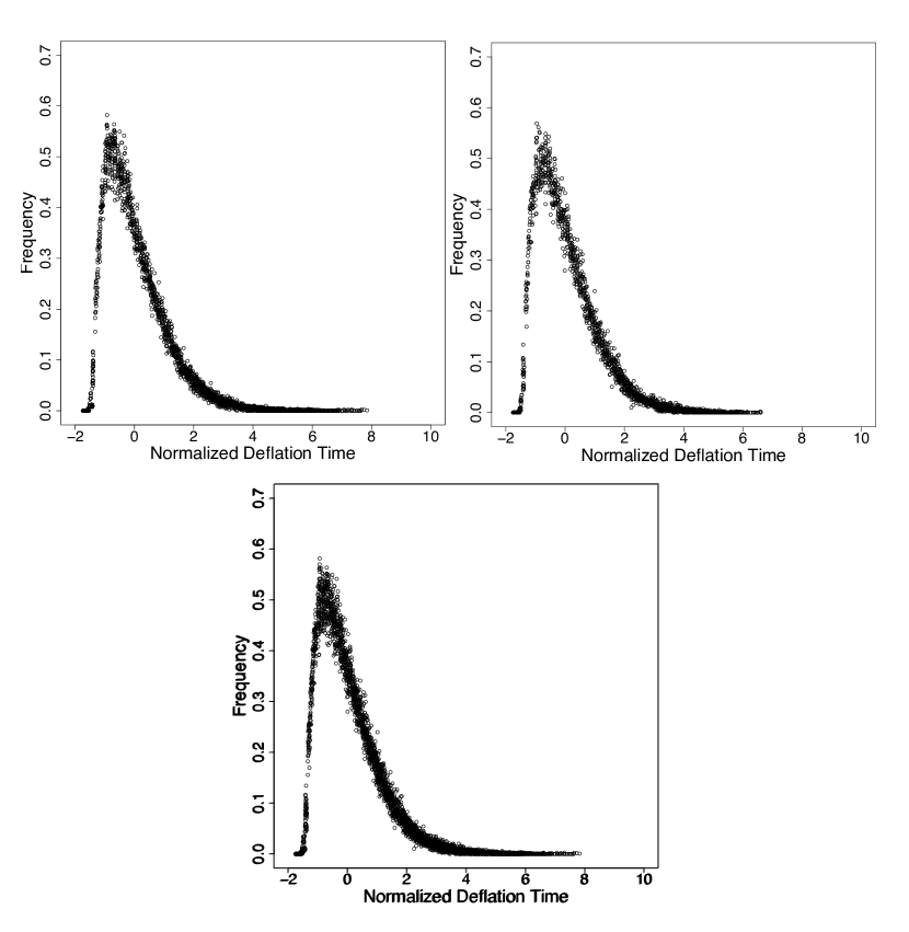
Figure 1: The observation of two-component universality for $\tau_{\epsilon,n,A,E}$ when $A=\operatorname{QR}$. This figure is taken from [2]. Overlayed histograms demonstrate the collapse of the histogram of $\tau_{\epsilon,n,A,E}$ to a single curve. See the Appendix for the definitions of our choices for $E$. In the top-left figure, $E=\operatorname{GOE}$, and 40 histograms for $\tau_{\epsilon,\epsilon,A,E}$, are plotted one on top of the other for $\epsilon=10^{-k}$, $k=2,\!4,\!6,\!8$ and $n=10,\!30,\ldots,\!190$. The histograms are created with $\approx 10,\!000$ samples. The top-right figure displays the same information as that in the top-left position, but now for $E=BE$. In the lower figure, all $40+40$ histograms are overlayed and universality is evident: the data appears to follow a universal law for the fluctuations.

From Figure 1, we see that eigenvalue computation with the QR algorithm exhibits two-component universality, i.e., the fluctuations $\tau_{\epsilon,n,A,E}$ obey a universal law for all ensembles $E$ under consideration. The same is true for all three algorithms considered in [2]: The laws are different, however, for different algorithms $A$.

In the current paper, the work in [2] has been extended in various ways as follows. All matrix ensembles are described in the Appendix.

1.1 The Jacobi Algorithm

In the first set of computations, the authors consider the eigenvalue problem for random matrices $M\in S_{n}$ using the Jacobi algorithm (see, e.g. [4]): for $M\in S_{n}$, choose $i<j$ such that $|M_{ij}|\geq\max_{1\leq i^{\prime}<j^{\prime}\leq n}|M_{i^{\prime}j^{\prime}}|$, and let $G^{(ij)}\equiv G^{(ij)}(\theta)$ be the corresponding Givens rotation matrix: $G^{(ij)}_{i^{\prime}j^{\prime}}=\delta_{i^{\prime}j^{\prime}}$, for $i^{\prime},j^{\prime}\neq i,j$, and

$$\left[\begin{array}[]{cc}G^{(ij)}_{ii}&G^{(ij)}_{ij}\\ G^{(ij)}_{ji}&G^{(ij)}_{jj}\end{array}\right]=\left[\begin{array}[]{cc}\cos(\theta)&\sin(\theta)\\ -\sin(\theta)&\cos(\theta)\end{array}\right],~{}~{}(G^{(ij)})^{T}G^{(ij)}=I.$$

Here $\theta=\theta(M)$ is chosen so that $((G^{(ij)})^{T}MG^{(ij)})_{ij}=0$ and then $\varphi_{\operatorname{Jacobi}}(M)\equiv(G^{(ij)})^{T}MG^{(ij)}$. Clearly, $M^{\prime}=\varphi_{\operatorname{Jacobi}}(M)\in S_{n}$ and $\operatorname{spec}(M^{\prime})=\operatorname{spec}(M)$ and again (see [4]), $M_{k}=\varphi^{(k)}_{\operatorname{Jacobi}}(M)\rightarrow\Lambda=\operatorname{diag}(\lambda_{1},\ldots,\lambda_{n})$. The Jacobi algorithm has a very different character from QR-Toda type algorithms which are intimately connected to completely integrable Hamiltonian systems (see [5] and the references therein) Deflation, which is a useful measure for eigenvalue computation times for QR/Toda type algorithms, is not useful for the Jacobi algorithm. In place of $T_{\epsilon,n,A,E}$, we record the halting time $k_{\epsilon,n,A,E}$: the number of iterations it takes for the Jacobi algorithm to reduce the Frobenius norm of the off-diagonal elements to be less than a given $\epsilon$. Histograms are produced for an appropriate analog of $\tau_{\epsilon,n,A,E}$:

$$\tau_{\epsilon,n,A,E}(M)=\frac{k_{\epsilon,n,A,E}(M)-\langle k_{\epsilon,n,A,E}\rangle}{\sigma_{\epsilon,n,A,E}}.$$ (2)

Computations for $A=\operatorname{Jacobi}$ are given in Figure 2. Again, two-component universality is evident.

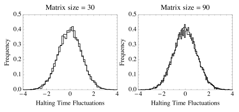
Figure 2: The observation of two-component universality for $\tau_{\epsilon,n,A,E}$ when $A=\operatorname{Jacobi}$, $E=\operatorname{GOE},~{}\mathrm{BE}$ and $\epsilon=\sqrt{n}\,10^{-10}$. The left figure displays two histograms, one on top of the other, one for $\operatorname{GOE}$ and one for $\mathrm{BE}$, when $n=30$. The right figure displays the same information for $n=90$. All histograms are produced with $16,\!000$ samples. We see two-component universality emerge for $n$ sufficiently large: the histograms follow a universal (independent of $E$) law.

1.2 Ensembles with Dependent Entries

In all the above cases, including the calculations for the Jacobi algorithm, the matrices $M$ are real and the entries $M_{ij}$ are independent, subject only to the symmetry requirement $M_{ij}=M_{ji}$. In the second set of computations in the present paper, the authors consider $n\times n$ Hermitian matrices $M=M^{*}$ taken from various unitary ensembles (see e.g [7]) with probability distributions proportional to $e^{-n\mathrm{tr}V(M)}dM$ where $V:\mathbb{R}\rightarrow\mathbb{R}$ grows sufficiently rapidly as $|x|\rightarrow\infty$, and $dM$ is Lebesgue measure on the algebraically independent entries $M_{ij}=\mathrm{Re}\,M_{ij}+\sqrt{-1}\,\mathrm{Im}\,M_{ij}$ of $M$. Unless $V(x)$ is proportional to $x^{2}$, the entries of $M$ for such ensembles are dependent, and it is a non-trivial matter to sample the matrices. A novel technique for sampling such unitary ensembles was introduced recently [8] by two of the authors, S.O. and T.T., together with N. R. Rao, taking advantage of the representation of the eigenvalues of $M$ as a determinantal point process whose kernel is given in terms of orthogonal polynomials (see also [9]). Using this sampling technique, the authors of the present paper have considered the QR algorithm for various unitary ensembles. Histograms for the halting (= deflation) time fluctuations $\tau_{\epsilon,n,A,E}$, $A=QR$, are given in Figure 3 and again two-component universality is evident.

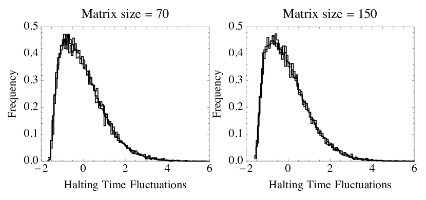
Figure 3: The observation of two-component universality for $\tau_{\epsilon,n,A,E}$ when $A=\operatorname{QR}$, $E=\mathrm{QUE},~{}\operatorname{COSH},~{}\mathrm{GUE}$ and $\epsilon=10^{-10}$. Here we are using deflation time ( = halting time), as in [2]. The left figure displays three histograms, one each for $\operatorname{GUE},~{}\operatorname{COSH}$ and $\operatorname{QUE}$, when $n=70$. The right figure displays the same information for $n=150$. All histograms are produced with $16,\!000$ samples. Two-component universality emerges for $n$ sufficiently large: the histograms follow a universal (independent of $E$) law. This is surprising because $\operatorname{COSH}$ and $\operatorname{QUE}$ have eigenvalue distributions that differ significantly from $\operatorname{GUE}$ in that they do not follow the so-called semi-circle law. These histograms appear to collapse to the same curve in Figure 1. This is a further surprise, given the well-known fact that Orthogonal and Unitary Ensembles give rise to different (eigenvalue) universality classes.

1.3 The Conjugate Gradient Algorithm

In a third set of computations in this paper, the authors start to address the question of whether two-component universality is just a feature of eigenvalue computation, or is present more generally in numerical computation. In particular, the authors consider the solution of the linear system of equations $Wx=b$ where $W$ is real and positive definite, using the conjugate gradient (CG) method. The method is iterative (see e.g. [10] and also Remark 1 below) and at iteration $k$ of the algorithm an approximate solution $x_{k}$ of $Wx=b$ is found and the residual $r_{k}=Wx_{k}-b$ is computed. For any given $\epsilon>0$, the method is halted when $\|r_{k}\|_{2}<\epsilon$, and the halting time $k_{\epsilon}(W,b)$ recorded. The authors consider $n\times n$ matrices $W$ chosen from two different positive definite ensembles $E$ (see Appendix A.3) and vectors $b=(b_{j})$ chosen independently with iid entries $\{b_{j}\}$. Given $\epsilon$ (small) and $n$ (large), and $(W,b)\in E$, the authors record the halting time $k_{\epsilon,n,A,E}$, $A=\operatorname{CG}$, and compute the fluctuations $\tau_{\epsilon,n,A,E}(W,b)$. The histograms for $\tau_{\epsilon,n,A,E}$ are given in Figure 4, and again, two-component universality is evident.

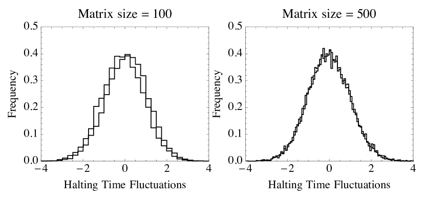
Figure 4: The observation of two-component universality for $\tau_{\epsilon,n,A,E}$ when $A=\operatorname{CG}$ and $E=\mathrm{cLOE},~{}\mathrm{cPBE}$ with $\epsilon=10^{-10}$. The left figure displays two histograms, one for $\mathrm{cLOE}$ and $\mathrm{cPBE}$, when $n=100$. The right figure displays the same information for $n=500$. All histograms are produced with $16,\!000$ samples. Two-component universality is evident for $n$ sufficiently large: the histograms follow a universal (independent of $E$) law. The critical scaling (see Appendix A.3) has significant impact on the distribution of the condition number and forces $\langle\tau_{\epsilon,n,A,E}\rangle\approx n\alpha$, $\alpha<1$. If the scaling $m=2n$ is chosen in the ensemble $E$ then the CG method converges too quickly and the halting time tends to take only 10-15 different values for each value of $m$. No interesting limiting statistics are present. Conversely, if $m=n$ the CG method converges slowly ($\langle k_{\epsilon,m,A,E}\rangle\gg m$) and rounding errors dominate the computation. Experiments do not indicate two-component universality if $m=2n$ or $m=n$. The scaling $m=n+2\lfloor\sqrt{n}\rfloor$ identifies a critical scaling region. Within this scaling region, we see two-component universality emerge for $n$ sufficiently large: the histograms follow a universal (independent of $E$) law.

1.4 The GMRES Algorithm

In a fourth set of computations, the authors again consider the solution of $Wx=b$ but here $W$ has the form $I+X$ and $X\equiv X_{n}$ is a random, real non-symmetric matrix and $b=(b_{j})$ is independent with uniform iid entries $\{b_{j}\}$. As $W=I+X$ is (almost surely) no longer positive definite the conjugate gradient algorithm breaks down, and the authors solve $(I+X)x=b$ using the Generalized Minimal Residual (GMRES) algorithm [11]. Again, the algorithm is iterative and at iteration $k$ of the algorithm an approximate solution $x_{k}$ of $(I+X)x=b$ is found and the residual $r_{k}=(I+X)x_{k}-b$ is computed. As before, for any given $\epsilon>0$, the method is halted when $\|r_{k}\|_{2}<\epsilon$ and $k_{\epsilon,n,A,E}(X,b)$ is recorded. As in the conjugate gradient problem (Section 1.3), the authors compute the histograms for the fluctuations of the halting time $\tau_{\epsilon,n,A,E}$ (2) for two ensembles $E$, where now $A=\operatorname{GMRES}$. The results are given in Figure 5, where again two-component universality is evident.

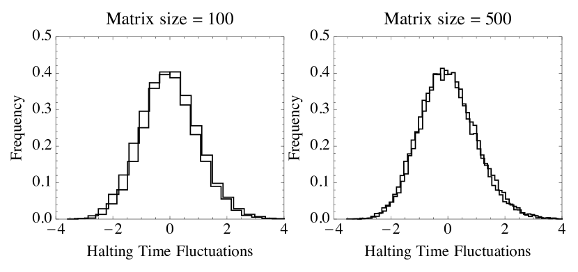
Figure 5: The observation of two-component universality for $\tau_{\epsilon,n,A,E}$ when $A=\operatorname{GMRES}$, $E=\mathrm{cSGE},~{}\mathrm{cSBE}$ and $\epsilon=10^{-8}$. The left figure displays two histograms, one for $\mathrm{cSGE}$ and one for $\mathrm{cSBE}$, when $n=100$. The right figure displays the same information for $n=500$. All histograms are produced with $16,\!000$ samples. The critically scaled ensembles cSBE and cSGE are of the form $I+X_{n}$ with $\|X_{n}\|\approx 2$. If the matrix is too close to the identity, the halting time will take almost constant values, i.e. $k_{\epsilon,n,A,E}=8$, independent of $n$. If the matrix is too far from the identity, the fact that it is unstructured makes GMRES perform poorly and the algorithm typically completes in $n$ steps, the maximum possible number of iterations (see Remark 1 below). With the proper scaling of $X$, we see two-component universality emerge for $n$ sufficiently large: the histograms follow a universal (independent of $E$) law.

Remark 1.

The computations in Sections 1.3 and 1.4 are particularly revealing for the following reason. Both the CG and GMRES algorithms proceed by generating approximations $x_{n}$ to the solution in progressively larger subspaces $V_{k}$ of $\mathbb{R}^{n}$, $x_{k}\in V_{k}$, $\dim V_{k}=k$ (almost surely). These algorithms terminate in at most $n$ steps, in the absence of rounding errors. If the matrix $W$ in the case of CG, or $I+X$ in the case of GMRES, is too close to the identity, then the algorithm will converge in $\mathcal{O}(1)$ steps, essentially independent of $n$. On the other hand, if $W$ or $I+X$ is too far from the identity, the algorithm will converge only after $n$ steps (GMRES) or be dominated by rounding errors (CG). Thus in both cases there are no meaningful statistics. What the calculations in Sections 1.3 and 1.4 reveal is that if the ensembles for CG and GMRES are such that the matrices $W$ and $I+X$, respectively, are typically not too close to, and not too far, from the identity, then the algorithms exhibit significant statistical fluctuations, and two-component universality is immediately evident. (for more discussion see the captions for Figures 4 and 5). Analogous considerations apply in Section 1.5 below.

1.5 Discretization of a Random PDE

In a fifth set of computations, the authors raise the issue of whether two-component universality is just a feature of finite-dimensional computation, or is also present in problems which are intrinsically infinite dimensional. In particular, is the universality present in numerical computations for PDEs? As a case study, the authors consider the numerical solution of the Dirichlet problem $\Delta u=0$ in a star-shaped region $\Omega\subset\mathbb{R}^{2}$ with $u=f$ on $\partial\Omega$. The boundary is described by a periodic function of the angle $\theta$, $r=r(\theta)$, and similarly $f=f(\theta)$, $0\leq\theta\leq 2\pi$. Two ensembles, BDE and UDE (as described in Appendix A.6), are derived from a discretization of the problem with specific choices for $r$, defined by a random Fourier series. The boundary condition $f$ is chosen randomly by letting $\{f(\frac{2\pi j}{n})\}_{j=0}^{n-1}$ be iid uniform on $[-1,1]$. Histograms for the halting time $\tau_{\epsilon,n,A,E}$ from these computations are given in Figure 6 and again, two-component universality is evident. What is surprising, and quite remarkable, about these computations is that the histograms for $\tau_{\epsilon,500,A,E}$ in this case are the same as the histograms for $\tau_{\epsilon,500,A,E}$ in Figure 5 (see Figure 6 for the overlayed histograms). In other words, UDE and BDE are structured with random components, whereas cSGE and cSBE have no structure, yet they produce the same statistics (modulo two components).

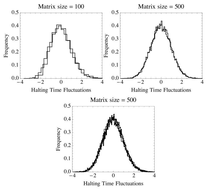
Figure 6: The observation of two-component universality for $\tau_{\epsilon,n,A,E}$ when $A=\operatorname{GMRES}$, $E=\mathrm{UDE},~{}\mathrm{BDE}$ and $\epsilon=10^{-8}$. The left figure displays two histograms, one for $\mathrm{UDE}$ and one for $\mathrm{BDE}$, when $n=100$. The right figure displays the same information for $n=500$. The bottom figure consists of four histograms, two taken from Figure 5 ($E=\mathrm{cSGE},~{}\mathrm{cSBE}$) and two taken from the right figure above ($E=\mathrm{UDE},~{}\mathrm{BDE}$). All histograms are produced with $16,\!000$ samples. It is interesting to note two properties. First, as we observe from our computations, BDE and UDE are of the form $I+X_{n}$ where $X_{n}$ has a norm that grows proportional to some fractional power of $n$. While this type of growth in the case of Section 1.4 (Figure 5) would cause GMRES to take its maximum possible number of iterations, that is $k=n$, nevertheless, in the context of Section 1.5, non-trivial statistics emerge. In light of Remark 1, we conjecture that structure is necessary for GMRES to perform well when the perturbation of the identity has an unbounded spectral radius in the large $n$ limit. The second, and most important feature, is that two-component universality for matrices of the form $I+X_{n}$ persists as the computations are moved from structured randomness (UDE and BDE) to unstructured randomness (cSBE and cSGE): the histograms follow a universal (independent of $E$) law.

1.6 A Genetic Algorithm

In all the computations discussed so far, the randomness in the computations resides in the initial data. In the sixth set of computations, the authors consider an algorithm which is intrinsically stochastic. They consider a genetic algorithm to compute Fekete points (see [12, p. 142]). Such points $P^{*}=(P_{1}^{*},P_{2}^{*},\ldots,P^{*}_{N})\in\mathbb{R}^{N}$ are the global minimizers of the objective function

$$H(P)=\frac{2}{N(N-1)}\sum_{1\leq i\neq j\leq N}\log|P_{i}-P_{j}|^{-1}+\frac{1}{N}\sum_{i=1}^{N}V(P_{i})$$

for real-valued functions $V=V(x)$ which grow sufficiently rapidly as $|x|\rightarrow\infty$. It is well-known (see, e.g. [12]) that as $N\rightarrow\infty$, the counting measures $\delta_{P^{*}}=\frac{1}{N}\sum_{i=1}^{N}\delta_{P_{i}^{*}}$ converge to the so-called equilibrium measure $\mu_{V}$ which plays a key role in the asymptotic theory of the orthogonal polynomials generated by measure $e^{-NV(x)}dx$ on $\mathbb{R}$. Genetic algorithms involve two basic components , “mutation” and “crossover”. The authors implement the genetic algorithm in the following way.

The Algorithm

Fix a distribution $\mathfrak{D}$ on $\mathbb{R}$. Draw an initial population $\mathcal{P}_{0}=\mathcal{P}=\{P_{i}\}_{i=1}^{n}$ consisting of $n=100$ vectors in $\mathbb{R}^{N}$, $N$ large, with elements that are iid uniform on $[-4,4]$. The random map $F_{\mathfrak{D}}(\mathcal{P}):(\mathbb{R}^{N})^{n}\rightarrow(\mathbb{R}^{N})^{n}$ is defined by one of the following two procedures:

• Mutation: Pick one individual $P\in\mathcal{P}$ at random (uniformly). Then pick two integers $n_{1},~{}n_{2}$ from $\{1,2,\ldots,N\}$ at random (uniformly and independent). Three new individuals are created.

  • $\tilde{P}_{1}$ — draw $n_{1}$ iid numbers $\{x_{1},\ldots,x_{n_{1}}\}$ from $\mathfrak{D}$ and perturb the first $n_{1}$ elements of $P$ : $(\tilde{P}_{1})_{i}=(P)_{i}+x_{i}$, $i=1,\ldots,n_{1}$, and $(\tilde{P}_{1})_{i}=(P)_{i}$ for $i>n_{1}$.

  • $\tilde{P}_{2}$ — draw $N-n_{2}$ iid numbers $\{y_{n_{2}+1},\ldots,y_{N}\}$ from $\mathfrak{D}$ and perturb the last $N-n_{2}$ elements of $P$: $(\tilde{P}_{2})_{i}=(P)_{i}+y_{i}$, $i=n_{2}+1,\ldots,N$, and $(\tilde{P}_{2})_{i}=(P)_{i}$ for $i\leq n_{2}$.

  • $\tilde{P}_{3}$ — draw $|n_{1}-n_{2}|$ iid numbers $\{z_{1},\ldots,z_{|n_{1}-n_{2}|}\}$ from $\mathfrak{D}$ and perturb elements $n_{1}^{*}=1+\min(n_{1},n_{2})$ through $n_{2}^{*}=\max(n_{1},n_{2})$: $(\tilde{P}_{3})_{i}=(P)_{i}+z_{i-n_{1}^{*}+1}$, $i=n_{1}^{*},\ldots,n_{2}^{*}$, and $(\tilde{P}_{3})_{i}=(P)_{i}$ for $i\not\in\{n_{1}^{*},\ldots,n_{2}^{*}\}$.

• Crossover: Pick two individuals $P,~{}Q$ from $\mathcal{P}$ at random (independent and uniformly). Then pick two numbers $n_{1},~{}n_{2}$ from $\{1,2,\ldots,N\}$ (independent and uniformly). Two new individuals are created.

  • $\tilde{P}_{4}$ — Replace the $n_{1}$th element of $P$ with the $n_{2}$th element of $Q$ and perturb it (additively) with a sample of $\mathfrak{D}$.

  • $\tilde{P}_{5}$ — Replace the $n_{1}$th element of $Q$ with the $n_{2}$th element of $P$ and perturb it (additively) with a sample of $\mathfrak{D}$.

At each step, the application of either crossover or mutation is chosen with equal probability. The new individuals are appended to $\mathcal{P}$ and $\mathcal{P}\mapsto\mathcal{P}^{\prime}=F_{\mathfrak{D}}(\mathcal{P})\in(\mathbb{R}^{N})^{n}$ is constructed by choosing the 100 $P_{i}$’s in $\tilde{\mathcal{P}}$ which yield the smallest values of $H(P)$. The algorithm produces a sequence of populations $\mathcal{P}_{1},\mathcal{P}_{2},\ldots,\mathcal{P}_{k},\ldots$ in $(\mathbb{R}^{N})^{n}$, $\mathcal{P}_{k+1}=F_{\mathfrak{D}}(\mathcal{P})$, $n=100$, and halts, with halting time recorded, for a given $\epsilon$, when $\min_{P\in\mathcal{P}_{k}}H(P)-\inf_{P\in\mathbb{R}^{N}}H(P)<\epsilon$.

The histograms for the fluctuations $\tau_{\epsilon,N,A,E}$, with $A=\operatorname{Genetic}$ are given in Figure 7, for two choices of $V$, $V(x)=x^{2}$ and $V(x)=x^{4}-3x^{2}$, and different choices of $E\simeq\mathfrak{D}$. For $V(x)=x^{2}$ $\inf_{P\in\mathbb{R}^{N}}H(P)$ is known explicitly, and for $V(x)=x^{4}-3x^{2}$, $\inf_{P\in\mathbb{R}^{N}}H(P)$ is approximated by a long run of the genetic algorithm. As before, two-component universality is evident.

Figure 7: The observation of two-component universality for $\tau_{\epsilon,N,A,E}$ when $A=\operatorname{Genetic}$, $\epsilon=10^{-2}$ and $E\simeq\mathfrak{D}$ where $\mathfrak{D}$ is chosen to be either uniform on $[-1/(10N),1/(10N)]$ or taking values $\pm 1/(10N)$ with equal probability. The top row is created with the choice $V(x)=x^{2}$ and the bottom row with $V(x)=x^{4}-3x^{2}$. Each of the plots in the left column displays two histograms, one for each choice of $\mathfrak{D}$ when $N=10$. The right column displays the same information for $N=40$. All histograms are produced with $16,\!000$ samples. It is evident that the histograms collapse onto a universal curve, one for each $V$.

1.7 Curie–Weiss Model

In the seventh and final set of computations, the authors pick up on a common notion in neuroscience that the human brain is a computer with software and hardware. If this is indeed so, then one may speculate that two-component universality should certainly be present in some cognitive actions. Indeed, such a phenomenon is in evidence in the recent experiments of Bakhtin and Correll [13]. In [13], data from experiments with 45 human participants was analyzed. The participants are shown 200 pairs of images. The images in each pair consist of nine black disks of variable size. The disks in the images within each pair have approximately the same area so that there is no a priori bias. The participants are then asked to decide which of the two images covers a larger (black) area and the time $T$ required to make a decision is recorded. For each participant, the decision times for the 200 pairs are collected and the fluctuation histogram is tabulated. The experimental results are in good agreement with a dynamical Curie-Weiss model frequently used in describing decision processes [14]. As each of the 45 participants operates, presumably, in his’r own stochastic neural environment, this is a remarkable demonstration of two-component universality in cognitive action.

At its essence the Curie–Weiss model is Glauber dynamics on the hypercube $\{-1,1\}^{N}$ with a microscopic approximation of a drift-diffusion process. Consider $N$ variables $\{X_{i}(t)\}_{i=1}^{N}$, $X_{i}(t)\in\{-1,1\}$. The state of the system at time $t$ is $X(t)=(X_{1}(t),X_{2}(t),\ldots,X_{N}(t))$. The transition probabilities are given through the expressions

$$\mathbb{P}(X_{i}(t+\Delta t)\neq X_{i}(t)|X(t)=x)=c_{i}(x)\Delta t+o(\Delta t),$$

where $c_{i}(x)$ is the spin flip intensity. The observable considered is $M(X(t))=\frac{1}{N}\sum_{i=1}^{N}X_{i}(t)\in[-1,1]$, and the initial state of the system is chosen so that $M(X(0))=0$, a state with no a priori bias, as in the case of the experimental setup. The halting (or decision) time for this model is $k=\inf\{t:|M(X(t))|\geq\epsilon\}$, the time at which the system makes a decision. Here $\epsilon\in(0,1)$ may not be small.

This model is simulated by first sampling an exponential random variable with mean $\lambda(t)=\left(\sum_{i}c_{i}(X(t))\right)^{-1}$ to find the time $\Delta t$ at which the system changes state. Sampling the random variable $Y$, $\mathbb{P}(Y=i)=c_{i}(X(t))\lambda(t)$, $i=1,2,\ldots,N$ produces an integer $j$, determining which spin flipped. Define $X_{i}(t+s)\equiv X_{i}(t)$ if $s\in[0,\Delta t)$ for $i=1,2,\ldots,N$ and $X_{i}(t+\Delta t)\equiv X_{i}(t)$, $X_{j}(t+\Delta t)\equiv-X_{j}(t)$ for $i\neq j$. This procedure is repeated with $t$ replaced by $t+\Delta t$ to evolve the system.

Central to the application of the model is the assumption on the statistics of the spin flip intensity $c_{i}(x)$. If one changes the basic statistics of the $c_{i}$’s, will the limiting histograms for the fluctuations of $k$ be affected as $N$ becomes large? In response to this question the authors consider the following choices for $E\simeq c_{i}(x)$ ($\beta=1.3$): $c_{i}(x)=o_{i}(x)=e^{-\beta x_{i}M(x)}$ (the case studied in [13]), $c_{i}(x)=u_{i}(x)=e^{-\beta x_{i}(M(x)-M^{3}(x)/5)}$, or $c_{i}(x)=v_{i}(x)=e^{-\beta x_{i}(M(x)+M^{8}(x))}$. The resulting histograms for the fluctuations $\tau_{\epsilon,N,A,E}$ of $T$ are given in Figure 8. Once again, two-component universality is evident. Thus the universality in the decision process models mirrors the universality observed among the 45 participants in the experiment of Bakhtin and Correll.

Figure 8: The observation of two-component universality for $\tau_{\epsilon,N,A,E}$ when $A=\text{Curie--Weiss}$, $E\simeq o_{i},~{}u_{i},~{}v_{i}$, $\epsilon=.5$ and $\beta=1.3$. The left figure displays three histograms, one for each choice of $E$ when $N=50$. The right figure displays the same information for $N=200$. All histograms are produced with $16,\!000$ samples. The histogram for $E=o_{i}$ corresponds to the case studied in [13, 14]. It is clear from these computations that the fluctuations collapse on to the universal curve for $E=o_{i}$. Thus, reasonable changes in the spin flip intensity do not appear to change the limiting histogram. This indicates why the specific choice made in [13] of $E=o_{i}$ is perhaps enough to capture the behavior of many individuals.

2 Conclusions

Two distinct themes are combined in this work: (1) the notion of universality in random matrix theory and statistical physics; (2) the use of random ensembles in scientific computing. The origin of both these ideas dates to the 1950s in the work of (1) Wigner [7, 15], and (2) von Neumann and Goldstine [16]. There has been considerable progress in the rigorous understanding of universality in random matrix theory (see e.g. [17, 18] and the references therein). In contrast, the performance of numerical algorithms on random ensembles is less understood, though results in this area include probabilistic bounds for condition numbers and halting times for numerical algorithms [19, 20, 21].

The work presented here reveals empirical evidence for two-component universality in several numerical algorithms. The results of [2] and Sections 1.1-1.5 reveal universal fluctuations of halting times for iterative algorithms in numerical linear algebra on random matrix ensembles with both dependent and independent entries. In each instance, the process of numerical computation on a random matrix may be viewed as the evolution of a random ensemble by a deterministic dynamical system. In a similar light, the algorithms of Section 1.6 and 1.7 may be seen as stochastic dynamical systems with that in Section 1.7 having a close connection with neural computation. In all these examples, the empirical observations presented here suggest new universal phenomena in non-equilibrium statistical mechanics. The results of Section 1.4 and 1.5 reveal that numerical computations with a structured ensemble with some random components may have the same statistics (modulo two-components) as an unstructured ensemble. This brings to mind the situation in the 1950s when Wigner introduced random matrices as a model for scattering resonances of neutrons off heavy nuclei: the neutron-nucleus system has a well-defined and structured Hamiltonian, but nevertheless the resonances for neutron scattering are well-described statistically by the eigenvalues of an (unstructured) random matrix.

Materials

All algorithms discussed here are implemented in Mathematica. A package is available for download [1] that contains all relevant data and the code to generate this data. The package supports parallel evaluation for most algorithms and runs easily on personal computers.

A.1 Gaussian Ensembles

The Gaussian Orthogonal Ensemble (GOE) is given by $(X+X^{T})/\sqrt{4n}$ where $X$ is an $n\times n$ matrix of standard iid Gaussian variables. The Gaussian Unitary Ensemble (GUE) is given by $(X+X^{*})/\sqrt{8n}$ where $X$ is an $n\times n$ matrix of standard iid complex Gaussian variables.

A.2 Bernoulli Ensemble

The Bernoulli Ensemble (BE) is given by an $n\times n$ matrix $X$ consisting of iid random variables that take the values $\pm 1/\sqrt{n}$ with equal probability subject only to the constraint $X^{T}=X$.

A.3 Positive Definite Ensembles

The critically-scaled Laguerre Orthogonal Ensemble (cLOE) is given by $W=XX^{T}/m$ where $X$ is an $n\times m$ matrix with standard iid Gaussian entries. The critically-scaled positive definite Bernoulli ensemble (cPBE) is given by $W=XX^{T}/m$ where $X$ is an $n\times m$ matrix consisting of iid Bernoulli variables taking the values $\pm 1$ with equal probability. In both cases, the critical scaling refers to the choice $m=n+2\lfloor\sqrt{n}\rfloor$.

A.4 Shifted Ensembles

The critically-scaled shifted Bernoulli Ensemble (cSBE) is given by $I+X/\sqrt{n}$ where $X$ is an $n\times n$ matrix consisting of iid Bernoulli variables taking the values $\pm 1$ with equal probability. The critically-scaled shifted Ginibre Ensemble (cSGE) is given by $I+X/\sqrt{n}$ where $X$ is an $n\times n$ matrix of standard iid Gaussian variables. With this scaling $\mathbb{P}(|\|X/\sqrt{n}\|-2|>\epsilon)\rightarrow 0$ as $n\rightarrow\infty$ [22].

A.5 Unitary Ensembles

The Quartic Unitary Ensemble (QUE) is a complex, unitary ensemble with probability distribution proportional to $e^{-n\mathrm{tr}M^{4}}dM$. The Cosh Unitary Ensemble (COSH) has its distribution proportional to $e^{-\mathrm{tr}\cosh M}dM$.

A.6 Dirichlet Ensembles

We consider the numerical solution of the equation $\Delta u=0$ in $\Omega$ and $u=f$ on $\partial\Omega$. Here we let $\Omega$ be the star-shaped region interior to the curve $(x,y)=(r(\theta)\cos(\theta),r(\theta)\sin(\theta))$ where $r(\theta)$ for $0\leq\theta<2\pi$ is given by $r(\theta)=1+\sum_{j=1}^{m}(X_{j}\cos(j\theta)+Y_{j}\sin(j\theta)),$ and $X_{j}$ and $Y_{j}$ are iid random variables on $[-1/(2m),1/(2m)]$. The boundary integral equation

$$\pi u(P)-\int_{\partial\Omega}u(P)\frac{\partial}{\partial n_{Q}}\log|P-Q|dS_{Q}=-f(P),\quad P\in\partial\Omega,$$

is solved by discretizing in $\theta$ with $n$ points and applying the trapezoidal rule with $n=2m$ (see [23]). For the Bernoulli Dirichlet Ensemble (BDE), $X_{m}$ and $Y_{m}$ are Bernoulli variables taking values $\pm 1/(2m)$ with equal probability. For the Uniform Dirichlet Ensemble (UDE), $X_{m}$ and $Y_{m}$ are uniform variables on $[-1/(2m),1/(2m)]$.

References

-
[1]
Trogdon T
(2014) Numerical Universality:
https://bitbucket.org/trogdon/numericaluniversality. - [2] Pfrang C, Deift P, Menon G (2012) How long does it take to compute the eigenvalues of a random symmetric matrix? arXiv Prepr. arXiv1203.4635.
- [3] Parlett BN (1998) The Symmetric Eigenvalue Problem (SIAM, Philadelphia, PA), p 398.
- [4] Golub GH, Loan CFV (2013) Matrix Computations (JHU Press, Baltimore, MD), p 756.
- [5] Deift P, Nanda T, Tomei C (1983) Ordinary differential equations and the symmetric eigenvalue problem. SIAM J. Numer. Anal. 20:1–22.
- [6] Demmel J, Veselić K (1992) Jacobi’s method is nore accurate than QR. SIAM J. Matrix Anal. Appl. 13:1204–1245.
- [7] Mehta ML (2004) Random Matrices (Academic Press, New York, NY), p 688.
- [8] Olver S, Rao NR, Trogdon T (2014) Sampling unitary invariant ensembles. arXiv Prepr. arXiv1404.0071.
- [9] Li XH, Menon G (2013) Numerical solution of Dyson Brownian motion and a sampling scheme for invariant matrix ensembles. J. Stat. Phys. 153:801–812.
- [10] Saad Y (2003) Iterative methods for sparse linear systems (SIAM, Philadelphia, PA), p 528.
- [11] Saad Y, Schultz MH (1986) GMRES: a generalized minimal residual algorithm for solving nonsymmetric linear systems. SIAM J. Sci. Stat. Comput. 7:856–869.
- [12] Saff EB, Totik V (1997) Logarithmic Potentials with External Fields (Springer, New York, NY), p 509.
- [13] Bakhtin Y, Correll J (2012) A neural computation model for decision-making times. J. Math. Psychol. 56:333–340.
- [14] Bakhtin Y (2011) Decision making times in mean-field dynamic Ising model. Ann. Henri Poincaré 13:1291–1303.
- [15] Wigner EP (1951) On the statistical distribution of the widths and spacings of nuclear resonance levels. Math. Proc. Cambridge Philos. Soc. 47:790–798.
- [16] Goldstine HH, von Neumann J (1951) Numerical inverting of matrices of high order. II. Proc. AMS 2:188–202.
- [17] Deift P, Gioev D (2009) Random matrix theory: invariant ensembles and universality, Courant Lecture Notes in Mathematics (Amer. Math. Soc., Providence, RI) Vol. 18, p 217.
- [18] Erdős L, Yau H (2012) Universality of local spectral statistics of random matrices. Bull. Am. Math. Soc. 49:377–414.
- [19] Demmel J (1988) The probability that a numerical analysis problem is difficult. Math. Comput. 50:449–480.
- [20] Edelman A (1988) Eigenvalues and condition numbers of random matrices. SIAM J. Matrix Anal. Appl. 9:543–560.
- [21] Smale S (1985) On the efficiency of algorithms of analysis. Bull. Am. Math. Soc. 13:87–121.
- [22] Geman S (1980) A limit theorem for the norm of random matrices. Ann. Probab. 8:252–261.
- [23] Atkinson K, Han W (2009) Theoretical Numerical Analysis (Springer, New York, NY).