Poincaré Series for Tensor Invariants and the McKay Correspondence

Abstract

For a finite group $\mathsf{G}$ and a finite-dimensional $\mathsf{G}$-module $\mathsf{V}$, we prove a general result on the Poincaré series for the $\mathsf{G}$-invariants in the tensor algebra $\mathsf{T}(\mathsf{V})=\bigoplus_{k\geq 0}\mathsf{V}^{\otimes k}$. We apply this result to the finite subgroups $\mathsf{G}$ of the $2\times 2$ special unitary matrices and their natural module $\mathsf{V}$ of $2\times 1$ column vectors. Because these subgroups are in one-to-one correspondence with the simply laced affine Dynkin diagrams by the McKay correspondence, the Poincaré series obtained are the generating functions for the number of walks on the simply laced affine Dynkin diagrams.

MSC Numbers (2010): 14E16, 05E10, 20C05
Keywords: tensor invariants, Poincaré series, McKay correspondence, Schur-Weyl duality

1 Introduction

Let $\mathsf{G}$ be a group, and assume $\{\mathsf{G}^{\lambda}\mid\lambda\in\Lambda(\mathsf{G})\}$ is the set of finite-dimensional irreducible $\mathsf{G}$-modules over the complex field $\mathbb{C}$. Associated to a fixed finite-dimensional $\mathsf{G}$-module $\mathsf{V}$ over $\mathbb{C}$ is the representation graph $\mathcal{R}_{\mathsf{V}}(\mathsf{G})$ having nodes indexed by the $\lambda$ in $\Lambda(\mathsf{G})$ and $a_{\mu,\lambda}$ edges from $\mu$ to $\lambda$ in $\mathcal{R}_{\mathsf{V}}(\mathsf{G})$ if

$$\mathsf{G}^{\mu}\otimes\mathsf{V}=\bigoplus_{\lambda\in\Lambda(\mathsf{G})}a_{\mu,\lambda}\mathsf{G}^{\lambda}.$$ (1.1)

Thus, the number of edges $a_{\mu,\lambda}$ from $\mu$ to $\lambda$ in $\mathcal{R}_{\mathsf{V}}(\mathsf{G})$ is the multiplicity of $\mathsf{G}^{\lambda}$ as a summand of $\mathsf{G}^{\mu}\otimes\mathsf{V}$.

When $\mathsf{G}$ is a finite group, the representation graph and the characters of $\mathsf{G}$ are closely related. Assume $\chi_{\mathsf{V}}$ is the character of $\mathsf{V}$, and $\chi_{\lambda}$ is the character of $\mathsf{G}^{\lambda}$ for $\lambda\in\Lambda(\mathsf{G})$. Let $\mathsf{d}=\,\mathsf{dim}\,\mathsf{V}=\chi_{\mathsf{V}}(1)$. Steinberg [Ste] has shown that when the action of $\mathsf{G}$ on $\mathsf{V}$ is faithful, the following hold:

• The eigenvalues of the matrix $\big{(}\mathsf{d}\,\delta_{\mu,\lambda}-a_{\mu,\lambda}\big{)}$ are $\mathsf{d}-\chi_{\mathsf{V}}(g)$ as $g$ ranges over a set $\Gamma$ of conjugacy class representatives of $\mathsf{G}$.

• The column vector $\big{(}\chi_{\lambda}(g)\big{)}$ with entries given by the character values of the irreducible $\mathsf{G}$-modules at $g$ is an eigenvector corresponding to $\mathsf{d}-\chi_{\mathsf{V}}(g)$. These vectors form the columns of the character table of $\mathsf{G}$.

• The vector $\big{(}\mathsf{d}^{\lambda}\big{)}$, whose entries are the dimensions $\mathsf{d}^{\lambda}=\,\mathsf{dim}\,\mathsf{G}^{\lambda}=\chi_{\lambda}(1)$ of the irreducible $\mathsf{G}$-modules, corresponds to the eigenvalue 0.

Let $\mathsf{G}^{0}$ be the one-dimensional trivial $\mathsf{G}$-module on which every element of the group acts as the identity transformation, and let $\mathsf{m}_{k}^{\lambda}$ be the number of walks of $k$ steps from $0$ to $\lambda$ on the representation graph $\mathcal{R}_{\mathsf{V}}(\mathsf{G})$. Since each step on the graph is accomplished by tensoring with $\mathsf{V}$, $\mathsf{m}_{k}^{\lambda}$ is the multiplicity of the irreducible $\mathsf{G}$-module $\mathsf{G}^{\lambda}$ in $\mathsf{G}^{0}\otimes\mathsf{V}^{\otimes k}\cong\mathsf{V}^{\otimes k}$.

In what follows, we identify $\mathsf{V}^{\otimes 0}\cong\mathbb{C}$ as a $\mathsf{G}$-module with $\mathsf{G}^{0}$, so that $\mathsf{m}_{0}^{\lambda}=\delta_{\lambda,0}$ (the Kronecker delta). For $\lambda\in\Lambda(\mathsf{G})$, we consider the Poincaré series

$$\mathsf{m}^{\lambda}(t)=\sum_{k\geq 0}\mathsf{m}_{k}^{\lambda}\,t^{k}$$ (1.2)

for the multiplicity of $\mathsf{G}^{\lambda}$ in the tensor algebra $\mathsf{T}(\mathsf{V})=\bigoplus_{k\geq 0}\mathsf{V}^{\otimes k}$, (which is also the generating function for the number of walks from 0 to $\lambda$ in $\mathcal{R}_{\mathsf{V}}(\mathsf{G})$). In particular, $\mathsf{m}^{0}(t)$ is the Poincaré series for the $\mathsf{G}$-invariants, $\mathsf{T}(\mathsf{V})^{\mathsf{G}}=\{w\in\mathsf{T}(\mathsf{V})\mid gw=w\ \hbox{for all}\ g\in\mathsf{G}\}$, in $\mathsf{T}(\mathsf{V})$.

The centralizer algebra,

$$\mathsf{Z}_{k}(\mathsf{G})=\{X\in\mathsf{End}(\mathsf{V}^{\otimes k})\mid Xgw=gXw\ \ \hbox{\rm for all}\ \ w\in\mathsf{V}^{\otimes k}\},$$

plays an essential role in understanding the $\mathsf{G}$-module $\mathsf{V}^{\otimes k}$. The idempotents that project $\mathsf{V}^{\otimes k}$ onto its irreducible $\mathsf{G}$-summands live in the finite-dimensional semisimple associative algebra $\mathsf{Z}_{k}(\mathsf{G})$. Schur-Weyl duality relates the decomposition of  $\mathsf{V}^{\otimes k}$ as a $\mathsf{G}$-module to the decomposition of  $\mathsf{V}^{\otimes k}$ as a $\mathsf{Z}_{k}(\mathsf{G})$-module revealing the following connections between the representation theories of $\mathsf{G}$ and $\mathsf{Z}_{k}(\mathsf{G})$:

• The irreducible $\mathsf{Z}_{k}(\mathsf{G})$-modules $\mathsf{Z}_{k}^{\lambda}$ are in bijection with the elements $\lambda$ of $\Lambda_{k}(\mathsf{G}):=\{\mu\in\Lambda(\mathsf{G})\mid\mathsf{m}_{k}^{\mu}\geq 1\}$.

• $\mathsf{V}^{\otimes k}\,\cong\,\displaystyle{\bigoplus_{\lambda\in\Lambda_{k}(\mathsf{G})}\mathsf{m}_{k}^{\lambda}\,\,\mathsf{G}^{\lambda}\quad\hbox{\rm and}\quad\mathsf{V}^{\otimes k}\,\cong\,\bigoplus_{\lambda\in\Lambda_{k}(\mathsf{G})}\mathsf{d}^{\lambda}\,\,\mathsf{Z}_{k}^{\lambda}}$.

• $\,\mathsf{dim}\,\mathsf{Z}_{k}^{\lambda}=\mathsf{m}_{k}^{\lambda}=$   number of walks of  $k$  steps from   0  to $\lambda$ on ${\mathcal{R}}_{\mathsf{V}}(\mathsf{G})$.

• $\,\mathsf{dim}\,\mathsf{G}^{\lambda}=\mathsf{d}^{\lambda}$.

• $\,\mathsf{dim}\,\,\mathsf{Z}_{k}(\mathsf{G})=\displaystyle{\sum_{\lambda\in\Lambda_{k}(\mathsf{G})}(\,\mathsf{dim}\,\,\mathsf{Z}_{k}^{\lambda})^{2}=\sum_{\lambda\in\Lambda_{k}(\mathsf{G})}(\mathsf{m}_{k}^{\lambda})^{2}}$.

• When the dual module $\mathsf{V}^{*}$ is isomorphic to $\mathsf{V}$ as a $\mathsf{G}$-module, then

  $\,\mathsf{dim}\,\,\mathsf{Z}_{k}(\mathsf{G})=$  number of walks of  $2k$  steps from   $0$   to  $0$   on   ${\mathcal{R}}_{\mathsf{V}}(\mathsf{G})$

  $=\,\mathsf{dim}\,\mathsf{Z}_{2k}^{0}$.

• As a $(\mathsf{G},\mathsf{Z}_{k}(\mathsf{G}))$-bimodule, $\mathsf{V}^{\otimes k}$ has a multiplicity-free decomposition,

  $\mathsf{V}^{\otimes k}\cong\displaystyle{\bigoplus_{\lambda\in\Lambda_{k}(\mathsf{G})}}\left(\mathsf{G}^{\lambda}\otimes\mathsf{Z}_{k}^{\lambda}\right)$.

• $\mathsf{m}^{\lambda}(t)=\sum_{k\geq 0}\mathsf{m}_{k}^{\lambda}\,t^{k}=\sum_{k\geq 0}\left(\,\mathsf{dim}\,\mathsf{Z}_{k}^{\lambda}\right)\,t^{k}.$

Often one is able to build the entire family of finite-dimensional irreducible $\mathsf{G}$-modules from a single well-chosen module $\mathsf{V}$ and its tensor powers by applying idempotents in the algebras $\mathsf{Z}_{k}(\mathsf{G})$ to project onto the irreducible $\mathsf{G}$-summands. Schur’s groundbreaking 1901 doctoral thesis constructed the finite-dimensional irreducible polynomial representations for the general linear group $\mathsf{GL}_{n}(\mathbb{C})$ from tensor powers of its defining module $\mathsf{V}=\mathbb{C}^{n}$ in exactly this way. The algebra $\mathsf{Z}_{k}(\mathsf{GL}_{n}(\mathbb{C}))$ is a homomorphic image of the group algebra $\mathbb{C}\mathbf{S}_{k}$ of the symmetric group $\mathbf{S}_{k}$ for $k\geq 1$, which acts by permuting the factors of $\mathsf{V}^{\otimes k}$.

Our aim here is to establish a general result about the Poincaré series $\mathsf{m}^{\lambda}(t)$ for arbitrary finite groups and then to apply this result to the finite subgroups $\mathsf{G}$ of the special unitary group

$${\mathsf{SU}_{2}}=\displaystyle{\left\{\begin{pmatrix}\ x&y\\ -\bar{y}&\bar{x}\end{pmatrix}\,\bigg{|}\ x,y\in\mathbb{C},\ \,x\bar{x}+y\bar{y}=1\right\}},$$

where “$\mkern 1.2mu\overline{\mkern-1.0mu\ \ \mkern-1.0mu}\mkern 1.0mu$” denotes complex conjugate. These subgroups are especially interesting because of the McKay correspondence and the vast literature it has inspired during the last 35 years.

In 1980, J. McKay [Mc1, Mc2] discovered a remarkable one-to-one correspondence between the isomorphism classes of the finite subgroups of $\mathsf{SU}_{2}$ and the simply laced affine Dynkin diagrams. Almost a century earlier, F. Klein had determined that a finite subgroup of $\mathsf{SU}_{2}$ must be isomorphic to one of the following: (a) a cyclic group $\mathbf{C}_{n}$ of order $n$, (b) a binary dihedral group $\mathbf{D}_{n}$ of order $4n$, or (c) one of the 3 exceptional groups: the binary tetrahedral group $\mathbf{T}$ of order 24, the binary octahedral group $\mathbf{O}$ of order 48, or the binary icosahedral group $\mathbf{I}$ of order 120. Binary here refers to the fact that the center is $\{\pm\mathrm{I}\}$, where $\mathrm{I}$ is the $2\times 2$ identity matrix, and the group modulo its center is a dihedral group or the rotational symmetry group of a tetrahedron, octahedron, or icosahedron in the exceptional cases.

The natural module for ${\mathsf{SU}_{2}}$ is the space $\mathsf{V}=\mathbb{C}^{2}=\left\{\big{(}\begin{smallmatrix}\cdot\\ \cdot\end{smallmatrix}\big{)}\right\}$ of $2\times 1$ column vectors, which ${\mathsf{SU}_{2}}$ and its finite subgroups $\mathsf{G}$ act on by matrix multiplication. McKay’s observation was that the representation graph $\mathcal{R}_{\mathsf{V}}(\mathsf{G})$ for $\mathsf{G}=\mathbf{C}_{n},\mathbf{D}_{n},\mathbf{T},\mathbf{O},\mathbf{I}$ is exactly the affine Dynkin diagram $\mathsf{\widehat{A}_{n-1}}$, $\mathsf{\widehat{D}_{n+2}}$, $\mathsf{\widehat{E}_{6}}$, $\mathsf{\widehat{E}_{7}}$, $\mathsf{\widehat{E}_{8}}$, respectively, with the vertex 0 being the affine node. Thus, the correspondence gives the pairings below. The label inside the node is the index of the irreducible $\mathsf{G}$-module, and the label above the node is its dimension, which is the mark on the Dynkin diagram. The trivial module is indicated in white and the module $\mathsf{V}=\mathbb{C}^{2}$ in black. In the cyclic case $\mathsf{V}=\mathbf{C}_{n}^{(n-1)}\oplus\mathbf{C}_{n}^{(1)}$, and in all other cases $\mathsf{V}=\mathsf{G}^{(1)}$.

$$\begin{array}[]{c}(\mathbf{C}_{n},\widehat{\mathsf{A}}_{n-1})\hskip 136.5733pt(\mathbf{D}_{n},\widehat{\mathsf{D}}_{n+2})\\ \includegraphics[scale={.65},page=3]{poincare-diagrams.pdf}\end{array}$$ (1.3)

$$\begin{array}[]{c}(\mathbf{T},\widehat{\mathsf{E}}_{6})\hskip 142.26378pt(\mathbf{O},\widehat{\mathsf{E}}_{7})\\ \includegraphics[scale={.6},page=4]{poincare-diagrams.pdf}\\ (\mathbf{I},\widehat{\mathsf{E}}_{8})\\ \includegraphics[scale={.6},page=5]{poincare-diagrams.pdf}\end{array}$$

Furthermore, the following hold:

• The sum $h:=\sum_{\lambda\in\Lambda(\mathsf{G})}\,\mathsf{dim}\,\mathsf{G}^{\lambda}$ of the dimensions (marks) is the Coxeter number of the corresponding finite Dynkin diagram obtained by deleting the affine node.

• The marks on the nodes of the finite diagram, that is, the dimensions of the nontrivial $\mathsf{G}$-modules, are the coefficients when the highest root of the corresponding root system is expressed in terms of the simple roots (see [Bo] or [Ka] for more details).

• The Cartan matrix of the affine Dynkin diagram is $\mathrm{C}=2\mathrm{I}-\mathrm{A}$, where $\mathrm{A}=(a_{\mu,\lambda})$ is the adjacency matrix of the graph $\mathcal{R}_{\mathsf{V}}(\mathsf{G})$ (i.e. the affine Dynkin diagram) and $\mathrm{I}$ is the identity matrix of the appropriate size.

• The marks are the coordinates of the Perron-Frobenius eigenvector of $\mathrm{A}$.

• The eigenvectors of $\mathrm{C}$ form the character table of $\mathsf{G}$.

(Part (v) inspired Steinberg’s results mentioned earlier.)

In [BBH] and [BH] (see also [Be]), we investigate the structure and representations of the centralizer algebras $\mathsf{Z}_{k}(\mathsf{G})$ for the finite subgroups $\mathsf{G}$ of $\mathsf{SU}_{2}$. Among the results established in those papers is a fruitful relationship between partition algebras and the centralizer algebras $\mathsf{Z}_{k}(\mathsf{G})$ for $\mathsf{G}=\mathbf{T}$ and $\mathbf{O}$. Partition algebras were introduced by Martin [M1] to study the Potts lattice model of interacting spins in statistical mechanics, and they have been widely studied in the last 25 years because of their connections with representations of symmetric groups (see [J2], [M2], [HR], [BDO]).

It is well known that $\mathsf{SU}_{2}$ has infinitely many finite-dimensional irreducible modules, $\mathsf{V}(k)$,   $k=0,1,\dots,$ indexed by the nonnegative integers, and $\mathsf{dim}\,\mathsf{V}(k)=k+1$. The module $\mathsf{V}(1)$ is the natural $2$-dimensional $\mathsf{SU}_{2}$-module $\mathsf{V}$. The module $\mathsf{V}(k)$ is isomorphic as an $\mathsf{SU}_{2}$-module to the symmetric power $\mathsf{S}^{k}(\mathsf{V})$ of $\mathsf{V}$, and hence, it can be identified with the space of homogeneous polynomials of degree $k$ in two variables. The restriction of $\mathsf{V}(k)$ to a finite subgroup $\mathsf{G}$ of $\mathsf{SU}_{2}$ has been investigated by many authors ([Sl1], [Sl2], [G-SV], [Kn], [Kos2], [Ste]) because of connections with Kleinian singularities. The Poincaré series $\mathsf{s}^{\lambda}(t)$ for the multiplicities $\mathsf{s}_{k}^{\lambda}$ of $\mathsf{G}^{\lambda}$ in the $\mathsf{G}$-modules $\mathsf{S}^{k}(\mathsf{V})$ for $k\geq 0$ has been shown to have a particularly beautiful expression,

$$\mathsf{s}^{\lambda}(t)=\sum_{k\geq 0}\mathsf{s}_{k}^{\lambda}\,t^{k}=\frac{\mathsf{z}^{\lambda}(t)}{(1-t^{a})(1-t^{b})},$$ (1.4)

where the numerator $\mathsf{z}^{\lambda}(t)$ is a polynomial in $t$,

$$\begin{split}a&=2\cdot\mathsf{max}\{\,\mathsf{dim}\,\mathsf{G}^{\lambda}\mid\lambda\in\Lambda(\mathsf{G})\},\ \ \ \hbox{\rm and}\\ b&=h+2-a,\ \ \ \hbox{\rm where $h$ is the Coxeter number.}\end{split}$$ (1.5)

Kostant ([Kos1, Kos2]) (see also [Kos3, Sp1, Sp2, Ste, Su]) has obtained exact formulas for the polynomials $\mathsf{z}^{\lambda}(t)$ using orbits of an affine Coxeter element on the root system associated to $\mathsf{G}$.

The case $\lambda=0$, which gives the Poincaré polynomial for the $\mathsf{G}$-invariants in $\mathsf{S}(\mathsf{V})=\bigoplus_{k\geq 0}\mathsf{S}^{k}(\mathsf{V})$, has an especially simple form (for extensions of this result to multiply laced Dynkin diagrams see [Su] and [Stk]).

Proposition 1.6.

([G-SV, Kn, Kos2]) Let $\mathsf{G}$ be a finite subgroup of $\mathsf{SU}_{2}$. The Poincaré series for the $\mathsf{G}$-invariants $\mathsf{S}(\mathsf{V})^{\mathsf{G}}$ in $\mathsf{S}(\mathsf{V})=\bigoplus_{k\geq 0}\mathsf{S}^{k}(\mathsf{V})$ is

$$\mathsf{s}^{0}(t)=\frac{(1+t^{h})}{(1-t^{a})(1-t^{b})},$$

where $a,b,h$ are as in (1.5).

Using different methods, Springer [Sp1] reproved Kostant’s results on the Poincaré series $\mathsf{s}^{\lambda}(t)$ and in [Sp2] used a generalization of Molien’s formula,

$$\mathsf{s}^{\lambda}(t)=\frac{1}{|\mathsf{G}|}\sum_{g\in\mathsf{G}}\frac{\chi_{\lambda}(g)}{\mathsf{det}_{\mathsf{V}}(\mathrm{I}-gt)},$$ (1.7)

to describe the character values $\chi_{\lambda}(g)$ for the exceptional polyhedral groups $\mathsf{G}$. In [Ro], Rossmann showed that the character values can also be obtained by evaluating the polynomials $\mathsf{z}^{\lambda}(t)$ in (1.4) at conjugacy class representatives of $\mathsf{G}$. Suter [Su] adopted a different though related way of studying the series $\mathsf{s}^{\lambda}(t)$ using quantum affine Cartan matrices. An extension of the results on the series $\mathsf{s}^{\lambda}(t)$ to “semi-affine” Dynkin diagrams has been given by McKay [Mc3].

Our approach to determining the Poincaré series $\mathsf{m}^{\lambda}(t)$ for the multiplicity of $\mathsf{G}^{\lambda}$ in $\mathsf{T}(\mathsf{V})=\bigoplus_{k\geq 0}\mathsf{V}^{\otimes k}$ was inspired by the methods in [E], [Ro], [Su] and [D]. We first establish a result for arbitrary finite groups and then apply it to finite subgroups of $\mathsf{SU}_{2}$. We show how this leads to new insights and results on the centralizer algebras $\mathsf{Z}_{k}(\mathsf{G})$ and on walks on the representation graph $\mathcal{R}_{\mathsf{V}}(\mathsf{G})$.

Acknowledgments.   I am grateful to Dennis Stanton for answering my questions about Chebyshev polynomials.

2 Poincaré series and Bratteli diagrams

2.1 Poincaré series for tensor multiplicities

For arbitrary finite groups, we prove the following result on the Poincaré series for tensor multiplicities.

Theorem 2.1.

Let $\mathsf{G}$ be a finite group with irreducible modules $\mathsf{G}^{\lambda}$, $\lambda\in\Lambda(\mathsf{G})$, over $\mathbb{C}$, and let $\mathsf{V}$ be a fixed finite-dimensional $\mathsf{G}$-module such that the action of $\mathsf{G}$ on $\mathsf{V}$ is faithful, and the dual module $\mathsf{V}^{*}$ is isomorphic to $\mathsf{V}$ as a $\mathsf{G}$-module. Assume $\mathsf{m}^{\mu}(t)=\sum_{k\geq 0}\mathsf{m}_{k}^{\mu}t^{k}$ is the Poincaré series for the multiplicities $\mathsf{m}_{k}^{\mu}$ ($k\geq 0$) of $\mathsf{G}^{\mu}$ in $\mathsf{T}(\mathsf{V})=\bigoplus_{k\geq 0}\mathsf{V}^{\otimes k}$. Let $\mathrm{A}=\big{(}a_{\mu,\lambda}\big{)}$ be the adjacency matrix of the representation graph $\mathcal{R}_{\mathsf{V}}(\mathsf{G})$, and let $\mathrm{M}^{\mu}$ be the matrix $\mathrm{I}-t\mathrm{A}$ with the column indexed by $\mu$ replaced by $\underline{\delta}=\left(\begin{smallmatrix}1\\ 0\\ \vdots\\ \\ 0\end{smallmatrix}\right)$. Then

$$\mathsf{m}^{\mu}(t)=\frac{\mathsf{det}(\mathrm{M}^{\mu})}{\mathsf{det}(\mathrm{I}-t\mathrm{A})}=\frac{\mathsf{det}(\mathrm{M}^{\mu})}{\prod_{g\in\Gamma}\left(1-\chi_{\mathsf{V}}(g)t\right)},$$ (2.2)

where $\Gamma$ is a set of conjugacy class representatives of $\mathsf{G}$.

Proof.

Our proof of the first equality comes from the following computation, which uses the fact that the multiplicity $\mathsf{m}_{k}^{\mu}=\mathsf{dim}\left(\mathsf{Hom}_{\mathsf{G}}(\mathsf{G}^{\mu},\mathsf{V}^{\otimes k})\right)$.

$$\mathsf{m}^{\mu}(t) =\sum_{k\geq 0}\mathsf{m}_{k}^{\mu}\,t^{k}=\sum_{k\geq 0}\mathsf{dim}\left(\mathsf{Hom}_{\mathsf{G}}(\mathsf{G}^{\mu},\mathsf{V}^{\otimes k})\right)t^{k}$$ (2.3)

$$=\delta_{\mu,0}+t\sum_{k\geq 1}\mathsf{dim}\left(\mathsf{Hom}_{\mathsf{G}}(\mathsf{G}^{\mu},\mathsf{V}^{\otimes k})\right)t^{k-1}$$

$$=\delta_{\mu,0}+t\sum_{k\geq 1}\mathsf{dim}\left(\mathsf{Hom}_{\mathsf{G}}(\mathsf{G}^{\mu}\otimes\mathsf{V},\mathsf{V}^{\otimes{(k-1)}})\right)t^{k-1}\qquad(\mathsf{V}\cong\mathsf{V}^{*})$$

$$=\delta_{\mu,0}+t\sum_{k\geq 0}\mathsf{dim}\left(\mathsf{Hom}_{\mathsf{G}}(\mathsf{G}^{\mu}\otimes\mathsf{V},\mathsf{V}^{\otimes{k}})\right)t^{k}$$

$$=\delta_{\mu,0}+t\sum_{k\geq 0}\mathsf{dim}\left(\mathsf{Hom}_{\mathsf{G}}\left(\sum_{\lambda\in\Lambda(\mathsf{G})}a_{\mu,\lambda}\mathsf{G}^{\lambda},\mathsf{V}^{\otimes{k}}\right)\right)t^{k}$$

$$=\delta_{\mu,0}+t\sum_{\lambda\in\Lambda(\mathsf{G})}a_{\mu,\lambda}\sum_{k\geq 0}\mathsf{dim}\left(\mathsf{Hom}_{\mathsf{G}}(\mathsf{G}^{\lambda},\mathsf{V}^{\otimes k})\right)t^{k}$$

$$=\delta_{\mu,0}+t\sum_{\lambda\in\Lambda(\mathsf{G})}a_{\mu,\lambda}\left(\sum_{k\geq 0}\mathsf{m}_{k}^{\lambda}\,t^{k}\right)$$

$$=\delta_{\mu,0}+t\sum_{\lambda\in\Lambda(\mathsf{G})}a_{\mu,\lambda}\ \mathsf{m}^{\lambda}(t).$$

Assuming $\underline{\mathsf{m}}=(\mathsf{m}^{\lambda}(t))$ is the column vector with entries $\mathsf{m}^{\lambda}(t)$ as $\lambda$ ranges over the elements of $\Lambda(\mathsf{G})$, and $\underline{\delta}$ is as in the theorem, we have the following restatement of the result in (2.3) in matrix language,

$$(\mathrm{I}-t\mathrm{A})\underline{\mathsf{m}}=\underline{\delta}.$$

Now $\mathrm{I}-t\mathrm{A}$ is an invertible matrix, since it is equivalent to the identity matrix $\mathrm{I}$ modulo the ideal of $\mathbb{C}[t]$ generated by $t$. The remainder of the proof of the first equality in (2.2) just amounts to applying Cramer’s rule to solve for the series $\mathsf{m}^{\mu}(t)$.

Assume $\mathsf{d}=\,\mathsf{dim}\,\mathsf{V}$, and $\chi_{\mathsf{V}}$ is the character of $\mathsf{V}$. Then by Steinberg’s result, the eigenvalues of $\mathsf{d}\mathrm{I}-\mathrm{A}$ are $\mathsf{d}-\chi_{\mathsf{V}}(g)$ where $g\in\Gamma$, a set of conjugacy class representatives of $\mathsf{G}$. Hence,

$$0=\mathsf{det}\left(\big{(}\mathsf{d}-\chi_{\mathsf{V}}(g)\big{)}\mathrm{I}-\big{(}\mathsf{d}\mathrm{I}-\mathrm{A}\big{)}\right)=\mathsf{det}(-\chi_{\mathsf{V}}(g)\mathrm{I}+\mathrm{A}),$$

which implies that

$$\mathsf{det}(t\mathrm{I}-\mathrm{A})=\prod_{g\in\Gamma}\left(t-\chi_{\mathsf{V}}(g)\right).$$

Replacing $t$ with $t^{-1}$ gives $\mathsf{det}(t^{-1}\mathrm{I}-\mathrm{A})=\prod_{g\in\Gamma}\left(t^{-1}-\chi_{\mathsf{V}}(g)\right)$, and multiplying both sides of that relation by $t^{n}$, where $n=|\Lambda(\mathsf{G})|=|\Gamma|$, then shows

$$\mathsf{det}(\mathrm{I}-t\mathrm{A})=t^{n}\mathsf{det}(t^{-1}\mathrm{I}-\mathrm{A})=t^{n}\prod_{g\in\Gamma}\left(t^{-1}-\chi_{\mathsf{V}}(g)\right)=\prod_{g\in\Gamma}\left(1-\chi_{\mathsf{V}}(g)t\right),$$

which provides the second equality in (2.2). ∎

Remark 2.4.

When $\mathsf{G}$ acts faithfully on $\mathsf{V}$, every irreducible $\mathsf{G}$-module occurs in some tensor power of $\mathsf{V}$, so $\mathsf{det}(\mathsf{M}^{\mu})$ and $\mathsf{m}^{\mu}(t)$ are nonzero for all $\mu\in\Lambda(\mathsf{G})$.

It is a consequence of (2.3) that

$$\mathsf{m}^{\mu}(t)=\delta_{\mu,0}+t\sum_{\lambda\in\Lambda(\mathsf{G})}a_{\mu,\lambda}\ \mathsf{m}^{\lambda}(t)$$ (2.5)

which can be used to compute $\mathsf{m}^{\mu}(t)$ from the series $\mathsf{m}^{\lambda}(t)$ for the nodes $\lambda$ connected to $\mu$ in the representation graph $\mathcal{R}_{\mathsf{V}}(\mathsf{G})$. This is especially helpful (and efficient) for determining the Poincaré series for the finite subgroups $\mathsf{G}$ of $\mathsf{SU}_{2}$.

2.2 $\mathbf{S}_{4}$ example

The irreducible modules for the symmetric group $\mathbf{S}_{n}$ are indexed by partitions $\lambda$ of $n$, written $\lambda\vdash n$. Thus, $\lambda$ is a sequence $(\lambda_{1},\dots,\lambda_{\ell})$ of weakly decreasing nonnegative integers such that the sum $|\lambda|:=\sum_{i=1}^{\ell}\lambda_{i}=n$. In particular, when $n=4$, there are 5 irreducible modules $\mathbf{S}_{4}^{\lambda}$, where $\lambda$ is one of the following partitions: $(4)$, $(3,1)$, $(2^{2})=(2,2)$, $(2,1^{2})=(2,1,1)$, and $(1^{4})=(1,1,1,1)$. The module $\mathbf{S}_{4}^{(4)}$ indexed by the one-part partition (4) is the trivial $\mathbf{S}_{4}$-module, and $\mathbf{S}_{4}^{(1^{4})}$ corresponds to the one-dimensional sign representation. In the character table for $\mathbf{S}_{4}$, we have indicated a representative permutation for each conjugacy class across the top row.

$$\lambda\setminus g$$

            

       

           

       

       

Table 1: Character table for $\mathbf{S}_{4}$

Using the fact that the character of a tensor product is the product of the characters of the factors, we see that the representation graph $\mathcal{R}_{\mathsf{V}}(\mathbf{S}_{4})$ for $\mathsf{V}=\mathbf{S}_{4}^{(3,1)}$ and its adjacency matrix $\mathrm{A}$ are

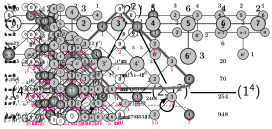
$\hskip 227.62204pt\mathrm{A}=\left(\begin{matrix}0&1&0&0&0\\ 1&1&1&1&0\\ 0&1&0&1&0\\ 0&1&1&1&1\\ 0&0&0&1&0\\ \end{matrix}\right)\ .$

Figure 1: Representation graph $\mathcal{R}_{\mathsf{V}}(\mathbf{S}_{4})$ and its adjacency matrix $\mathrm{A}$ for $\mathsf{V}=\mathbf{S}_{4}^{(3,1)}$

Applying Theorem 2.1 and using the second row of the character table, we have

$$\mathsf{det}(\mathrm{I}-t\mathrm{A}) =\textstyle{\prod_{g\in\Gamma}}\big{(}1-\chi_{(3,1)}(g)\,t\big{)}=(1-3t)(1-t)(1+t)^{2}$$

$$=1-2t-4t^{2}+2t^{3}+3t^{4}.$$

This leads to the following expressions for $\mathsf{m}^{\lambda}(t)=\displaystyle{\frac{\mathsf{det}(\mathrm{M}^{\lambda})}{\mathsf{det}(\mathrm{I}-t\mathrm{A})}}$:

$$\mathsf{m}^{(4)}(t)=\displaystyle{\frac{1-2t-3t^{2}+t^{3}+t^{4}}{1-2t-4t^{2}+2t^{3}+3t^{4}}} =1+t^{2}+t^{3}+4t^{4}+10t^{5}+31t^{6}+\cdots$$

$$\mathsf{m}^{(3,1)}(t)=\displaystyle{\frac{t-t^{2}-2t^{3}}{1-2t-4t^{2}+2t^{3}+3t^{4}}} =t+t^{2}+4t^{3}+10t^{4}+31t^{5}+91t^{6}+\cdots$$

$$\mathsf{m}^{(2^{2})}(t)=\displaystyle{\frac{t^{2}-t^{4}}{1-2t-4t^{2}+2t^{3}+3t^{4}}} =t^{2}+2t^{3}+7t^{4}+20t^{5}+61t^{6}+\cdots$$

$$\mathsf{m}^{(2,1^{2})}(t)=\displaystyle{\frac{t^{2}+t^{3}}{1-2t-4t^{2}+2t^{3}+3t^{4}}} =t^{2}+3t^{3}+10t^{4}+30t^{5}+91t^{6}+\cdots$$

$$\mathsf{m}^{(1^{4})}(t)=\displaystyle{\frac{t^{3}+t^{4}}{1-2t-4t^{2}+2t^{3}+3t^{4}}} =t^{3}+3t^{4}+10t^{5}+30t^{6}+\cdots$$

Next, we connect the Poincaré series for tensor multiplicities in Theorem 2.1 to Bratteli diagrams.

2.3 Bratteli diagrams

The Bratteli diagram $\mathcal{B}_{\mathsf{V}}(\mathsf{G})$ associated to the group $\mathsf{G}$ and the module $\mathsf{V}$ is the infinite graph with vertices labeled by the elements of $\Lambda_{k}(\mathsf{G})$ on level $k$. A walk of $k$ steps on the representation graph $\mathcal{R}_{\mathsf{V}}(\mathsf{G})$ from $0$ to $\lambda$ is a sequence $\left(0,{\lambda^{1}},{\lambda^{2}},\ldots,{\lambda^{k}}=\lambda\right)$ starting at $\lambda^{0}=0$, such that $\lambda^{j}\in\Lambda(\mathsf{G})$ for each $1\leq j\leq k$, and $\lambda^{j-1}$ is connected to ${\lambda^{j}}$ by an edge in $\mathcal{R}_{\mathsf{V}}(\mathsf{G})$. Such a walk is equivalent to a unique path of length $k$ on the Bratteli diagram $\mathcal{B}_{\mathsf{V}}(\mathsf{G})$ from $0$ at the top to $\lambda\in\Lambda_{k}(\mathsf{G})$ on level $k$.

The subscript on vertex $\lambda\in\Lambda_{k}(\mathsf{G})$ in $\mathcal{B}_{\mathsf{V}}(\mathsf{G})$ indicates the number $\mathsf{m}_{k}^{\lambda}$ of paths from $0$ on the top to $\lambda$ at level $k$ (hence, the number of walks on $\mathcal{R}_{\mathsf{V}}(\mathsf{G})$ of $k$ steps from $0$ to $\lambda$). It can be easily computed by summing, in a Pascal triangle fashion, the subscripts of the vertices at level $k-1$ that are connected to $\lambda$. This is the multiplicity of $\mathsf{G}^{\lambda}$ in $\mathsf{V}^{\otimes k}$, which is also the dimension of the irreducible $\mathsf{Z}_{k}(\mathsf{G})$-module $\mathsf{Z}_{k}^{\lambda}$ by Schur-Weyl duality. The sum of the squares of those dimensions at level $k$ is the number on the right, which is the dimension of the centralizer algebra $\mathsf{Z}_{k}(\mathsf{G})$.

The Bratteli diagram for the $\mathbf{S}_{4}$ example in the previous section is displayed in Figure 2 below. The coefficients of the series in (2.2) are the multiplicities $\mathsf{m}_{k}^{\lambda}$, and hence, they are the subscripts on the node $\lambda$ in the Bratteli diagram reading down the column containing $\lambda$. They are the dimensions of the irreducible modules $\mathsf{Z}_{k}^{\lambda}$ for the centralizer algebras $\mathsf{Z}_{k}(\mathbf{S}_{4})=\mathsf{End}_{\mathbf{S}_{4}}(\mathsf{V}^{\otimes k})$ for $\mathsf{V}=\mathbf{S}_{4}^{(3,1)}$ and $k=0,1,\dots$. The sum of the squares of the subscripts in a given row $k$ is the dimension of $\mathsf{Z}_{k}(\mathbf{S}_{4})$ and is the number on the right. The series $\mathsf{m}^{(4)}(t)$ is the Poincaré series for the $\mathbf{S}_{4}$-invariants in $\mathsf{T}(\mathsf{V})=\bigoplus_{k\geq 0}\mathsf{V}^{\otimes k}$. The series $\sum_{k\geq 0}\mathsf{m}_{2k}^{(4)}t^{2k}$, which corresponds to the right-hand column, is the generating function for the dimensions $\,\mathsf{dim}\,\mathsf{Z}_{k}(\mathbf{S}_{4})$ of the centralizer algebras (and also for the $\mathbf{S}_{4}$-invariants in $\mathsf{T}^{\mathsf{even}}(\mathsf{V})=\bigoplus_{k\geq 0}\mathsf{V}^{\otimes(2k)}$ ).

$$\begin{array}[]{c}\includegraphics[scale={1},page=2]{poincare-diagrams.pdf}\end{array}$$

Figure 2: Levels $k=0,1,\dots,6$ of the Bratteli diagram $\mathcal{B}_{\mathsf{V}}(\mathbf{S}_{4})$ for $\mathsf{V}=\mathbf{S}_{4}^{(3,1)}$

3 Poincaré series for the finite subgroups of $\mathsf{SU}_{2}$

When $\mathsf{G}$ is one of the finite subgroups $\mathbf{C}_{n}$, $\mathbf{D}_{n}$, $\mathbf{T}$, $\mathbf{O}$, $\mathbf{I}$ of $\mathsf{SU}_{2}$, and $\mathsf{V}=\mathbb{C}^{2}$, the defining 2-dimensional module for $\mathsf{G}$, we have the following immediate consequence of the McKay correspondence and Theorem 2.1.

Theorem 3.1.

Let $\mathsf{G}$ be a finite subgroup of $\mathsf{SU}_{2}$ and $\mathsf{V}=\mathbb{C}^{2}$. Then the Poincaré series for the $\mathsf{G}$-invariants $\mathsf{T}(\mathsf{V})^{\mathsf{G}}$ in $\mathsf{T}(\mathsf{V})=\bigoplus_{k\geq 0}\mathsf{V}^{\otimes k}$ is

$$\mathsf{m}^{0}(t)=\frac{\mathsf{det}\left(\mathrm{I}-t\mbox{\AA}\right)}{\mathsf{det}\left(\mathrm{I}-t\mathrm{A}\right)}=\frac{\mathsf{det}\left(\mathrm{I}-t\mbox{\AA}\right)}{\prod_{g\in\Gamma}\left(1-\chi_{\mathsf{V}}(g)t\right)},$$ (3.2)

where $\mathrm{A}$ is the adjacency matrix of the representation graph $\mathcal{R}_{\mathsf{V}}(\mathsf{G})$ (i.e. the affine Dynkin diagram corresponding to $\mathsf{G}$ in (1.3));  Å is the adjacency matrix of the finite Dynkin diagram obtained by removing the affine node; and $\chi_{\mathsf{V}}(g)$ is the value of the character $\chi_{\mathsf{V}}$ at $g\in\Gamma$, a set of conjugacy class representatives for $\mathsf{G}$.

Remark 3.3.

Theorem 3.1 can be regarded as an analog of Ebeling’s theorem [E] (see also [Stk, Sec. 5.5]) for finite subgroups $\mathsf{G}$ of $\mathsf{SU}_{2}$, which relates the Poincaré series $\mathsf{s}^{0}(t)$ for the $\mathsf{G}$-invariants in the symmetric algebra $\mathsf{S}(\mathsf{V})=\bigoplus_{k\geq 0}\mathsf{S}^{k}(\mathsf{V})$ to the characteristic polynomial $\mathsf{ch}^{{}^{\boldsymbol{\circ}}}(t)$ (resp. $\mathsf{ch}(t)$) of a Coxeter transformation (resp. of an affine Coxeter transformation) associated to $\mathsf{G}$,

$$\mathsf{s}^{0}(t)=\frac{\mathsf{ch}^{{}^{\boldsymbol{\circ}}}(t)}{\mathsf{ch}(t)}.$$ (3.4)

Coxeter transformations (resp. affine Coxeter transformations) are products of reflections corresponding to the simple roots (resp. affine simple roots). There is one reflection in the product for each node in the finite (resp. affine) Dynkin diagram. There is a close connection between the spectrum of a Coxeter transformation and the spectrum of the associated Cartan matrix $\mathrm{C}$ which was described in [BLM] (see also [C] for Dynkin diagrams with odd cycles). Eigenvalues of $\mathrm{C}$ occur in pairs $\xi,4-\xi$, and for each such a pair, $2-\xi$ and $\xi-2$ are eigenvalues of the adjacency matrix of the Dynkin diagram. The results of [BLM] and [C] (see also [Ste] and the discussion in [D] for the finite diagrams) imply that the eigenvalues of Å (resp. $\mathrm{A}$) are given by $2\cos\left(\pi m/h\right)$ (resp. $2\cos\big{(}\pi\widehat{m}/\widehat{h}\big{)}$) where $m$ (resp. $\widehat{m}$) ranges over the exponents, and $h$ (resp. $\widehat{h}$) is the Coxeter number (resp. affine Coxeter number). In Table 2, we display these exponents and numbers for the simply laced diagrams. For multiply laced diagrams, they can be found in [BLM, Table 1].

Remark 3.5.

In the case not covered in Table 2, namely $\widehat{\mathsf{A}}_{2\ell}$, there are $\ell$ conjugacy classes of Coxeter transformations having different spectra. This case corresponds to the cyclic group $\mathbf{C}_{2\ell+1}$ of odd order, which will be excluded in the next theorem. The characteristic polynomials of the affine Coxeter transformations for $\widehat{\mathsf{A}}_{2\ell}$ have been computed by Coleman [C]. The Poincaré polynomial $\mathsf{m}^{0}(t)$ for all cyclic groups is given in Theorem 3.23 of Section 3.2 below.

Dynkin Exponents Coxeter

diagram number

$$\mathsf{A}_{n-1}$$  

 

1, 4, 5, 7, 8, 11  12

1, 5, 7, 9, 11, 13, 17  18

1, 7, 11, 13, 17, 19, 23, 29  30

 

 

 

0, 2, 2, 3, 4, 4, 6  6

0, 3, 4, 6, 6, 8, 9,12  12

0, 6, 10, 12, 15, 18, 20, 24, 30  30

Table 2: Exponents and Coxeter numbers

Theorem 3.6.

Let $\mathsf{G}$ be a finite subgroup of $\mathsf{SU}_{2}$ such that $\mathsf{G}\not\cong\mathbf{C}_{n}$ for $n$ odd and let $\mathsf{V}=\mathbb{C}^{2}$. Assume $\mathrm{A}$ is the adjacency matrix of the representation graph $\mathcal{R}_{\mathsf{V}}(\mathsf{G})$ (the affine Dynkin diagram) and Å is the adjacency matrix of the corresponding finite Dynkin diagram. Let $\widehat{\Xi}$ (resp. $\Xi$ ) be the set of exponents and $\widehat{h}$ (resp. $h$) be the Coxeter number corresponding to the affine (resp. finite) Dynkin diagram. Then the Poincaré series for the $\mathsf{G}$-invariants $\mathsf{T}(\mathsf{V})^{\mathsf{G}}$ in $\mathsf{T}(\mathsf{V})=\bigoplus_{k\geq 0}\mathsf{V}^{\otimes k}$ is

$$\mathsf{m}^{0}(t)=\frac{\mathsf{det}\left(\mathrm{I}-t\mbox{\AA}\right)}{\mathsf{det}\left(\mathrm{I}-t\mathrm{A}\right)}=\frac{\mathsf{det}\left(\mathrm{I}-t\mbox{\AA}\right)}{\prod_{g\in\Gamma}\left(1-\chi_{\mathsf{V}}(g)t\right)}=\frac{\prod_{m\in\Xi}\left(1-2\cos\left(\frac{\pi m}{h}\right)t\right)}{\prod_{\widehat{m}\in\widehat{\Xi}}\left(1-2\cos\left(\frac{\pi\widehat{m}}{\widehat{h}}\right)t\right)}.$$ (3.7)

Remark 3.8.

It is a consequence of (3.7) that the character values $\chi_{\mathsf{V}}(g)$ as $g$ ranges over a set $\Gamma$ of conjugacy class representatives of $\mathsf{G}$ are exactly the values $2\cos\left(\pi\widehat{m}/\widehat{h}\right)$, where $\widehat{m}$ is an exponent in $\widehat{\Xi}$ and $\widehat{h}$ is the affine Coxeter number.

In subsequent sections, we will derive other closed-form expressions for the Poincaré series $\mathsf{m}^{0}(t)$ for all the finite subgroups of $\mathsf{SU}_{2}$. In the case of the exceptional polyhedral groups $\mathsf{G}$, we also consider the Poincaré series $\mathsf{m}^{\lambda}(t)$ for all $\lambda\in\Lambda(\mathsf{G})$. Korányi [Kor] has shown that the characteristic polynomial of the finite Cartan matrices of types $\mathsf{A,B,C,D}$ have expressions involving Chebyshev polynomials of both the first and second kind. In [D], Damianou has given an expression for the characteristic polynomial of Å for all finite Dynkin diagrams equivalent to the one in the numerator of (3.7) and related these polynomials to Chebyshev polynomials. Since the closed-form expressions discussed here also will involve Chebyshev polynomials, we briefly review some facts about them.

3.1 Chebyshev polynomials

The Chebyshev polynomials $\mathrm{T}_{n}(t)$ of the first kind are a set of orthogonal polynomials defined by the recursion

$$\mathrm{T}_{0}(t)=1,\ \ \ \mathrm{T}_{1}(t)=t,\quad\mathrm{T}_{n+1}(t)=2t\mathrm{T}_{n}(t)-\mathrm{T}_{n-1}(t)\quad\hbox{\rm for all}\ \ n\geq 1.$$

Thus, the first few polynomials for $n\geq 2$ are

$$\mathrm{T}_{2}(t) =2t^{2}-1$$

$$\mathrm{T}_{3}(t) =4t^{3}-3t$$

$$\mathrm{T}_{4}(t) =8t^{4}-8t^{2}+1$$

$$\mathrm{T}_{5}(t) =16t^{5}-20t^{3}+5t$$

$$\mathrm{T}_{6}(t) =32t^{6}-48t^{4}+18t^{2}-1.$$

The Chebyshev polynomials of the first kind play a critical role in approximating functions, where the roots of the polynomials $\mathrm{T}_{n}(t)$, which can be expressed in terms of cosines, are used as nodes in polynomial interpolation. The polynomials have the following closed-form expressions:

$$\mathrm{T}_{n}(t) =\sum_{r=0}^{\lfloor n/2\rfloor}{n\choose{2r}}t^{n-2r}(t^{2}-1)^{r}=t^{n}\sum_{r=0}^{\lfloor n/2\rfloor}{n\choose{2r}}(1-t^{-2})^{r}$$ (3.9)

$$=2^{n-1}\prod_{r=1}^{n}\left(t-\cos\left(\textstyle{\frac{(2r-1)\pi}{2n}}\right)\right),$$ (3.10)

which can be found in [Ri] (see also [D]).

The Chebyshev polynomials $\mathrm{U}_{n}(t)$ of the second kind appear in the study of spherical harmonics in angular momentum theory and in many other areas of mathematics and physics. They have a similar recursive definition,

$$\mathrm{U}_{0}(t)=1,\ \ \ \mathrm{U}_{1}(t)=2t,\quad\mathrm{U}_{n+1}(t)=2t\mathrm{U}_{n}(t)-\mathrm{U}_{n-1}(t)\quad\hbox{\rm for all}\ \ n\geq 1.$$

A slight variation of these polynomials, which arises frequently and will be useful in what follows, are the polynomials $\mathrm{p}_{n}(t)=\mathrm{U}_{n}(t/2)$, which satisfy the relations

$$\mathrm{p}_{0}(t)=1,\ \ \ \mathrm{p}_{1}(t)=t,\quad\mathrm{p}_{n+1}(t)=t\mathrm{p}_{n}(t)-\mathrm{p}_{n-1}(t)\quad\hbox{\rm for all}\ \ n\geq 1.$$ (3.11)

The first few polynomials in these series for $n\geq 2$ are

$$\mathrm{U}_{2}(t)=$$            

           

           

           

            .

The Chebyshev polynomial $\mathrm{U}_{n}(t)$ has simple roots given by $\cos\big{(}\pi r/(n+1)\big{)}$ where $r=1,\dots,n$. Thus, the roots of $\mathrm{p}_{n}(t)$ are $2\cos\big{(}\pi r/(n+1)\big{)}$ for $r=1,\dots,n$. This leads to the explicit expressions for the polynomials $\mathrm{U}_{n}(t)$ given in [Ri] (see also [D, Sec. 6.3]),

$$\mathrm{U}_{n}(t) =\sum_{r=0}^{\lfloor n/2\rfloor}(-1)^{r}{n-r\choose r}(2t)^{n-2r}\ =\ 2^{n}\prod_{r=1}^{n}\left(t-\cos\left(\frac{\pi r}{n+1}\right)\right)$$ (3.12)

$$\mathrm{p}_{n}(t) =\sum_{r=0}^{\lfloor n/2\rfloor}(-1)^{r}{n-r\choose r}\,t^{n-2r}\ =\ \prod_{r=1}^{n}\left(t-2\cos\left(\frac{\pi r}{n+1}\right)\right).$$ (3.13)

There are many identities relating the Chebyshev polynomials of the second kind to those of the first kind. A particularly useful one for our purposes is

$$\mathrm{U}_{n}(t)-\mathrm{U}_{n-2}(t)=2\mathrm{T}_{n}(t).$$ (3.14)

3.2 Cyclic groups

Assume for $n\geq 3$ that

$$\mathrm{z}=\left(\begin{array}[]{cc}\zeta_{n}^{-1}&0\\ 0&\zeta_{n}\end{array}\right)$$ (3.15)

where $\zeta_{n}=e^{2\pi i/n}$, a primitive $n$th root of unity in $\mathbb{C}$, and let $\mathbf{C}_{n}$ be the cyclic subgroup of $\mathsf{SU}_{2}$ generated by $\mathrm{z}$. The irreducible modules for $\mathbf{C}_{n}$ are all one-dimensional and are given by $\mathbf{C}_{n}^{(\ell)}=\mathbb{C}\mathsf{v}_{\ell}$ for $\ell=0,1,\dots,n-1$, where $\mathrm{z}\mathsf{v}_{\ell}=\zeta^{\ell}\mathsf{v}_{\ell}$. Thus, $\Lambda(\mathbf{C}_{n})=\{0,1,\dots,n-1\}$, and $\mathbf{C}_{n}^{(j)}\cong\mathbf{C}_{n}^{(\ell)}$ whenever $j\equiv\ell\,\mathsf{mod}\,n$. The natural $\mathbf{C}_{n}$-module $\mathsf{V}$ of $2\times 1$ column vectors, which $\mathbf{C}_{n}$ acts on by matrix multiplication, can be identified with the module $\mathbf{C}_{n}^{(-1)}\oplus\mathbf{C}_{n}^{(1)}=\mathbf{C}_{n}^{(n-1)}\oplus\mathbf{C}_{n}^{(1)}$. As $\mathsf{G}$ is abelian, the conjugacy class representatives are simply all the elements $\mathrm{z}^{r}$, $r=0,1,\dots,n-1$, of $\mathsf{G}$. The character value for $\mathrm{z}^{r}$ on $\mathsf{V}$ is $\chi_{\mathsf{V}}(\mathrm{z}^{r})=\zeta_{n}^{-r}+\zeta_{n}^{r}=2\cos(2\pi r/n)$. Thus, (3.2) becomes in this case

$$\mathsf{m}^{0}(t)=\frac{\mathsf{det}\left(\mathrm{I}-t\mbox{\AA}\right)}{\mathsf{det}\left(\mathrm{I}-t\mathrm{A}\right)}=\frac{\mathsf{det}\left(\mathrm{I}-t\mbox{\AA}\right)}{\prod_{r=0}^{n-1}\left(1-2\cos\left(\textstyle{\frac{2\pi r}{n}}\right)t\right)}.$$ (3.16)

The matrix Å in this equation is the adjacency matrix of the finite Dynkin diagram of type $\mathsf{A}_{n-1}$ obtained from the Dynkin diagram $\widehat{\mathsf{A}}_{n-1}$ in (1.3) by removing the affine node. Thus, Å is the tridiagonal matrix,

$$\mbox{\AA}=\left(\begin{matrix}0&1&0&\cdots&0\\ 1&0&1&\dots&0\\ \vdots&\ddots&\ddots&\ddots&0\\ 0&\ldots&1&0&1\\ 0&0&\ldots&1&0\end{matrix}\right).$$

Let $\mathrm{a}_{n-1}(t)$ be the determinant $\mathsf{det}\left(\mathrm{I}-t\mbox{\AA}\right)$ in the $\mathsf{A}_{n-1}$-case, and set $\mathrm{a}_{0}(t)=1=\mathrm{a}_{1}(t)$. It is easy to see using cofactor expansion on $\mathrm{I}-t\mbox{\AA}$ that the following recursion relation holds,

$$\mathrm{a}_{n+1}(t)=\mathrm{a}_{n}(t)-t^{2}\mathrm{a}_{n-1}(t)\qquad\hbox{\rm for}\ \ n\geq 1.$$ (3.17)

An easy inductive argument using the recursion relation for the polynomials $\mathrm{p}_{n}(t)$ in (3.11) shows that

$$\mathrm{a}_{n}(t)=t^{n}\mathrm{p}_{n}(t^{-1})\qquad\hbox{\rm for all}\ \ n\geq 0.$$ (3.18)

Since the roots of $\mathrm{p}_{n}(t)$ are $2\cos(\pi r/(n+1))$ for $r=1,\dots,n$, (compare (3.13)), we have

$$\begin{split}\mathrm{a}_{n}(t)&=t^{n}\mathrm{p}_{n}(t^{-1})=t^{n}\prod_{r=1}^{n}\left(t^{-1}-2\cos\left(\frac{\pi r}{n+1}\right)\right)\\ &=\prod_{r=1}^{n}\left(1-2\cos\left(\frac{\pi r}{n+1}\right)\,t\right).\end{split}$$ (3.19)

Then (3.13) implies that $\mathrm{a}_{n}(t)$ has the closed-form expression,

$$\mathrm{a}_{n}(t)=t^{n}\mathrm{p}_{n}(t^{-1})=t^{n}\sum_{r=0}^{\lfloor n/2\rfloor}(-1)^{r}{n-r\choose r}(t^{-1})^{n-2r}=\sum_{r=0}^{\lfloor n/2\rfloor}(-1)^{r}{n-r\choose r}t^{2r}.$$ (3.20)

(Compare the expressions in [D, Sec. 6.3].)

The denominator in (3.16) is also related to Chebyshev polynomials, as cofactor expansion on $\mathrm{I}-t\mathrm{A}$ combined with (3.18) shows that

$$\begin{split}\mathsf{det}\left(\mathrm{I}-t\mathrm{A}\right)&=\mathrm{a}_{n-1}(t)-2t^{2}\mathrm{a}_{n-2}(t)-2t^{n}\\ &=t^{n-1}\mathrm{p}_{n-1}(t^{-1})-2t^{n}\mathrm{p}_{n-2}(t^{-1})-2t^{n}\\ &=t^{n}\left(t^{-1}\mathrm{p}_{n-1}(t^{-1})-\mathrm{p}_{n-2}(t^{-1})\right)-t^{n}\mathrm{p}_{n-2}(t^{-1})-2t^{n}\\ &=t^{n}\left(\mathrm{p}_{n}(t^{-1})-\mathrm{p}_{n-2}(t^{-1})-2\right).\end{split}$$ (3.21)

Then (3.14) and (3.9) imply

$$\mathrm{U}_{n}(t)-\mathrm{U}_{n-2}(t)=2\mathrm{T}_{n}(t)=2\sum_{r=0}^{\lfloor n/2\rfloor}{n\choose 2r}(t^{2}-1)^{r}t^{n-2r},$$

so that

$$\begin{split}\mathsf{det}\left(\mathrm{I}-t\mathrm{A}\right)&=t^{n}\left(\mathrm{p}_{n}(t^{-1})-\mathrm{p}_{n-2}(t^{-1})-2\right)\\ &=2t^{n}\,\sum_{r=0}^{\lfloor n/2\rfloor}{n\choose 2r}\left(\frac{t^{-2}}{4}-1\right)^{r}\left(\frac{t^{-1}}{2}\right)^{n-2r}\ -\ 2t^{n}\\ &=2^{1-n}\sum_{r=0}^{\lfloor n/2\rfloor}{n\choose 2r}(1-4t^{2})^{r}\ -\ 2t^{n}.\end{split}$$ (3.22)

We summarize what we have shown for the cyclic case in the next theorem.

Theorem 3.23.

Assume $\mathsf{G}$ is the cyclic group $\mathbf{C}_{n}$ and let $\mathsf{V}=\mathbb{C}^{2}=\mathbf{C}_{n}^{(-1)}\oplus\mathbf{C}_{n}^{(1)}$. Then the Poincaré series $\mathsf{m}^{0}(t)$ for the $\mathsf{G}$-invariants $\mathsf{T}(\mathsf{V})^{\mathsf{G}}$ in $\mathsf{T}(\mathsf{V})=\bigoplus_{k\geq 0}\mathsf{V}^{\otimes k}$ is given by

$$\begin{split}\mathsf{m}^{0}(t)&=\frac{{\displaystyle{\prod_{r=1}^{n-1}}\Big{(}1-2\cos(\textstyle{\frac{\pi r}{n}})t\Big{)}}}{\displaystyle{\prod_{r=0}^{n-1}}\Big{(}1-2\cos(\textstyle{\frac{2\pi r}{n}})t\Big{)}}=\frac{\displaystyle{\sum_{r=0}^{\lfloor(n-1)/2\rfloor}(-1)^{r}{n-1-r\choose r}t^{2r}}}{\displaystyle{2^{1-n}\sum_{r=0}^{\lfloor n/2\rfloor}{n\choose 2r}(1-4t^{2})^{r}\ -\ 2t^{n}}}.\end{split}$$ (3.24)

Remark 3.25.

When $\mathsf{G}=\mathbf{C}_{n}$ with $n=2(\ell+1)$ and $\ell\geq 1$, the cosine expression for $\mathsf{m}^{0}(t)$ in (3.24) gives the same result as Theorem 3.6. Indeed, $n-1=2\ell+1$,   $\cos\left(\pi m/(\ell+1)\right)=\cos\left(2\pi m/n\right)$, and the product of the factors   $\left(1-2\cos\left(\pi m\ (\ell+1)\right)t\right)$   as $m$ ranges over the elements of   $\widehat{\Xi}\,=\,\{0,1,1,\dots,\,\ell,\break\ell,\,\ell+1\}$ is the same as the product of the terms $\left(1-2\cos\left(2\pi r/n\right)t\right)$ for $r=0,1,\dots,n-1$, since $\cos\left(2\pi(n-r)/n\right)=\cos\left(2\pi r/n\right)$ for all $r=0,1,\dots,\ell$.

In Table 3, the numerator and denominator polynomials in (3.24) and the Poincaré series $\mathsf{m}^{0}(t)$ are displayed for $\mathbf{C}_{n}$, $n=3,4,5,6,7$.

$$\mathsf{det}(\mathrm{I}-t\mbox{\AA})$$

Table 3: Poincaré series $\mathsf{m}^{0}(t)$ for the cyclic groups $\mathbf{C}_{n}$,   $3\leq n\leq 7$

The Bratteli diagram for $\mathbf{C}_{n}$ and $\mathsf{V}=\mathbb{C}^{2}$ is Pascal’s triangle on a cylinder of “diameter” $\tilde{n}$, where $\tilde{n}=n$ if $n$ is odd and $\tilde{n}=\frac{1}{2}n$ if $n$ is even. Pictured in Figure 3 is the Bratteli diagram for $\mathbf{C}_{5}$. The subscripts on the white (trivial) node correspond to the Poincaré series $1+2t^{2}+6t^{4}+2t^{5}+20t^{6}+14t^{7}+\cdots$ in the third line of Table 3.

$$\begin{array}[]{c}\includegraphics[scale={.7},page=6]{poincare-diagrams.pdf}\end{array}$$

Figure 3: Levels $k=0,1,\dots,6$ of the Bratteli diagram $\mathcal{B}_{\mathsf{V}}(\mathbf{C}_{5})$ for $\mathsf{V}=\mathbb{C}^{2}$

Remark 3.26.

It was shown in [BBH, Sec. 1.6] by using the basic construction of Jones [J1] that for all finite subgroups $\mathsf{G}$ of $\mathsf{SU}_{2}$, the edges in $\mathcal{B}_{\mathsf{V}}(\mathsf{G})$ between level $k$ and level $k+1$ that are NOT obtained from edges between level $k-1$ and level $k$ by reflection over level $k$, exactly form the representation graph (affine Dynkin diagram), except in the $\mathbf{C}_{n}$ case for $n$ odd where it is the double of the Dynkin diagram. This is indicated by the shaded edges in Figures 3, 4, 5, 6, and 7 below and has important implications for the structure of the centralizer algebras $\mathsf{Z}_{k}(\mathsf{G})$.

3.3 Binary dihedral groups

Assume for $n\geq 2$, that

$$\mathrm{x}=\left(\begin{array}[]{cc}\zeta_{2n}^{-1}&0\\ 0&\zeta_{2n}\end{array}\right)\quad\hbox{\rm and}\quad\mathrm{y}=\left(\begin{array}[]{cc}0&i\\ i&0\end{array}\right),$$ (3.27)

where $i=\sqrt{-1}$ and $\zeta_{2n}=e^{2\pi i/2n}=e^{\pi i/n}$, a primitive $2n$th root of unity. The elements $\mathrm{x}$ and $\mathrm{y}$ generate a binary dihedral subgroup $\mathbf{D}_{n}$ of order $4n$ in $\mathsf{SU}_{2}$. There are four irreducible $\mathbf{D}_{n}$-modules of dimension $1$, and $n-1$ irreducible modules of dimension $2$. The defining module $\mathsf{V}=\mathbb{C}^{2}$ is irreducible as a $\mathbf{D}_{n}$-module.

We take as the conjugacy class representatives of $\mathbf{D}_{n}$ the elements in $\Gamma=\{\pm\mathrm{I},\ \mathrm{x}^{r},(r=1,\dots,n-1),\mathrm{y},\ \mathrm{yx}\}$ . Then computing their traces gives

$$\mathsf{det}\left(\mathrm{I}-t\mathrm{A}\right) =\prod_{g\in\Gamma}\left(1-\chi_{\mathsf{V}}(g)t\right)=(1-2t)(1+2t)\prod_{r=1}^{n-1}\left(1-2\cos\left(\frac{\pi r}{n}\right)t\right)$$

$$=(1-4t^{2})\mathrm{a}_{n-1}(t)=(1-4t^{2})\sum_{r=0}^{\lfloor(n-1)/2\rfloor}(-1)^{r}{n-1-r\choose r}t^{2r},$$ (3.28)

where the expression for $\mathrm{a}_{n-1}(t)$ follows from (3.20).

The matrix Å is the adjacency matrix of the finite Dynkin diagram of type $\mathsf{D}_{n+2}$ obtained from the Dynkin diagram $\widehat{\mathsf{D}}_{n+2}$ in (1.3). Let $\mathrm{d}_{n}(t)$ be the determinant $\mathsf{det}\left(\mathrm{I}-t\mbox{\AA}\right)$ in the $\mathsf{D}_{n+2}$-case, and set $\mathrm{d}_{0}(t)=1,\ \mathrm{d}_{1}(t)=1-2t^{2}$. It is easy to see using cofactor expansion on the matrix $\mathrm{I}-t\mbox{\AA}$ that the following recursion relation holds,

$$\mathrm{d}_{n+1}(t)=\mathrm{d}_{n}(t)-t^{2}\mathrm{d}_{n-1}(t)\qquad\hbox{\rm for}\ \ n\geq 1.$$

The polynomials $2t^{n+1}\mathrm{T}_{n+1}(t^{-1}/2)$, where $\mathrm{T}_{n+1}(t)$ is the Chebyshev polynomial of the first kind, satisfy the same initial conditions; namely,

$$2t^{n+1}\mathrm{T}_{n+1}\left(\frac{t^{-1}}{2}\right)=\begin{cases}1&\qquad\hbox{\rm for}\ \ n=0\\ 1-2t^{2}&\qquad\hbox{\rm for}\ \ n=1,\end{cases}$$

and the same recursion relation as the polynomials $\mathrm{d}_{n}(t)$. As a consequence, we can conclude

$$\mathrm{d}_{n}(t)=2t^{n+1}\mathrm{T}_{n+1}\left(\frac{t^{-1}}{2}\right).$$

Combining that relation with the identities in (3.9) and (3.10) gives

$$\mathrm{d}_{n}(t) =2t^{n+1}\left(\frac{t^{-1}}{2}\right)^{n+1}\sum_{r=0}^{\lfloor{n+1}/2\rfloor}{n+1\choose{2r}}\left(1-\left(\frac{t^{-1}}{2}\right)^{-2}\right)^{r}$$

$$=2^{-n}\sum_{r=0}^{\lfloor(n+1)/2\rfloor}{n+1\choose{2r}}(1-4t^{2})^{r}$$ (3.29)

$$=\prod_{r=1}^{n+1}\left(1-2\cos\left(\textstyle{\frac{(2r-1)\pi}{2(n+1)}}\right)t\right).$$ (3.30)

(Compare with [D, Sec. 6.5], which computes the characteristic polynomial of Å for the $\mathsf{D}$-case.) The expressions in (3.29) and (3.30) together with (3.3) imply the next result.

Theorem 3.31.

Assume $\mathsf{G}$ is the binary dihedral group $\mathbf{D}_{n}$, and let $\mathsf{V}=\mathbb{C}^{2}$. Then the Poincaré series $\mathsf{m}^{0}(t)$ for the $\mathsf{G}$-invariants in $\mathsf{T}(\mathsf{V})=\bigoplus_{k\geq 0}\mathsf{V}^{\otimes k}$ is given by

$$\mathsf{m}^{0}(t) =\frac{2t^{n+1}\mathrm{T}_{n+1}\left(\frac{t^{-1}}{2}\right)}{(1-4t^{2})\displaystyle{\prod_{r=1}^{n-1}}\Big{(}1-2\cos(\textstyle{\frac{\pi r}{n}})t\Big{)}}=\frac{\displaystyle{\prod_{r=1}^{n+1}}\left(1-2\cos\left(\textstyle{\frac{(2r-1)\pi}{2(n+1)}}\right)t\right)}{(1-4t^{2})\displaystyle{\prod_{r=1}^{n-1}}\Big{(}1-2\cos(\textstyle{\frac{\pi r}{n}})t\Big{)}}$$ (3.32)

$$=\frac{\displaystyle{2^{-n}\sum_{r=0}^{\lfloor(n+1)/2\rfloor}{n+1\choose{2r}}(1-4t^{2})^{r}}}{(1-4t^{2})\displaystyle{\sum_{r=0}^{\lfloor(n-1)/2\rfloor}(-1)^{r}{n-1-r\choose r}t^{2r}}}.$$

Table 4 below displays the polynomials $\mathsf{det}(\mathrm{I}-t\mbox{\AA})$ and $\mathsf{det}(\mathrm{I}-t\mathrm{A})$ and Poincaré series $\mathsf{m}^{0}(t)=\mathsf{det}\left(\mathrm{I}-t\mbox{\AA}\right)/\mathsf{det}\left(\mathrm{I}-t\mathrm{A}\right)$ for $\mathbf{D}_{n}$, $n=2,3,4,5,6$. The Bratteli diagram for the binary dihedral group $\mathbf{D}_{6}$ and $\mathsf{V}=\mathbb{C}^{2}$ is pictured in Figure 4. The shaded edges give the representation graph (affine Dynkin diagram $\widehat{\mathsf{D}}_{8}$). The subscripts on the white node, which corresponds to the trivial $\mathbf{D}_{6}$-module, are the coefficients of the Poincaré series $\mathsf{m}^{0}(t)$ in the last line of Table 4.

	$\mathsf{det}(\mathrm{I}-t\mbox{\AA})$	$\mathsf{det}(\mathrm{I}-t\mathrm{A})$	$\mathsf{m}^{0}(t)$
$(\mathbf{D}_{2},\widehat{\mathsf{D}}_{4})$	$1-3t^{2}$	$1-4t^{2}$	$1+t^{2}+4t^{4}+16t^{6}$
			$+64t^{8}+256t^{10}+\,\cdots\,$
$(\mathbf{D}_{3},\widehat{\mathsf{D}}_{5})$	$1-4t^{2}+2t^{4}$	$1-5t^{2}+4t^{4}$	$1+t^{2}+3t^{4}+11t^{6}$
			$43t^{8}+171t^{10}\,+\,\cdots$
$(\mathbf{D}_{4},\widehat{\mathsf{D}}_{6})$	$1-5t^{2}+5t^{4}$	$1-6t^{2}+8t^{4}$	$1+t^{2}+3t^{4}+10t^{6}$
			$+36t^{8}+136t^{10}\,+\,\cdots$
$(\mathbf{D}_{5},\widehat{\mathsf{D}}_{7})$	$1-6t^{2}$	$1-7t^{2}$	$1+t^{2}+3t^{4}+10t^{6}$
	$+9t^{4}-2t^{6}$	$+13t^{4}-4t^{6}$	$35t^{8}+118t^{10}\,+\,\cdots$
$(\mathbf{D}_{6},\widehat{\mathsf{D}}_{8})$	$1-7t^{2}$	$1-8t^{2}$	$1+t^{2}+3t^{4}+10t^{6}$
	$+14t^{4}-7t^{6}$	$+19t^{4}-12t^{6}$	$+35t^{8}+126t^{10}\,+\,\cdots$

Table 4: Poincaré series $\mathsf{m}^{0}(t)$ for the binary dihedral groups $\mathbf{D}_{n}$,   $2\leq n\leq 6$

$$\begin{array}[]{c}\includegraphics[scale={.75},page=7]{poincare-diagrams.pdf}\end{array}$$

Figure 4: Levels $k=0,1,\dots,8$ of the Bratteli diagram $\mathcal{B}_{\mathsf{V}}(\mathbf{D}_{6})$ for $\mathsf{V}=\mathbb{C}^{2}$

3.4 Exceptional binary polyhedral groups

In this final section, we present analogous results for the subgroups $\mathbf{T},\mathbf{O},$ and $\mathbf{I}$ of $\mathsf{SU}_{2}$. The denominator $\mathsf{det}(\mathrm{I}-t\mathrm{A})$ in the Poincaré series can be computed by applying Theorem 3.6 with the exponents in Table 2. Alternatively, one can use the fact that $\mathsf{det}(\mathrm{I}-t\mathrm{A})=\prod_{g\in\Gamma}(1-\chi_{\mathsf{V}}(g)t)$ and read off the character values, for example, from [Stk, Tables A.9, A.12, and A.19]. The determinants $\mathsf{det}(\mathrm{I}-t\mathrm{A})$ and $\mathsf{det}(\mathrm{I}-t\mbox{\AA})$ also can be computed by hand or by using a convenient software package. In applying Theorem 3.6 to evaluate $\mathsf{det}(\mathrm{I}-t\mbox{\AA})$, it is helpful to use the fact that the exponents of the finite Dynkin diagram occur in pairs $m,m^{\prime}$ such that $m+m^{\prime}=h$ and $\cos\left(\pi m/h\right)=-\cos\left(\pi m^{\prime}/h\right)$ to get the results below. In Table 5, $\phi=\frac{1}{2}(1+\sqrt{5})$ (the golden ratio), and $\phi^{*}=\frac{1}{2}(1-\sqrt{5})$. The subscripts on the white (trivial) nodes in the Bratteli diagrams $\mathcal{B}_{\mathsf{V}}(\mathsf{G})$ below for $\mathsf{G}=\mathbf{T},\mathbf{O},\mathbf{I}$ correspond to the coefficients of Poincaré series $\mathsf{m}^{0}(t)$ in Table 5.

$$(\mathbf{T},\widehat{\mathsf{E}}_{6})$$

    

      

Table 5: Poincaré series $\mathsf{m}^{0}(t)=\mathsf{det}(\mathrm{I}-t\mbox{\AA})/\mathsf{det}(\mathrm{I}-t\mathrm{A})$ for the exceptional polyhedral groups

Figure 5: Levels $k=0,1,\dots,8$ of the Bratteli diagram $\mathcal{B}_{\mathsf{V}}(\mathbf{T})$ for $\mathsf{V}=\mathbb{C}^{2}$

Figure 6: Levels $k=0,1,\dots,8$ of the Bratteli diagram $\mathcal{B}_{\mathsf{V}}(\mathbf{O})$ for $\mathsf{V}=\mathbb{C}^{2}$

Figure 7: Levels $k=0,1,\dots,8$ of the Bratteli diagram $\mathcal{B}_{\mathsf{V}}(\mathbf{I})$ for $\mathsf{V}=\mathbb{C}^{2}$

Recall from (2.2) that the Poincaré series $\mathsf{m}^{\mu}(t)$ for the multiplicity of the irreducible $\mathsf{G}$-module $\mathsf{G}^{\mu}$ in the tensor algebra $\mathsf{T}(\mathsf{V})$ is given by $\mathsf{m}^{\mu}(t)=$ $\mathsf{det}(\mathrm{M}^{\mu})/\mathsf{det}(\mathrm{I}-t\mathrm{A})=\mathsf{det}(\mathrm{M}^{\mu})/\prod_{g\in\Gamma}\left(1-\chi_{\mathsf{V}}(g)t\right)$, where $\mathrm{M}^{\mu}$ is the matrix obtained from $\mathrm{I}-t\mathrm{A}$ by replacing the column indexed by $\mu$ by the column $\underline{\delta}=\left(\begin{smallmatrix}1\\ 0\\ \vdots\\ \\ 0\end{smallmatrix}\right)$ in Theorem 2.1. The series $\mathsf{m}^{\mu}(t)$ can also be computed using Remark 2.4 since $\mathsf{m}^{0}(t)$ is known from Table 5. In the diagrams below, we attach to each node $\mu$ of the affine Dynkin diagrams $\widehat{\mathsf{E}}_{6},\widehat{\mathsf{E}}_{7},\widehat{\mathsf{E}}_{8}$, the polynomial $\mathsf{det}(\mathrm{M}^{\mu})$. The polynomial for $\mu=0$ is the same as $\mathsf{det}(\mathrm{I}-t\mbox{\AA})$ in the previous table.

Figure 8:   $\mathsf{det}(\mathrm{M}^{\mu})$ for the binary tetrahedral and octahedral groups $\mathbf{T}$ and $\mathbf{O}$

Figure 9:   $\mathsf{det}(\mathrm{M}^{\mu})$ for the binary icosahedral group $\mathbf{I}$

Remark 3.33.

An inductive argument on the edge connections in the Bratteli diagram can be used to determine formulas for the irreducible $\mathsf{Z}_{k}(\mathsf{G})$-modules (i.e. for the multiplicities $\mathsf{m}_{k}^{\lambda}$) for the exceptional polyhedral groups. The results of applying this method were given in [BBH]. For example, when $\lambda=0$, then $\mathsf{m}_{k}^{0}=0$ unless $k$ is even, and for $k=2n\geq 2$, we have from [BBH, Sec. 4.3] that

$$\mathsf{m}_{k}^{0}=\begin{cases}\frac{1}{12}(4^{n}+8)&\qquad\hbox{\rm if}\ \ \mathsf{G}=\mathbf{T},\\ \frac{1}{24}(4^{n}+6\cdot 2^{n}+8)&\qquad\hbox{\rm if}\ \ \mathsf{G}=\mathbf{O},\\ \frac{1}{60}(4^{n}+12\mathsf{L}_{2n}+20)&\qquad\hbox{\rm if}\ \ \mathsf{G}=\mathbf{I},\end{cases}$$

where $L_{2n}$ is the (2n)th Lucas number. The Lucas numbers $L_{r}$, $r\geq 0$, satisfy the Fibonacci recursion $L_{r+1}=L_{r}+L_{r-1}$ but start from the initial conditions $L_{0}=2,\ L_{1}=1$. Similar expressions for $\mathsf{m}_{k}^{\lambda}$ for all $\lambda\in\Lambda(\mathbf{I})$ also involve Lucas numbers. The expressions for $\mathsf{m}_{k}^{\lambda}$ in [BBH, Sec. 4.3] can be put into a generating series, which can also be used to determine the Poincaré series $\mathsf{m}_{k}^{\lambda}(t)$ for the exceptional groups.

Department of Mathematics, University of Wisconsin-Madison, Madison, WI 53706, USA
benkart@math.wisc.edu

References

• [BBH] J.M. Barnes, G. Benkart, and T. Halverson, McKay centralizer algebras, Proc. Lond. Math. Soc. to appear; arXiv #1213.5254.
• [Be] G Benkart, Connecting the McKay correspondence and Schur-Weyl duality, Proceedings of International Congress of Mathematicians Seoul 2014, Vol. 1, 633–656.
• [BH] G. Benkart and T. Halverson, Exceptional McKay centralizer algebras, in preparation.
• [BLM] S. Berman, S. Lee, and R.V. Moody, The spectrum of a Coxeter transformation, affine Coxeter transformations, and the defect map, J. Algebra 121 (1989), 339–357.
• [Bo] N. Bourbaki, Groupes et Algèbres de Lie, Ch. 4-6, Hermann, Paris, 1968; Masson Paris 1981.
• [BDO] C. Bowman, M. DeVisscher, and R. Orellana, The partition algebra and the Kronecker coefficients, Trans. Amer. Math. Soc. 367 (2015), no. 5, 3647–3667.
• [C] A.J.. Coleman, Killing and the Coxeter transformation of Kac-Moody algebras, Invent. Math. 95 (1989), 447–477.
• [D] P.A. Damianou, On the characteristic polynomial of Cartan matrices and Chebyshev polynomials, arXiv #1110.6620v2.
• [E] W. Ebeling, Poincaré series and monodromy of a two-dimensional quasi-homogeneous hypersurface singularity, Manuscripta Math. 107 (2002), no. 3, 271–282.
• [G-SV] G. Gonzalez-Sprinberg and J.L. Verdier, Construction geometrique de la correspondence de McKay, Ann. Sci. École Norm. Sup. (4) 16 (1983), no. 3, 409–449.
• [HR] T. Halverson and A. Ram, Partition algebras, European J. Combin. 26 (2005), no. 6, 869–921.
• [J1] V.F.R. Jones, Index for subfactors, Invent. Math. 72 (1983), 1–25.
• [J2] V.F.R. Jones, The Potts model and the symmetric group, in: Subfactors: Proceedings of the Taniguchi Symposium on Operator Algebras (Kyuzeso, 1993), World Scientific Publishing, River Edge, N.J., 1994, pp. 259–267.
• [Ka] V.G. Kac, Infinite-dimensional Lie Algebras, 3rd ed., Cambridge Univ. Press, Cambridge, 1990.
• [Kn] H. Knörrer, Group representations and the resolution of rational double points, Finite Groups - Coming of Age, Cont. Math. 45 (1985), 175–222.
• [Kor] A. Korányi, Spectral properties of the Cartan matrices, Acta Sci. Math. (Szeged) 57 (1993), no. 1-4, 587–592.
• [Kos1] B. Kostant, On finite subgroups of SU(2), simple Lie algebras, and the McKay correspondence, Proc. Nat. Acad. Sci. U.S.A. 81 (1984), no. 16, Phys. Sci., 5275–5277.
• [Kos2] B. Kostant, The McKay correspondence, the Coxeter element and representation theory, The mathematical heritage of Elie Cartan (Lyon 1984), Asterisque 1985, Numéro Hors Série, 209–255.
• [Kos3] B. Kostant, The Coxeter element and the branching law for the finite subgroups of SU(2), “The Coxeter Legacy” 63–70, Amer. Math. Soc., Providence, R.I. 2006.
• [M1] P.  Martin, Representations of graph Temperley-Lieb algebras, Publ. Res. Inst. Math. Sci. 26 (1990) no. 3, 485–503.
• [M2] P. Martin, The structure of the partition algebra, J. Algebra 183 (1996) 319–358.
• [Mc1] J. McKay, Graphs, singularities, and finite groups, The Santa Cruz Conference on Finite Groups (Univ. California, Santa Cruz, Calif., 1979), pp. 183–186, Proc. Sympos. Pure Math., 37, Amer. Math. Soc., Providence, R.I., 1980.
• [Mc2] J. McKay, Cartan matrices, finite groups of quaternions, and Kleinian singularities, Proc. Amer. Math. Soc. 81 (1981), no. 1, 153–154.
• [Mc3] J. McKay, Semi-affine Coxeter-Dynkin graphs and $G\subseteq SU_{2}(\mathbb{C})$, Canad. J. Math. 51 (1999), no. 6, 1226–1229.
• [Ri] T.J. Rivlin, Chebyshev Polynomials. From Approximation Theory to Algebra and Number Theory, Pure and Applied Mathematics (New York). John Wiley & Sons, Inc., New York, 1990.
• [Ro] W. Rossmann, McKay’s correspondence and characters of finite subgroups of SU(2), Noncommutative Harmonic Analysis, 441–458, Progr. Math. 220, Birkhäuser Boston, Boston, MA 2004.
• [Sl1] P. Slodowy, Simple Singularities and Simple Algebraic Groups, Lecture Notes in Mathematics 815, Springer, Berlin, 1980.
• [Sl2] P. Slodowy, Platonic solids, Kleinian singularities, and Lie groups, Algebraic Geometry (Ann Arbor, Mich., 1981) 102-138, Lecture Notes in Math. 1008, Springer, Berlin, 1983.
• [Sp1] T.A. Springer, Poincaré series of binary polyhedral groups and McKay’s correspondence, Math. Ann. 278 (1987), 99–116.
• [Sp2] T.A. Springer, Some remarks on characters of the binary polyhedral groups, J. Algebra 131 (1990), 641–647.
• [Ste] R. Steinberg, Finite subgroups of $\mathsf{SU}_{2}$, Dynkin diagrams and affine Coxeter elements, Pacific J. Math. 118 (1985), no. 2, 587–598.
• [Stk] R. Stekolshchik, Notes on Coxeter Transformations and the McKay Correspondence, Springer Monographs in Mathematics, Springer-Verlag, Berlin, 2008.
• [Su] R. Suter, Quantum affine Cartan matrices, Poincaré series of binary polyhedral groups, and reflection representations, Manuscripta Math. 122 (2007), 1–21.