Nuclear Pasta Matter for Different Proton Fractions

Abstract

Nuclear matter under astrophysical conditions is explored with time-dependent and static Hartree-Fock calculations. The focus is in a regime of densities where matter segregates into liquid and gaseous phases unfolding a rich scenario of geometries, often called nuclear pasta shapes (e.g. spaghetti, lasagna). Particularly the appearance of the different phases depending on the proton fraction and the transition to uniform matter are investigated. In this context the neutron background density is of special interest, because it plays a crucial role for the type of pasta shape which is built. The study is performed in two dynamical ranges, once for hot matter and once at temperature zero to investigate the effect of cooling.

I Introduction

Nuclear matter in supernova cores and proto-neutron stars covers a wide range of density, temperature, and proton fraction, and hence exhibits various interesting properties such as, e.g., liquid-gas mixing Lamb et al. (1978). It is believed that after the bounce of the inner core, cooling and deleptonization lead to drastic changes in the temperature and proton fraction of each matter element inside the core Bethe (1990); Suzuki (1994). Just below normal nuclear density, matter is likely to disentangle into exotic shapes, which resemble pastas like spaghetti and lasagna and can affect neutrino transport Ravenhall et al. (1983); Hashimoto et al. (1984); Lassaut et al. (1987); Pethick and Ravenhall (1995); Chamel and Haensel (2008); Horowitz et al. (2004a, b); Sonoda et al. (2007). Steadily increasing computing power allows meanwhile to simulate pasta matter by fully three-dimensional, symmetry unrestricted time-dependent Hartree-Fock (TDHF) calculations. This has led to a revival of investigations of structure and dynamics of pasta matter within TDHF Newton and Stone (2009); Sébille et al. (2009, 2011); Pais and Stone (2012); Schuetrumpf et al. (2013) as well as classical and quantum molecular dynamics calculations Sonoda et al. (2008); Schneider et al. (2013). In this contribution, we address the question how the map of pasta shapes changes with the proton fraction and how the neutron excess is distributed between the nuclear liquid and a gaseous neutron background. Nuclear pasta matter for different values of the proton fraction has been studied so far using classical molecular dynamics Dorso et al. (2012), the TDHF-like DYWAN modelSébille et al. (2011), and a Thomas-Fermi approximation based on a relativistic mean-field model Okamoto et al. (2013). Here we aim at a fully quantum mechanical TDHF description. We thus extend our previous TDHF calculations for proton fraction 1/3 Schuetrumpf et al. (2013) to the general case of arbitrary proton fractions. Thereby we concentrate on the regime of low densities up to saturation density of symmetric nuclear matter. We consider phases at high temperature in the MeV range which are relevant for core-collapse super-novae as well as phases at zero temperature which have relevance to materials that deleptonize in proto-neutron stars.

For the calculations done here the Skyrme-TDHF code as explained in Maruhn et al. (2014) is used. For the astrophysical calculations periodic boundary conditions are assumed. For the interaction the Skyrme force SLy6 is taken Chabanat et al. (1998). Additionally to the proton charge distribution we take a uniform electron background to keep the charge neutrality.

II Simulation and basic quantities

Static and dynamic properties of inhomogeneous nuclear matter are computed with the TDHF code. For the astrophysical calculations performed here, periodic boundary conditions are applied, thus simulating infinite matter approximately with a periodic lattice of simulation boxes. The imposed periodicity exerts a constraint on the system which, in turn, may shift a bit the transition points from one phase to another. We have checked the impact of box size earlier Schuetrumpf et al. (2013) and find that effects are not dramatic for the simple geometries discussed here, although box size can become an issue when dealing with involved shapes as, e.g., gyroids Schuetrumpf et al. (2014). The actual simulation box uses a grid spacing of 1 fm and 16$\times$16$\times$16 grid points thus having a box length $l=16$ fm and a box volume $V=l^{3}$. We vary the number of $\alpha$-particles $N_{\alpha}$, and of additional neutrons $N_{n+}$. The Coulomb field in a periodic simulation is given by the Ewald sum Ewald (1921). The Fourier representation of kinetic energy allows a very elegant computation in Fourier space. Total charge neutrality is achieved by assuming a homogeneous electron background. This approximation ignores screening effects from the electrons, for detailed discussions see Maruyama et al. (2005); Watanabe and Iida (2003); Dorso et al. ; Alcain et al. (2014). Although screening lengths can vary in a wide range and are occasionally of the order of structure size, the net effect of electron screening is found to be small Maruyama et al. (2005); Watanabe and Iida (2003), thus justifying the homogeneous approximation for the present exploration.

The initial state is prepared in similar fashion as in Schuetrumpf et al. (2013). From the $N_{p}$ protons together with $N_{p}$ neutrons, we form $N_{\alpha}=N_{p}/2$ $\alpha$-particles. These are distributed stochastically over the whole space of the simulation box while keeping a minimal distance of ${3.5\rm\,fm}$ between the centers of the $\alpha$-particles to avoid too large overlaps between them. The $\alpha$-particles are initialized at rest. The remaining $N_{n}-N_{p}$ neutrons are initialized as plane waves filling successively the states with the lowest kinetic energies with degenerate pairs of spin-up and spin-down particles. Finally, all nucleons are ortho-normalized. The then following time evolution of the system is done by standard TDHF propagation Maruhn et al. (2014).

This initial state is far above the ground state. During the first few fm/c of dynamical evolution, the system quickly evolves into a fluctuating thermal state whose average properties (shapes, densities, energies) remain basically constant. The emerging temperatures end up in a range well representing pasta matter in core-collapse supernovae. They lie between 2 and 7 MeV depending on proton fraction $X_{p}$ and density $\rho$ where lower $X_{p}$ and larger $\rho$ are found to be associated with lower temperatures. For the present exploratory stage, we use just this broad temperature range as representatives of hot matter. In a second step, we cool down the system for each $X_{p}$ and density $\rho$ to a locally stable zero-temperature state. To that end, we start from a given dynamical state and perform a static calculation with standard techniques of the code Maruhn et al. (2014). The starting configuration is taken from some time point in the late phases of the TDHF simulation. The precise time is unimportant for the final result. The whole procedure (random initialization, evaluation of thermal state, cooling) is done twice for each setting of $X_{p}$ and $\rho$. This gives some clue on the stability of a configuration.

A word is in order about the analysis of non-homogeneous structures of infinite systems in a finite simulation box. It is known that the imposed boundary conditions have an impact on the structures due to symmetry violation and possibly spatial mismatch Hockney and Eastwood (1981); Allen and Tildesley (1987). A study within classical molecular dynamics without Coulomb interactions implies that this may be particularly critical for extended, inhomogeneous structures Molinelli et al. (2014). However, the numerical expense of fully quantum-dynamical simulations sets limits on the affordable box sizes. To check its effect, we have studied for the case of $X_{p}=1/3$ also larger boxes up to 26 fm and find the same structures. Thus we confine the exploratory survey here to the one box size 16 fm.

In order to characterize the matter, we will use a few global properties. The total number of protons and neutrons is

$$N_{p}=2N_{\alpha}\quad,\quad N_{n}=2N_{\alpha}+N_{n+}$$ (1)

where $N_{\alpha}$ is the number of initial $\alpha$ particles (strictly related to $N_{p}$) and $N_{n+}$ the number of excess neutrons (not absorbed into initial $\alpha$ particles). The key parameter is the proton fraction $X_{p}$

$$X_{p}=\frac{N_{p}}{N_{p}+N_{n}}=\frac{2N_{\alpha}}{2N_{\alpha}+N_{n+}}\leq\frac{1}{2}\quad.$$ (2)

The latter inequality means that we confine studies to neutron rich systems which is the typical scenario in astrophysical environment. There are several further measures related to densities. The most important one is the mean density

$$\rho=\frac{N_{p}+N_{n}}{V}=\frac{4N_{\alpha}+N_{n+}}{V}=\frac{A}{V}$$ (3)

where $V$ is the box volume and $A=N_{p}+N_{n}$ is the total nucleon number. It is only at high densities that matter stays homogeneous. Usually, matter segregates into dense regions of nuclear liquid with density $\rho_{l}$ and a dilute gas phase with density $\rho_{g}$, consisting here of a neutron gas. These two phases fill correspondingly volumes $V_{l}$ and $V_{g}$ with $V_{l}+V_{g}=V$. These volumes are defined with the help of the Gibbs dividing surface Shchukin et al. (2001). A threshold density $\rho_{\mathrm{thr}}$ is set and all regions with $\rho(\mathbf{r})>\rho_{\mathrm{thr}}$ are added to $V_{l}$ and all other to $V_{g}$. The threshold is determined such that

$$\rho_{l}\cdot V_{l}+\rho_{g}\cdot V_{g}=A\quad.$$ (4)

From these volumes, the volume fraction $u_{l}$ of the liquid phase can be deduced as

$$u_{l}=\frac{V_{l}}{V}=\frac{\rho-\rho_{g}}{\rho_{l}-\rho_{g}}\quad.$$ (5)

Since $\rho$ is always smaller than $\rho_{l}$ for pasta shapes and the gas density consists of the background densities, the volume fraction becomes smaller for larger neutron background densities and the type of pasta shape which is formed depends strongly on this volume fraction.

The volume fraction $u_{l}$ is the most important parameter to determine the geometry of the system. With steadily increasing $u_{l}$, the system marches through a series of geometrical phases. For the lowest $u_{l}$ the individual shapes are the sphere, which corresponds to finite nuclei with large zones of vacuum around. In the next stage, the nuclei fuse to cylinder-like shapes, the “rod” structure, also denoted as “spaghetti”. Further increasing $u_{l}$ leads to planar meshes of orthogonal rods, “rod(2)”, followed by three-dimensional grids of rods, denoted “rod(3)”. Equally densely packed is the “slab” structure, parallel planes completely filled with matter, also called in a more appetizing manner “lasagna”. From then on the picture is reversed. We have more matter than voids. The slab and rod(3) are symmetric under exchange of matter and voids, thus residing at the turning point. Further increasing $u_{l}$ then yields the phases of “rod(2) bubble”, “rod bubble”, and “sphere bubble”, where bubble denotes that the gas phase has the shape of the pasta. A further increase ends up in homogeneous matter. These are the phases which we will study in the following.

III Results

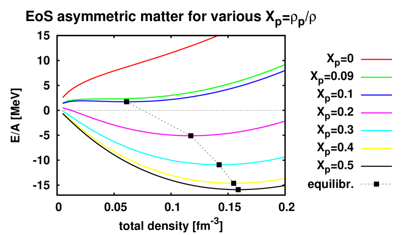
Figure 1: (Color online) Binding energy per particle $E/A$ as function of total density for asymmetric nuclear matter at zero temperature for various proton fractions $X_{p}$ as indicated. The ground states are indicated by black boxes for those $X_{p}$ where a local minimum could be found. The curves have been computed for the Skyrme force SLy6.

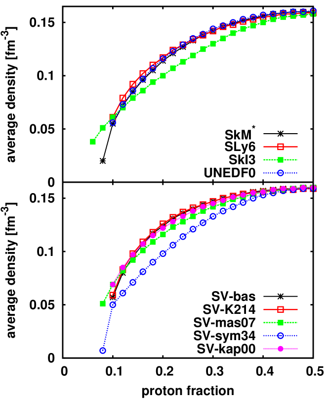
Figure 2: (Color online) Equilibrium density as function of proton fraction $X_{p}$ for different Skyrme interactions (explanations see text). Each curve stops at some low $X_{p}$ because no equilibrium (minimum of energy as function of $\rho$) could be found for smaller $X_{p}$.

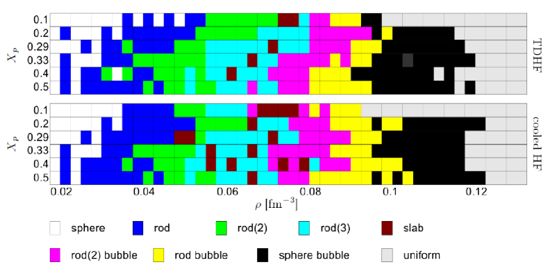
Figure 3: (Color online) Upper panel: Map of pasta shapes achieved in TDHF calculations starting from a gas of $\alpha$-particles with neutron background for various proton fractions and mean densities. Starting from these final states, the map of pasta shapes achieved in Hartree-Fock calculations (cooled pasta) is shown in the lower panel. Two different colors in a cell mark different final states for two calculations with similar initial conditions. The structures are named like in Schuetrumpf et al. (2013) and examples and further properties can be found there.

III.1 Equation of state of homogeneous matter

As a first step, we look at the binding energy curves of homogeneous asymmetric nuclear matter for the SLy6 interaction as shown in Fig. 1. Pure neutron matter ($X_{p}=0$) is unbound, a feature which is well known. Unbound matter persists for small $X_{p}$ up to about $X_{p}=0.09$. For $X_{p}=0.1$ we are able to find a local minimum at non-zero density which, however, is a metastable state. A well bound ground state (negative energy) emerges then from $X_{p}=0.13$ on. Binding and equilibrium densities increase very quickly above $X_{p}=0.13$. We thus have a clear distinction between low proton content $X_{p}$ and moderate or large one with a proton fraction around a critical point $X_{p}\approx 0.13$. Once substantial binding sets on above the critical point, the equilibrium densities saturate quickly around $\rho_{\mathrm{nm}}=0.12-0.16$ fm^-3. Just recently a study appeared of the equation-of-state of asymmetric nuclear matter based on classical molecular dynamics simulations López et al. (2014). Although the formal framework is very different, the classical results at temperatures as low as 2 MeV show the same trends as seen here at zero temperature, e.g., the shape of the binding curves and the drift of the equilibrium density with $X_{p}$.

The sequence of equations of state for different $X_{p}$ looks very similar for all Skyrme interactions which we have studied. It can be characterized by the sequence of equilibrium points shown as black boxes in Fig. 1. Fig. 2 shows this sequence of equilibrium points for a great variety of Skyrme interactions. The upper panel shows results for widely used interactions found in the literature, SkM* Bartel et al. (1982), SLy6 Chabanat et al. (1998), SkI3 Reinhard and Flocard (1995), and UNEDF0 Kortelainen et al. (2010). The lower panel shows results from a set of interactions in which nuclear matter properties have been systematically varied with respect to standard values set in SV-bas Klüpfel et al. (2009), SV-mas07 with lower effective mass, SV-K218 with smaller incompressibility, SV-sym34 with larger symmetry energy, and SV-kap00 with smaller Thomas-Reiche-Kuhn sum rule enhancement factor (equivalent to isovector effective mass). All of the interactions show very similar behavior. The largest deviations are seen for the interactions with untypically large symmetry energy, SkI3 in the upper panel and SV-sym34 in the lower one. Even including these, all interactions show the same trends and the binding energies in dependence on the proton fraction are almost identical. Therefore we expect the results in this work obtained with SLy6 representative for all reasonable Skyrme interactions. Varying the interaction may shift slightly the borders between phases. But the overall sequence should be robust.

III.2 The map of pasta shapes

The map of pasta shapes obtained from the dynamical simulations under various initial conditions is shown in the upper panel of Fig. 3. For every value of $X_{p}$ and mean density $\rho$, two calculations with different initial conditions are performed. These yield in most cases the same phase. There are few cases where two different final states are reached. This is indicated by showing two different colors in a cell. The value $X_{p}=0.3$ is replaced by $X_{p}=1/3$ to establish contact with the previous study Schuetrumpf et al. (2013) which worked exclusively at this proton fraction. To fill the resulting larger gap towards $X_{p}=0.2$, we also show a lower value $X_{p}=0.29$. At first glance, one sees a jump between $X_{p}=0.1$ and the larger $X_{p}$ to the extent that $X_{p}=0.1$ has a much larger range of pure nuclear matter on the side of high $\rho$. This reflects the “phase transition” around $X_{p}\approx 0.13$ observed in the equation of state in Fig. 1. The transition between pure nuclear matter and structured matter is, in fact, predominantly a competition between the spherical bubbles (black boxes) and homogeneous matter. All other shapes show steady, often moderate, changes with $X_{p}$. The sequence in which the shapes appear and disappear with increasing density is practically the same at all $X_{p}$. There is a slight trend, however, that for an increasing proton fraction the different pasta shapes appear at lower mean densities. Take, e.g. the border between rod and rod(2): it is above a mean density of $\rho=0.05{\rm\,fm^{-3}}$ for $X_{p}=0.1$ and moves to about $0.04{\rm\,fm^{-3}}$ for symmetric matter ($X_{p}=0.5$).

In Ref. Okamoto et al. (2013) the trend that for low proton fractions pasta matter appears in a smaller range in density is also clearly visible. The densities for the transitions between normal nuclei, pasta matter, and uniform nuclear matter are in detail different, like in other approaches. These numbers seem to be very sensitive to the equation of state used for the calculations.

It is interesting to compare the present results at $X_{p}=0.33$ to our earlier simulations Schuetrumpf et al. (2013). The sequence of shapes is the same. But the middle region shows more slab configurations. This is probably an effect of different initialization. The earlier calculation allowed a smaller minimal distance between the $\alpha$-particles leading to an initial state which contains more clustered $\alpha$-particles obviously driving the slab phase. The appearance of shapes thus seems to depend to some extent on the initial state. This indicates that the barriers between the different shapes are sufficiently high to stabilize a shape even though it is not necessarily the minimum configuration.

As a further check of the stability of the dynamical configurations, we have cooled each of them down to temperature zero actually starting the static iteration from the final stage of dynamical evolution. The resulting map of shapes is shown in the lower panel of Fig. 3. Most of the dynamical configurations persist when cooled down. There are only a few small shifts of borders between shapes and, not surprisingly, a few more slabs pop up which corrects somewhat the underestimation of slabs.

A subtle difference in detail ought to be mentioned. The border to uniform nuclear matter is shifted to smaller mean densities for $X_{p}=0.1$ but to higher mean densities for all higher proton fractions $X_{p}>0.1$. The jump in the border between uniform nuclear matter and spherical bubbles thus becomes even more pronounced. In fact, the larger jump for the cooled configurations is closer to the sharp transition indicated in the equation of state, see Fig. 1. Increasing temperature weakens this transition.

III.3 Neutron background

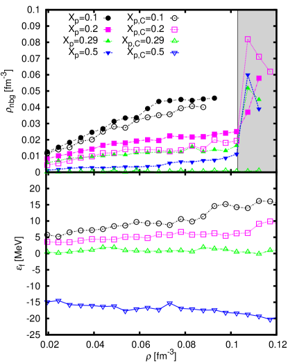
Figure 4: (Color online) Upper panel: Neutron background densities ($\rho_{\rm nbg}$) of the series of calculations of Fig. 3. Full symbols show results from dynamical calculations and open symbols from zero-temperature configurations, marked with the additional index C in the legend. The case $X_{p,C}=0.5$ is not shown because it did not produce a background. The shaded area indicates the region where $\rho_{g}$ is only vaguely defined. Lower panel: Neutron Fermi energies for the cooled Pasta shapes in dependence on the mean density for different proton fractions are shown.

We have matter with very different neutron contents. It is thus interesting to look for the gaseous neutron background density $\rho_{g}$ under the different conditions. In order to find $\rho_{g}$, we follow the strategy of Ref. Schuetrumpf et al. (2013) and compute the distribution of volumes of the neutron density, $v(\rho_{\mathrm{ref}})=\int d^{3}r\,\delta(\rho_{\mathrm{ref}}-\rho_{n}(\mathbf{r}))$. This displays typically a clear peak at low $\rho_{\mathrm{ref}}$. A Gauss fit to this low density peak in the neutron distribution then yields $\rho_{g}$. No clear peak is visible for higher mean densities. In this case, the edge where the curves starts to differ from zero was taken as an indicator. The proton background densities, if present at all, are very small and can be ignored. The results are shown in the upper panel of Fig. 4. The shaded area at high $\rho$ indicates the region where the determination of $\rho_{g}$ becomes uncertain. Naturally, $\rho_{g}$ is very large for the smallest proton fraction $X_{p}=0.1$ and drops quickly with increasing $X_{p}$. The values from cooled configurations are systematically lower than for the dynamical ones. This reflects the fact that cold bound systems can accommodate more extra neutrons than hot ones. For $\rho\gtrsim 0.1{\rm\,fm^{-3}}$ (shaded area) the tails of the density distributions in the voids of the rod bubble or the sphere bubble cover very little space and thus do not reach small values for the density. Therefore in these configurations a large neutron background is present.

While the neutron background is present for all proton fractions in the finite temperature calculations, it vanishes completely for $X_{p}>0.29$ for the zero temperature calculations. In order to corroborate this result, we show in the lower panel of Fig. 4 the neutron Fermi energies $\epsilon_{F,n}$ for the cooled configurations. For $X_{p}=0.1$ and $X_{p}=0.2$, the $\epsilon_{F,n}$ stay significantly above zero, confirming that a large amount of neutrons are unbound. The case of $X_{p}=0.29$ is transitional to the extent that the $\epsilon_{F,n}$ are close to zero and therefore, the neutron background is only marginally present. For $X_{p}=0.33$ the Fermi energies are slightly below zero and thus there is no neutron background present any more. For even higher $X_{p}$ the Fermi energies drop further below zero and yield a strongly bound system. For finite temperature calculations the distribution around the Fermi edge is softened and therefore a small neutron background is present even for large proton fractions.

III.4 Liquid phase

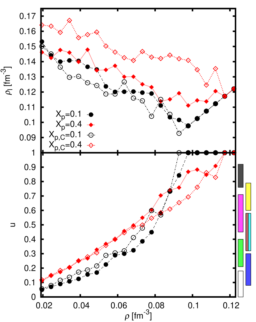
Figure 5: (Color online) Upper panel: Liquid phase densities for two representative values of $X_{p}$. The cooled calculations are marked with the additional index C. Lower panel: Liquid phase occupied volume fractions $u_{l}$ for two $X_{p}$. The color bars on the right indicate a pasta shape with the color code as explained in Fig. 3. The bars mark the intervals of $u_{l}$ for which the pasta shape associated with this color appears.

The liquid densities $\rho_{l}$ are also computed from the distribution of the total density $v(\rho_{\mathrm{ref}})$, but now fitting the high density peaks or flanks. The results for $\rho_{l}$ are shown in the upper panel of Fig. 5. Only graphs for two values of $X_{p}$ are shown because there is very little variation of the $\rho_{l}$ for $X_{p}=0.2...0.5$. The line for $X_{p}=0.4$ is taken to represent all lines for $X_{p}\geq 0.2$. Visibly different is the case $X_{p}=0.1$ where $\rho_{l}$ is lower than for the other $X_{p}$ for both cases, cooled and dynamic. This complies well with the equilibrium densities shown in Fig. 1 which also shows this marked difference between low $X_{p}\leq 0.1$ and larger $X_{p}>0.13$. The actual values for $\rho_{l}$ can differ from the case of homogeneous matter, because the liquid phase is not as neutron rich as the proton fraction indicates due to the separate neutron background and due to surface and Coulomb effects. The liquid phase density decreases with increasing mean density and converges to the mean density below nuclear saturation density. Not surprisingly, the cooled calculations show higher liquid densities because they are better bound. The effect is much more pronounced for high $X_{p}$.

From $\rho_{l}$ and $\rho_{g}\approx\rho_{\rm nbg}$ the volume fraction $u_{l}$ can be derived using Eq. (5). The result is displayed in the lower panel of Fig. 5. Again, we take one representative $X_{p}=0.4$ for the whole group $X_{p}\geq 0.2$. Most curves show an increasing slope, so they grow faster than linearly. This correlates to the fact that the liquid density decreases with increasing density (upper panel of Fig. 5) which results in a larger volume fraction. Very interesting is the behavior of the curves for $X_{p}=0.1$. There are two counteracting effects. First, we have a low liquid density which results in a larger volume fraction. Second, $\rho_{g}$ is very large which reduces the volume fraction. The figure shows that for low mean densities the background neutron effect dominates, resulting in lower volume fraction than for the other $X_{p}$. For higher mean densities the small values for $\rho_{l}$ dominate and the $u_{l}$ for $X_{p}=0.1$ crosses the other lines making the transition from low $u_{l}$ to high ones significantly steeper than for the larger $X_{p}$. This can also be seen in Fig. 3: The sequence of non-trivial shapes (rod until spherical-bubble) is compressed to a smaller range of $\rho$ than for $X_{p}\geq 0.2$.

The impact of the type of the Skyrme force on these results can be estimated from Fig. 2. The main difference is that the liquid densities would be different especially for SkI3 and $a_{\rm sym}=34{\rm\,MeV}$. Therefore the values in Eq. 5 change slightly and the transition points from one to another pasta structure would change. The overall structure of the map of pasta should be the same for all interactions.

IV Conclusion

Using time-dependent Hartree-Fock simulations and static Hartree-Fock calculations, we have investigated the scenarios of the various “pasta” configurations in nuclear matter under astrophysical conditions. Thereby, we have explored the appearance of the different shapes (sphere, rod, slab, …, bubble) in dependence on a given mean density and proton fraction. The dynamical simulations produce thermal states with temperatures in the range 2–7 MeV. The static calculations start from the thermal states and serve to check the stability of geometry under changing thermal conditions.

We find a clear distinction between a regime of low proton fractions $X_{p}\leq 0.13$ and high ones. The results for $X_{p}=0.2...0.5$ show practically the same shapes as function of mean density $\rho$ while the sequence of non-trivial geometries is compressed to a smaller density range for $X_{p}=0.1$. The sequence as such is similar in all cases, starting from isolated spheres (nuclei) at very low density, proceeding over rods, planar meshes of orthogonal rods, triaxial meshes of rods, slabs, to the reciprocal profiles of planar meshes of rod-like bubbles, linear bubble-rods, spherical bubbles, and finally homogeneous matter. The special properties of the small low-density regime are corroborated from the equation of state of homogeneous matter. Matter is unbound for low $X_{p}$. Binding sets on at around $X_{p}=0.13$ and develops very quickly to strong binding with an almost constant equilibrium density.

Generally, the matter segregates into high-density regions of nuclear quantum liquid and low-density regions of a gas of background nucleons, predominantly neutrons. Its density increases with mean density $\rho$ and decreases with increasing $X_{p}$. There is also a significant differences between thermal and cooled state to the extent that the cooled state contains much less neutron gas, for $X_{p}>0.29$ even no gas at all. These observations are corroborated by the neutron Fermi energies which are above zero in the cases of largest neutron gas background.

The volume fraction $u_{l}$ (liquid volume divided by total volume) is the most important parameter determining the pasta shapes. Each shape is found to have a certain interval of $u_{l}$ for which it can appear. The trend $u_{l}(\rho)$ shows also a clear distinction between $X_{p}=0.1$ and all larger $X_{p}$. The curve is steeper for the low $X_{p}$ which is related to the compressed sequence of shapes at $X_{p}=0.1$.

All in all, the results are rather robust in the region of larger proton fraction $X_{p}=0.2...0.5$. This means earlier investigations done for one proton fraction, mostly $X_{p}=1/3$ apply in this whole range. The region of low proton fractions is different and generally more sensitive to the system parameters.