Lagrangian Coherent Structures from Video Streams of Jupiter

1 Introduction

Jupiter’s fast rotation - one rotation over 10 hours - creates strong jet streams, smearing its clouds into linear bands of dark and light zonal belts that circle the planet on lines of almost constant latitude. Such a high degree of axisymmetry is absent in our own atmosphere. Moreover, Jupiter has the largest and longest-living known atmospheric vortex, the Great Red Spot (GRS). Such vortices abound in nature, but GRS’s size, long-term persistence, and temporal longitudinal oscillations make it unique.

Here, we uncover, for the first time, unsteady material structures that form the cores of zonal jets and the boundary of the GRS in Jupiter’s atmosphere. We perform our analysis on a velocity field extracted from a video footage acquired by the NASA Cassini spacecraft.

2 Background: Lagrangian coherent structures

Consider a two-dimensional unsteady velocity field

$$\dot{x}=v(x,t),\quad x\in U\subset\mathbb{R}^{2},\quad t\in[t_{0},t],$$ (1)

which defines a two-dimensional flow over the finite time interval $[t_{0},t]$ in the spatial domain $U$. The flow map $F_{t_{0}}^{t}(x_{0}):x_{0}\mapsto x_{t}$ of (1) then maps the initial condition $x_{0}$ at time $t_{0}$ to its evolved position $x_{t}$ at time $t$. The Cauchy–Green (CG) strain tensor associated with (1) is defined as

$$C_{t_{0}}^{t}(x_{0})={DF_{t_{0}}^{t}}^{\intercal}DF_{t_{0}}^{t},$$ (2)

where $DF_{t_{0}}^{t}$ denotes the gradient of the flow map, and the symbol $\intercal$ indicates matrix transposition. The CG strain tensor is symmetric and positive definite, thus has two positive eigenvalues $0<\lambda_{1}\leq\lambda_{2}$ and an orthonormal eigenbasis $\left\{\xi_{1},\xi_{2}\right\}$, defined as

$$C_{t_{0}}^{t}(x_{0})\xi_{i}(x_{0})=\lambda_{i}(x_{0})\mathbf{\xi}_{i}(x_{0}),\quad\left|\xi_{i}(x_{0})\right|=1,\quad i\in\{1,2\},$$ (3)

We shall suppress the dependence of CG invariants on $t_{0}$ and $t$ for notational simplicity.
A general material line (composed of an evolving curve of initial conditions) experiences both shear and strain in its deformation. As argued in [1, 2], the averaged straining and shearing experienced within a strip of $\epsilon$-close material lines will generally differ by an $\mathcal{O\left(\epsilon\right)}$ amount over a finite time interval due to the continuity of the finite-time flow map.
We seek a Lagrangian Coherent Structure (LCS) as an exceptional material line around which $\mathcal{O\left(\epsilon\right)}$ material belts show no $\mathcal{O\left(\epsilon\right)}$ variation in the length-averaged Lagrangian shear or strain over the time interval $[t_{0},t]$. This implies that an LCS is a stationary curve for the averaged Lagrangian shear or strain functionals.

2.1 Shearless LCSs: stationary curves of averaged shear

Specifically, a shearless LCS is a material line whose averaged shear shows no leading order variation with respect to the normal distance from the LCS. Farazmand et al. [1] show that such curves are null-geodesics of a Lorentzian metric. The most robust class of these null-geodesics turns out to be composed of smooth chains of tensorlines (trajectories of the eigenvector fields of CG) that connect singularities of the CG field. Out of all such possible chains, one builds parabolic LCSs (generalized jet cores) by identifying tensorlines closest to being neutrally stable (cf. Farazmand et al. (2014) for details).

2.2 Strainless LCSs: stationary curves of averaged strain

Similarly, a strainless LCS is a material line whose averaged strain shows no leading order variation with respect to the normal distance from the LCS. As shown by Haller and Beron–Vera [2], such stationary curves of the tangential stretching functional coincide with the null-geodesics of another Lorentzian metric that are tangent to one of the vector fields

$$\eta_{\lambda}^{\pm}(x_{0})=\sqrt{\frac{\lambda_{2}(x_{0})-\lambda^{2}}{\lambda_{2}(x_{0})-\lambda_{1}(x_{0})}}\xi_{1}(x_{0})\pm\sqrt{\frac{\lambda^{2}-\lambda_{1}(x_{0})}{\lambda_{2}(x_{0})-\lambda_{1}(x_{0})}}\xi_{2}(x_{0}),$$ (4)

We refer to the closed orbits (limit cycles) of the vector fields (4) as elliptic LCS. The outermost orbit of such a family of limit cycles serves as a coherent Lagrangian vortex boundary. It is infinitesimally uniformly stretching, i.e., any of its subsets stretches exactly by a factor of $\lambda$ over the time interval $[t_{0},t]$. Limit cycles of $\eta_{\lambda}^{\pm}(x_{0})$ only tend to exist for $\lambda\approx 1$, guaranteeing a high degree of material coherence for the Lagrangian vortex boundary.

3 Results

We used the ACCIV algorithm of Asay-Davis et al. [3] to extract a time-resolved atmospheric velocity field from video footage taken by the NASA Cassini Orbiter. The ACCIV algorithm yields a high density of wind velocity vectors, which is advantageous over the limited number of vectors traditionally obtained from manual cloud tracking.
Observational records of Jupiter go back to the late 19th century, indicating that Jupiter’s atmosphere is highly stable in the latitudinal direction. Therefore, the average zonal velocity profile as a function of latitudinal degree is an important benchmark for examining the quality of the reconstructed velocity field.

In Fig. 1a, we compare our temporally averaged zonal velocity profile obtained form ACCIV algorithm with the profile reported by Limaye [4]. Limaye’s profile is based on Voyager I and Voyager II images, covering 144 Jovian days. Our velocity profile is based on video footage captured by Cassini Orbiter during its flyby in route to Saturn in 2000, just covering 24 Jovian days. Despite these differences in the data, the two profiles show sufficiently close agreement.
Using the extracted time-resolved velocity, we applied the geodesic theory of LCSs reviewed in Section 2 to the detection of a coherent Lagrangian boundary for the GRS, and of the cores of eastward- and westward-moving zonal jets (Fig. 1b). Advected images (not shown here) of the extracted LCSs confirm their sustained coherence and organizing role in cloud transport and mixing. We will report further details and results elsewhere.

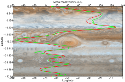
(a)

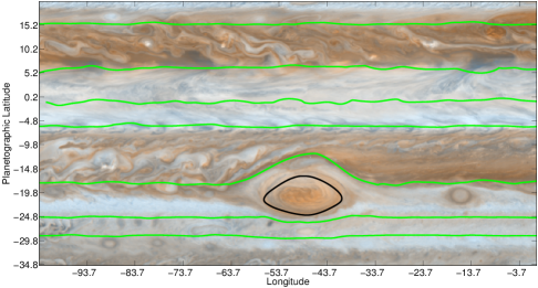
(b)

Figure 1: (A) Zonal velocity profile of Jupiter’s atmosphere. The red line is our velocity profile which is obtained from Cassini images, and the green profile is the velocity profile reported by S.S. Limaye [4]. (B) Shearless LCS (green) as zonal jet cores, and an elliptic LCS (black) as the Lagrangian boundary of the Great Red Spot. (Background image credit: NASA/JPL-Caltech)

References

- [1] Farazmand, M., Blazevski, D, and Haller, G. (2014). Shearless transport barriers in unsteady two-dimensional flows and maps, Physica D, submitted.
- [2] Haller, G. and F. J. Beron-Vera (2013). Coherent Lagrangian vortices: the black holes of turbulence. J. of Fluid Mech. 731. R4
- [3] Asay–Davis, XS., Marcus, P.S., Wonga, M.H., and de Patera, I. (2009). Jupiter’s shrinking Great Red Spot and steady Oval BA: Velocity measurements with the ’Advection Corrected Correlation Image Velocimetry’ automated cloud-tracking method. Icarus 203(1): 164-188.
- [4] Limaye, S. S. (1986). Jupiter - New estimates of the mean zonal flow at the cloud level. Icarus 65(2-3): 335-352.