Spin Excitation Spectra of Spin-Orbit Coupled Bosons in Optical Lattice

Abstract

Spin-wave excitation plays important roles in the investigation of the magnetic phases. In this paper, we study the spin-wave excitation spectra of two-component Bose gases with spin-orbit coupling on a deep square optical lattice using spin-wave theory. We find that, while the excitation spectrum of the vortex crystal phase is gapless with a linear dispersion in the vicinity of the minimum point, the spectra of the commensurate spiral spin phase and the skyrmion crystal phase are gapped. Significantly, the spin fluctuations strongly destabilize the classical ground state of the skyrmion phase. It suggests the emergence of a new state in the phase diagram. Such features of the spin excitation spectra provide further insights into the exploration of the exotic spin phases.

I INTRODUCTION

Typical spin-orbit coupling (SOC) of electrons in solid state system is due to relativistic effect. For instance, it can be derived from the Dirac equation of fermions by expansion in terms of the small parameter $v/c\approx 0.01$, which is the ratio of electron and light speeds in solids. Therefore, the spin-orbit interaction is much weaker than the Coulomb interaction and is generally neglected in the study of condensed matter physics. However, it has been recently noticed that the SOC plays a crucial role in leading to the so-called topological insulating states in solids Hasan ; Qi . Consequently, it attracts many physicists’ attention. In particular, with successful realization of the synthetic gauge field in ultracold quantum gases Lin1 ; Lin2 ; Zhang1 ; Wang1 ; Cheuk , it has been discovered that the spin-orbit coupling may be also important in determining the properties of these systems Wang2 ; Ho ; XuZF1 ; CongjunWu ; Zhang ; Li ; Sinha ; Hu1 ; Wilson ; Kawakami ; Su ; Deng ; Stanescu ; Vyasanakere ; Hu2 ; Yu ; Gong . For example, SOC can produce various new types of ground states such as the stripes, the half-vortex phases in the Bose-Einstein condensates, and a bounded state, which is called Rashbon in the Fermi gases XFZhou ; NGoldman ; HZhai . That makes research on SOC in ultracold gases vigorous.

In addition, ultracold gases on optical lattices have attracted great interests to simulate a wide range of condensed-matter phenomena Lewenstein , such as the the Mott metal-insulator transition and the effects of strong correlation in the Hubbard model Esslinger . As is known, at half filling, the low energy physics of these systems can be indeed described by an effective antiferromagnetic spin Hamiltonian in the deep Mott regime Anderson ; Datta ; Wang3 ; Ji . Therefore, the ground states are generally Neel ordered and the corresponding low-lying excitations are antiferromagnetic magnons.

Then, a natural question which one would like to ask is what effects will be induced if SOC exists in ultracold gases loaded in optical lattice. Actually, in this case, one can derive an additional Dzyaloshinskii-Moriya (DM) type of super-exchange interaction in the deep Mott insulating regime by the second-order perturbation theory Dzyaloshinsky ; Moriya . Very recently, many authors analyzed the phase diagram of this system Cole ; Radic ; Cai ; MGong ; YQian . By applying the classical Monte-Carlo simulations, several exotic spin-textures, whose existences were previously explored in various solid state materials with the DM interaction Pesin ; Heinze ; Banerjee , are also found in ultracold gases.

However, these investigations are not complete from the theoretical point of view. Indeed, up to now, only the classical ground-state phase diagram of the bosonic super-exchange Hamiltonian on a square lattice was numerically explored. But, the effects of spin fluctuations on the stabilities of exotic spin-textures in these phases have been not discussed yet. As is well known, strong spin fluctuations in low-dimensional systems can qualitatively change their phase diagrams outlined by the classical simulations. Therefore, one has to take these fluctuations into consideration in order to determine the stability of each possible phase. In the following, we shall proceed to calculate the low-lying spectra of spin fluctuations in these phases. As a result, we are able to determine the parameter region in which each corresponding phase is stable against spin fluctuations.

Technically, we implement the spin-wave theory developed in Ref. Kleine to derive the global magnetic phase diagram of the super-exchange Hamiltonian. In particular, we calculate the spin-wave excitation spectra for the $XY$-ferromagnet phase, the spiral spin phase and the spin vortex phase, whose existences were studied by the previous classical Monte Carlo simulations Pesin ; Heinze ; Banerjee . We discuss also the stability of a novel phase, the so-called skyrmion crystal phase in bosonic ultracold gases. We show that the possible existing regions for the skyrmion crystal phase are greatly shrunk by the spin fluctuations. More precisely, we find that the spin excitation spectrum of the commensurate spiral spin phase has two minima, which are symmetrical with respect to the $k_{y}$-axis in momentum space. In addition, it possesses a gap, too. On the other hand, the spectrum of the $3\times 3$ skyrmion crystal phase presents some intriguing features, which render its existence fragile. These characteristic excitation spectra may be investigated in the future experiment. Given that the above exotic spin configurations have also been discovered and attracted great interests in recent solid state materials Pesin ; Heinze ; Banerjee ,such features of the spin excitation spectra, which should be observable via the neutron scattering experiments, provide insights into these spin phases.

This paper is organized as follows. In section II, we derive the effective super-exchange spin model for the systems of bosonic gases on a square optical lattice; In section III, we present the general formalism of the spin wave theory developed in Ref. Kleine ; Then, in section IV, we analyze the phase diagram and excitation spectrum of each above-mentioned phase in detail; Finally, in section V, we summarize our main results and discuss some related issues with experiments.

II THE EFFECTIVE SPIN MODEL

Let us consider a boson gas loaded in a two dimensional square optical lattice. The atoms are characterized by two nearly-degenerate states, which are produced by a hyper-fine interaction. In the following, for convenience, we shall use the language of (pseudo)-spin to describe the local occupancy of these states by particles. Furthermore, we take the synthetic spin-orbit interaction into consideration. Then, the Hamiltonian of the bosonic gas can be written as

$$H=-t\sum_{\langle i,j\rangle}(\psi^{\dagger}_{i}\mathcal{R}_{ij}\psi_{j}+{\rm h.c.})+\frac{1}{2}\sum_{i\sigma\sigma^{\prime}}U_{\sigma\sigma^{\prime}}a^{\dagger}_{i\sigma}a^{\dagger}_{i\sigma^{\prime}}a_{i\sigma^{\prime}}a_{i\sigma}.$$ (1)

Here $a_{i\sigma}$ ($a^{\dagger}_{i\sigma}$) denotes boson annihilation (creation) operator, which annihilates (creates) a boson of (pseudo)-spin $\sigma=\uparrow,\downarrow$ at lattice site $i$. In a compact form, these operators can be re-written as $\psi^{\dagger}_{i}\equiv(a^{\dagger}_{i\uparrow},a^{\dagger}_{i\downarrow})$ and its Hermitian conjugate $\psi_{i}$. The first term of $H$ describes the hopping process of bosons between a pair of nearest-neighbor lattice sites $i$ and $j$. The corresponding hopping matrices are given by $\mathcal{R}_{ij}\equiv\exp[i\vec{A}\cdot(\vec{r}_{i}-\vec{r}_{j})]$, where $\vec{A}=(\alpha\sigma_{y},\beta\sigma_{x},0)$ is a non-Abelian gauge field with $\sigma_{x}$ and $\sigma_{y}$ being the Pauli matrices Cole ; Radic ; Goldman . In fact, if we let $\beta=-\alpha$, then $\vec{A}=(\alpha\sigma_{y},-\alpha\sigma_{x},0)$ is the gauge field giving rise to the well-known Rashba SOC. We see that the diagonal part of the hopping matrices $\mathcal{R}_{ij}$ represents the spin-conserved tunneling, while the off-diagonal part is for the spin-flipped tunneling of bosons between the lattice sites $i$ and $j$. Furthermore, the second term in the Hamiltonian stands for the contact interaction between bosons. In general, the intra-species interaction strengths can be different. However we assume them to be equal in the following discussions. More precisely, we set $U_{\uparrow\uparrow}=U_{\downarrow\downarrow}=U$. Similarly, we choose the inter-species interaction $U_{\uparrow\downarrow}=U_{\downarrow\uparrow}\equiv\lambda{U}$ with $\lambda>0$ being a dimensionless parameter.

As is well known, the filling factor of bosons is also an important parameter to determine the properties of ultracold gases on an optical lattice. In the following, we shall only consider the case of one boson per site on average. Now, we can perform the standard Schrieffer-Wolf transformation $H_{\rm eff}=e^{iS}He^{-iS}$ Hewson to the Hamiltonian in the large-$U$ limit $U_{\sigma\sigma^{\prime}}\gg{t}$. It produces an effective Hamiltonian

$$H_{\rm eff}=\sum_{i,\delta=\hat{x},\hat{y}}\left[\sum_{a=x,y,z}J^{a}_{\delta}{}S^{a}_{i}S^{a}_{i+\delta}+\bm{D}_{\delta}\cdot(\bm{S}_{i}\times\bm{S}_{i+\delta})\right],$$ (2)

which captures the low-energy physics of the original system Duan ; Cole ; Radic . Here, ${\bf S}_{i}=(S^{x}_{i},S^{y}_{i},S^{z}_{i})$ are the spin operators of bosons at lattice site $i$. In terms of the boson operators $a_{i\sigma}$ and $a_{i\sigma}^{\dagger}$, they can be written as $S^{x}_{i}=(a_{i\uparrow}^{\dagger}a_{i\downarrow}+a_{i\downarrow}^{\dagger}a_{i\uparrow})/2$, $S^{y}_{i}=(a_{i\uparrow}^{\dagger}a_{i\downarrow}-a_{i\downarrow}^{\dagger}a_{i\uparrow})/2i$ and $S^{z}_{i}=(n_{i\uparrow}-n_{i\downarrow})/2$. In Eq. (2), the first summation is a Heisenberg type of Hamiltonian and the second summation represents the so-called Dzyaloshinskii-Moriya (DM) superexchange interaction. The corresponding coupling constants are given in TABLE I.

$J^{x}_{\hat{x}}=-\frac{4t^{2}}{\lambda{}V}\cos(2\alpha)$	$J^{x}_{\hat{y}}=-\frac{4t^{2}}{\lambda{}V}$
$J^{y}_{\hat{x}}=-\frac{4t^{2}}{\lambda{}V}$	$J^{y}_{\hat{y}}=-\frac{4t^{2}}{\lambda{}V}\cos(2\alpha)$
$J^{z}_{\hat{x}}=-\frac{4t^{2}}{\lambda{}V}(2\lambda-1)\cos(2\alpha)$	$J^{z}_{\hat{y}}=-\frac{4t^{2}}{\lambda{}V}(2\lambda-1)\cos(2\alpha)$
${\bf D}_{\hat{x}}=\frac{4t^{2}}{V}\sin(2\alpha){\bf e}_{y}$	${\bf D}_{\hat{y}}=-\frac{4t^{2}}{V}\sin(2\alpha){\bf e}_{x}$

Table 1: Exchange couplings $J^{a}_{\delta}$ for the Heisenberg term and $\bm{D}_{\delta}$ for the DM superexchange interaction in the effective Hamiltonian.

We would like to emphasize that these interactions favor qualitatively different types of spin orders. In fact, the Heisenberg Hamiltonian gives either the ferromagnetic or the anti-ferromagnetic ordering, while the DM interaction makes the spiral spin ordering possible. In other words, there exists a competition between them. Consequently, their interplay may drive the system to various exotic phases. In the following, we shall first determine the possible existence of several phases in the system and then, analyze their stabilities by applying the spin-wave theory.

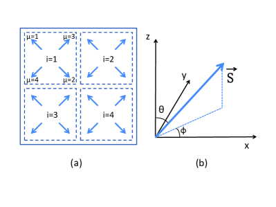
Figure 1: (a) Spin configuration of the $2\times 2$ spin vortex phase, where $i$ denotes the magnetic primitive cell and $\mu$ is the sublattice index. (b) The spin is rotated from the $z$ axis to a new direction ($\theta,\phi$) in the spin-wave theory.

III FORMULISM OF THE SPIN WAVE THEORY

In the previous works, some authors have explored the classical ground states of Hamiltonian (2) by the classical Monte Carlo simulations Cole ; Radic . They showed that the classical ground states of this system support a variety of phases such as the $XY$-ferromagnetic ($XY$-FM) phase, the longitudinal ferromagnetic ($Z$-FM) and antiferromagnetic ($Z$-AFM) phases, the spiral spin phase, the $3\times 3$ skyrmion crystal (SkX) phase, and the $2\times 2$ spin vortex (VX) phase as the coupling constants of Hamiltonian (2) are changed. However, they did not consider the stabilities of these phases. In order to address this issue, one has to take the strong spin fluctuations of the system into consideration, as we do in the following.

To start with, we shall first calculate the ground state energy of each above-mentioned phase in some specified region of parameters by the mean-field theory and see if the previous phase diagram can be re-established. Then, we compute the second-order correction to the energies of those phases. This correction is due to the spin-wave excitations. In some cases, it can render the phase derived by the classical methods invalid. More precisely, as we shall show in the following, the excitation spectrum of a specified phase may develop an imaginary part and hence, becomes a complex function of momentum in some parameter regions. It implies that the assumed phase is actually unstable against the spin fluctuations in these regions. To illustrate the procedure, let us take the $2\times 2$ VX phase for example.

In the first step, we perform the following transformation

$$[S^{x}_{\mu,i},S^{y}_{\mu,i},S^{z}_{\mu,i}]^{T}=\hat{A}_{\mu}[\widetilde{S}^{x}_{\mu,i},\widetilde{S}^{y}_{\mu,i},\widetilde{S}^{z}_{\mu,i}]^{T},$$ (3)

where $i$ denotes the spin primitive cell of the specified phase and $\mu$ is the sublattice index, as shown in Fig. (1a), to $H_{\rm eff}$. The matrix $\hat{A}_{\mu}$ reads

$$\hat{A}_{\mu}=\left(\begin{array}[]{ccc}\cos\theta_{\mu}\cos^{2}\phi_{\mu}+\sin^{2}\phi_{\mu}&\cos\phi_{\mu}\sin\phi_{\mu}(\cos\theta_{\mu}-1)&\sin\theta_{\mu}\cos\phi_{\mu}\\ \cos\phi_{\mu}\sin\phi_{\mu}(\cos\theta_{\mu}-1)&\cos\theta_{\mu}\sin^{2}\phi_{\mu}+\cos^{2}\phi_{\mu}&\sin\theta_{\mu}\sin\phi_{\mu}\\ -\sin\theta_{\mu}\cos\phi_{\mu}&-\sin\theta_{\mu}\sin\phi_{\mu}&\cos\theta_{\mu}\\ \end{array}\right).$$ (4)

It represents the rotation of each spin in the Hamiltonian from the local $z$-axis to a new direction ($\theta,\phi$), as shown in Fig. (1b). Next, we apply Holstein-Primakoff transformation Holstein by substituting the spin operators $\widetilde{S}^{x}_{\mu,i}=(b_{\mu,i}+b^{\dagger}_{\mu,i})/2,\widetilde{S}^{y}_{\mu,i}=(b_{\mu,i}-b^{\dagger}_{\mu,i})/(2i),\widetilde{S}^{z}_{\mu,i}=1/2-b^{\dagger}_{\mu,i}b_{\mu,i}$ into the effective Hamiltonian. Consequently, we obtain $H_{\rm eff}\simeq H_{0}+H_{2}$. Here, $H_{0}$ denotes the mean-field energy for a specific phase and $H_{2}$ is the spin-wave Hamiltonian which describes the spin fluctuation in the system. Let $N$ be the total number of lattice sites, the mean-field energy $H_{0}$ can be written as

$$H_{0} = \frac{N}{16}\sum_{(\mu,\nu)}\left[\cos\phi_{\nu}\sin\theta_{\nu}(-|\bm{D}_{\hat{x}}|\cos\theta_{\mu}+\cos\phi_{\mu}\sin\theta_{\mu}J^{x}_{\hat{x}})+\sin\theta_{\mu}\sin\theta_{\nu}\sin\phi_{\mu}\sin\phi_{\nu}J^{y}_{\hat{x}}\right.$$ (5)

$$+ \left.\cos\theta_{\nu}(|\bm{D}_{\hat{x}}|\cos\phi_{\mu}\sin\theta_{\mu}+\cos\theta_{\mu}J^{z}_{\hat{x}})\right]+\frac{N}{16}\sum_{(\alpha,\beta)}\left[\sin\theta_{\alpha}\sin\phi_{\alpha}(-|\bm{D}_{\hat{y}}|\cos\theta_{\beta}\right.$$

$$+ \left.\sin\theta_{\beta}\sin\phi_{\beta}J^{x}_{\hat{y}})+\cos\phi_{\beta}\cos\psi_{\alpha}\sin\theta_{\beta}\sin\theta_{\alpha}J^{y}_{\hat{y}}+\cos\theta_{\alpha}(|\bm{D}_{\hat{y}}|\sin\theta_{\beta}\sin\phi_{\beta}+\cos\theta_{\beta}J^{z}_{\hat{y}})\right].$$

Here, the spin angles $\theta_{\mu}$ and $\phi_{\mu}$ are determined by the spin configurations of the specified mean-field ground state. For example, in the $2\times 2$ VX phase, we have $\theta_{1}=\theta_{2}=\theta_{3}=\theta_{4}=\pi/2,\phi_{1}=3\pi/4,\phi_{2}=7\pi/4,\phi_{3}=\pi/4$ and $\phi_{4}=5\pi/4$. In addition, $(\mu,\nu)$ and $(\alpha,\beta)$ denote two pairs of nearest-neighbor sites in the primitive cell along the $\hat{x}$- and $\hat{y}$-axis, respectively. With the same notations, we obtain the following spin-wave interaction terms

$$H_{2}=\sum_{\mu}{}M_{\mu\mu}\sum_{i}n_{\mu,i}+\sum_{\mu,\mu^{\prime}}\sum_{<ij>}(M_{\mu,\mu^{\prime}}b^{\dagger}_{\mu,i}b_{\mu^{\prime},j}+N_{\mu,\mu^{\prime}}b^{\dagger}_{\mu,i}b^{\dagger}_{{\mu^{\prime},j}}+{\rm h.c.}),$$ (6)

by keeping only the terms of two-boson operators in the expansion of the transformed effective Hamiltonian. $M_{\mu,\mu^{\prime}}$ and $N_{\mu,\mu^{\prime}}$ are the coefficient matrices depending on the mean-field spin configuration. The explicit expressions of the matrices are tedious and not given here. Then, by using the Fourier transformation, we are able to re-write $H_{2}$ as

$$H_{2}=\frac{1}{2}\sum_{\vec{k}}\beta_{\vec{k}}H_{MN}(\vec{k})\beta^{\dagger}_{\vec{k}}+{\rm const},$$ (7)

where $\beta_{\vec{k}}=(b^{\dagger}_{\vec{k},1},b^{\dagger}_{\vec{k},2},b^{\dagger}_{\vec{k},3},b^{\dagger}_{\vec{k},4},b_{-\vec{k},1},b_{-\vec{k},2},b_{-\vec{k},3},b_{-\vec{k},4})$ are boson operators in the momentum space. Now, we apply the Bogoliubov transformation $\beta_{\vec{k}}=\hat{T}\alpha_{\vec{k}}$ to the effective Hamiltonian $H_{2}$. Due to the bosonic commutation relation, the transformation matrix $\hat{T}$ must be canonical, i.e., relation $\hat{T}^{\dagger}\Lambda\hat{T}=\Lambda$, where

$$\Lambda=\left(\begin{array}[]{cc}1_{4\times 4}&0\\ 0&-1_{4\times 4}\\ \end{array}\right).$$ (8)

should hold true. Furthermore, after substituting the Bogoliubov transformation into Eq. (6), we determine the transformation matrix $\hat{T}$ by requiring that the Hamiltonian be diagonalized by it. In other words, the matrix product $\hat{T}^{\dagger}H_{MN}\hat{T}\equiv\hat{\omega}$ should be a diagonal matrix. With the canonical constraint $\hat{T}^{\dagger}\Lambda\hat{T}=\Lambda$, this condition can be put into an equivalent form

$$(\Lambda\hat{T}\Lambda)^{-1}H_{MN}\Lambda(\Lambda\hat{T}\Lambda)=\hat{\omega}\Lambda.$$ (9)

Consequently, by diagonalizing $H_{MN}\Lambda$ with an invertible matrix $\hat{V}=\Lambda\hat{T}\Lambda$, we can derive the spin excitation spectrum $\omega_{\vec{k},\mu}$ and then, discuss the stability of the $2\times 2$ VX phase by seeing whether the calculated excitation spectral function is complex.

In the following section, we shall study the possible existences and stabilities of the $XY$-FM phase, $Z$-FM phase, $Z$-AFM phases, the spiral spin phase, $3\times 3$ SkX phase, and $2\times 2$ VX phase in ultracold gases on a square optical lattice by the above-outlined procedure. As shown below, although this procedure can be easily applied to most of these phases, it is rather involved for the $3\times 3$ skyrmion crystal phase. The main difficulty is due to the complicated spin configuration of this phase. It contains nine sublattices. In other words, according to the local spin orientations in the $3\times 3$ skyrmion phase, the whole lattice can be divided into nine separate sublattices. In each of them, all the localized spins point in a specified direction. A primitive spin cell of this phase is shown in Fig. 2 (b).

IV ANALYSIS OF THE SPIN EXCITATION SPECTRA

First, we compute the ground-state energy $H_{0}$ for each possible spin configuration listed in the last section and determine the phase diagram by choosing the configuration of the lowest energy in different parameter regions. Then, we shall compare our results with the previous ones derived by the classical Monte Carlo calculations. Our phase diagram is shown by the solid lines in Fig. 2 (a). It is in good agreement with the Monte-Carlo simulations given in Ref. Cole .

Next, we calculate the spin-wave excitation spectrum of each phase and see if it is stable against the spin fluctuations. In fact, we find that the $Z$-AFM and $2\times 2$ VX phases are stable. However, the $3\times 3$ SkX phase is pronouncedly affected by the spin fluctuations. Actually, in two parameter regions, which we paint as white areas in Fig. 2 (a), the spin-wave excitation spectral functions have imaginary parts and hence, render the corresponding phases unstable. On the left side of commensurate 4$\times$1 spiral phase, the unstable parameter region implies the emergence of other commensurate spiral orders or incommensurate spiral phases. While the right unstable parameter region may support new state, which largely suppresses the $3\times 3$ SkX phase.

Now, let us analyze the spin excitation spectrum of each phase in a more detailed manner.

IV.1 $XY$-FM and $Z$-FM Phases

We first consider the weak spin-orbit coupling regime in which the parameter $\alpha$ in TABLE I is small. In this case, the Heisenberg interaction in Hamiltonian (2) is dominant and the DM interaction can be treated as a perturbation. In particular, if we set $\alpha=0$, then the effective Hamiltonian becomes the standard ferromagnetic $XXZ$ model on a two-dimensional square lattice Sachdev . The phase diagram of this model is well known: For $\lambda<1$, all the spins are aligned in the $XY$ plane. More precisely, the system is in the $XY$-FM phase. To this phase, the Holstein-Primakoff transformation can be easily applied.

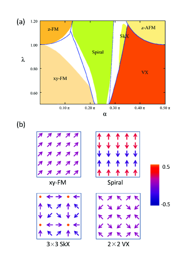
Figure 2: (a) Phase diagram in the Mott insulating regime. The solid lines are the mean-filed results. The filled areas with color are the stable regions, while the white areas are unstable ones under the spin-wave fluctuations. (b) Spin configurations of the $XY$-FM, commensurate 4$\times$1 spiral spin, $3\times 3$ SkX, and $2\times 2$ VX phases.

A direct calculation yields $E(\vec{k})=\sqrt{\frac{1-\lambda}{2}}Ja\sqrt{k_{x}^{2}+k_{y}^{2}}$ for its spin excitation spectrum, in which $J=\frac{4t^{2}}{\lambda{}V}$ and $a$ is the lattice constant. Obviously, the excitation spectrum is gapless with a linear dispersion near $|\vec{k}|\sim 0$, which corresponds to the Goldstone modes in the $XY$-ferromagnets. On the other hand, for $\lambda>1$, the system is in the $Z$-FM phase. The spin excitation spectrum of this phase is given by $E(\vec{k})=\Delta+\frac{Ja^{2}}{4}(k_{x}^{2}+k_{y}^{2})$, which has a spin gap at $\Delta=J(2\lambda-2)$. Finally, $\lambda=1$ is the so-called Heisenberg point at which the model becomes the isotropic Heisenberg ferromagnet. It has a gapless quadratic excitation spectrum, which is shown in Fig. 3.

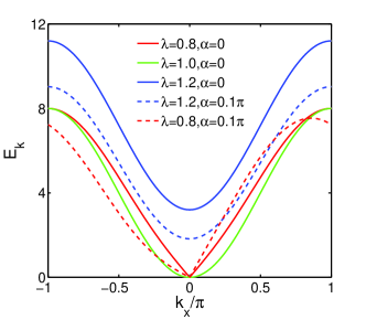
Figure 3: The excitation spectra for the $XY$-FM ($\lambda=0.8$), $Z$-FM ($\lambda=1.5$), and the Heisenberg ferromagnetic ($\lambda=1$) phases. Solid and dashed lines are for the strength of SOC $\alpha=0$ and $\alpha=0.1\pi$, respectively.

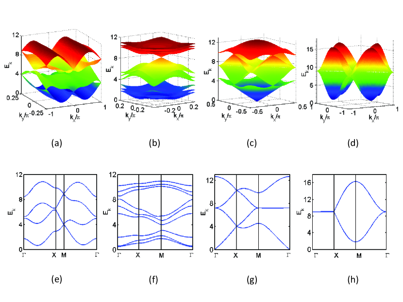
Figure 4: (Color online) The excitation spectra for (a,e) 4$\times$1 spiral spin phase ($\lambda=0.8,\alpha=0.24\pi$). (b,f) 3$\times$3 skyrmion crystal phase ($\lambda=0.9,\alpha=0.32\pi$), (c,g) 2$\times$2 spin vortex phase ($\lambda=0.8,\alpha=0.4\pi$), and (d,h) Z-AFM ($\lambda=1.2,\alpha=0.4\pi$) phases.

Next, we take the effect of the DM interaction into consideration. We find that the excitation spectrum remains still gapless and linear near $|\vec{k}|\sim 0$ for the $XY$-FM phase. But, it becomes asymmetric with respect to $k_{x}=0$ as shown by the dashed line of $\lambda=0.8$ and $\alpha=0.1\pi$ in Fig. 3. Similar dispersion occurs along the $k_{y}$ axis. In the meantime, the gap of the $Z$-FM phase is decreased upon the increasing strength of SOC. However, both the spin excitation spectra of the $XY$-FM and $Z$-FM phases will become imaginary as the SOC strength $\alpha$ is further enhanced. It indicates that these phases are destabilized. This region of parameters is characterized by the white area on the left side of spiral phase in Fig. 2 (a).

IV.2 Spiral Spin Phase

In the middle region of Fig. 2 (a), the DM interaction is strong, comparing with the Heisenberg interaction. The competition between these interactions leads to a spiral spin phase. To determine the stability of this phase, we consider a commensurate 4$\times$1 periodic structure with all the spins lying in the $z-y$ plane. Notice that, in this configuration, the angles $\theta_{i}$ between the spins and $z$ axis are specified by $\theta_{1}=\theta_{2}$, $\theta_{3}=\theta_{4}$, and $\theta_{1}+\theta_{3}=\pi$.

Then, we calculate the excitation spectrum of this phase by the spin-wave analysis. Our results are shown in Fig. 4 (a) and Fig. 4 (e). One can easily see that there exists a spin gap in the diagram. In other words, the Goldstone mode is absent in this phase. Moreover, the gap has two symmetric minima at ($\pm{}k_{0},0$), as shown in Fig. 4 (a). It is due to the fact that the spin configuration in the spiral spin phase is symmetric with respect to the $y$-axis. By varying parameter $\alpha$, we find that the energy gap gradually closes as the DM interaction increases and the excitation spectrum becomes linear in the vicinity of these minimal points. At the same time, the 4$\times$1 periodic structure becomes unstable. It suggests the emergence of of other commensurate spiral orders or incommensurate spiral phases.

IV.3 $2\times 2$ VX and $Z$-AFM Phases

Next, let us consider the large spin-orbit coupling regime around $\alpha=\pi/2$, in which the spin-conserving hopping of particles is suppressed. The Wilson loop, which is characterized by $W={\rm tr}[R_{x}R_{y}R_{x}^{\dagger}R_{y}^{\dagger}]$ is reduced to a marginally abelian one with $|W|=2$ Goldman . In this situation, the Heisenberg interaction is dominant and the spin configuration is determined by a uniform antiferromagnetic interaction in the $Z$-direction plus anisotropic spin-interactions in $X$- and $Y$-directions. When parameter $\lambda<1$, the spin interaction in the $XY$-plane is stronger. Therefore, the system has a co-planar magnetic order. On the other hand, since the spin interaction is antiferromagnetic in the $X$-direction but ferromagnetic in the $Y$-direction, the classical ground state of the system becomes a $2\times 2$ vortex crystal. Further analysis yields the spin-wave spectrum of this phase, as shown in Fig. 4(c) and Fig. 4(g). We find that it has no gap and is linear in the vicinity of the minimum $\Gamma$ point. In contrast, for $\lambda>1$, the system enters the $Z$-AFM phase. Its excitation spectrum is shown in Fig. 4(d) and Fig. 4(h). Now, energy gaps open up at both momenta $(\pm\pi,0)$ and $(0,\pm\pi)$.

IV.4 $3\times 3$ SkX Phase

Finally, we study the $3\times 3$ skyrmion crystal phase, which is located in the phase diagram between the $4\times 1$ spiral spin phase and the $2\times 2$ VX phase. As mentioned at the end section III, The spin configuration of this phase consists of nine sublattices, which are characterized by an up-spin at the center and others lying on the $XY$-plane. By the spin-wave theory, we calculate its spin excitation spectrum. Our results are shown in Fig. 4(b) and Fig. 4(f). Obviously, the spectrum has also an energy gap. Interestingly, we find that the spin fluctuations dramatically destabilize this classical ground state and make the skyrmion crystal phase unstable in part of the classical phase diagram determined by the Monte Carlo simulations Cole . It may imply the appearance of a novel state in the concerned region. However, in order to determine the properties of this state, one must carry on more sophisticated analysis.

V CONCLUSIONS

In summary, we study the exotic magnetic phases of two-component Bose gases with spin-orbit coupling on a deep square optical lattice by using spin-wave theory. In particular, we systematically investiagte the spin-wave excitation spectra for the $XY$-ferromagnet, spiral spin, spin vortex, and skyrmion crystal phases. We find that, while the excitation spectrum of the vortex crystal phase has no gap and is linear in the vicinity of the center of Brillouin zone, the spectra of the commensurate spiral spin phase and the skyrmion crystal phase possess energy gaps. Experimentally, these spin textures can be easily observed through spin-resolved time-of-flight measurements Lin2 . We discuss also the stability of the novel skyrmion crystal phase and show that the possible existing regions for the skyrmion crystal phase are greatly shrunk by the spin-wave excitations. It suggests the emergence of a new state in these regions. Finally, we would like to emphasize that similar spin textures, which are discussed in the present work, can be also induced by the DM type of interactions in some solid state materials. Therefore, we believe that the current investigation should provide with further insights into the study of these materials.

- (1) M. Hasan and C. Kane, Rev. Mod. Phys. 82, 3045 (2010).
- (2) X.-L. Qi and S.-C. Zhang, Rev. Mod. Phys. 83, 1057 (2011).
- (3) Y.-J. Lin, R. L. Compton, K. Jimenez-Garcia, J. V. Porto, and I. B. Spielman, Nature 462, 628 (2009).
- (4) Y.-J. Lin, K. Jiménez-García, and I. B. Spielman, Nature 471, 83 (2011).
- (5) J.-Y. Zhang, S. C. Ji, Z. Chen, L. Zhang, Z. D. Du, B. Yan, G. S. Pan, B. Zhao, Y. J. Deng, H. Zhai, S. Chen, and J. W. Pan, Phys. Rev. Lett. 109, 115301 (2012).
- (6) P.-J. Wang, Z.-Q. Yu, Z.-K. Fu, J. Miao, L.-H. Huang, S.-J. Chai, H. Zhai, and J. Zhang, Phys. Rev. Lett. 109, 095301 (2012).
- (7) L. W. Cheuk, A. T. Sommer, Z. Hadzibabic, T. Yefsah, W. S. Bakr, and M. W. Zwierlein, Phys. Rev. Lett. 109, 095302 (2012).
- (8) T. D. Stanescu, B. Anderson, and V. Galitski, Phys. Rev. A 78, 023616 (2008).
- (9) C. J. Wang, C. Gao, C.-M. Jian, and H. Zhai, Phys. Rev. Lett. 105, 160403 (2010).
- (10) T.-L. Ho and S. Z. Zhang, Phys. Rev. Lett. 107, 150403 (2011).
- (11) Z. F. Xu, R. Lü, and L. You, Phys. Rev. A 83, 053602 (2011).
- (12) C.-J. Wu, I. M. Shem, and X.-F. Zhou, Chin. Phys. Lett. 28, 097102 (2011).
- (13) Y. P. Zhang, L. Mao, and C. W. Zhang, Phys. Rev. Lett. 108, 035302 (2012).
- (14) Y. Li, L. P. Pitaevskii, and S. Stringari, Phys. Rev. Lett. 108, 225301 (2012).
- (15) S. Sinha, R. Nath, and L. Santos, Phys. Rev. Lett. 107, 270401 (2011).
- (16) H. Hu, B. Bamachandhran, H. Pu, and X.-J. Liu, 108, 010402 (2012).
- (17) R. M. Wilson, B. M. Anderson, and C. W. Clark, Phys. Rev. Lett. 111, 185303 (2013).
- (18) T. Kawakami, T. Mizushima, M. Nitta, and K. Machida Phys. Rev. Lett. 109, 015301 (2012).
- (19) S.-W. Su, I.-K. Liu, Y.-C. Tsai, W. M. Liu, and S.-C. Gou, Phys. Rev. A 86, 023601 (2012).
- (20) Y. Deng, J. Cheng, H. Jing, C.-P. Sun, and S. Yi, Phys. Rev. Lett. 108, 125301 (2012).
- (21) J. P. Vyasanakere, S. Zhang, and V. B. Shenoy, Phys. Rev. B 84, 014512 (2011).
- (22) H. Hu, L. Jiang, X.-J. Liu, and H. Pu, Phys. Rev. Lett. 107, 195304 (2011).
- (23) Z.-Q. Yu and H. Zhai, Phys. Rev. Lett. 107, 195305 (2011).
- (24) M. Gong, S. Tewari, and C. Zhang, Phys. Rev. Lett. 107, 195303 (2011).
- (25) X. F. Zhou, Y. Li, Z. Cai, C. J. Wu, J. Phys. B: At. Mol. Opt. Phys. 46, 134001 (2013).
- (26) N. Goldman, G. Juzeliūnas, P. Öhberg, I. B. Spielman, arXiv:1308.6533 (2013).
- (27) H. Zhai, arXiv:1403.8021 (2014).
- (28) M. Lewenstein, A. Sanpera, V. Ahu nger, B. Damski, A. Sen De, and U. Sen, Adv. Phys. 56, 243 (2007).
- (29) T. Esslinger, Annu. Rev. Condens. Matter Phys. 1, 129 (2010).
- (30) P. W. Anderson, Phys. Rev. 115, 2 (1959).
- (31) N. Datta, R. Fernandez, and J. Fröhlich, J. Stat. Phys. 96, 545 (1999).
- (32) Z. J. Wang, and X. M. Qiu, Commun. Theor. Phys. 28, 51 (1997).
- (33) A.-C. Ji, J. Wang, and G.-S. Tian, Commun. Theor. Phys. 37, 607 (2002).
- (34) I. Dzyaloshinsky, J. Phys. Chem. Solids 4, 241 (1958).
- (35) T. Moriya, Phys. Rev. 120, 91 (1960).
- (36) W. S. Cole, S. Z. Zhang, A. Paramekanti, and N. Trivedi, Phys. Rev. Lett. 109, 085302 (2012).
- (37) J. Radi, A. Di Ciolo, K. Sun, and V. Galitski, Phys. Rev. Lett. 109, 085303 (2012).
- (38) Z. Cai, X. Zhou, and C. Wu, Phys. Rev. A 85, 061605(R) (2012).
- (39) M. Gong, Y. Y. Qian, V. W. Scarola, and C. W. Zhang, arXiv:1205.6211 (2012).
- (40) Y. Qian, M. Gong, V. W. Scarola, and C. W. Zhang, arXiv:1312.4011 (2013).
- (41) D. Pesin and L. Balents, Nature phys. 6, 376 (2010).
- (42) S. Heinze, K. von Bergmann, M. Menzel, J. Brede, A. Kubetzka, R. Wiesendanger, G. Bihlmayer, and S. Blügel, Nature phys. 7, 713 (2011).
- (43) S. Banerjee, O. Erten, and M. Randeria, Nature phys. 9, 626 (2013).
- (44) B. Kleine, E. Mller-Hartmann, K. Frahm, and P. Fazekas, Z. Phys. B 87, 103 (1992).
- (45) N. Goldman, A. Kubasiak, A. Bermudez, P. Gaspard, M. Lewenstein, and M. A. Martin-Delgado, Phys. Rev. Lett. 103, 035301 (2009).
- (46) A. C. Hewson, The Kondo Problems to Heavy Fermions (Cambridge University Press, Cambridge, England, 1997).
- (47) L. M. Duan, E. Demler, and M. D. Lukin, Phys. Rev. Lett. 91, 090402 (2003).
- (48) T. Holstein and H. Primakoff, Phys. Rev. 58, 1098 (1940).
- (49) S. Sachdev, Quantum Phase Transitions (Cambridge University Press, 2011).