Power Control for Sum Rate Maximization on Interference Channels Under Sum Power Constraint

Abstract

In this paper, we consider the problem of power control for sum rate maximization on multiple interfering links (TX-RX pairs) under sum power constraint. We consider a single frequency network, where all pairs are operating in same frequency band, thereby creating interference for each other. We study the power allocation problem for sum rate maximization with and without QoS requirements on individual links. When the objective is only sum rate maximization without QoS guarantees, we develop an analytic solution to decide optimal power allocation for two TX-RX pair problem. We also develop a low complexity iterative algorithm for three TX-RX pair problem. For a generic $N>3$ TX-RX pair problem, we develop two low-complexity sub-optimal power allocation algorithms. The first algorithm is based on the idea of making clusters of two or three TX-RX pairs and then leverage the power allocation results obtained for two and three TX-RX pair problems. The second algorithm is developed by using a high SINR approximation and this algorithm can also be implemented in a distributed manner by individual TXs. We then consider the same problem but with additional QoS guarantees for individual links. We again develop an analytic solution for two TX-RX pair problem, and a distributed algorithm for $N>2$ TX-RX pairs.

I Introduction

The aggressive re-use of wireless spectrum (due to spectrum scarcity) in a wireless network can result in several interfering links and a significant degradation in system throughput. Some of the adverse effects of interference can be mitigated through power control and cooperation among transmitters. Power control in different types of wireless networks has been an area of active research for last several years. Recently cooperative communication techniques have also gained a lot of research interest since cooperating transmitters can better manage interference and improve the performance of a wireless network.

With an emerging interest in renewable energy sources and energy harvesting schemes, several new and interesting problems arise in terms of power control in certain wireless and cognitive radio networks. One can imagine a scenario where a battery harvested energy from solar panel, and is providing power to multiple transmitters (sensor nodes, distributed antennas, transmitters in small cells etc). In this situation, the harvested energy in any time slot is shared among multiple transmitters and the resulting optimization problem consists of a sum power constraint on multiple interfering links. The sum power constraint could also provide a fair comparison under certain scenarios in heterogeneous network. This constraint may also arise in games played by resource-constrained players: e.g. in cognitive radio networks and wireless networks. These games are characterized by a central feature that each user has a multi-dimensional action space, subject to a single sum resource constraint. Consideration of power sharing among multiple TXs is also motivated in the emerging scenario of distributed antenna systems (DAS). In DAS, multiple antennas are geographically placed at various locations in the cell. These antennas are connected to a central common source via wired connections [disant_1]. Optimal power allocation among multiple interfering transmitters for sum rate maximization in general is a very challenging problem due to the fact that the capacity region of an interference channel has still not been completely characterized for two or more interfering links [int_chan].

I-A State of the art

A good review of power control techniques in wireless networks can be found in [chiang, rev_n, rev_ref1, rev_ref2]. Several authors have formulated optimization problems for power control in different wireless network settings where interference is not considered or it is treated as part of noise [non_coop1]-[non_coopN]. In most of these papers, the developed optimization problem is converted into a convex optimization problem with zero duality gap. Lagrange dual decomposition techniques are then used to obtain optimal power control which results in water-filling over the inverse of channel gain values [boyd_1]. However, in a practical network where various transmitters are operating in the same frequency band, ignoring interference can be a huge disadvantage in terms of system throughput. Unfortunately, by considering the influence of interference, the resulting power control problem becomes a non-convex optimization problem. Most of existing results show that the power control problems over interfering links are usually NP-hard problems [rev_ref6].

The problem of sum rate maximization for a binary interference link (link and TX-RX pair are used interchangeably throughout the paper) has been considered in [int_cont1]-[int_cont4] under various assumptions (binary interference link means that “TX1 is connected to RX1 and TX2 is connected to RX2 on the same frequency band”). In [int_cont1], [int_cont2], this problem has been studied for the case of strong interference where the message from the strong interferer is decoded first. In [int_cont4], the authors consider the sum rate maximization problem in a symmetric network of interfering links by identifying an underlying convex structure. The authors also allow multiple receivers to coexist in same frequency band. In [kiani_1]-[kiani_n], the authors prove that for binary interfering wireless link, when each link has its own maximum transmit power constraint, the maximum sum rates solution is one of three points: one link transmitting with full power while the other link is silent, or both links transmitting at full power simultaneously. These results are achieved through the analysis of the objective function. In [rev_ref10], the authors analyze the rate region frontiers of $N$ user interference channel while treating interference as noise. They show that the achievable rate region is the convex hull of a union of $N$ rate regions. Each region is outer-bounded by a hyper surface frontier of dimension $N-1$. Using this analysis, the authors in [rev_ref11], show that for binary case, the achievable rate region is a union of two regions and each region is outer-bounded by a log defined line. The authors then analyze the first derivatives of the rate region frontiers and proves the same power control results which are reported in [kiani_1]-[kiani_n] for binary interfering links. In [kk_x], the authors consider the power control problem of two interfering wireless links with individual max power constraints and minimum data rate constraints. The authors prove that in this problem, the optimal solution is again when both links transmit with max power, or when one link transmits with max power and the second transmits with sufficient power which allows it to satisfy its minimum rate constraints. In [rev_ref], the authors consider the sum rate maximization problem for a set of TX-RX pairs operating in a common spectrum band. They optimize the allocation of power spectral densities in Gaussian interference network with flat fading and propose an iterative algorithm for bandwidth and power allocation for multiple users. In [our_globecom], the authors consider optimal power control and optimal antenna selection problem in a multi-user distributed antenna system (only two antennas) connected to a single RF chain under sum-power constraint. The authors develop a low complexity algorithm while ensuring the QoS requirements of delay sensitive users.

There are several works in the literature that also discuss interference management for multiple interfering links. Some popular algorithms in the literature include the interference pricing algorithm [rev_ref3], [rev_ref4] and Weighted Minimum Means Square Error (WMMSE) algorithm [rev_ref5]. In interference pricing algorithms [rev_ref3], [rev_ref4], each link announces an interference price that represents the marginal cost of interference from other links in the network. The links then iteratively update their power and converge to a stationary point, under certain conditions on the utility function (which is being maximized). The set of utility functions unfortunately does not include the standard Shannon rate function. The WMMSE algorithm proposed in [rev_ref5], transforms the weighted sum-rate maximization problem in MIMO broadcast downlink channel to an equivalent weighted sum MSE minimization problem. The proposed algorithm can handle fairly general utility functions and the sequences of iterates produced by the algorithm converges to a local optima with low complexity. Power control problem with linearly coupled constraint (sum power constraint, or more generally interference temperature constraint), is also considered in some recent works [rev_ref8, rev_ref9, linear_coup]. The authors in [rev_ref8] consider a cognitive radio setup, and their objective is to limit the aggregated power of the interference generated by the unlicensed network falls below a certain threshold. They propose a distributed algorithm that converges to a specified set of equilibrium. Using a game theoretical approach, the authors in [rev_ref9] develop algorithms for MIMO cognitive radio network. The proposed algorithms are designed such that they do not violate the interference temperature constraints. In [linear_coup], the authors use game theoretic tools to analyze a broad family of games played by resource-constrained players. These games are characterized by a central feature that each user has a multi-dimensional action space, subject to a single sum resource constraint and each user’s utility in a particular dimension depends on an additive coupling between the user action in the same dimension and the actions of the other users. The authors then explore the properties of these games and provide several sufficient conditions under which best response dynamics converges linearly to the unique NE.

In general, optimal power control for sum rate maximization under individual maximum power constraint per interfering link or sum power constraint for multiple interfering links (with or without QoS guarantees for individual links) remains unknown.

I-B Problem Addressed and motivation

In this paper, we consider the power control problem for sum rate maximization over multiple interfering TX-RX pairs connected to a common energy source. Each RX is assumed to be connected to only one TX. The consideration that all the TXs are connected to a common energy source gives rise to a sum power constraint i.e. there is a constraint on total power budget available for multiple transmitters denoted by $P_{T}$. Moreover, since each TX has access to all the available supply, therefore its transmit power constraint is also equal to $P_{T}$ and the power allocated to any TX $i$ to communicate with its corresponding RX can be any value between $0$ and $P_{T}$. In centralized solution, all the TXs are connected to a centralized node / controller. Power allocation decisions are carried out at the central node based on channel feedback information obtained from various TXs. Power allocation decisions are then communicated to individual TXs which then draw the allocated amount of power from the common energy source. In some cases, we also consider distributed solution, where each TX individually decides its transmit power, and centralized node is not required. Consideration of sum power constraint is mainly motivated in following emerging scenarios:

• Energy harvesting based communication systems: an energy harvester captures green energy from the environment. The harvested energy is used to operate multiple transmitters, e.g. solar panel powered battery which powered multiple transmitters.

• Distributed antenna systems: In DAS, multiple antennas are geographically placed at various locations. These antennas are connected to a common central source via wired connections.

• For fair comparison in heterogeneous networks: e.g. under same sum power constraint, some macro BS traffic being offload to femto BS.

• Games played by resource-constrained players: e.g. in cognitive radio networks and wireless networks. These games are characterized by a central feature that each user has a multi-dimensional action space, subject to a single sum resource constraint.

Furthermore, the solution of sum rate maximization problem under sum power constraint will also provide an upper bound under cooperation in power sharing and power transfer which might become possible in future for some communication systems over short distances.

I-C Contributions

The major contributions of this work are listed below:

• Optimal power control algorithm for two TX-RX pairs without QoS guarantees: We develop an optimal power control for sum rate maximization under sum power constraint for two TX-RX pair problem. The developed solution consists of a very simple criterion to decide between binary or sharing type of power controls. In binary power control, only one TX gets full power while the second TX remains silent. In sharing power control, both the transmitters get non-zero power. In this case, the optimal power allocation to each TX can be determined by solving a simple quadratic equation.

• Low complexity power control algorithm for three TX-RX pairs without QoS guarantees: We develop a low complexity iterative power control algorithm for three TX-RX pair problem. In this algorithm, transmit power of one TX is iteratively updated while the transmit power of remaining two TXs is analytically determined.

• Low Complexity sub-optimal power control algorithms for $N>3$ TX-RX pairs without QoS guarantees: We develop two low complexity sub-optimal algorithms for $N>3$ TX-RX pair problem. The first algorithm is based on clustering technique. The second algorithm is developed by using a high SINR approximation and this algorithm can also be implemented in a distributed manner by individual TXs without the requirement of the central node. The performance evaluation based on the simulated network scenarios in section IV indicate that the clustering algorithm performs well when total available power is less while the distributed algorithm performs well when total available power is high.

• Analytical power control algorithm for two TX-RX pairs with QoS guarantees for individual links: We develop an analytical power control algorithm for sum rate maximization when there are additional requirements of providing QoS guarantees for individual links. The developed solution in this case again comprises of solving simple equations.

• Low Complexity sub-optimal distributed power control algorithm for $N>2$ TX-RX pairs with QoS guarantees for individual links: Using a high SINR approximation, we develop a low complexity sub-optimal power control algorithm. This algorithm provides QoS guarantees for individual links and can be implemented in a distributed manner for any number of TX-RX pairs in the network.

I-D System Model

In this paper, we consider a generic system model consisting of multiple TX-RX pairs located inside a certain geographical area. The TXs are connected (on a wired channel) to a central node. Each RX is assumed to estimate its direct channel gain from its own TX and interference channel gains from other interfering TXs. This information is then communicated to the central node. We assume that the channel gains among TXs and RXs remain constant for the duration of a given time slot but may vary from one time slot to another. The central node as well as all the TXs in the system are powered by a common energy source, e.g. a common battery charged by a solar panel. Power control decisions are made at the central node and these decisions are communicated to corresponding TXs. Based on power allocation decisions, each TX draws the allocated amount of power from the energy source. The system model is shown in Fig. 1.

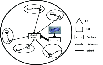
Figure 1: System Model

In the paper we also develop some distributed algorithms. It should be noted that the distributed algorithms can be implemented by individual TXs without the requirement of the central node. We assume that all the TXs are operating in same frequency band and creating interference to each other. The interference channel for five interfering links is depicted in Fig. 2.

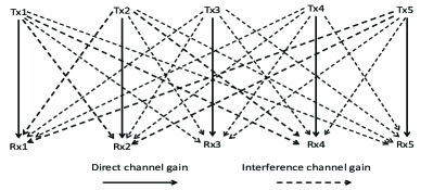
Figure 2: Interference Channel: Five TX-RX pairs

I-E Paper Organization

The rest of the paper is organized as follows. In Section II we formulate the optimization problem without QoS constraints and propose power control algorithms for two, three and $N>3$ TX-RX pairs. In Section LABEL:sec:qos we formulate the optimization problem with QoS constraints for individual links. In this section, we present power control algorithms for two and $N>2$ TX-RX pairs. Simulation results are presented in Section LABEL:sec:sim while the paper is concluded in Section LABEL:sec:conc.

II Power Control Without QoS Constraints

In this section, we formulate the optimization problem and develop power control algorithms when there is no QoS guarantee for individual links. Let $P_{i}$ denote the power allocated to TX $i$ to communicate with its respective RX $i$. Our objective is to make power allocation decisions for sum-rate maximization subject to sum power constraint. We can formulate the following optimization problem:

$$\max_{P_{1},P_{2},...,P_{N}}\>\mathcal{C}(P_{1},P_{2},...,P_{N})$$ (1)

subject to,

$$\sum_{i=1}^{N}P_{i}\leq P_{T}$$ (2)

$$0\leq P_{i}\leq P_{T}\quad\forall i=1,\ldots,N$$ (3)

where $\mathcal{C}(P_{1},P_{2},...,P_{N})$ represents sum-rate function. Constraint (2) is the sum power constraint. This constraint is a linear coupling constraint which indicates that the total power resource is constrained. Constraint (3) are individual power constraints per TX. We assume that each TX can adaptively vary its transmit power depending on the power allocation decisions and the power amplifier is capable to transmit with with any value of $P_{i}$ between $0$ and $P_{T}$. We can use the widely used Shannon’s capacity formula to define the sum-rate function as follows:

$$\mathcal{C}(P_{1},P_{2},...,P_{N}) =\sum_{i=1}^{N}R_{i}(P_{1},P_{2},...P_{N})$$ (4)

$$=\sum_{i=1}^{N}\log_{2}(1+\frac{g_{ii}P_{i}}{\sum_{j\neq i}P_{j}g_{ji}+\sigma^{2}})$$ (5)

In this formulation, $g_{ji}$ denotes the channel gain from TX $j$ to RX $i$ while $\sigma^{2}$ is the Additive White Gaussian Noise (AWGN) noise and $\sum_{j\neq i}P_{j}g_{ji}$ is the interference experienced by TX-RX pair $i$ from all other TXs. The objective function (5) is a non-convex function as can be verified from its Hessian. Due to non-convexity of the problem, it is a difficult problem to solve since convex optimization techniques cannot be applied. Convex optimization has several advantages compared to non-convex or nonlinear optimization techniques. For convex optimization problems; duality gap is zero and any local optimum is also a global optimum of the problem; efficient algorithms can be easily developed [boyd_1]. For non-convex or non-linear optimization problems, meta-heuristics e.g. neighborhood search algorithms, simulated annealing algorithms, genetic algorithms etc. are used. These algorithms converge slowly and can even fail to return a global optimum if fast convergence is required (since local optimum and global optimum are not the same).

II-A Optimal Power Control for two TX-RX pair problem without QoS guarantees

The optimization problem for two TX-RX pairs without QoS guarantees for individual links can be written as,

$$\max_{P_{1},P_{2}}\>\mathcal{C}(P_{1},P_{2})$$ (6)

$$\text{subject to,}\quad P_{1}+P_{2}\leq P_{T}$$ (7)

$$0\leq P_{1}\leq P_{T},\quad\quad 0\leq P_{2}\leq P_{T}$$ (8)

where, $$\mathcal{C}(P_{1},P_{2})$$

$$=\log_{2}(1+\frac{g_{11}P_{1}}{g_{21}P_{2}+\sigma^{2}})+\log_{2}(1+\frac{g_{22}P_{2}}{g_{12}P_{1}+\sigma^{2}})$$

$$=\log_{2}(1+\frac{aP_{1}}{bP_{2}+1})+\log_{2}(1+\frac{dP_{2}}{cP_{1}+1})$$ (9)

Here $a$, $b$, $c$, $d$ are four positive constants: $a=g_{11}/\sigma^{2}$, $d=g_{22}/\sigma^{2}$, $b=g_{21}/\sigma^{2}$ and $c=g_{12}/\sigma^{2}$, where $a$ and $d$ denote the direct channel gains while $b$ and $c$ denote the interference channel gains. It is obvious that the optimal solution to the above optimization problem (6) can result in either binary power control, i.e. $(P_{T},0)$ or $(0,P_{T})$ or sharing power control, i.e. $(0<P_{1}<P_{T},0<P_{2}<P_{T}-P_{1})$. We will now find the conditions under which these solutions are optimal without imposing any restrictions on the channel gain values. Depending on the direct channel gain values, there are two possibilities: $a>d$ or $d>a$.

II-A1 Case: $a>d$

In this case the direct channel gain of TX-RX pair 1 is greater than the direct channel gain of TX-RX pair 2. As a consequence, if binary power allocation scheme turns out to be optimal then all the power should be assigned to TX-RX pair 1. In this case, we can decide the type of power control (binary or power sharing) based on the following simple rule.

Theorem 1.

Compute $\phi=\frac{(a-d)(P_{T}b+1)}{ac+bd-ad+P_{T}abc}$; then depending on the value of $\phi$ decide the type of power control as follows:

1. If $\phi>0$, $(P_{T},0)$ is the optimal solution.

2. If $\phi<0$ and $|\phi|\geq P_{T}$, again $(P_{T},0)$ is the optimal solution.

3. If $\phi<0$ and $|\phi|\leq P_{T}$, there exists a power sharing profile $(0<P_{1}<P_{T},0<P_{2}<P_{T}-P_{1})$ such that $R_{1}(P_{T},0)<R_{1}(P_{1},P_{2})+R_{2}(P_{1},P_{2})$.

$|x|$ denotes the absolute value of $x$.

Proof.

Proof is provided in the conference version of this paper in [our_spawc]. ∎

II-A2 Case: $d>a$

In this case the direct channel gain of TX-RX pair 2 is greater than the direct channel gain of TX-RX pair 1. We have the following theorem for this case.

Theorem 2.

Compute $\epsilon=\frac{(d-a)(P_{T}c+1)}{ac+bd-ad+P_{T}bcd}$; then depending on the value of $\epsilon$ decide the type of power control as follows:

1. If $\epsilon>0$, $(0,P_{T})$ is the optimal solution.

2. If $\epsilon<0$ and $|\epsilon|\geq P_{T}$, again $(0,P_{T})$ is the optimal solution.

3. If $\epsilon<0$ and $|\epsilon|\leq P_{T}$, there exists a power sharing profile $(0<P_{1}<P_{T},0<P_{2}<P_{T})$ such that $R_{2}(0,P_{T})<R_{1}(P_{1},P_{2})+R_{2}(P_{1},P_{2})$.

Proof.

Similar to the proof of Theorem I. ∎

II-A3 Optimal values of $P_{1}$ and $P_{2}$ for power sharing solution

For power sharing solution optimal values of of $P_{1}$ and $P_{2}$ have to be determined. We have the following theorem to determine these values for $a>d$ case (the results for $d>a$ can be obtained in a similar way).

Theorem 3.

For $a>d$ and the case of power sharing, there exists a unique optimal point $(0<P_{1}^{*}<P_{T},0<P_{2}^{*}<P_{T})$, which maximizes the sum rate function $\mathcal{C}(P_{1}^{*},P_{2}^{*})$. The optimal value of $P_{1}^{*}$ can be found by solving the following quadratic equation (out of two possible values only one value lies between $0<P_{1}^{*}<P_{T}$ and the second value is outside these limits and is not the solution),

$$AP_{1}^{2}+BP_{1}+C=0$$ (10)

$$\text{where:}\>A=ad(b-c)+c(ac+P_{T}bca)-b(bd+P_{T}bcd)$$

$$B=-2m(1+P_{T}b)$$

$$C=(1+P_{T}b)(a-d)+P_{T}m(1+P_{T}b)$$

$$m=ad-(ac+bd+P_{T}bcd)$$

The value of $P_{2}^{*}$ is: $P_{2}^{*}=P_{T}-P_{1}^{*}$.

Proof.

Proof is provided in the conference version of this paper in [our_spawc]. ∎

Due to symmetry of the problem, we can obtain the optimal solution for $d>a$ in a similar way.

The main idea in the proof of Theorem 1 and 2 lies in directly analyzing the objective function, which is a function of single variable (due to sum power constraint), and then finding the conditions under which binary power control is better than sharing power control. In Theorem 3, we show that if the solution is sharing type of power control, then the resulting objective function (again in single variable) is convex by looking at its second derivative. Next, we find the optimal power sharing point by taking the first derivative of the objective function that results in a quadratic equation with two solutions. We show that only one solution of this quadratic equation is valid since it lies in the interval $[0,P_{T}]$, and the value given by second solution is either negative or greater than $P_{T}$. These proofs are detailed in [our_spawc]. Please note that some authors [rev_ref10], [rev_ref11] have derived power control results for binary interfering links (without sum power constraint) by analyzing the rates region frontiers. In our case, we adopt a different approach, and make use of the sum power constraint which reduces the objective function into an unconstrained optimization problem in single variable. We summarize power control results for two TX-RX pairs in the form of Algorithm 1.

Algorithm 1 Optimal Power Control Algorithm for two TX-RX pairs without QoS guarantees

If $a>d$, determine the value of $\phi$ as defined in Theorem 1:

1:  If $\phi$ satisfies conditions 1 or 2 outlined in Theorem 1, optimal power control is $(P_{T},0)$.

2:  If $\phi$ satisfies condition 3 outlined in Theorem 1, solve quadratic equation (10) in Theorem 3 to determine optimal values of $(P_{1}^{*},P_{2}^{*})$.

If $d>a$, determine the value of $\epsilon$ as defined in Theorem 2:

1:  If $\epsilon$ satisfies conditions 1 or 2 outlined in Theorem 2, optimal power control is $(0,P_{T})$.

2:  If $\epsilon$ satisfies condition 3 outlined in Theorem 2, solve a quadratic equation similar to equation (10) in Theorem 3 to determine optimal values of $(P_{1}^{*},P_{2}^{*})$.

II-B Power Control for three TX-RX pair problem without QoS guarantees

In the optimization problem for three TX-RX pairs without QoS constraints per individual link we can write the sum-rate $\mathcal{C}(P_{1},P_{2},P_{3})$according to the Shannon’s capacity formula as,

$$\mathcal{C}(P_{1},P_{2},P_{3})= \log_{2}(1+\frac{g_{11}P_{1}}{g_{21}P_{2}+g_{31}P_{3}+\sigma^{2}})$$

$$+\log_{2}(1+\frac{g_{22}P_{2}}{g_{12}P_{1}+g_{32}P_{3}+\sigma^{2}})$$

$$+\log_{2}(1+\frac{g_{33}P_{3}}{g_{13}P_{1}+g_{23}P_{2}+\sigma^{2}})$$ (11)

For a given value of $P_{1}$, (11) can be expressed as,

$$\mathcal{C}(P_{2},P_{3})= \log_{2}(1+\frac{a_{1}P_{2}}{b_{1}P_{3}+1})+\log_{2}(1+\frac{d_{1}P_{3}}{c_{1}P_{2}+1})$$

$$+\log_{2}(1+\frac{e_{1}}{f_{1}P_{2}+h_{1}P_{3}+1})$$ (12)

where $a_{1}=\frac{g_{22}}{g_{12}P_{1}+\sigma^{2}}$ , $b_{1}=\frac{g_{32}}{g_{12}P_{1}+\sigma^{2}}$ , $c_{1}=\frac{g_{23}}{g_{13}P_{1}+\sigma^{2}}$ , $d_{1}=\frac{g_{33}}{g_{13}P_{1}+\sigma^{2}}$, $e_{1}=\frac{g_{11}P_{1}}{\sigma^{2}}$, $f_{1}=\frac{g_{21}}{\sigma^{2}}$ and $h_{1}=\frac{g_{32}}{\sigma^{2}}$ are all positive constants (for given value of $P_{1}$). Finding the optimal solution to the optimization problem for three interfering links is much harder compared to two TX-RX pair case because the equation becomes more complicated due to the additional interference terms from third TX. We therefore propose an iterative Algorithm 2 based on the following theorem.

Theorem 4.

For a given value of $P_{1}$, the remaining power $\bar{P}=P_{T}-P_{1}$ can be allocated to TX2 and TX3. The optimal tuple ($P_{2}^{*},P_{3}^{*}$) that maximizes $\mathcal{C}(P_{2},P_{3})$ in equation (12) is either $(0,\bar{P})$ or $(\bar{P},0)$ or $P_{3}^{*}$ is one of the solution of the following quartic equation and $P_{2}^{*}=\bar{P}-P_{3}^{*}$:

$$A_{1}P_{3}^{4}+B_{1}P_{3}^{3}+C_{1}P_{3}^{2}+D_{1}P_{3}+E_{1}=0$$ (13)

$$\text{where},\quad A_{1}= a_{1}^{{}^{\prime}}b_{1}c_{1}d_{1}^{{}^{\prime}}h_{1}^{{}^{\prime}2}-b_{1}^{{}^{\prime}}c_{1}d_{1}^{{}^{\prime}}h_{1}^{{}^{\prime}2}+b_{1}b_{1}^{{}^{\prime}}c_{1}c_{1}^{{}^{\prime}}h_{1}^{{}^{\prime}2}+$$

$$b_{1}b_{1}^{{}^{\prime}}c_{1}^{{}^{\prime}}d_{1}^{{}^{\prime}}h_{1}^{{}^{\prime}2}+b_{1}b_{1}^{{}^{\prime}}c_{1}d_{1}^{{}^{\prime}}e_{1}^{{}^{\prime}}h_{1}^{{}^{\prime}}-b_{1}b_{1}^{{}^{\prime}}c_{1}d_{1}^{{}^{\prime}}f_{1}^{{}^{\prime}}h_{1}^{{}^{\prime}}$$

$$B_{1}= 2b_{1}^{{}^{\prime}}c_{1}^{{}^{\prime}}d_{1}^{{}^{\prime}}h_{1}^{{}^{\prime}2}-2b_{1}^{{}^{\prime}}c_{1}d_{1}^{{}^{\prime}}f_{1}^{{}^{\prime}}h_{1}^{{}^{\prime}}+2a_{1}^{{}^{\prime}}b_{1}c_{1}c_{1}^{{}^{\prime}}h_{1}^{{}^{\prime}2}+$$

$$2a_{1}^{{}^{\prime}}b_{1}c_{1}d_{1}^{{}^{\prime}}e_{1}^{{}^{\prime}}h_{1}^{{}^{\prime}}+2b_{1}b_{1}^{{}^{\prime}}c_{1}c_{1}^{{}^{\prime}}e_{1}^{{}^{\prime}}h_{1}^{{}^{\prime}}+2b_{1}b_{1}^{{}^{\prime}}c_{1}^{{}^{\prime}}d_{1}^{{}^{\prime}}f_{1}^{{}^{\prime}}h_{1}^{{}^{\prime}}$$

$$C_{1}=b_{1}^{{}^{\prime}}c_{1}^{{}^{\prime}2}h_{1}^{{}^{\prime}2}+a_{1}^{{}^{\prime}}c_{1}c_{1}^{{}^{\prime}}h_{1}^{{}^{\prime}2}+a_{1}^{{}^{\prime}}c_{1}^{{}^{\prime}}d_{1}^{{}^{\prime}}h_{1}^{{}^{\prime}2}-a_{1}^{{}^{\prime}}b_{1}c_{1}^{{}^{\prime}2}h_{1}^{{}^{\prime}2}-$$

$$b_{1}^{{}^{\prime}}c_{1}d_{1}^{{}^{\prime}}e_{1}^{{}^{\prime}}f_{1}^{{}^{\prime}}+a_{1}^{{}^{\prime}}c_{1}d_{1}^{{}^{\prime}}e_{1}^{{}^{\prime}}h_{1}^{{}^{\prime}}+b_{1}^{{}^{\prime}}c_{1}c_{1}^{{}^{\prime}}e_{1}^{{}^{\prime}}h_{1}^{{}^{\prime}}-a_{1}^{{}^{\prime}}c_{1}d_{1}^{{}^{\prime}}f_{1}^{{}^{\prime}}h_{1}^{{}^{\prime}}-$$

$$b_{1}^{{}^{\prime}}c_{1}c_{1}^{{}^{\prime}}f_{1}^{{}^{\prime}}h_{1}^{{}^{\prime}}+b_{1}^{{}^{\prime}}c_{1}^{{}^{\prime}}d_{1}^{{}^{\prime}}e_{1}^{{}^{\prime}}h_{1}^{{}^{\prime}}+3b_{1}^{{}^{\prime}}c_{1}^{{}^{\prime}}d_{1}^{{}^{\prime}}f_{1}^{{}^{\prime}}h_{1}^{{}^{\prime}}-b_{1}b_{1}^{{}^{\prime}}c_{1}^{{}^{\prime}2}e_{1}^{{}^{\prime}}h_{1}^{{}^{\prime}}+$$

$$b_{1}b_{1}^{{}^{\prime}}c_{1}^{{}^{\prime}2}f_{1}^{{}^{\prime}}h_{1}^{{}^{\prime}}+a_{1}^{{}^{\prime}}b_{1}c_{1}d_{1}^{{}^{\prime}}e_{1}^{{}^{\prime}}f_{1}^{{}^{\prime}}+b_{1}b_{1}^{{}^{\prime}}c_{1}c_{1}^{{}^{\prime}}e_{1}^{{}^{\prime}}f_{1}^{{}^{\prime}}+3a_{1}^{{}^{\prime}}b_{1}c_{1}c_{1}^{{}^{\prime}}e_{1}^{{}^{\prime}}h_{1}^{{}^{\prime}}+$$

$$b_{1}b_{1}^{{}^{\prime}}c_{1}^{{}^{\prime}}d_{1}^{{}^{\prime}}e_{1}^{{}^{\prime}}f_{1}^{{}^{\prime}}+a_{1}^{{}^{\prime}}b_{1}c_{1}c_{1}^{{}^{\prime}}f_{1}^{{}^{\prime}}h_{1}^{{}^{\prime}}-a_{1}^{{}^{\prime}}b_{1}c_{1}^{{}^{\prime}}d_{1}^{{}^{\prime}}e_{1}^{{}^{\prime}}h_{1}^{{}^{\prime}}+a_{1}^{{}^{\prime}}b_{1}c_{1}^{{}^{\prime}}d_{1}^{{}^{\prime}}f_{1}^{{}^{\prime}}h_{1}^{{}^{\prime}}$$

$$D_{1}= 2b_{1}^{{}^{\prime}}c_{1}^{{}^{\prime}2}f_{1}^{{}^{\prime}}h_{1}^{{}^{\prime}}+2a_{1}^{{}^{\prime}}c_{1}c_{1}^{{}^{\prime}}e_{1}^{{}^{\prime}}h_{1}^{{}^{\prime}}+2b_{1}^{{}^{\prime}}c_{1}^{{}^{\prime}}d_{1}^{{}^{\prime}}e_{1}^{{}^{\prime}}f_{1}^{{}^{\prime}}+$$

$$2a_{1}^{{}^{\prime}}c_{1}^{{}^{\prime}}d_{1}^{{}^{\prime}}f_{1}^{{}^{\prime}}h_{1}^{{}^{\prime}}-2a_{1}^{{}^{\prime}}b_{1}c_{1}^{{}^{\prime}2}e_{1}^{{}^{\prime}}h_{1}^{{}^{\prime}}+2a_{1}^{{}^{\prime}}b_{1}c_{1}c_{1}^{{}^{\prime}}e_{1}^{{}^{\prime}}f_{1}^{{}^{\prime}}$$

$$E_{1}= b_{1}^{{}^{\prime}}c_{1}^{{}^{\prime}2}e_{1}^{{}^{\prime}}f_{1}^{{}^{\prime}}-a_{1}^{{}^{\prime}}c_{1}^{{}^{\prime}2}e_{1}^{{}^{\prime}}h_{1}^{{}^{\prime}}+a_{1}^{{}^{\prime}}c_{1}^{{}^{\prime}2}f_{1}^{{}^{\prime}}h_{1}^{{}^{\prime}}+$$

$$a_{1}^{{}^{\prime}}c_{1}c_{1}^{{}^{\prime}}e_{1}^{{}^{\prime}}f_{1}^{{}^{\prime}}+a_{1}^{{}^{\prime}}c_{1}^{{}^{\prime}}d_{1}^{{}^{\prime}}e_{1}^{{}^{\prime}}f_{1}^{{}^{\prime}}-a_{1}^{{}^{\prime}}b_{1}c_{1}^{{}^{\prime}2}e_{1}^{{}^{\prime}}f_{1}^{{}^{\prime}}$$

$$a_{1}^{{}^{\prime}}=a_{1}\bar{P}+1,\>\>b_{1}^{{}^{\prime}}=b_{1}-a_{1},\>\>c_{1}{{}^{\prime}}=c_{1}\bar{P}+1,\>\>d_{1}^{{}^{\prime}}=d_{1}-c_{1}$$

$$e_{1}^{{}^{\prime}}=f_{1}\bar{P}+e_{1}+1,\>\>f_{1}{{}^{\prime}}=f_{1}\bar{P}+1,\>\>h_{1}^{{}^{\prime}}=h_{1}-f_{1}$$

Proof.

The proof is given in Appendix LABEL:app_1. ∎

Algorithm 2 Power Control Algorithm for three TX-RX pairs without QoS guarantees

Initialize: Select step size = $\nu>0$, iteration index $m=1$ and $M=\left\lfloor\frac{P_{T}}{\nu}\right\rfloor$
Initialize: $P_{1}(0)=-\nu$

1:  for $m=1,2,\ldots\ldots M+1$  do

2:     $P_{1}(m)=P_{1}(m-1)+\nu$ and $\bar{P}=P_{T}-P_{1}(m)$.

3:     Use Theorem 4 to analytically determine optimal allocation of $\bar{P}$ among TX2 and TX3 i.e. $P_{2}(m)$ and $P_{3}(m)$.

4:     Find sum rate $\mathcal{C}_{m}(P_{1}(m),P_{2}(m),P_{3}(m))$ using (11) and save the values of $(P_{1}(m),P_{2}(m),P_{3}(m))$ and the resulting sum rate.

5:  end for

6:  Select the index $m^{*}$ that achieved largest sum rate i.e.

$$m^{*}=\max_{m}\>\mathcal{C}_{m}(P_{1}(m),P_{2}(m),P_{3}(m))$$

7:  The corresponding power allocation is $(P_{1}^{*},P_{2}^{*},P_{3}^{*})=(P_{1}(m^{*}),P_{2}(m^{*}),P_{3}(m^{*}))$.

In this algorithm, we select a small positive step size $\nu>0$, with an iteration on the variable $P_{1}$. The total number of iterations starting from an initial value of $P_{1}(1)=0$ are denoted by $M+1$ ($\left\lfloor x\right\rfloor$ takes the integer part after division). In each iteration $m$, for a given value of $P_{1}(m)$, the remaining power $\bar{P}=P_{T}-P_{1}(m)$ is allocated to TX2 and TX3. We use Theorem 4 to analytically determine the optimal allocation of $\bar{P}$ among TX2 and TX3 and denote it by $P_{2}(m)$ and $P_{3}(m)$. In step 4, total sum rate is computed using (11) and the values of $(P_{1}(m),P_{2}(m),P_{3}(m))$ and the achieved sum rate in current iteration are stored. When the loop on variable $P_{1}$ terminates, we have a set of $M+1$ sum rate values each corresponding to a particular power allocation. In step 6, we determine the index $m^{*}$ which maximizes the sum rate. Finally in step 7, the power allocation scheme is obtained as $(P_{1}^{*},P_{2}^{*},P_{3}^{*})=(P_{1}(m^{*}),P_{2}(m^{*}),P_{3}(m^{*}))$.

This algorithm is an exhaustive search on variable $P_{1}$. However, the remaining two variables $P_{2}$ and $P_{3}$ are determined analytically. We want to highlight that the complexity of this algorithm is very low as compared to a pure exhaustive search algorithm, where all three variables have to be found in an iterative way. The quality of the solution provided by this algorithm depends on the value of step size $\nu$. In general, small value of $\nu$ will lead to a better solution compared to a larger value. On the other hand, using a smaller step size also increases the number of iterations required to obtain a solution.

II-C Power control for $N>3$ TX-RX pair problem without QoS guarantees

The optimization problem for $N>3$ TX-RX pairs without QoS constraints for individual links, is quite hard to solve. In this paper we present two low complexity sub-optimal algorithms; one performs well when total power is less and another performs well when total power is high.

II-C1 Clustering Algorithm for $N$ TX-RX pair problem without QoS guarantees

For $N$ TX-RX pairs, leveraging on Algorithms 1 and 2, we now develop a clustering algorithm, which is a sub-optimal heuristic, for determining the power control. The algorithm is based on the idea of making clusters of two or three TX-RX pairs. Clustering Algorithm 3 explains power allocation among $N$ TX-RX pairs.

Algorithm 3 Clustering Algorithm for $N>3$ TX-RX pairs without QoS guarantees

Initialize: Select $r=2$ or $r=3$, $K=\left\lfloor\frac{N}{r}\right\rfloor$, $\hat{P}=\frac{P_{T}}{N}$.

1:  for all cluster formation options do

2:     Power allocated to each cluster is $\tilde{P}=r\hat{P}$.

3:     TX-RX pairs which are not part of any cluster are allocated $\hat{P}$.

4:     For each cluster, central node estimates interference according to (14).

5:     Within each cluster, allocate power among TX-RX pairs using Algorithm 1 if $r=2$ or Algorithm 2 if $r=3$.

6:     Compute the achieved sum rate.

7:  end for

8:  The cluster formation which achieves highest sum rate is selected.

Given $N$ TX-RX pairs, we form $K=\left\lfloor\frac{N}{r}\right\rfloor$ clusters where each cluster comprises of $r$ TX-RX pairs ($r\in\{2,3\}$). There are numerous ways to form clusters. Any $N$ TX-RX pairs can be arranged in $\binom{N}{r}=\frac{N!}{r!(N-r)!}$ possible ways. For a moderate number of TX-RX pairs e.g. $N=10$, taking $r=2$ results in $45$ groups while taking $r=3$ results in $120$ groups. Optimization has to be done over all possible cluster formation options. In clustering algorithm, in order to use the derived results for 2 and 3 TX-RX pairs, we impose a total power constraint on each cluster. Finding an optimal power allocation for each cluster in itself is a complicated problem. Therefore, we allocate a fixed total power constraint for each cluster by equally dividing the total available power, which is the simplest and easiest way to introduce a power constraint per cluster. Let $P_{c}=r\hat{P}$ denote the power allocated to each cluster, where $\hat{P}=\frac{P_{T}}{N}$. In each cluster, $P_{c}$ power has to be allocated to $r$ TX-RX pairs of this cluster. This power allocation can be determined using Algorithm 1 if $r=2$ or Algorithm 2 if $r=3$. In the clustering algorithm, central node estimates interference. Central node can accurately estimate interference if it knows all the channel gain values as well as the transmit powers. Channel gain values (direct as well as cross) are assumed to be known at the central node. Central node also knows the total power allocated to each clusters since it is assumed that power is equally divided among various clusters. However, transmit powers are yet to be allocated to individual TXs in each cluster; therefore, in estimating interference for TX-RX pair $i$ (assume that this TX-RX pair belongs to cluster $c$), central node assumes that all other $N-r$ TXs in the network (excluding $r-1$ TXs which are in the same cluster $c$ as the $i$-th TX) are transmitting with $\hat{P}$ amount of power. Then the interference created for TX-RX pair $i$ is given as,

$$\mathcal{I}_{i}=\sum_{j\notin c}\hat{P}g_{ji}$$ (14)

This interference is treated as noise. The interference from remaining $r-1$ TXs that are in the same cluster $c$ depend on the power allocation among $r$ TXs in this cluster, i.e. power allocated to this cluster is allocated among these TXs such that interference is minimized and sum-rate of the cluster gets maximized. Among all possible cluster formation options, the one which achieves highest sum rate is selected.

In general, interference can be managed in a better way if power is optimally allocated to a cluster comprising of three TX-RX pairs as compared to clusters comprising of two TX-RX pairs. However, Algorithm 2 which is designed for three TX-RX pairs is an iterative algorithm with higher complexity as compared to Algorithm 1. Furthermore, since optimization has to be done over all possible cluster formation options, therefore the complexity of clustering algorithm with $r=3$ is higher than $r=2$. Clustering algorithm is a sub-optimal heuristic designed to utilize the analytical results presented in Algorithms 1 and 2. The sub-optimality of this algorithm stems from many simplifying assumptions e.g. equal power allocation among clusters, estimation of interference from remaining clusters assuming equal power allocation for interfering TXs etc. When total power is low and $N$ is large, power assigned to each TX is low. In this case, the impact of allocated power on resulting interference is also low as compared to channel gain values and interference estimation is more accurate. On the other hand, when total power is high, relatively more power is assigned to individual TXs and hence interference estimation tends to be less accurate. The performance of clustering algorithm therefore is better when total available power is low as compared to the case when total available power is high (we will verify this at simulation results later). In the next subsection we develop a distributed and more practical power control algorithm.

II-C2 Distributed Power Control Algorithm for $N>3$ TX-RX pairs without QoS guarantees

In the high SINR regime, we can approximate $\log_{2}(1+x)\approx\log_{2}(x)$. By using this approximation and a change of variable technique, we can convert the non-convex optimization problem (1) into a convex optimization problem. Using the high SINR approximation we have,

$$\mathcal{C}(P_{1},P_{2},...,P_{N}) =\sum_{i=1}^{N}\log_{2}(\frac{g_{ii}P_{i}}{\sum_{j\neq i}P_{j}g_{ji}+\sigma^{2}})$$

$$=\frac{1}{\ln(2)}\sum_{i=1}^{N}\ln(\frac{g_{ii}P_{i}}{\sum_{j\neq i}P_{j}g_{ji}+\sigma^{2}})$$ (15)

where $\ln$ denotes the natural logarithm and $\log_{2}(x)=\frac{\ln(x)}{\ln(2)}$ (the use of natural logarithm is convenient in further derivations). We now define, $P_{i}^{{}^{\prime}}=\ln(P_{i})$ and write (1) as,

$$\max_{P_{1}^{{}^{\prime}},P_{2}^{{}^{\prime}},...,P_{N}^{{}^{\prime}}}\>\frac{1}{\ln(2)}\sum_{i=1}^{N}\ln(\frac{g_{ii}e^{P_{i}^{{}^{\prime}}}}{\sum_{j\neq i}e^{P_{j}^{{}^{\prime}}}g_{ji}+\sigma^{2}})$$ (16)

$$\text{subject to,}\>\sum_{i=1}^{N}e^{P_{i}^{{}^{\prime}}}\leq P_{T}$$ (17)

With this change of variable we can verify that the Hessian matrix for the objective function (16) is a strictly negative definite matrix in the new optimization variable $P_{i}^{{}^{\prime}}$. Hence the objective function is strictly concave in the optimization variables. We can solve this convex optimization problem using the Lagrange dual decomposition theory. Let $\lambda$ be the Lagrange multiplier associated with constraint (17). We can define the following Lagrangian function,

$$\mathcal{L}_{1}(P_{1}^{{}^{\prime}},P_{2}^{{}^{\prime}},...,P_{N}^{{}^{\prime}},\lambda)=\frac{1}{\ln(2)} \sum_{i=1}^{N}\ln(\frac{g_{ii}e^{P_{i}^{{}^{\prime}}}}{\sum_{j\neq i}e^{P_{j}^{{}^{\prime}}}g_{ji}+\sigma^{2}})+$$

$$\lambda(P_{T}-\sum_{i=1}^{N}e^{P_{i}^{{}^{\prime}}})$$ (18)

Since the problem is convex, Karush-Kuhn-Tucker (KKT) conditions are sufficient to obtain the solution. For any TX-RX pair $i$, we put,

$$\frac{\partial\mathcal{L}_{1}(P_{1}^{{}^{\prime}},P_{2}^{{}^{\prime}},...,P_{N}^{{}^{\prime}},\lambda)}{\partial P_{i}^{{}^{\prime}}}=0$$

which leads us to,

$$1-\sum_{k\neq i}\frac{g_{ik}e^{P_{i}^{{}^{\prime}}}}{\sum_{j\neq k}e^{P_{j}^{{}^{\prime}}}g_{jk}+\sigma^{2}}-\lambda\ln(2)e^{P_{i}^{{}^{\prime}}}=0$$ (19)

Now we switch back to the original optimization variables by putting $e^{P_{i}^{{}^{\prime}}}=P_{i}$ in (19) to get,

$$P_{i} =\frac{1}{\lambda\ln(2)+\sum_{k\neq i}\frac{g_{ik}}{\sum_{j\neq k}P_{j}g_{jk}+\sigma^{2}}}$$

$$=\frac{1}{\lambda\ln(2)+\sum_{k\neq i}\frac{g_{ik}}{\theta_{k}+\sigma^{2}}}$$ (20)

$$\text{where:}\quad\theta_{k}=\sum_{j\neq k}P_{j}g_{jk}$$ (21)

If we analyze (21), we can see that it is the total interference experienced by RX $k$ (which is connected to TX $k$) from remaining TXs in the network. Each RX $k$ can therefore easily estimate this interference since it depends only on the information that is locally available to it ($g_{jk}$ denotes channel gain between TX $j$ and RX $k$). Furthermore, the right side of (20) is a “standard interference function” [yates] (the proof is omitted because it is quite straightforward and can be easily found in many papers e.g. [std_1]). Therefore, we can develop an iterative algorithm to determine the appropriate power level for each TX. If we stack the power levels attained in $m$-th iteration in a vector $\mathbb{P}^{m}=[P_{1}^{m},\ldots,P_{N}^{m}]$ and represent the right side of (20) by a function $\mathcal{F}(\mathbb{P}^{m})$, then power level in $m+1$-th iteration can be determined using,

$$P_{i}^{m+1}=\mathcal{F}(\mathbb{P}^{m})$$

We can develop an algorithm that can be implemented in a distributed way (with some signaling overhead) at each TX without the requirement of the central node. The value of Lagrange multiplier $\lambda$ is iteratively updated according to the sub-gradient update method,

$$\lambda^{m+1}=\lambda^{m}-v(m)(P_{T}-\sum_{i=1}^{N}P_{i})$$ (22)

where, $v(m)$ denotes the step size used in $m$-th iteration. Based on these results we develop Algorithm 4. This algorithm is implemented by each TX in the network. At the start of this algorithm, each TX $i$ transmits $N-1$ interference channel gain values $g_{ki}$ to remaining TXs in the network. It also receives $N-1$ interference channel gain values $g_{ik}$ from other TXs. In step 1, TX $i$ computes the value of its $\theta_{i}$ and broadcast it to other TXs. In step 2, TX $i$ receives the values of $\theta_{k}$ from remaining TXs which enables it to compute its power level in step 3. The computed value of power is also broadcast to remaining TXs in the network. In step 4, TX $i$ receives the power levels allocated by other TXs in the network. In step 5, TX $i$ computes the absolute difference between total available power and sum power utilized by all the TXs (denoted by $\Delta_{P}$). In step 6, TX $i$ compares the value of $\Delta_{P}$ with a small positive constant $\delta>0$ ($\delta$ is defined to control speed of convergence). If $\Delta_{P}>\delta$, it means that sum power constraint is not satisfied. In this case, TX $i$ updates the value of Lagrange multiplier and repeats the algorithm. However, if $\Delta_{P}<\delta$, then sum power constraint is satisfied (the difference between total power and sum power allocated to all the TXs is less than or equal to $\delta<1$) and the algorithm stops.

Algorithm 4 Distributed Power Control Algorithm for $N>3$ TX-RX pairs without QoS guarantees

Initialize $P_{i}=0,\>\forall i$ and $\lambda^{0}=0$.
Transmit $N-1$ interference channel gain values $g_{ki}$ to other TXs in the network. Receive $N-1$ interference channel gain values $g_{ik}$ from remaining TXs.

1:  Compute and broadcast the values of $\theta_{k}$ for remaining TXs.

2:  Receive the values of of $\theta_{k}$ from remaining TXs ($k\neq i$).

3:  Calculate $P_{i}$ using (20) and broadcast it to other TXs.

4:  Receive the values of of $P_{k}$ from remaining TXs ($k\neq i$).

5:  Compute $\Delta_{P}=|P_{T}-\sum_{i=1}^{N}P_{i}|$.

6:  If $\Delta_{P}>\delta$, update the value of Lagrange multiplier using (22) and go to step 1.

7:  If $\Delta_{P}<\delta$ declare convergence and stop the algorithm.