The afterglow of a relativistic shock breakout and low-luminosity GRBs

Abstract

The prompt emission of low luminosity gamma-ray bursts (llGRBs) indicates that these events originate from a relativistic shock breakout. In this case, we can estimate, based on the properties of the prompt emission, the energy distribution of the ejecta. We develop a general formalism to estimate the afterglow produced by synchrotron emission from the forward shock resulting from the interaction of this ejecta with the circum-burst matter. We assess whether this emission can produce the observed radio and X-ray afterglows of the available sample of 4 llGRBs. All 4 radio afterglows can be explained within this model, providing further support for shock breakouts being the origin of llGRBs. We find that in one of the llGRBs (GRB 031203), the predicted X-ray emission, using the same parameters that fit the radio, can explain the observed one. In another one (GRB 980425), the observed X-rays can be explained if we allow for a slight modification of the simplest model. For the last two cases (GRBs 060218 and 100316D), we find that, as is the case for previous attempts to model these afterglows, the simplest model that fits the radio emission underpredicts the observed X-ray afterglows. Using general arguments, we show that the most natural location of the X-ray source is, like the radio source, within the ejecta-external medium interaction layer but that emission is due to a different population of electrons or to a different emission process.

1 Introduction

Low luminosity gamma-ray bursts (llGRBs), or sub-energetic GRBs, are a subsample of GRBs that emit $10^{46}$ – $10^{48}$ erg/s of gamma-rays or hard X-rays. This is several orders of magnitude below the typical luminosity of long GRBs. Additionally, these bursts are characterized by a single pulsed smooth light curve and by a very soft spectrum. Even though llGRBs are more numerous than typical long GRBs (Coward, 2005; Cobb et al., 2006; Pian et al., 2006; Soderberg et al., 2006; Liang et al., 2007; Guetta & Della Valle, 2007; Virgili et al., 2009; Wanderman & Piran, 2010; Fan et al., 2011), because of their low luminosity only a few of these llGRBs have been discovered to date. These include GRB 980425 (Galama et al., 1998; Kulkarni et al., 1998; Pian et al., 2000; Kouveliotou et al., 2004), GRB 031203 (Malesani et al., 2004; Soderberg et al., 2004; Watson et al., 2004), GRB 060218 (Campana et al., 2006; Mazzali et al., 2006; Pian et al., 2006; Soderberg et al., 2006) and GRB 100316D (Fan et al., 2011; Starling et al., 2011; Margutti et al., 2013). llGBRs also have a radio afterglow, which indicates a comparable energy in mildly relativistic ejecta (Kulkarni et al., 1998; Soderberg et al., 2004, 2006; Margutti et al., 2013). This energy is only a small fraction of the total explosion energy in the supernovae ($10^{52}$ – $10^{53}$ erg) that follow llGRBs.

Several authors have suggested that llGRBs are produced by shock breakouts (Kulkarni et al., 1998; Matzner & McKee, 1999; Tan et al., 2001; Campana et al., 2006; Waxman et al., 2007; Wang et al., 2007; Katz et al., 2010). In particular, Bromberg et al. (2011) have shown that llGRBs’ jets are not powerful enough to punch a hole in a stellar envelope and as such they cannot be produced via the common Collapsar model for long GRBs. At the same time, by studying the emission from a relativistic shock breakout, Nakar & Sari (2012) have provided strong evidence that the “prompt” emission in llGRBs is produced by this mechanism.

The breakout of a shock that travels outward through a stellar envelope produces the first observable light from a stellar explosion. As the shock crosses the stellar envelope, and as the envelope’s density decreases outwards, the shock accelerates and it breaks out at a larger velocity than it had in the stellar interior, carrying, however, only a small fraction of the explosion energy. Before the breakout, the shock is radiation-dominated. At the time of the breakout, all photons in the transition layer escape and produce a short and bright flash. Newtonian shock breakout has been explored before by many authors (Colgate, 1974; Falk, 1978; Klein & Chevalier, 1978; Imshennik et al., 1981; Ensman & Burrows, 1992; Matzner & McKee, 1999; Katz et al., 2010, 2012; Nakar & Sari, 2010). For relatively slow shocks, the radiation in the shock breakout layer is in thermal equilibrium and it produces a signal that peaks in the UV. For faster radiation-mediated shocks, the radiation is not in thermal equilibrium (Weaver, 1976), and it produces a signal that peaks in X-rays (Katz et al., 2010; Nakar & Sari, 2010). The signal from a relativistic shock breakout has only been recently studied by Nakar & Sari (2012), and it has been shown to produce a flash of soft gamma-rays. In particular, they found a “relativistic breakout closure relation” between the breakout energy, temperature and duration. Remarkably, the observed 4 llGRBs satisfy this relationship, strengthening their interpretation in the context of the relativistic shock breakout model.

Following the relativistic shock breakout the envelope expands and accelerates in a way such that outer parts of the envelope are faster and less energetic, and inner parts are slower and more energetic. This ejecta interacts with the circumstellar medium and drives an external shock, which accelerates particles and generates synchrotron emission. As slower and more energetic material catches up with the decelerating ejecta it re-energizes the blast wave. In this paper, we estimate the expected synchrotron afterglow signal from the forward shock that arises from the interaction of these ejecta with the circum-burst material. We then compare the expected signal with the available multiwavelength llGRB afterglow data. This can serve as an additional test of the relativistic shock breakout model for the “prompt” signal in llGRBs.

The expected afterglow from a relativistic shock breakout is similar to the afterglow that arises from the long-lasting blast wave in regular GRBs (Sari et al., 1998). The main difference arises from the fact that within the shock breakout the blast wave is continuously re-energized by slower ejecta. The relativistic shock breakout model provides the distribution of the kinetic energy of the ejecta as a function of its velocity (or its Lorentz factor). Using this distribution and the “refreshed shock model” considered before in the context of GRBs (e.g., Panaitescu et al., 1998; Rees & Meszaros, 1998; Cohen & Piran, 1999; Kumar & Piran, 2000; Sari & Meszaros, 2000), we estimate the resulting dynamics of the blast wave and its emission.

We note that the relativistic shock breakout scenario and the interaction of the ejecta with the external medium has been considered before by Nakamura & Shigeyama (2006), and recently considered in the context of the breakout from neutron star mergers (Kyutoku et al., 2014). However, in this work we consider it in the context of llGRBs, for which we have evidence suggesting that this mechanism takes place. Moreover, for llGRBs we have available multiwavelength data that allow us to put this theory to the test. We also consider not only the relativistic phase, but also the non-relativistic phase, which is important in some llGRBs, where the shock breakout is mildly relativistic.

The paper is organized as follows. In Section 2, we consider the dynamics of the relativistic shock breakout scenario. We calculate, in Section 3, the light curves and spectra expected as the ejected material following the breakout interacts with the external medium, both in the relativistic and the non-relativistic phases. In Section 4, we calculate the expected afterglow signal from llGRBs using the general formalism presented in Section 3 and compare it with the multiwavelength afterglow observations of llGRBs. We discuss each llGRB in Section 4. We examine the constraints on the X-ray emitting region in section 5. We discuss the implications of these results and our conclusions in Section 6.

2 Shock Breakout Dynamics

We begin summarizing the dynamics of the shock propagation within a stellar envelope before and after the breakout (e.g., Johnson & McKee, 1971; Tan et al., 2001; Nakayama & Shigeyama, 2005; Pan & Sari, 2006). Before the breakout, a relativistic shock accelerates as

$$\gamma_{i}\propto\rho^{-\mu},$$ (1)

where $\mu=\sqrt{3}-3/2\approx 0.23$. Here, $\rho$ is the pre-shock density and $\gamma$ is the Lorentz factor (the subscript “i” stands for “initial”). We treat the whole expanding envelope as a series of successive shells. Following the breakout, these shells expand and accelerate to a final Lorentz factor given by

$$\gamma_{f}=\gamma_{i}^{1+\sqrt{3}}\propto\rho^{-0.63}.$$ (2)

The density near the stellar edge is given by $\rho\propto z^{n}$, where $z=R_{*}-r$, with $R_{*}$ being the stellar radius and $r$ the distance from the star center, and $n$ the polytropic index. Typically, for the stars in which shocks will be relativistic, $n\approx 3$.

The mass of each of the shells at the edge is approximately given by $m=4\pi R_{*}^{2}\rho z\propto z^{n+1}\propto\rho^{1+1/n}$. The energy of each shell after it has reached $\gamma_{f}$ is $E=mc^{2}\gamma_{f}$, where $c$ is the speed of light. Using eq. (2), we can express $m$ as a function of $\gamma_{f}$ and find $E$ as a function of $\gamma_{f}$ as follows

$$E\propto\gamma_{f}^{-(0.58+1.58/n)}\propto\gamma_{f}^{-1.1},$$ (3)

where we have used $n=3$ in the last expression. This expression is consistent with, e.g., Tan et al. (2001) and Nakayama & Shigeyama (2005).

3 The Afterglow signal

As each one of the shells interacts with the circumstellar medium, they will drive a forward and a reverse shock. Particles will be accelerated in these shocks and radiation will be produced. In the scenario considered above, shells will continuously inject energy to the blast wave, since slower shells contain more energy than faster ones and they catch up with the decelerating ejecta (e.g., Panaitescu et al., 1998; Rees & Meszaros, 1998; Cohen & Piran, 1999; Kumar & Piran, 2000; Sari & Meszaros, 2000). The energy injection, in this scenario is typically characterized as $E\propto\gamma_{f}^{-s+1}$. The results of the last section show that, for a relativistic breakout from a stellar envelope

$$s=1.58(1+1/n)=2.1,$$ (4)

where we have used $n=3$ in the last expression.

3.1 Energetics

At the time of breakout, most of the energy is emitted by a shell with pre-explosion optical depth of order unity. We denote this shell as the breakout shell, and define its final Lorentz factor as $\gamma_{f,0}$ and its final energy as $E_{f,0}$. Subsequent shells will be more energetic but slower than the breakout shell. The final Lorentz factor of the breakout shell is crucial in determining the total bolometric energy radiated from the breakout and the duration/temperature of the breakout emission. It allows for the derivation of a “relativistic breakout closure relation” (Nakar & Sari, 2012). The optical depth of the breakout shell, $\tau_{0}\approx\kappa_{T}m_{0}/(4\pi R_{*}^{2})=1$, with $\kappa_{T}\approx 0.2$ cm² g^-1, implies that the mass of the breakout shell is (Nakar & Sari, 2012):

$$m_{0}=4\times 10^{-9}M_{sun}R_{5}^{2},$$ (5)

where $R_{5}$ is the stellar radius in units of $5R_{\odot}$. Using $E_{f,0}=m_{0}c^{2}\gamma_{f,0}$ we find

$$E_{f,0}=(7.2\times 10^{45}\,{\rm erg})R_{5}^{2}\gamma_{f,0}.$$ (6)

Therefore, we can normalize the proportionality relation eq. (3) using $E_{f,0}$ and $\gamma_{f,0}$ as

$$E=E_{f,0}\left(\frac{\gamma_{f}}{\gamma_{f,0}}\right)^{-s+1}.$$ (7)

In summary, by identifying the emission from the breakout and using the relativistic breakout relation, we can determine $\gamma_{f,0}$ and the breakout stellar radius. With these two quantities, we can determine $E_{f,0}$ using eq. (6) and determine how much energy is injected to the blast wave using eq. (7).

3.2 The relativistic phase

The breakout shell, with energy $E_{f,0}$ and Lorentz factor $\gamma_{f,0}$, will decelerate in a time (see, e.g., Panaitescu & Kumar, 2000):

$$t_{dec,0}=\begin{cases}0.7\,{\rm d}\left(\frac{E_{f,0}}{10^{50}\,{\rm erg}}\frac{1\,{\rm cm^{-3}}}{n}\right)^{\frac{1}{3}}\left(\frac{\gamma_{f,0}}{5}\right)^{-\frac{8}{3}}(1+z)&\mbox{ISM,}\\ 0.01\,{\rm d}\left(\frac{E_{f,0}}{10^{50}\,{\rm erg}}\right)A_{*}^{-1}\left(\frac{\gamma_{f,0}}{5}\right)^{-4}(1+z)&\mbox{wind,}\end{cases}$$ (8)

as it interacts with an external density given by $n\propto R^{-k}$ (not to be confused with the polytropic index), where $R$ is the distance from the center of the explosion. For a constant density medium (ISM) $k=0$, and for a wind medium $k=2$, where $A_{*}$ is the wind parameter in units of $5\times 10^{11}$ g cm^-1. The slower/more energetic shells will catch up with the faster/less energetic ones when the latter have decelerated to a comparable Lorentz factor. At this point, the Lorentz factor of the shocked material is (Sari & Meszaros, 2000):

$$\gamma_{f}=\gamma_{f,0}\left(\frac{t}{t_{dec,0}}\right)^{-\frac{3-k}{7+s-2k}},$$ (9)

and the blast wave energy increases as

$$E=E_{f,0}\left(\frac{t}{t_{dec,0}}\right)^{\frac{(3-k)(s-1)}{7+s-2k}},$$ (10)

where time $t$ is the observer’s time since breakout. Thus, due to the energy injection of slower/more energetic shells, the blast wave LF decrease with time slower compared with the case when no energy injection proceeds ($s=1$). For the case considered here, $s=2.1$, the LF decreases as $\propto t^{-0.33}$ ($\propto t^{-0.2}$) for ISM (wind) medium. Meanwhile, the blast wave energy increases as, see eq. (10), $\propto t^{0.36}$ ($\propto t^{0.22}$) for the ISM (wind) case.

The relativistic phase of the afterglow, for the typical parameters considered here, will last until a time, $t_{NR}$, when $\gamma_{f}\approx 1$ in eq. (9):

$$t_{NR}=\begin{cases}92\,{\rm d}\left(\frac{E_{f,0}}{10^{50}\,{\rm erg}}\frac{1\,{\rm cm^{-3}}}{n}\right)^{\frac{1}{3}}\left(\frac{\gamma_{f,0}}{5}\right)^{0.4}(1+z)&\mbox{ISM,}\\ 37\,{\rm d}\left(\frac{E_{f,0}}{10^{50}\,{\rm erg}}\right)A_{*}^{-1}\left(\frac{\gamma_{f,0}}{5}\right)^{1.1}(1+z)&\mbox{wind}.\end{cases}$$ (11)

Afterward, the energy injection of non-relativistic shells will be important.

We note that acceleration continues beyond the breakout shell, up to the outermost shell, as long as the temperature in the shock exceeds $\sim 50$ keV, which is required for the creation of a significant amount of pairs (see Nakar & Sari, 2012 for details). That is, although the breakout shell carries most of the energy during the breakout event, it is preceded by shells with lower energy – as prescribed by eq. (7) – but that move faster. A conservative lower limit of the final Lorentz factor of the outermost shell is given by (Nakar & Sari, 2012)

$$\gamma_{f,max}\approx 4.3\gamma_{f,0}^{0.65}.$$ (12)

This faster material will decelerate earlier than $t_{dec,0}$, since the deceleration time depends much stronger on the Lorentz factor than on the energy (see eq. 8). These estimates are limited to $\gamma_{f,0}\sim 30$, which corresponds to $\gamma_{f,max}\sim 40$ (see Nakar & Sari, 2012).

3.3 The non-relativistic phase

After a time $t_{NR}$ the blast wave velocity becomes non-relativistic. Slower shells continue to inject energy to the blast wave, similarly as in Section 2, but the shock velocity – instead of the Lorentz factor – increases as $\propto\rho^{-\mu}$, see eq. (1), where $\mu\approx 0.19$ (Sakurai, 1960). Following a similar procedure as in Section 2, it can be shown that the energy increases as a steep function of the velocity $\beta c$ (Tan et al., 2001)

$$E\propto(\beta\Gamma)^{-(3.35+5.35/n)},$$ (13)

which for $n=3$, as considered above, yields $E\propto(\beta\Gamma)^{-s^{\prime}+1}=(\beta\Gamma)^{-5.2}$, where $s^{\prime}$ in the non-relativistic phase satisfies $s^{\prime}=4.35+5.35/n\approx 6.2$. To take into account energy injection to the external shock we follow the same procedure as in Sari & Meszaros (2000). The total energy in the blast wave is

$$E\sim M(R)(\beta c)^{2},$$ (14)

where $M(R)$ is the mass of the collected external medium up to radius $R$. The velocity decreases and the energy increases with time as:

$$\beta\propto t^{-\frac{3-k}{4-k+s^{\prime}}},$$ (15)

and

$$E\propto t^{\frac{(3-k)(s^{\prime}-1)}{4-k+s^{\prime}}}.$$ (16)

For the case considered here, $s^{\prime}=6.2$, the velocity decreases slowly as $\propto t^{-0.29}$ ($\propto t^{-0.12}$), while the blast wave energy increases as $\propto t^{1.53}$ ($\propto t^{0.63}$) for the ISM (wind) case.

We note that the energy injection in the non-relativistic phase will proceed until a characteristic velocity of the order of $\sim\sqrt{E/M}$ is reached, where $E$ and $M$ are the total explosion energy and the total ejected mass, respectively.

3.4 The spectra and light curves

We turn now to estimate the spectra and light curves expected from these refreshed shocks.

3.4.1 The coasting phase afterglow

Initially, until the deceleration of the fastest “shell”, see eq. (12), this shell coasts at a constant velocity and the afterglow is dominated by its emission. This phase is called the “coasting phase”. Synchrotron emission from this phase has been obtained before (see, e.g., Sari, 1997 and recently, Nakar & Piran, 2011; Shen & Matzner, 2012). Here, we present the light curves for $\nu_{a}<\nu_{m}<\nu_{c}$ (other cases can be found easily). For the ISM [wind] case, the light curves are

$$F_{\nu}\propto\begin{cases}t^{2}[t^{2}]\nu^{2}&\mbox{$\nu<\nu_{m}$}\\ t^{2}[t^{5/2}]\nu^{5/2}&\mbox{$\nu_{m}<\nu<\nu_{a}$}\\ t^{3}[t^{-\frac{(p-1)}{2}}]\nu^{-\frac{(p-1)}{2}}&\mbox{$\nu_{a}<\nu<\nu_{c}$}\\ t^{2}[t^{-\frac{(p-2)}{2}}]\nu^{-\frac{p}{2}}&\mbox{$\nu_{c}<\nu$.}\end{cases}$$ (17)

Since the velocity during this phase is constant in time, these light curves are valid both for a relativistic and a non-relativistic shell. The light curves and spectra presented in the next two subsections are valid after the deceleration of the fastest “shell”, when the blast wave energy starts to be refreshed by slower moving ejecta.

3.4.2 The relativistic afterglow

Using the formalism presented in Sari & Meszaros (2000) one can calculate the spectra and light curves of the forward shock synchrotron emission when energy injection occurs as described above (that is, for a given set of parameters: $E_{f,0}$, $\gamma_{f,0}$ and $s$). Sari & Meszaros (2000) do provide a rough estimate of the synchrotron emission from the reverse shock, however, in order to calculate this emission more accurately, one needs to consider the exact numerical calculation of the strength of the reverse shock presented in Nakamura & Shigeyama (2006) for the relativistic case and in Chevalier (1982) for the non-relativistic (Newtonian) case. The density behind the reverse shock is larger than that behind the forward shock, however, the reverse shock will peak at a much lower frequency than that of the forward shock. For this reason, we ignore the emission from the reverse shock and focus on the forward shock emission. In Section 4, we will show that the forward shock model fits the radio data of llGRBs, and thus, the accompanying reverse shock synchrotron emission would be at even lower frequencies.

For a given set of afterglow parameters: density ($n\propto R^{-k}$), power-law index of energy distribution of electrons ($p$) and microphysical parameters ($\epsilon_{e}$ and $\epsilon_{B}$), we can use Sari & Meszaros (2000) to predict the expected afterglow emission at any wavelength and time. We follow a more precise procedure, which is to calculate the energy of the blast wave at any given time and, with it, calculate the forward shock emission using Granot & Sari (2002), since this last work presents more precise numerical coefficients in the forward shock synchrotron emission calculation. The predicted spectrum will be given by the synchrotron spectrum of a power-law distribution of electrons. It is characterized by three frequencies: the self-absorption frequency, $\nu_{a}$, the minimum frequency, $\nu_{m}$, and the cooling frequency, $\nu_{c}$.

To sketch the calculation, we provide the scalings of the characteristic frequencies as a function of time and energy for a general density stratification (for compactness), although we focus on the interstellar medium (ISM) and wind cases. The energy at a given time, as a function of $s$ and $k$, is given by eq. (10). For the case of $\nu_{a}<\nu_{m}<\nu_{c}$ the peak flux is $F_{m}$ at $\nu_{m}$. The specific flux at each of the synchrotron segments is $\propto\nu^{2}$, $\nu^{1/3}$, $\nu^{-(p-1)/2}$, $\nu^{-p/2}$. We have (see, e.g., Granot & Sari, 2002; Leventis et al., 2012)

$$\nu_{a} \propto t^{-\frac{3k}{5(4-k)}}E^{\frac{4-4k}{5(4-k)}}$$

$$\nu_{m} \propto t^{-\frac{3}{2}}E^{\frac{1}{2}}$$ (18)

$$\nu_{c} \propto (tE)^{-\frac{4-3k}{2(4-k)}}$$

$$F_{m} \propto t^{-\frac{k}{2(4-k)}}E^{\frac{8-3k}{2(4-k)}}.$$

For the case of $\nu_{m}<\nu_{a}<\nu_{c}$, the peak flux is at $\nu_{a}$ (see below) and given by $F_{m}(\nu_{a}/\nu_{m})^{-(p-1)/2}$. The specific flux at each of the synchrotron segments is $\propto\nu^{2}$, $\nu^{5/2}$, $\nu^{-(p-1)/2}$, $\nu^{-p/2}$. Both $\nu_{m}$ and $\nu_{c}$ behave as above. However, $\nu_{a}$ is given by

$$\nu_{a}\propto t^{\frac{3kp-2k-12p-8}{2(4+p)(4-k)}}E^{\frac{8+4p-kp-6k}{2(4+p)(4-k)}}.$$ (19)

Light curves at a fixed frequency are obtained by constructing the synchrotron spectrum with the given characteristic frequencies and letting them evolve with time (Sari et al., 1998). For simplicity, we do not consider the smoothing between different power-law segments in the synchrotron spectrum (see, e.g., Granot & Sari, 2002; Leventis et al., 2012).

We now provide the “closure relations”, which is a relation between the temporal decay index, $\alpha$, and the spectral index, $\beta$ (not to be confused with the velocity of the ejecta), where the specific flux at frequency $\nu$ is defined as $f_{\nu}\propto t^{-\alpha}\nu^{-\beta}$. We focus on the light curves above the peak frequency (the other regimes can be found easily with the equations above), and find

$$\alpha=\begin{cases}\frac{-\beta(24-7k+sk)-6+6s+k-3sk}{4k-2(7+s)}&\mbox{$\nu_{m}<\nu<\nu_{c}$}\\ \frac{-\beta(24-7k+sk)-(k-4)(1+s)}{4k-2(7+s)}&\mbox{$\max(\nu_{m},\nu_{c})<\nu$.}\end{cases}$$ (20)

These expressions are consistent with Sari & Meszaros (2000). For example, for $p=2.4$ and $s=2.1$, the ISM (wind) case yields decaying light curves, with the light curve for $\max(\nu_{m},\nu_{c})<\nu$ being steeper (shallower) than that of $\nu_{m}<\nu<\nu_{c}$.

3.4.3 The non-relativistic afterglow

The relativistic and non-relativistic solutions should be joined at $t_{NR}$. At $t>t_{NR}$, we use the non-relativistic expressions for the energy injection discussed above and the expressions for the synchrotron characteristic frequencies presented in Leventis et al. (2012). We note that this is an idealized case. There will be a smooth transition both in the dynamics of the blast wave (Tan et al., 2001) and in the exact shape of the synchrotron spectrum (Leventis et al., 2012) as the blast wave transitions from the relativistic to the non-relativistic phases. In general, this will make $t_{NR}$ larger than reported in eq. (11).

Similarly, as done for the relativistic phase, to sketch the calculation we provide the scalings of the characteristic frequencies as a function of time and energy for a general density stratification (for compactness), although we focus on the ISM and wind cases. The energy at a given time, as a function of $s^{\prime}$ and $k$, is given by eq. (16). For the case of $\nu_{a}<\nu_{m}<\nu_{c}$ we have (see, e.g., Leventis et al., 2012)

$$\nu_{a} \propto t^{\frac{30-16k}{5(5-k)}}E^{-\frac{5+4k}{5(5-k)}}$$

$$\nu_{m} \propto t^{\frac{4k-15}{5-k}}E^{\frac{10-k}{2(5-k)}}$$ (21)

$$\nu_{c} \propto t^{\frac{2k-1}{5-k}}E^{-\frac{3(2-k)}{2(5-k)}}$$

$$F_{m} \propto t^{\frac{3-2k}{5-k}}E^{\frac{8-3k}{2(5-k)}}.$$

As for the relativistic phase, for the case of $\nu_{m}<\nu_{a}<\nu_{c}$, both $\nu_{m}$ and $\nu_{c}$ remain the same. However, $\nu_{a}$ is given by

$$\nu_{a}\propto t^{\frac{10-8k-15p+4kp}{(4+p)(5-k)}}E^{\frac{10p-kp-6k}{2(4+p)(5-k)}}.$$ (22)

The “closure relations” for the non-relativistic phase are given by

$$\alpha=\begin{cases}\frac{\beta(30-9k+s^{\prime}k)-6s^{\prime}+3s^{\prime}k+k}{2(4-k+s^{\prime})}&\mbox{$\nu_{m}<\nu<\nu_{c}$}\\ \frac{\beta(30-9k+s^{\prime}k)-4(4+s^{\prime})+k(5+s^{\prime})}{2(4-k+s^{\prime})}&\mbox{$\max(\nu_{m},\nu_{c})<\nu$.}\end{cases}$$ (23)

For example, for $p=2.4$ and $s^{\prime}=6.2$, the ISM (wind) case yields increasing (decaying) light curves, with the light curve for $\max(\nu_{m},\nu_{c})<\nu$ being shallower than that of $\nu_{m}<\nu<\nu_{c}$.

4 llGRB afterglows

Based on the observed properties of the prompt emission of llGRBs, Nakar & Sari (2012) suggested that the shock breakout in these events is (mildly) relativistic. In this section we compare the resulting afterglows, calculated with the formalism presented above and based on the estimated breakout properties of Nakar & Sari (2012), with the afterglow observations of these llGRBs.

Using the prompt properties of llGRBs, Nakar & Sari (2012) determine the breakout shell final Lorentz factor, $\gamma_{f,0}$, and the breakout radius $R$ (see Table 1). With these quantities, we determine $E_{f,0}$, the initial energy injected to the blast wave, using eq. (6). Subsequent shells will inject more energy as prescribed in eq. (10) until $t_{NR}$, when the energy injection will proceed in the non-relativistic phase as prescribed in eq. (16). Given that these llGRBs are accompanied by supernovae with estimated kinetic energies between $10^{52}$ and $10^{53}$ erg, an estimate of this energy can serve as a good quantity of the total energy in the explosion and the point at which energy injection should stop. We note however that this energy is not reached until a time which is much longer than the time of the last available observations in the radio and X-ray bands.

As in Nakar & Sari (2012), we divide the 4 llGRBs in two pairs with different properties. GRBs 980425 and 031203 both have observed prompt peak energies in excess of $\sim 50$ keV (Sazonov et al., 2004; Kaneko et al., 2007). In these two GRBs, significant amount of pairs are created in the shock, and ejecta are accelerated to Lorentz factor larger than $\gamma_{f,0}$, up to $\sim\gamma_{f,max}$, see eq. (12) (Nakar & Sari, 2012). GRBs 060218 and 100316D both have observed prompt peak energies marginally consistent with $\sim 50$ keV (Kaneko et al., 2007; Starling et al., 2011). In these two GRBs, significant amount of pairs are only marginally created, and ejecta with Lorentz factor larger than $\gamma_{f,0}$ is most likely absent. In that case the afterglow emission is produced in the coasting phase, as described in Section 3.4.1, since the deceleration of the breakout shell takes place only after very long time. Moreover, since the late time radio light curves of these two GRBs decrease with time, then the ejecta must interact with a wind medium (otherwise all light curves would increase with time).

GRB	$E_{\gamma,iso}$[erg]	$R$ [cm]	$\gamma_{f,0}$	$E_{f,0}$ [erg]
980425	$7\times 10^{47}$	$6\times 10^{12}$	3	$6\times 10^{48}$
031203	$4\times 10^{49}$	$2\times 10^{13}$	5	$1\times 10^{50}$
060218	$6\times 10^{49}$	$5\times 10^{13}$	$\approx$1.3	$2\times 10^{50}$
100316D	$6\times 10^{49}$	$5\times 10^{13}$	$\approx$1.3	$2\times 10^{50}$

Table 1: Using the values of the breakout radius, $R$, and the breakout shell final Lorentz factor, $\gamma_{f,0}$, reported in Nakar & Sari (2012) we find the total energy of the breakout shell, $E_{f,0}$, using Eq. (6). The total observed isotropic energy in gamma-rays/hard X-rays, $E_{\gamma,iso}$, is also presented for comparison.

4.1 Light curves

To calculate the expected light curves, we use the values of $E_{f,0}$ and $\gamma_{f,0}$ from Table 1 and use $s=2.1$ and $s^{\prime}=6.2$ as found above. We fix the electron energy power-law index to $p=2.4$ (we will comment on this point below for each burst). We also fix the fraction of shocked energy in electrons to $\epsilon_{e}=0.2$, since $\epsilon_{e}$ seems to be narrowly clustered around this value in afterglow modeling studies (see figure 1 in Santana et al., 2014). For cases in which a satisfactory fit is not reached with $\epsilon_{e}=0.2$, we consider other values. We calculate both light curves, for an ISM ($k=0$) with density $n$, and for a wind medium ($k=2$) with wind coefficient $A_{*}$. We scan the parameter space in density, $n\sim 10^{-3}-10^{3}$ cm^-3 and $A_{*}\sim 10^{-3}-10^{3}$ for the ISM and wind case, and in $\epsilon_{B}\sim 10^{-6}-10^{-1}$. We look for a set of parameters that best fits the radio observations within a factor of $\lower 2.0pt\hbox{$\,\buildrel\scriptstyle<\over{\scriptstyle\sim}\,$}2$. We later check if the fit to the radio light curves also gives a good fit to the X-ray observations.

In the following subsections, we will discuss each one of the four llGRBs described in Table 1 in the context of the model described above. We do not discuss them in chronological order, but in an order that reflects our overall understanding of each burst within this model.

4.2 GRB 031203

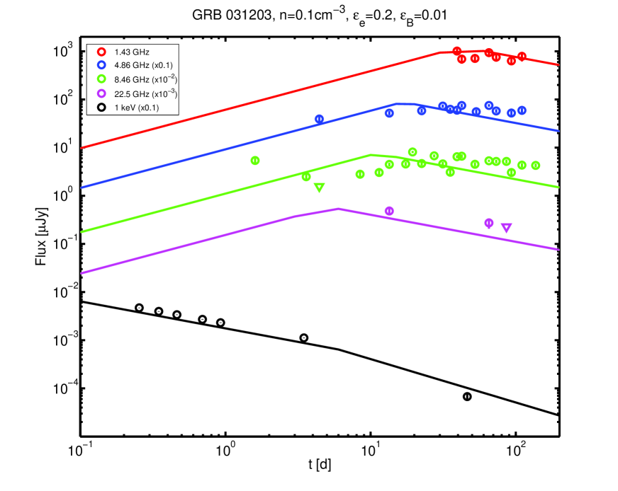
Figure 1: The observed and predicted radio and X-ray afterglows of GRB 031203. The fit shown is for $E_{f,0}=10^{50}$ erg, $\gamma_{f,0}=5$, $s=2.1$, $p=2.4$, $\epsilon_{e}=0.2$, $\epsilon_{B}=0.01$ and an ISM density with $n=0.1$cm^-3. Here and in the rest of the figures, circles denote observations, vertical lines within the circles denote flux errors and triangles are upper limits.

GRB 031203 was monitored extensively in the radio bands (Soderberg et al., 2004), and it was also followed in the X-ray band starting 6 hours after the burst (Watson et al., 2004). We calculate the predicted radio fluxes in the ISM scenario and present them in Fig. 1. We find that the model can fit both the radio and also the X-ray observations quite well.

We find that the X-ray band before 6 days is above $\nu_{m}$ but below $\nu_{c}$. It decreases as $\propto t^{-0.55\pm 0.05}$ (Watson et al., 2004). The closure relations in eq. (20) yield a consistent temporal decay with the chosen value of $p=2.4$. Within this model, the reason why the X-ray light curve steepens at $\sim 6$ days is due to the crossing of the synchrotron cooling frequency through the X-ray observing band (the synchrotron cooling frequency decreases with time in this case). The observed X-ray spectrum at $t<6$ days is $\beta_{x}=0.9\pm 0.05$ and $0.7\pm 0.2$ at 6 hours and 3 days, respectively (Watson et al., 2004), roughly consistent with the predicted spectrum $\beta_{x}=(p-1)/2=0.7$. The X-ray spectrum after $\sim 6$ days should steepen by $\Delta\beta_{x}=0.5$, which can be tested with the Chandra data at $\sim 50$ days (Fox et al., 2004).

The blast wave energy, which changes with time as energy is injected, is $\sim 2\times 10^{50}$ erg at 10 days in this case; the time dependence of the blast wave energy can be found in eq. (10). The non-relativistic phase for this burst will commence beyond 300 days, which is a factor of few larger than the time of the last observations and all the light curves would slightly rise. We note that solutions with a slightly smaller density and larger $\epsilon_{B}$ also fit the data well and the non-relativistic phase might be delayed for an even longer time.

The wind case is not able to fit the radio observations, even if we allow $\epsilon_{e}$ to vary from the fiducial adopted value of $\epsilon_{e}=0.2$. Also, the radio light curves would be steeper than $\propto t^{-1.1}$ for $2<p<3$, according to eq. (20), which is much steeper than observed (the radio light curves are quite flat at late times). We therefore do not show a figure for this scenario.

Interestingly, IR-optical observations starting 9 hr after the burst show a bright IR emission with a very steep soft spectrum, $F_{\nu}\propto\nu^{-2.36}$ (Malesani et al., 2004). This emission fades within a day, before the main component of the supernova (SN) light rises a week later. The very soft spectrum of early IR emission indicates that it has, most likely, a different origin than that of both the radio and the X-rays. It is still consistent with the radio and X-ray being both generated by synchrotron emission, as our model predicts an IR flux that is fainter by a factor of $\sim 10$ than the one observed. We do not discuss here the origin of this unique IR emission, as it is most likely related to the cooling envelope phase of the SN. In that case the bright yet fast fading signal may indicate on a progenitor composed of a compact core and an extended low-mass envelope (Nakar & Piro, 2014).

Soderberg et al. (2004) have modeled the radio emission of this burst in the context of the external forward shock emission (without energy injection). They also prefer an ISM with similar density as the one we adopt here. However, energy injection via the blast wave enables us explain also the X-ray emission, which Soderberg et al. (2004) had found was a factor of $\lower 2.0pt\hbox{$\,\buildrel\scriptstyle<\over{\scriptstyle\sim}\,$}10$ smaller than observed.

4.3 GRB 980425

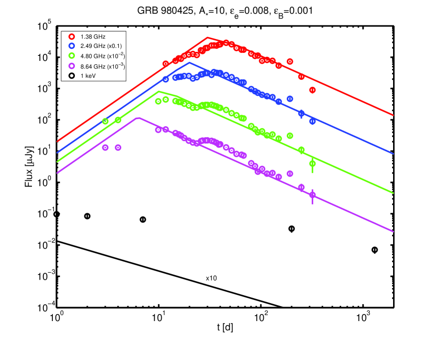
Figure 2: The observed and predicted radio and X-ray afterglows of GRB 980425. The fit shown uses $E_{f,0}=6\times 10^{48}$ erg, $\gamma_{f,0}=3$, $s=2.1$, $p=2.8$, $\epsilon_{e}=0.008$ and $\epsilon_{B}=0.001$. This model corresponds to the wind case with $A_{*}=10$, which can fit the overall trend of the radio observations (albeit with a small value of $\epsilon_{e}$), but the X-ray prediction lies below the observations (we have multiplied the X-ray expectations of the model by a factor of 10). Using the same parameters, but allowing for a smaller value of $p$ to model the X-rays ($p=2.1$) yields an X-ray flux consistent with observations.

GRB 980425 was monitored extensively in the radio bands (Kulkarni et al., 1998), and its X-ray data showed an unusually flat behavior for more than 100 days (Pian et al., 2000; Kouveliotou et al., 2004). We use the scenario described above for the parameters of this llGRB to model the radio light curves. The initial blast wave energy of this llGRB is the smallest of all llGRBs, therefore, we need to consider the non-relativistic phase since $t_{NR}$ falls within the available radio observations for $n\lower 2.0pt\hbox{$\,\buildrel\scriptstyle>\over{\scriptstyle\sim}\,$}0.01$ cm^-3 ($A_{*}\lower 2.0pt\hbox{$\,\buildrel\scriptstyle>\over{\scriptstyle\sim}\,$}0.01$) in the ISM (wind) case, see eq. (11).

We consider first the ISM case. The light curves above the minimum frequency in the non-relativistic phase increase with time, see eq. (23), which is inconsistent with the time-decreasing trend of the radio data at late times. Therefore, we consider the wind medium, for which the solution lies entirely in the non-relativistic phase. Using a value of $\epsilon_{e}=0.2$ as discussed above, we find that the wind medium is not able to fit the radio observations. We lower $\epsilon_{e}$ to a smaller value ($\epsilon_{e}\sim 0.01$) and find that the predicted light curves give an overall good fit to the radio observations (however, the radio observations at $<10$ days and the slight increase in flux at $\sim 30$ days are not well fit). We note that the radio light curves beyond $\sim 30$ days are above $\nu_{a}$ and $\nu_{m}$, but still below $\nu_{c}$. Observations indicate that they decrease roughly as $\propto t^{-1.6}$ (Li & Chevalier, 1999). Using the closure relations in eq. (23), we find that a value of $p\approx 2.8$ fits the decay of the radio observations, and we present the light curves in Fig. 2 for this case. The predicted X-ray emission (which lies above $\nu_{c}$) is smaller than the observed value by at least a factor of a few tens. The blast wave energy at 10 days in this case is $\sim 3\times 10^{50}$ erg; the time dependence of the blast wave energy can be found in eq. (16).

Interestingly, in the wind case and using the same parameters as above, but changing the value of $p$ to $p\approx 2.1$, we find an X-ray flux consistent with the observations, both in normalization and temporal decay. The X-ray light curve until $\sim 200$ days decays as $\propto t^{-0.16\pm 0.04}$ (Pian et al., 2000), but including the flux at $\sim 1000$ days, the overall light curve decays as $\sim t^{-0.33}$. This is consistent with the predicted temporal decay $\propto t^{-0.4}$, according to eq. (23). The observed X-ray spectrum for $t\lower 2.0pt\hbox{$\,\buildrel\scriptstyle<\over{\scriptstyle\sim}\,$}200$ days is $\beta=1.0\pm 0.3$ (Pian et al., 2000), consistent with the predicted value of $\beta=p/2\approx 1.1$. The predicted radio light curve with $p=2.1$ would be too shallow ($\propto t^{-0.9}$), but would qualitatively fit the radio observations within a factor of $\lower 2.0pt\hbox{$\,\buildrel\scriptstyle<\over{\scriptstyle\sim}\,$}2$ until $\sim 100$ days, and the discrepancy would increase up to a factor of $\lower 2.0pt\hbox{$\,\buildrel\scriptstyle<\over{\scriptstyle\sim}\,$}10$ at $\sim 300$ days. These results suggest that both the radio and the X-rays can be generated by synchrotron emission from a single population of electrons in the forward shock, if the electron spectrum is concave. Namely, if the electron spectrum is steep (soft) at low energies and shallow (hard) at high energies. Such spectrum is predicted by some Fermi acceleration models in Newtonian shocks, due to the nonlinear feedback of the accelerated particles on the shock structure (e.g., Bell, 1987).

Li & Chevalier (1999) have modeled the radio data of GRB 980425 also in the wind case and they present several solutions: One with $\epsilon_{e}=\epsilon_{B}=0.1$ and $A_{*}\approx 0.04$, another with $\epsilon_{e}\sim 1$, $\epsilon_{B}=10^{-6}$ and $A_{*}\approx 6$, and they also find acceptable models with $\epsilon_{e}\sim 0.01$. Our solution for this GRB has $\epsilon_{e}=0.01$, however, the two models are inherently different. Li & Chevalier (1999) allow for the energy of the blast wave to increase instantaneously by a factor of $\sim 2.5$ to explain the increase by a factor of $\sim 2$ in the radio light curves at $\sim 30$ days. However, within out model energy is continuously injected to the blast wave and we ignore this slight increase in the radio light curves at $\sim 30$ days.

4.4 GRB 060218

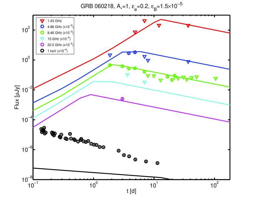
Figure 3: The observed and predicted radio and X-ray afterglows of GRB 060218. The fit shown uses $E_{f,0}=2\times 10^{50}$ erg, $\gamma_{f,0}=1.3$, $p=2.6$, $\epsilon_{e}=0.2$ and $\epsilon_{B}=1.5\times 10^{-5}$. This model corresponds to the synchrotron emission from the breakout shell during the coasting phase for a wind with $A_{*}=1$, which can qualitatively fit the radio observations. However, the model underpredicts the X-ray emission (and, even if the X-ray would not be underpredicted, the model cannot explain the steep observed X-ray spectrum).

The Lorentz factor of the breakout shell for this burst is close to unity and creation of pairs in the shock is marginal. Therefore, it is likely that no shells are accelerated to velocities faster than the breakout shell, in which case the forward shock is coasting at a constant velocity for a long time until the breakout shell decelerates. In this case only a wind medium can fit the observed decaying radio afterglow and this is the model we consider here. The blast wave moves with a constant Lorentz factor of $\sim 1.3$ until it decelerates at $\sim 200$ days. During the coasting phase the blast wave energy increases linearly with time for the wind case, and reaches $2\times 10^{50}$ erg at the deceleration time. We note that solutions with a smaller density also fit the data well (and also underestimate the X-ray fluxes) and the deceleration phase might be delayed for an even longer time.

Radio and X-ray afterglow observations of GRB 060218 have been reported in Campana et al. (2006); Soderberg et al. (2006); Evans et al. (2007, 2009). The radio light curve at 8.46 GHz decays as $\propto t^{-0.8}$ (Soderberg et al., 2006). We find that this radio band is between $\nu_{a}$ and $\nu_{c}$ ($\nu_{m}$ is below $\nu_{a}$). Using eq. (17), we find that a value of $p\approx 2.6$ fits the decay of the radio observations, and this is the reason we present the light curves for this value of $p$ in Fig. 3. We find an overall good fit to the radio observations (however, some upper limits at 1.43, 4.86 and 8.46 GHz are consistent only to within a factor of $\lower 2.0pt\hbox{$\,\buildrel\scriptstyle<\over{\scriptstyle\sim}\,$}2$). We also find $\nu_{a}\sim 4$ GHz at 5 days, and that $\nu_{m}$ is about ten times smaller than $\nu_{a}$, consistent with the spectrum at 5 days presented in Soderberg et al. (2006). With that model the predicted X-ray emission is below the observed value by at least a factor of $\sim 10$.

As in the case of GRB 980425, we lower the value of $p$ to obtain a rough estimate if a concave electron spectrum may fit the radio and X-ray data simultaneously. This increases the predicted X-ray flux, although, it makes the light curve shallower, see eq. (17), which is inconsistent with the observed decay $\propto t^{-1.2\pm 0.1}$ (Campana et al., 2006). Nevertheless, the discrepancy between the predicted and observed X-ray flux shrinks with a smaller value of $p$.

Even if such a modification would be capable of explaining the X-ray flux, the predicted X-ray spectrum is $\beta_{x}=(p-1)/2\approx 0.8$. This stands in contrast with the observed X-ray spectrum $\beta_{x}\approx 2.2\pm 0.2$ (Soderberg et al., 2006). Such a steep spectrum cannot be explained within this model, unless the electron spectrum has a cut-off at energies of the X-ray emitting electrons. This solution is contrived, and we conclude that the X-ray and the radio are most likely of different origin.

If faster shells than the breakout shell are present, then the blast wave would start decelerating at much earlier times and it can be relativistic for long enough for the decreasing radio emission to be consistent also with a constant density medium. However, in that case $\nu_{a}<1.43$ GHz $<\nu_{m}$ at 5 days, which leads to a flux at 1.43 GHz that is at least a factor of $\sim 3$ brighter than the upper limit at that time. This is marginal even if there is strong scintillation, but cannot be completely ruled out. The X-ray emission in that case is still underpredicted by the model if a single electron power-law is assumed and the difficulty to reproduce the X-ray spectrum persists.

4.5 GRB 100316D

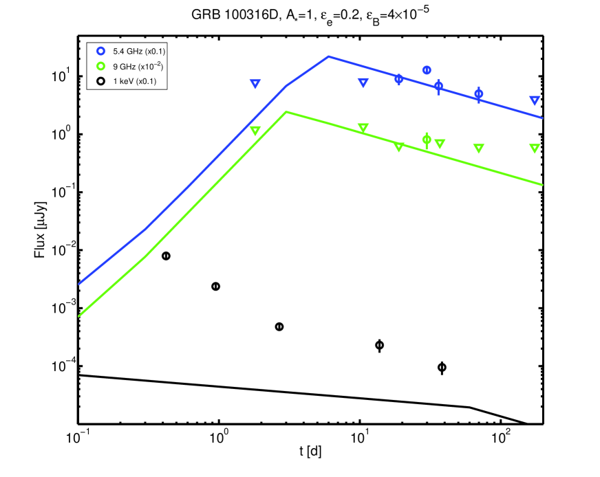
Figure 4: The observed and predicted radio and X-ray afterglows of GRB 100316D. The fit shown uses $E_{f,0}=2\times 10^{50}$ erg, $\gamma_{f,0}=1.3$, $p=2.4$, $\epsilon_{e}=0.2$ and $\epsilon_{B}=4\times 10^{-5}$. This model corresponds to the synchrotron emission from the breakout shell during the coasting phase for a wind with $A_{*}=1$, which can qualitatively fit the radio observations (we note that the radio data are sparse and only available in two frequencies, so drawing strong conclusions is difficult). However, the model underpredicts the X-ray emission (and, even if the X-ray would not be underpredicted, the model cannot explain the steep observed X-ray spectrum).

The last burst in our sample is GRB 100316D, whose X-ray data are presented in Evans et al. (2007, 2009); Starling et al. (2011), and additional X-ray data and the radio data are presented in Margutti et al. (2013). Since this burst is almost identical to GRB 060218, and it is explained with the same parameters within the relativistic shock breakout model, we use the same afterglow model, namely synchrotron emission from a coasting blast wave in a wind medium. The radio data of this burst are sparse, available only in two frequencies and possibly affected by scintillation. Therefore, it is not very constraining and many models can fit the radio data. Here we present one such model in Fig. 4, which fits the radio data reasonably well. Most importantly, $\nu_{a}$ is not well constrained, e.g., Margutti et al. (2013) suggest that $\nu_{a}\sim 5$ GHz at $\sim 30$ days, whereas in the model presented here this value of $\nu_{a}$ is obtained at $\sim 6$ days. As a result the radius and thus the velocity of the radio emitting region can significantly vary between various acceptable models.

The model underpredicts X-ray flux compared with the observed value by a factor of more than $\sim 4$. As for GRB 060218, a smaller value of $p$ (concave electron spectrum) increases the predicted X-ray flux, but the X-ray light curve is too shallow and it is inconsistent with the observed decay $\propto t^{-0.87\pm 0.08}$ (Margutti et al., 2013). At the same time the observed X-ray spectrum, $\beta_{x}\approx 2.49\pm 0.26$ (Margutti et al., 2013), is similar to that of GRB 060218 and it indicates that also here the X-ray and the radio are most likely generated by different processes.

The blast wave moves with a constant velocity and its energy increases linearly with time until it reaches $2\times 10^{50}$ erg at the deceleration time of $\sim 200$ d. We note that solutions with a smaller density also fit the data well (and also underestimate the X-ray fluxes) and the deceleration phase might be delayed for an even longer time. If faster shells than the breakout shell would be present, then an ISM or wind medium would also marginally fit the radio data, since the data are not very constraining.

Soderberg et al. (2006); Fan, Piran & Xu (2006) have modeled the radio emission of GRB 060218, and Margutti et al. (2013) the one of GRB 100316D in the context of the external forward shock emission. The external densities they find are different than ours. However, here the afterglow is produced in the coasting phase, whereas they considered a decelerating blast wave.

5 Constraints on the X-ray source

The X-ray afterglows in GRB 060218 and GRB 100316D are most likely not generated by the same process that produces their radio emission. Nevertheless, several strong constraints on the X-ray source can be derived from simple considerations. These constraints are regardless of whether llGRBs are shock breakouts or not, or even of the exact models of both the radio and the X-ray emission.

In both bursts the total energy emitted in X-rays by $10^{6}$ s is $\sim 10^{48}$ erg (assuming isotropy; see below). Thus, the first general constraint is that for any reasonable radiative efficiency, the source energy at that time is $>10^{49}$ erg, and most likely significantly higher. The X-ray energy output is roughly constant for every logarithmic time interval, implying that the energy constraint at $10^{4}$ s is lower by about an order of magnitude.

A second constraint follows from the fact that the gamma-ray emission, which led to the bursts’ detection, is not highly collimated, namely opening angle $>30^{\circ}$ and inverse beaming factor $<10$ (e.g., Soderberg et al., 2006). Given that the X-ray emission is seen in both bursts, it is most likely not highly collimated as well. This implies that the source cannot be a highly relativistic narrow jet. In fact, the radio emission implies that the X-ray source cannot be highly relativistic even if it is not narrowly collimated. The reason is that without being collimated it cannot run ahead of the radio source, otherwise it will sweep the circum-burst medium, thereby preventing the interaction that leads to the radio emission. Now, the radio source, at least in GRB 060218 where $\nu_{a}$ is measured, is mildly relativistic. Therefore, the X-ray source is at most mildly relativistic, implying that the X-ray emission radius, $R_{x}$, is limited to $R_{x}\lower 2.0pt\hbox{$\,\buildrel\scriptstyle<\over{\scriptstyle\sim}\,$}ct$.

On the other, hand the X-ray emitting radius cannot be too low. The line profiles of SN 2006aj (the SN that accompanied GRB 060218) do not show signs of anisotropy, and there is no polarization ($<2$ per cent at the 3-$\sigma$ level) either in the lines nor in the continuum, implying that the bulk of the SN ejecta has no strong deviation from spherical symmetry (Mazzali et al., 2007). This ejecta is about a solar mass moving at a velocity $\lower 2.0pt\hbox{$\,\buildrel\scriptstyle>\over{\scriptstyle\sim}\,$}0.05$c (Pian et al., 2006; Bufano et al., 2012) that lies between the observer and the center of the explosion. No radiation that is emitted behind this mass can escape to the observer on a time-scale that is shorter than about a week (since the diffusion time is too long). Therefore, the X-ray source must be at all time ahead of the bulk of the SN mass. Thus, together with the limit that the radio emitting region is ahead of the X-ray source, we obtain $0.05ct\lower 2.0pt\hbox{$\,\buildrel\scriptstyle<\over{\scriptstyle\sim}\,$}R_{x}\lower 2.0pt\hbox{$\,\buildrel\scriptstyle<\over{\scriptstyle\sim}\,$}ct$. Given that the afterglow is observed over two decades in time, the radius of the region where X-rays are generated must increase in time together with the SN ejecta. This constraint implies that the X-ray source is most likely within the explosion ejecta, between the bulk of the SN mass (the slowest part of the ejecta) and the leading radio source (the fastest part of the ejecta). This disfavors emission models that are powered by internal dissipation in an unrelated component, such as internal shocks or magnetic reconnection in an outflow that is unrelated to the one producing the SN and the radio emission.

The constraints derived above are non-trivial and cannot be easily met by most types of X-ray sources. Specifically, they are most difficult to reconcile with any source that gains its energy continuously from a central engine, as has often been suggested (e.g. Soderberg et al., 2006; Fan, Piran & Xu, 2006; Margutti et al., 2013). The main problem in such sources is that the energy which is generated in the center must penetrate through several solar masses of SN ejecta, while the source is not relativistic and it is not narrowly collimated ($>30^{\circ}$). Furthermore, this should take place without the energy being dissipated below the photosphere and without leaving any major imprint on the asymmetry inferred from the SN line profiles.

We note that a simple “inward” extrapolation in energy (from the energy of the fast moving material to the SN energy) described at the end of Section 3.3 does not work. Namely, the energy-velocity relation is too shallow compared to that seen in regular SNe and to that expected in a simple spherical blast wave that propagates in a typical star (e.g., Soderberg et al., 2006; Margutti et al., 2013). This is true even when one accounts for the shallow relativistic slope described here and in previous works (e.g., Tan et al., 2001). This probably implies that the explosion is not fully spherical (e.g., Couch et al., 2011; Matzner et al., 2013; Salbi et al., 2014), or that the stellar structure is different than in typical SNe, or a combination of the two. A likely explanation for this point is discussed in a future work (Nakar, in preparation). Regardless of the reason for the shallow energy profile, the observations indicate that the asphericity, if exists, is not high (inverse beaming factor $<10$) and that the spherical approximation for the gamma-ray emission and the following blast wave is reasonable. Note that if the breakout deviates from spherical symmetry this may result in breakout velocities that are slower in some parts of the stellar surface (Matzner et al., 2013; Salbi et al., 2014). But, unless the breakout asphericity is high, the breakout from most of the stellar surface will not be strongly affected; neither the resulting gamma-rays nor the following blast wave.

6 Discussion and Conclusions

We have calculated the synchrotron emission from the forward shock that arises during the interaction between the stellar ejecta and the circum-burst medium following a relativistic shock breakout. The hydrodynamics of the shock breakout ejecta is described following Nakamura & Shigeyama (2006), where we assumed that the progenitor has a standard radiative stellar envelope, characterized by a polytropic index $n=3$. For the subsequent blast wave evolution we assume that the circum-burst density profile is either constant (ISM) or $\propto r^{-2}$ (wind). The main difference between this model and the standard GRB afterglow model is that here energy is continuously injected into the slowly decelerating blast wave by slower ejecta whose profile is dictated by the SN shock that unbinds the stellar envelope. Once the behavior of the blast wave is determined the emission follows the standard GRB synchrotron afterglow model (Sari et al., 1998).

We have applied this model to the four llGRBs with good data, GRBs 980425, 031203, 060218 and 100316D. The prompt emission provides us the initial conditions (the energy and Lorentz factor profiles) of the ejecta (Nakar & Sari, 2012). We first fit, for each burst, the free parameters of the emission model to the observed radio afterglow and then check if the same model parameters can also explain the observed X-ray afterglow. We find that the model can successfully explain the radio emission of all four llGRBs. In some llGRBs, the X-ray emission can also be generated by the same population of electrons that generate the radio emission, while in others it cannot.

For GRB 031203, we find that the simplest model can successfully fit both the observed radio and X-ray afterglows light curves and spectra with a single set of parameters, if the external medium is an ISM. This burst is the only llGRB for which we expect the blast wave producing the afterglow to be relativistic, similarly to regular GRBs, and indeed the parameters we find for the external density and microphysical parameters are similar to those found in regular GRBs. This is the first time that both the prompt and the afterglow emission can be explained for a single llGRB: The prompt emission is produced by the relativistic shock breakout signal and the radio and X-ray afterglow are explained by its accompanying external shock.

For GRB 980425, a model with a wind medium fits the radio data. The density of the wind is such that the blast wave is already Newtonian at the time of the first observation. Using the simplest model, the same parameters that fit the radio data result in an X-ray spectrum that is too soft and an X-ray flux that is too low. However, the model can simultaneously explain the radio and X-ray observations (both the light curve and the spectrum) with a minor modification that relaxes the assumption of a single power-law electron distribution. A concave electron distribution with a logarithmic derivative of $p\approx 2.8$ for the radio emitting electrons and $p\approx 2.1$ for the X-ray emitting electrons can fit both observations. Interestingly such a spectrum is predicted by some Fermi acceleration models in Newtonian shocks, due to nonlinear feedback of the accelerated particles on the shock structure (e.g., Bell, 1987).

For GRB 060218 and 100316D, the relativistic shock breakout model predicts a mildly relativistic breakout that is consistent with the absence of ejecta faster than the breakout shell. In that case the breakout shell decelerates after a long time, and the observed afterglow is produced via synchrotron emission in the coasting phase. The observed radio afterglow, which decays at late times, is consistent only with a wind medium (in the ISM case all light curves rise during the coasting phase). This model is able to fit the radio data. However, with the same parameters, it underestimates the X-ray flux. Moreover, the afterglow X-ray spectra in these two bursts are very steep. In fact, it is very peculiar compared to other GRB afterglows. Yet, the light curve in both cases (a very bright simple power-law, roughly $\propto t^{-1}$) resembles that of regular GRBs and is uncommon in ordinary SNe. The steep spectra implies, first, that it is highly unlikely that the X-rays and the radio are generated by the same population of electrons, as was already found earlier (Fan, Piran & Xu, 2006; Soderberg et al., 2006; Margutti et al., 2013). Secondly, the combination of the X-ray spectra and light curves in these two bursts, suggests that the X-ray source is uncommon to either regular GRBs or regular SNe.

We stress that while we have found models that are consistent with the radio emission of all four llGRBs, these are by no means the only consistent models. First, within the synchrotron forward shock model there is enough freedom to allow for a range of parameters that fit the observations. Secondly, we did not attempt to calculate here the synchrotron emission from the reverse shock or the contribution of inverse Compton emission from either the forward or the reverse shocks. It is most likely that there are solutions where the observed radio emission is dominated by one of these components (e.g., reverse shock synchrotron).

The main puzzle that remains is the source of the X-ray afterglow in llGRBs 060218 and 100316D. We draw here some general constraints on the source of this emission, finding that it is not narrowly collimated and that it is not ultra-relativistic. The source itself is most likely moving at velocity $>0.05$c and a Lorentz factor $<2$, and it is located at all time somewhere within the ejecta, between the bulk of the SN mass and the leading radio source. Previous authors invoked the existence of a continuous central engine to explain the X-ray afterglow (Soderberg et al., 2006; Fan, Piran & Xu, 2006; Margutti et al., 2013), without discussing how such a source produces this emission. The constraints we derive here show that long lasting central engine activity is unlikely to be the correct solution. The major difficulty for this model is the need for the central engine energy, that is not narrowly collimated, to penetrate through the opaque SN ejecta without leaving a trace of anisotropy in the spectral line profiles (Mazzali et al., 2007). Additionally, the combination of the X-ray light curve and spectrum seen in these bursts is unique and does not resemble any other cases where we have a good reason to suspect that they are a result of central engine activity. In our view, given that the X-ray source is probably moving together with the ejecta, the most natural scenario is that the X-ray source is within the interaction layer that is also responsible for the radio emission. Since the X-ray and the radio do not arise from the same process, it is possible that either the long lived reverse shock (within a refreshed shocks scenario) or inverse Compton emission can explain these unique X-ray signatures.

References

- Barniol Duran, Nakar & Piran (2013) Barniol Duran, R., Nakar, E., Piran, T., 2013, ApJ, 772, 78
- Bell (1987) Bell, A.R., 1987, MNRAS, 225, 615
- Bromberg et al. (2011) Bromberg, O., Nakar, E., Piran, T., 2011, ApJ, 739, L55
- Bufano et al. (2012) Bufano, F. et al. 2012, ApJ, 753, 67
- Campana et al. (2006) Campana, S. et al., 2006, Nature, 442, 1008
- Chevalier (1982) Chevalier, R.A., 1982, ApJ, 258, 790
- Cobb et al. (2006) Cobb, B.E., Bailyn, C.D., van Dokkum, P.G., Natarajan, P., 2006, ApJ, 645, L113
- Cohen & Piran (1999) Cohen, E., Piran, T., 1999, ApJ, 518, 346
- Colgate (1974) Colgate, S.A., 1974, ApJ, 187, 333
- Couch et al. (2011) Couch, S.M., Pooley, D., Wheeler, J.C., Milosavljevic, M., 2011, ApJ, 727, 104
- Coward (2005) Coward, D.M., 2005, MNRAS, 360, L77
- Ensman & Burrows (1992) Ensman, L., Burrrows, A., 1992, ApJ, 393, 742
- Evans et al. (2007) Evans, P.A. et al., 2007, A&A, 469, 379
- Evans et al. (2009) Evans, P.A. et al., 2009, MNRAS, 397, 1177
- Falk (1978) Falk, S.W., 1978, ApJ, 225, L133
- Fan, Piran & Xu (2006) Fan, Y.-Z., Piran, T., Xu, D., 2006, JCAP, 9, 13
- Fan et al. (2011) Fan, Y.-Z., Zhang, B.-B., Xu, D., Liang, E.-W., Zhang, B., 2011, ApJ, 726, 32
- Fox et al. (2004) Fox, D.B., Soderberg, A.M., Kulkarni, S.R., Frail, D., 2004, GCN Circ. 2522
- Galama et al. (1998) Galama, T.J. et al, 1998, Nature, 395, 670
- Granot & Sari (2002) Granot, J., Sari, R., 2002, ApJ, 568, 820
- Guetta & Della Valle (2007) Guetta, D., Della Valle, M., 2007, ApJ, 657, L73
- Imshennik et al. (1981) Imshennik, V.S., Nadezhin, D.K., Utrobin, V.P., 1981, Ap&SS, 78, 105
- Johnson & McKee (1971) Johnson, M.H., McKee, C.F., 1971, Phys. Rev. D, 3, 858
- Kaneko et al. (2007) Kaneko, Y. et al., 2007, ApJ, 654, 385
- Katz et al. (2010) Katz, B., Budnik, R., Waxman, E., 2010, ApJ, 716, 781
- Katz et al. (2012) Katz, B., Sapir, N., Waxman, E., 2012, ApJ, 747, 147
- Klein & Chevalier (1978) Klein, R.L., Chevalier, R.A., 1978, ApJ, 223, L109
- Kouveliotou et al. (2004) Kouveliotou C. et al., 2004, ApJ, 608, 872
- Kulkarni et al. (1998) Kulkarni, S.R. et al., 1998, Nature, 395, 663
- Kumar & Piran (2000) Kumar, P., Piran T., 2000, ApJ, 532, 286
- Kyutoku et al. (2014) Kyutoku, K., Ioka, K., Shibata, M., 2014, MNRAS, 437, L6
- Leventis et al. (2012) Leventis, K., van Eerten, H.J., Meliani, Z., Wijers, R.A.M.J., 2012, MNRAS, 427, 1329
- Li & Chevalier (1999) Li, Z.-Y., Chevalier, R.A., 1999, ApJ, 526, 716
- Liang et al. (2007) Liang, E., Zhang, B., Virgili, F., Dai, Z.G. 2007, ApJ, 662, 1111
- Malesani et al. (2004) Malesani, D. et al., 2004, ApJ, 609, L5
- Margutti et al. (2013) Margutti, R. et al., 2013, ApJ, 778, 18
- Matzner & McKee (1999) Matzner, C.D., McKee, C.F., 1999, ApJ, 510, 379
- Matzner et al. (2013) Matzner, C.D., Levin, Y., Ro, S., 2013, ApJ, 779, 60
- Mazzali et al. (2006) Mazzali, P.A. et al., 2006, Nature, 442, 1018
- Mazzali et al. (2007) Mazzali, P.A. et al., 2007, ApJ, 661, 892
- Nakayama & Shigeyama (2005) Nakayama, K., Shigeyama, T., 2005, ApJ, 627, 310
- Nakamura & Shigeyama (2006) Nakamura, K., Shigeyama, T., 2006, ApJ, 645, 431
- Nakar & Piran (2011) Nakar, E., Piran, T., 2011, Nature, 478, 82
- Nakar & Sari (2010) Nakar, E., Sari, R., 2010, ApJ, 725, 904
- Nakar & Sari (2012) Nakar, E., Sari, R., 2012, ApJ, 747, 88
- Nakar & Piro (2014) Nakar, E., Piro, A.L., 2014, ApJ, 788, 193
- Pan & Sari (2006) Pan, M., Sari, R., 2006, ApJ, 643, 416
- Panaitescu et al. (1998) Panaitescu, A., Meszaros, P., & Rees, M.J., 1998, ApJ, 503, 314
- Panaitescu & Kumar (2000) Panaitescu, A., Kumar, P., 2000, ApJ, 543, 66
- Pian et al. (2000) Pian, E. et al., 2000, ApJ, 536, 778
- Pian et al. (2006) Pian, E. et al., 2006, Nature, 442, 1011
- Rees & Meszaros (1998) Rees, M.J., Meszaros, P., 1998, ApJ, 496, L1
- Sakurai (1960) Sakurai, A., 1960, Commun. Pure Appl. Math., 13, 353
- Salbi et al. (2014) Salbi, P., Matzner, C.D., Ro, S., Levin, Y., 2014, ApJ, 790, 71
- Santana et al. (2014) Santana, R., Barniol Duran, R., Kumar, P., 2014, ApJ, 785, 29
- Sari (1997) Sari, R., 1997, ApJ, 489, L37
- Sari et al. (1998) Sari, R., Piran, T., Narayan, R., 1998, ApJ, 497, L17
- Sari & Meszaros (2000) Sari, R., Meszaros, P., 2000, ApJ, 535, L33
- Sazonov et al. (2004) Sazonov, S.Yu., Lutovinov, A.A., Sunyaev, R.A., 2004, Nature, 430, 646
- Shen & Matzner (2012) Shen, R., Matzner, C.D., 2012, ApJ, 744, 36
- Soderberg et al. (2004) Soderberg, A.M. et al., 2004, Nature, 430, 648
- Soderberg et al. (2006) Soderberg, A.M. et al., 2006, Nature, 442, 1014
- Starling et al. (2011) Starling, R.L.C. et al., 2011, MNRAS, 411, 2792
- Tan et al. (2001) Tan, J.C., Matzner, C.D., & McKee, C.F., 2001, ApJ, 551, 946
- Virgili et al. (2009) Virgili, F.J., Liang, E.-W., Zhang, B., 2009, MNRAS, 392, 91
- Wanderman & Piran (2010) Wanderman, D., Piran, T., 2010, MNRAS, 406, 1944
- Wang et al. (2007) Wang, X.-Y., Li, Z., Waxman, E., Meszaros, P., 2007, ApJ, 664, 1026
- Watson et al. (2004) Watson, D. et al., 2004, ApJ, 605, L101
- Waxman et al. (2007) Waxman, E., Meszaros, P., Campana, S., 2007, ApJ, 667, 351
- Weaver (1976) Weaver, T.A., 1976, ApJS, 32, 233