Observations of Umbral Dots and their Physical Models

Abstract

The Hinode satellite opens a new era to the sunspots research, because of its high spatial resolution and temporal stability. Fine scale structures in sunspots, called umbral dots (UDs), have become one of the hottest topics in terms of the close observation of the magnetoconvection.

In this paper, a brief review of observed properties of UDs is given based on the recent literature. UDs born in the periphery of the umbra exhibit inward migration, and their speeds are positively correlated with the magnetic field inclination. Longer-lasting UDs are tend to be larger and brighter, while lifetimes of UDs show no relation with their background magnetic field strength. UDs tend to disappear or stop its proper motion by colliding with the locally strong field region. The spatial distribution of UD is not uniform over an umbra but is preferably located at boundaries of cellular patterns. From our 2-dimensional correlation analysis, we measured the characteristic width of the cell boundaries ($\approx$0.5) and the size of the cells ($\approx$6).

Then we performed a simplified analysis to get statistics how the UD distribution is random or clustered using the Hinode blue continuum images. We find a hint that the UDs become less dense and more clustered for later phase sunspots. These results may be related to the evolutional change of the subsurface structure of a sunspot.

Based on these observational results, we will discuss their physical models by means of numerical simulations of magnetoconvection.

1 Introduction

The observation and analysis of sunspots have been performed passionately from the age of Galileo. Although we have an accumulation of more than 400 year’s observational data, the sunspot remains to be one of the biggest unsolved problem in the solar physics: We still do not reach a consensus about the subsurface structure of a sunspot, i.e., whether the magnetic field is clustering or monolithic (Gokhale & Zwaan, 1972; Parker, 1979; Solanki, 2003). How their strong magnetic field are born and what determines its lifetime?(Cheung et al., 2010; Rempel, 2011) Understanding the sunspot is highly important for the astrophysics, because violent solar activities in the strong magnetic field of sunspot are driven by a common mechanism with many cosmic eruptive events (accretion jets, stellar flares, auroras, …).

We find a new path for solving these problems in the research of fine scale bright points called umbral dots (UDs, Figure 1, reviews are found in Borrero & Ichimoto (2011)). UDs are transient brightenings observed in sunspot umbrae and pores, with typical scales of 300 km diameter and 10 min lifetime (Sobotka et al., 1997, 1997; Kitai et al., 2007; Riethmüller et al., 2008; Louis et al., 2012). The magnetic properties around UDs are studied by many authors (Riethmüller et al., 2008; Sobotka & Jurčák, 2009; Watanabe et al., 2012), and they reach a consensus that UDs exhibit local reduction of field strength at deep layer. Upflow inside UDs and confined down-flowing regions outside of them are observed in recent high-resolution observations (Ortiz et al. 2010, Watanabe et al. 2012, Riethmüller et al. (2013)).

A UD is considered to be a natural consequence of the interaction between the convection and the magnetic field based on the monolithic sunspot model (Schüssler & Vögler, 2006; Bharti et al., 2010). One of the most sophisticated computer simulation of magnetoconvection performed by Rempel (2012) succeeded in reproducing the overall structure of the sunspot. The convective motions inside the umbra push out the boundary of the magnetic field lines inside the convective cell, creating a region of strongly reduced field strength, and forming a cusp or canopy field configuration. As UDs are strongly linked with the subsurface through an interaction with the deep convective layer, they have a potential to offer us information of the unreachable subsurface structure and its dynamics.

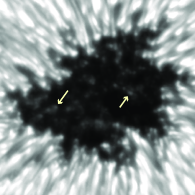
Figure 1: Blue continuum image of NOAA 10944 observed by the Hinode SOT on 2007 March 2. The FOV is about 17arcsec$\times$17arcsec. The arrows indicate two prominent UDs in the umbra.

The paper is organized as follows. The review of recent observational analyses, and our new analysis on the UD distribution are given in Section 2. In Section 3, we discuss how these observational results are consistently interpreted by means of numerical studies of magnetoconvection. Finally, based on the analysis and discussion, we conclude how the UD analysis can be one of the most important topics in the solar physics in Section 4.

2 Review of Recent Analyses

The observation of fine scale structure like UDs needs high spatial resolution. The Hinode Solar Optical Telescope (SOT) has a main mirror of 50-cm aperture and achieves its diffraction limit of 0.2-0.3 ALWAYS because of its seeing-free environment (Tsuneta et al., 2008; Suematsu et al., 2008). This temporal stability is the best advantage for reliable analysis on the structure’s temporal evolution. On the other hand, the Swedish Solar Telescope (SST, Scharmer et al. (2003)) has an effective aperture of 1-m, twice as large as that of the Hinode. Plus they possess a spectro-polarimetric imaging system called CRISP, which enables a scanning sequences of magnetic sensitive lines rapidly only in a few minutes intervals.

The analyses below utilizes the most optimum observations ever for their individual purposes.

2.1 Inward migration

UDs show an apparent motion of so-called inward migration toward the center of the umbra. An important question we have to answer is that why the UDs migrate always inward to the umbra center , and why they are better seen in the umbral periphery. Watanabe et al. (2009) analyzed the apparent motion speed of more than 2000 UDs and compared them to their background umbral field inclination. The field inclination is vertical at the center of the umbra, and becomes more inclined at the periphery. A positive correlation between the field inclination and speed of UDs are found (Figure 3). Least-square linear fitting for the samples with lifetime longer than 100 s gives us the following relations:
$V$ = 0.014 $\times$ $i$ (field inclination [degree]) + 0.070
and
$V$ = $-0.49$ $\times$ $B$ (field strength [kG]) + 1.5
where $V$ is the apparent motion speed in unit of km s^-1.

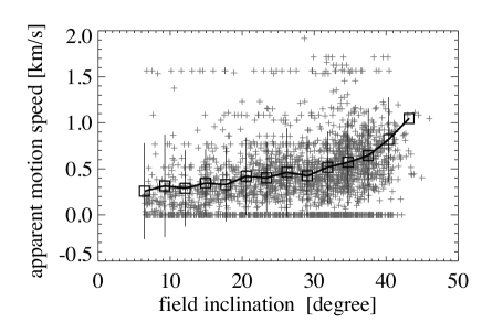
Figure 2: Scatter plots of field inclination versus the apparent motion speed of 2268 UD samples. The average bins of 3^∘ is shown with square symbols, and vertical solid line denote the standard error deviation errors. Modified from Figure 4 in Watanabe et al. (2009).

2.2 “Parameter survey” of magnetoconvective manifestation

As UDs are manifestation of magnetoconvection and they occur in various environmental magnetic field background, the observational characteristics of UDs can be used as “parameter survey” of magnetoconvection. Here we show some important plots showing how UD’s lifetime or radius depends on its environmental umbral field strength (Figure 3).

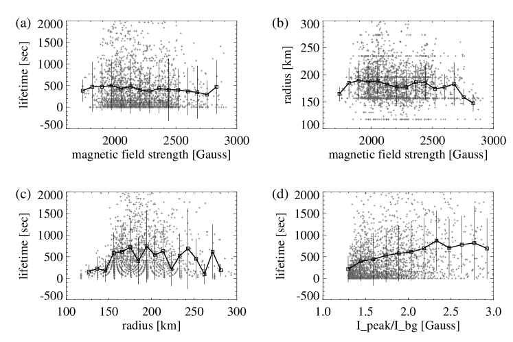
Figure 3: Scatter plots of (a) magnetic field strength versus lifetime (b) magnetic field strength versus radius (c) radius versus lifetime (d) peak intensity at UD normalized by the dark background intensity versus lifetime. There are 2268 UD samples. The averages for a proper binning size are shown with square symbols, and vertical solid line denote the standard error deviation errors. Extended from Figure 4 in Watanabe et al. (2009).

The lifetime of UDs scatter a lot and the average is almost constant regardless of the field strength and field inclination (not shown). The radius or the area of UDs, on the other hand, exhibits a weak hint of getting smaller in very strong ($>$2600 Gauss) fields. This is readily understood by the inhibition of expansion of buoyant plasma in the presence of the strong magnetic field pressure (Tian & Petrovay, 2013).

2.3 Evolution tracking

A detailed statistical work on the temporal evolution of UDs was performed by Watanabe et al. (2012). From the spectropolarimetric observation taken at SST/CRISP, maps of line-of-sight velocity and vector magnetic field around UDs are obtained. One example for a UD appeared in the central region of the umbra is shown in Figure 4. By seeing many UD movies, we found the following characteristics:

• The peak of continuum intensity and line-of-sight velocity coincides in time.

• The locations of UD appearance exhibit weakening of field strength compared with their surroundings in the growing phase of the UD. On the other hand, in the diminishing phase, UDs tend to collide into the pre-existing locally strong field regions.

• For the evolution of migrating UDs (e.g., Figure 17 in Watanabe et al. (2012)), they are preferentially located at the boundary of weak and strong field regions, and the boundary evolves with UD’s migration as if the leading edge of the UD is always blocked by strong field “walls”.

Sobotka et al. (1995) reported that the proper motion of peripheral or grain-origin UDs are influenced by the dark umbral cores: UDs slowed down and disappeared at the borders of dark umbral cores. Our third result is consistent with their result if we consider the dark umbral cores as the locally strong field regions.

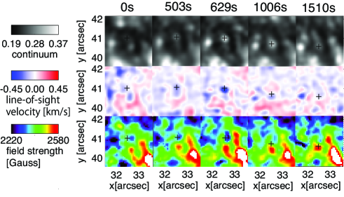
Figure 4: The temporal evolution of one central UD in continuum (top), line-of-sight velocity (middle), and magnetic field strength (bottom). The FOV is about 3$\times$3.5. The elapsed time from the emergence is shown at the top of the images. The black plus symbol indicate the UD position detected by the peak of the continuum. This UD disappears 1573 s after its emergence. Modified from Figure 13 in Watanabe et al. (2012).

2.4 Analysis on the theoretical UDs

A sophisticated work combining the observational data analysis with the simulated UDs was performed by Bharti et al. (2010). They first performed a 3-dimensional MHD simulation in a box filled by a fixed vertical field flux which corresponds to a mean field strength of 2500 G. Afterwards they applied a typical data analysis method on the simulated UDs. In this way, a direct compari?son with simulation and observation becomes possible.

The bottom panels (c) and (d) of Figure 3 are comparable to Fig.10 in Bharti et al. (2010). The radius or the area of smaller UD ($<$180 km) has a positive correlation between lifetime (c.f., the mean radius of our 2268 UDs is 183 km.), showing consistency with Bharti et al. (2010). However above 180 km radius, the correlation is missing. The lifetime become longer for brighter UDs, as is also consistent with Bharti’s results. Similar trends of size-lifetime and brighteness-lifetime relations are suggested by Sobotka & Puschmann (2009), while Riethmüller et al. (2008) do not find any systematical trend.

We can not compare Bharti’s result with the correlations in panels (a) and (b) in Figure 3, because the simulation pose a fixed vertical flux. However by M. Schüssler & A. Vögler (2006, private communication), the lifetime decreases as field strength gets larger if the amount of the fixed vertical flux is altered, which contradicts with the observation. On the other hand, the Stanford university group performed a numerical MHD simulations on solar magnetoconvection and found the opposite lifetime dependency, i.e., lifetime increases as field strength gets larger (Irina. N. Kitiashvili, private communication). Both the observation and simulation need more verifications to conclude this discussion.

2.5 Subsurface diagnosis

2.5.1 Cellar pattern

Watanabe et al. (2009) showed the map of the emergence positions of more than 2000 UDs (Figure 5). From Figure 5, we can recognize some cellular patterns in their distribution overlaid by thick dashed lines. These cellular patterns remind us of the cluster-type magnetic configuration (Parker, 1979), which the fields are separated into several bundles. Possibly they are the remnant of pores getting together in the developing phase of this sunspot. Tritschler & Schmidt (2002) and Sobotka et al. (1997) also concluded that the spatial distribution of UDs is not random but avoids dark umbral cores. On the other hand, Riethmüller et al. (2008) made a similar map of UD’s distribution and it showed a uniform distribution. At this point we do not reach to a consensus yet.

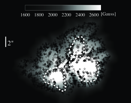
Figure 5: The emergence positions of 2268 UD samples overlaid on the background image of magnetic field strength. The thick dotted lines contours over some of the cellular patterns. Modified from Figure 6 in Watanabe et al. (2009). (color-version figure is available in the on-line material.)

We applied two-point correlation function method in order to quantify how the distribution is different from completely random one as a function of mutual distances between UDs. This method is also used for galaxies distribution observed by the Sloan Digital Sky Survey (Peebles, 1980). While the galaxies are in the 3-dimensional distribution, our UD distribution is in 2-dimensional plane. So the two-point correlation function can be reduced:

$$P(x_{1},x_{2})dx_{1}dx_{2}=\bar{n}[1+\xi(r)]dx_{1}dx_{2}$$ (1)

$P(x_{1},x_{2})dx_{1}dx_{2}$ is the probability that the both finite areas around the two point ($x_{1}$ and $x_{2}$, $r=|x_{2}-x_{1}|$) contains samples. $\bar{n}$ is the average number density of UDs, and $\xi(r)$ is called the two-point correlation function. If the distribution is completely random $\xi(r)$ is always zero. $\xi(r)$ can take negative values if the correlation is weaker. Or if we rewrite in the term of $r$ and the number of samples ($dN$) within the annular zone between $r$ and $r+dr$ around one sample, then

$$dN=2\pi r\bar{n}dr[1+\xi(r)]$$ (2)

It is important to accumulate $dN$ for as many samples as possible and calculate their average ${\overline{dN}}$ to get reliable statistics.

We applied this two-point correlation function calculation to the distribution of Figure 5, and the result is shown in Figure 6. We can get two hints from this plot. First, $\xi(r)$ is positive within distance smaller than 0.5. This is about 3 times longer than the typical radius of UDs, and may correspond to the element size of the clustering of UD occurrence. Or in other words, 0.5 corresponds to the width of of the cell boundaries or walls. Second, there is a broken branch of the log-log linear relation at around 6. It tells that there are a change in the pattern above the size of 6. Indeed the approximate diameter of the largest cellular pattern have the the diameter of $\approx$6. $\xi(r)$ rapidly decreases as it goes beyond 10, and this is because it gets close to the boundary of the sunspot periphery whose diameter is about 16.

Figure 6: Plots of two point correlation function ($\xi(r)+1$) versus distance ($r$) for the distribution of UDs in Figure 5 in log-log scale.

2.5.2 Statistical analysis of UD’s distribution

Here we perform another simplified analysis to describe the statistical characteristic of UD’s spatial distribution. We chose 16 sample sunspots arbitrary from 2013 June to August taken by the Hinode SOT blue continuum filtergrams. For each sample, we analyze only one snapshot image. All images have spatial pixel scale of 0.109 . The UD positions in each image are measured by eye within regions of continuum intensities darker than 0.4 $\times$ $I_{\textrm{qs}}$ (quiet-sun intensity) of background images (defined by smoothing the original image by 10 pixel $\times$ 10 pixel width). The area of the region, number of detected UDs, number density of UDs are listed in table LABEL:tbl:tbl2. Then we estimate the uniformity of the UD distribution. The concept is similar to the nearest neighbor method comparing to the Poisson distribution described in Clark & Evans (1954), but our uniformity ratio (U) is more appropriate for our spatially discrete samples

$$U=\frac{(\textrm{mean distance between nearest neighbors})}{2\sqrt{\frac{{\textrm{(area)}}}{\pi{\textrm{(number of sample)}}}}}$$ (3)

The concept of $U$ comes from the following context; Suppose the whole area is completely packed with small circles of the area divided by the number of sample. The diameter of this small circles is expressed as the denominator of the equation (3). If each sample is located at the center of these circles, this is the mostly scattered and uniform distribution, which is $U$=1. If $U$ is smaller than 1, the population is clustered. Typically the error of the detected number of UDs is about 5%, then the typical error of the ratio $U$ is about 2.5%.

Also in table LABEL:tbl:tbl2, we list up the phase of sunspot evolution classified roughly into four phases (0: just emerged, 1: evolving, 2: mature, 3: disintegrating) by tracking its temporal evolution using the helioviewer (http://www.helioviewer.org). Rough estimation of magnetic field strength is obtained by the daily sunspot drawings at the 150-Foot Solar Tower at Mt. Wilson Observatory (ftp://howard.astro.ucla.edu/pub/obs/drawings, Vaquero & Vázquez (2009)) in a unit one hundred gauss.

Table 1: Results of sunspot distribution analysis (during 2013 June-August)

time in UT	($x$,$y$)	sunspot	num. of	num. density	$U$	mag. field
	[arcsec]	phase∗A	UDs	[arcsec-2]	ratio	[$\times$100 G]∗B
Jun-14 10:38:06	(540, -210)	1	27	0.25	0.49	V23
Jun-14 10:38:06	(590,-200)	1	27	0.48	0.50	R23
Jun-15 09:23:20	(680,-220)	2	25	0.36	0.50	V20
Jun-15 09:23:20	(740,-210)	2	27	0.55	0.47	R21
Jul-05 02:51:27	(-530,-260)	2	64	0.19	0.45	R24
Jul-06 02:35:51	(-330,-260)	3	64	0.21	0.47	R24
Jul-25 02:43:03	(750,250)	2	12	0.30	0.54	V23
Jul-25 05:09:34	(270,-300)	1	16	0.63	0.55	R19
Jul-25 05:09:34	(290,-250)	1	38	0.63	0.58	V22
Jul-25 05:09:34	(330,-220)	1	11	0.59	0.56	R19
Jul-25 05:09:34	(380,-245)	1	29	0.65	0.64	R20
Jul-27 02:23:04	(640,-240)	2	55	0.82	0.53	V20
Aug-01 20:53:34	(80,-360)	0	12	0.56	0.45	R20
Aug-17 18:42:01	(470,-220)	2	119	0.50	0.52	R24
Aug-20 01:29:50	(820,-180)	3	34	0.31	0.42	R24
Aug-21 06:29:04	(-31,-250)	2	71	0.51	0.54	R24
*A: 0: just emerged, 1: evolving, 2: mature, 3: disintegrating, *B: V: negative polarity, R: positive polarity

Some scatter relations are shown in Figure 7. Although with large scatters, we found some hints that:

• Number density of UDs decreases as the magnetic field gets stronger.

• The distribution of UDs become more clustered (smaller $U$) for later phase sunspot than for earlier phase sunspot (except for one sample at phase = 0).

• Later phase sunspots have smaller number density.

• Distribution becomes more uniform (large $U$) for larger number density sunspot.

Figure 7: Scatter plots of (a) the magnetic field strength versus number density (b) the phase of sunspot evolution versus $U$ ratio (c) the phase of sunspot evolution versus number density (d) $U$ ratio versus number density. The dotted lines are linear fitting, and the number CC shows the correlation coefficient between the two variables. For the panel (b), both the fitting and CC are calculated excluding one data point at phase=0.

These statistical correlations suggest us a working view on the evolution of sunspot internal structures. When a sunspot is evolving, the umbral magnetic field is not uniform as the umbra is formed by aggregation of many pores with a variety of field strength. The spatial scale of inhomogeneity is small corresponding to the reminiscent of original components. At this phase, magnetic field is relatively weak, UDs are numerous, and distribute nearly uniformly. As the spot evolves, the small scale inhomogeneity of field strength gradually smoothed and strengthened, leading to the formation of large scale dark umbral cores where UDs are suppressed to appear. The degree of clustering will be large. Confirmation of this working view remains to the future more detailed analysis.

3 Model of UDs

The numerical simulation of UDs was successfully performed by Schüssler & Vögler (2006) in the framework of the magnetoconvection based on the monolithic sunspot model. Magnetoconvection can explain various manifestations in sunspots (UDs, light bridges, penumbral filaments) in a common way (Spruit & Scharmer, 2006; Scharmer & Spruit, 2006). Here we discuss the consistency between the model and the observational results.

We see many samples showing smooth transition from penumbral grains to UDs. The magnetoconvection model explains the different appearance of these structures by the change of convection cell shape in a large field inclination (Kitiashvili et al., 2009; Heinemann et al., 2007; Kitiashvili et al., 2011). In a large inclination situation, the convection cells become elongated while in a smaller inclination they are circular.

The inward migration is interpreted as the successive appearances of hot plasma plumes (Scharmer et al., 2008). When hot gas plume ascends from below, it bends the magnetic field line down (more inclined) at the surface locally, reducing the magnetic pressure there, and triggering a new appearance of hot gas. As the field is making in a fan-shape, their direction is always toward the center of the umbra. Accordingly it is readily understandable that there is positive correlation between the field inclination and the speed of inward migration, because this bending process does not occur in a vertical field situation.

The trend that longer-lasting UDs are brighter and larger is natural, if we suppose stronger and larger convective upflows for those UDs. However there is a discrepancy between observation and theory in the lifetime versus field strength relation (section 2.4). There are too large scatters in UD’s lifetime distribution in our observation. More precise definition of lifetime or larger statistics may give some relations as a future work.

The trend of disappearance/stopping at locally strong field region may correspond to the stronger suppression of convection there. However it is not easy to imagine the existence of strong field “wall” (boundary of weak and strong field) at the leading edge of migrating UD, which also migrate along with the motion of UD (section 2.3). Here we remind of the flux tube model (Schlichenmaier et al., 1998) which appeared for explaining penumbral Evershed flow by siphon flow mechanism. This model do not explain UDs, but it covers the mechanism of the penumbral grains. In the flux tube model, single flux tube located at the magnetopause is heated and get buoyant, and the footpoint of buoyant flux tube goes inward to the umbra. This migration of footpoint may correspond to the inward migration of the leading edge of penumbral grains. The strong field “wall” can be imagined as the compression of preexisting umbral field by the the buoyant flux tubes.

4 Conclusion

A UD is a unique cosmic phenomenon for understanding magnetoconvection with both spatially and temporarily resolved observations. Such studies that compare with the numerical simulation and the observed properties is possible owing to this rich data set (Bharti et al., 2010; Kilcik et al., 2012). There are other magnetoconvection manifestation in the universe, such as the accretion disk and the low temperature stars, although those are very far and so tracking the temporal evolution of their magnetoconvective cells is almost impossible. The observation of UD, in a sense, can be called as the “laboratory” of the magnetoconvection.

In this paper, we suppose the usability of a UD as a subsurface diagnosis. The most popular tool for a subsurface diagnosis is the helioseismology (Gizon et al., 2010; Moradi et al., 2010). However recently, Schunker et al. (2013) looked into the ability of helioseismology to probe the subsurface of sunspots, and they found that the subsurface magnetic field configuration below 2 Mm is not sensitive to the method of the helioseismology. We test the performance of two-point correlation function for the distribution of UD’s occurrence positions, and found a weak hint of cellular patterns with 6 diameter and 0.5 annular width. These patterns may corresponds to the flux bundles well below the sunspot as the cluster model predict. Although the well-known simulations of UDs (e.g., Schüssler & Vögler (2006)) are based on the monolithic sunspot model, we could not rule out the cluster sunspot model because UDs occur in shallow layers below umbra surface in their their simulations ($<$1 Mm), and their connection to deeper layer structure is still under investigation. We also introduce a simple parameter $U$ for describing the uniformity of the UD’s distribution. Our results tell that the distribution of UDs is more uniform in the earlier phase, and become more clustered in the later phase. It may represent that the global subsurface structure of a sunspot changes as time, because UDs occur in the interaction between the deep convective layer and magnetic field of a sunspot. The statistical analysis of UD’s distribution have a large potential to draw out information of the subsurface structure of a sunspot, and thus is worth to be extended further in the near future.

H. Watanabe wants to thank here Dr. Reizaburo Kitai, Dr. Kiyoshi Ichimoto, and Dr. Luis R. Bellot Rubio for their collaborative and supportive work. Our work was supported by the Grant-in-Aid for JSPS Fellows, and by the JSPS Core-to-Core Program 22001. Hinode is a Japanese mission developed and launched by ISAS/JAXA, with NAOJ as domestic partner and NASA and STFC (UK) as international partners. It is operated by these agencies in co-operation with ESA and NSC (Norway). This research has made extensive use of NASA’s Astrophysical Data System.

References

- Bharti et al. (2007) Bharti, L., Jain, R., & Jaaffrey, S. N. A. 2007, ApJ, 665, L79
- Bharti et al. (2010) Bharti, L., Beeck, B., & Schüssler, M. 2010, A&A, 510, A12
- Borrero & Ichimoto (2011) Borrero, J. M., & Ichimoto, K. 2011, Living Reviews in Solar Physics, 8, 4
- Cheung et al. (2010) Cheung, M. C. M., Rempel, M., Title, A. M., & Schüssler, M. 2010, ApJ, 720, 233
- Clark & Evans (1954) Clark, P. J., & Evans, F. C. 1954, Ecology, vol. 35, p. 445-453 (1954)., 35, 445
- Gizon et al. (2010) Gizon, L., Birch, A. C., & Spruit, H. C. 2010, ARA&A, 48, 289
- Gokhale & Zwaan (1972) Gokhale, M. H., & Zwaan, C. 1972, Sol. Phys., 26, 52
- Heinemann et al. (2007) Heinemann, T., Nordlund, Å., Scharmer, G. B., & Spruit, H. C. 2007, ApJ, 669, 1390
- Kilcik et al. (2012) Kilcik, A., Yurchyshyn, V. B., Rempel, M., et al. 2012, ApJ, 745, 163
- Kitai et al. (2007) Kitai, R., Watanabe, H., Nakamura, T., et al. 2007, PASJ, 59, 585
- Kitiashvili et al. (2009) Kitiashvili, I. N., Kosovichev, A. G., Wray, A. A., & Mansour, N. N. 2009, ApJ, 700, L178
- Kitiashvili et al. (2011) Kitiashvili, I. N., Kosovichev, A. G., Mansour, N. N., & Wray, A. A. 2011, Sol. Phys., 268, 283
- Louis et al. (2012) Louis, R. E., Mathew, S. K., Bellot Rubio, L. R., et al. 2012, ApJ, 752, 109 2006ApJ…641L..73S2006ApJ…641L..73S
- Moradi et al. (2010) Moradi, H., Baldner, C., Birch, A. C., et al. 2010, Sol. Phys., 267, 1
- Ortiz et al. (2010) Ortiz, A., Bellot Rubio, L. R., & Rouppe van der Voort, L. 2010, ApJ, 713, 1282
- Parker (1979) Parker, E. N. 1979, ApJ, 230, 905
- Peebles (1980) Peebles, P. J. E. 1980, The large-scale structure of the universe (Princeton: Princeton University Press)
- Rempel (2011) Rempel, M. 2011, ApJ, 740, 15
- Rempel (2012) Rempel, M. 2012, ApJ, 750, 62
- Riethmüller et al. (2008) Riethmüller, T. L., Solanki, S. K., Zakharov, V., & Gandorfer, A. 2008, A&A, 492, 233
- Riethmüller et al. (2008) Riethmüller, T. L., Solanki, S. K., & Lagg, A. 2008, ApJ, 678, L157
- Riethmüller et al. (2013) Riethmüller, T. L., Solanki, S. K., van Noort, M., & Tiwari, S. K. 2013, A&A, 554, A53
- Scharmer et al. (2003) Scharmer, G. B., Bjelksjo, K., Korhonen, T. K., Lindberg, B.,
- Scharmer & Spruit (2006) Scharmer, G. B., & Spruit, H. C. 2006, A&A, 460, 605 & Petterson, B. 2003, Proc. SPIE, 4853, 341
- Scharmer et al. (2008) Scharmer, G. B., Nordlund, Å., & Heinemann, T. 2008, ApJ, 677, L149
- Schlichenmaier et al. (1998) Schlichenmaier, R., Jahn, K., & Schmidt, H. U. 1998, A&A, 337, 897
- Schunker et al. (2013) Schunker, H., Gizon, L., Cameron, R. H., & Birch, A. C. 2013, A&A, 558, A130
- Schüssler & Vögler (2006) Schüssler, M., Vögler, A. 2006, ApJ, 641, L73
- Sobotka et al. (1995) Sobotka, M., Bonet, J. A., Vazquez, M., & Hanslmeier, A. 1995, ApJ, 447, L133
- Sobotka et al. (1997) Sobotka, M., Brandt, P. N., & Simon, G. W. 1997, A&A, 328, 682
- Sobotka et al. (1997) Sobotka, M., Brandt, P. N., & Simon, G. W. 1997, A&A, 328, 689
- Sobotka & Jurčák (2009) Sobotka, M., & Jurčák, J. 2009, ApJ, 694, 1080
- Sobotka & Puschmann (2009) Sobotka, M., & Puschmann, K. G. 2009, A&A, 504, 575
- Solanki (2003) Solanki, S. K. 2003, A&A Rev., 11, 153
- Spruit & Scharmer (2006) Spruit, H. C., & Scharmer, G. B. 2006, A&A, 447, 343
- Suematsu et al. (2008) Suematsu, Y., Tsuneta, S., Ichimoto, K., et al. 2008, Sol. Phys., 249, 197
- Tian & Petrovay (2013) Tian, C., & Petrovay, K. 2013, A&A, 551, A92
- Tritschler & Schmidt (2002) Tritschler, A., & Schmidt, W. 2002, A&A, 388, 1048
- Tsuneta et al. (2008) Tsuneta, S., Ichimoto, K., Katsukawa, Y., et al. 2008, Sol. Phys., 249, 167
- Vaquero & Vázquez (2009) Vaquero, J. M., & Vázquez, M. 2009, Astrophysics and Space Science Library, 361
- Watanabe et al. (2009) Watanabe, H., Kitai, R., & Ichimoto, K. 2009, ApJ, 702, 1048
- Watanabe et al. (2012) Watanabe, H., Bellot Rubio, L. R., de la Cruz Rodríguez, J., & Rouppe van der Voort, L. 2012, ApJ, 757, 49