Abstract

I argue that cosmological data from the epoch of primordial inflation is catalyzing the maturation of quantum gravity from speculation into a hard science. I explain why quantum gravitational effects from primordial inflation are observable. I then review what has been done, both theoretically and observationally, and what the future holds. I also discuss what this tells us about quantum gravity.

Chapter 0 Perturbative Quantum Gravity Comes of Age

1 Introduction

Gravity was the first of the fundamental forces to impress its existence upon our ancestors because it is universally attractive and long range. These same features ensure its precedence in cosmology. Gravity also couples to stress-energy, which is why quantum general relativity is not perturbatively renormalizable [1, 2, 3, 4, 5, 6, 7, 8, 9, 10, 11, 12, 13], and why identifiable effects are unobservably weak at low energies [14]. These problems have hindered the study of quantum gravity until recently. This article is about how interlocking developments in the theory and observation of inflationary cosmology have changed that situation, and what the future holds.

The experiences of two Harvard graduate students serve to illustrate the situation before inflation. The first is Leonard Parker who took his degree in 1967, based on his justly famous work quantifying particle production in an expanding universe [15, 16, 17]. Back then people believed that the expansion of the universe had been constantly slowing down or “decelerating”. Parker’s work was greeted with indifference on account of the small particle production associated with the current expansion, and on the inability of a decelerating universe to preserve memories of early times when the expansion rate was much higher. The ruling dogma of the 1960’s was S-matrix theory, whose more extreme proponents believed they could guess the strong interaction S-matrix based on a very few properties such as analyticity and unitarity. Through a curious process this later morphed into string theory. Quantum field theory was regarded as a failed formalism whose success for quantum electrodynamics was an accident.

Confirmation of the Standard Model had changed opinions about quantum field theory by my own time at Harvard (1977-1983). However, the perturbative nonrenormalizability of quantum general relativity led to dismissive statements such as, “only old men should work on quantum gravity.” The formalism of quantum field theory had also become completely tied to asymptotic scattering experiments. For example, no one worried about correcting free vacuum because infinite time evolution from “in” states to “out” states was supposed to do this automatically. Little attention was paid to making observations at finite times because the S-matrix was deemed the only valid observable, the knowledge of which completely defined a quantum field theory. My thesis on developing an invariant extension of local Green’s functions for quantum gravity was only accepted because Brandeis Professor Stanley Deser vouched for it. I left it unpublished for eight years [18].

The situation was no better during the early stages of my career. As a postdoc I worked with a very bright graduate student who dismissed the quantum gravity community as “la-la land” and made no secret of his plan to change fields. And there is no denying that any number of crank ideas were treated with perfect seriousness in those days, which validated our critics. I recall knowledgeable people questioning why anyone bothered trying to quantize gravity in view of the classical theory’s success. That opinion was never viable in view of the fact that the lowest divergences of quantum gravity [4, 5, 6, 7, 8, 9] derive from the gravitational response to matter theories which are certainly quantum, whether or not gravitons exist [14]. The difference between then and now is that I can point to data — and quite a lot of it — from the same gravitational response to quantum matter.

Today cosmological particle production is recognized as the source of the primordial perturbations which seeded structure formation. There is a growing realization that these perturbations are quantum gravitational phenomena [14, 19], and that they cannot be described by any sort of S-matrix or by the use of in-out quantum field theory [20, 21]. This poses a challenge for fundamental theory and an opportunity for its practitioners, which dismays some physicists and delights others. All of the problems that had to be solved for flat space scattering theory in the mid 20th century are being re-examined, in particular, defining observables which are infrared finite, renormalizable (at least in the sense of low energy effective field theory) and in rough agreement with the way things are measured [22, 23]. People are also thinking seriously about how to perturbatively correct the initial state [24].

This revolutionary change of attitude did not result from any outbreak of sobriety within the quantum gravity community, or of toleration from our colleagues. The transformation was forced upon us by the overwhelming data in support of inflationary cosmology. In the coming sections of this article I review the theory behind that data, in particular:

• Why quantum gravitational effects from inflation are observable;

• Why the tree order power spectra are quantum gravitational effects;

• Loop corrections to the primordial power spectra;

• Other potentially observable effects; and

• What the future holds.

2 Why Quantum Gravitational Effects from Primordial Inflation Are Observable

Three things are responsible for the remarkable fact that quantum gravitational effects from the epoch of primordial inflation can be observed today:

• The inflationary Hubble parameter is large enough that quantum gravitational effects are small, but not negligible;

• Long wave length gravitons and massless, minimally coupled scalars experience explosive particle production during inflation; and

• The process of first horizon crossing results in long wave length gravitons and massless, minimally coupled scalars becoming fossilized so that they can survive down to the current epoch.

I will make the first point at the beginning, in the subsection on the inflationary background. Then the subsection on perturbations discusses the second and third points.

1 The Background Geometry

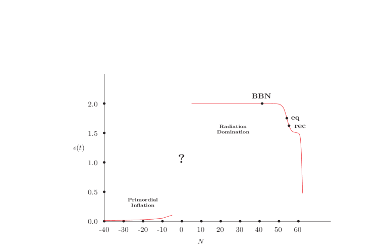
Figure 1: The red curve shows the first slow roll parameter $\epsilon(t)\equiv-\dot{H}/{H^{2}}$ as a function of the number of e-foldings $N$ since the end of primordial inflation. A question mark stands for the phase of reheating between the epochs of primordial inflation and radiation domination, because there are many models for this period. Significant events marked on the graph are Big Bang Nucleosynthesis (BBN) when the seven lightest isotopes were produced, matter-radiation equality (eq) when the energy density was composed of equal amounts of relativistic and non-relativistic matter, and recombination (rec) when neutral Hydrogen formed and the cosmic microwave radiation began free-streaming. Observable cosmological perturbations experience first horizon crossing near the lower left hand corner of the graph.

On scales larger than about 100 Mpc the observable universe is approximately homogeneous, isotropic and spatially flat. The invariant element for such a geometry can be put in the form,

$$ds^{2}=-c^{2}dt^{2}+a^{2}(t)d\vec{x}\!\cdot\!d\vec{x}\;.$$ (1)

Two derivatives of the scale factor $a(t)$ have great significance, the Hubble parameter $H(t)$ and the first slow roll parameter $\epsilon(t)$,

$$H(t)\equiv\frac{\dot{a}}{a}\qquad,\qquad\epsilon(t)\equiv-\frac{\dot{H}}{H^{2}}\;.$$ (2)

Inflation is defined as $H(t)>0$ with $\epsilon(t)<1$. One can see that it is possible from the current values of the cosmological parameters (denoted by a subscript zero) [25],

$$H_{0}\approx 2.2\times 10^{-18}~{}{\rm Hz}\qquad,\qquad\epsilon_{0}\approx 0.47\;.$$ (3)

However, the important phase of inflation for my purposes is Primordial Inflation, which is conjectured to have occurred during the first $10^{-32}$ seconds of existence. If the BICEP2 detection of primordial B-mode polarization is accepted then we finally know the values of $H(t)$ and $\epsilon(t)$ near the end of primordial inflation [26],

$$H_{i}\approx 1.8\times 10^{+38}~{}{\rm Hz}\qquad,\qquad\epsilon_{i}\approx 0.013\;.$$ (4)

I will comment later on the significance of $H_{i}$. Let us here note that $\epsilon_{i}$ is very near the de Sitter limit of $\epsilon=0$ at which the Hubble parameter becomes constant. This is a very common background to use when estimating quantum effects during primordial inflation.

We have direct observational evidence that both the scale factor and its logarithmic time derivative $H(t)$ have changed over many orders of magnitude during cosmic history. In contrast, the deceleration parameter only varies over the small range $0\leq\epsilon(t)\leq 2$. Figure 1 shows what we think we know about $\epsilon(t)$ as a function of the number of e-foldings since the end of primordial inflation at $t=t_{e}$,

$$N(t)\equiv\ln\Bigl{[}\frac{a(t)}{a(t_{e})}\Bigr{]}\;.$$ (5)

It is a tribute to decades of observational work that only a small portion of this figure is really unknown, corresponding to the phase of re-heating at the end of inflation.

Primordial inflation was advanced in the late 1970’s and early 1980’s to explain the absence of observed relics (primordial black holes, magnetic monopoles, cosmic strings) and the initial conditions (homogeneous, isotropic and spatially flat) for the long epoch of radiation domination which is visible on Figure 1. After some notable precursors [27, 28, 29, 30], the paper of Guth [31] focussed attention on the advantages of a early epoch of inflation and, incidentally, coined the name. Important additional work concerned finding an acceptable way to commence inflation and to make it end [32, 33]. The first completely successful model was Linde’s “Chaotic Inflation” [34].

One of the most powerful motivations for primordial inflation is that it explains the Horizon Problem of why events far back in our past light-cone seem so uniform. I will review the argument here because the same analysis is useful for the next subsection. From the cosmological geometry (1) we can easily compute the coordinate distance $R(t_{2},t_{1})$ traversed by a light ray whose trajectory obeys $ds^{2}=0$,

$$R(t_{2},t_{1})\equiv\int_{t_{2}}^{t_{1}}\!\!\!\frac{cdt}{a(t)}\;.$$ (6)

Now note the relation,

$$\frac{d}{dt}\Biggl{[}\frac{1}{(\epsilon\!-\!1)Ha}\Biggr{]}=\frac{1}{a}\Biggl{[}1-\frac{\dot{\epsilon}}{(\epsilon\!-\!1)^{2}H}\Biggr{]}\;.$$ (7)

One can see from Figure 1 that $\epsilon(t)$ was nearly constant over long periods of cosmic evolution, in particular during the epoch of radiation domination, which would extend back to the beginning if it were not for primordial inflation. So we can drop the second term of (7) to conclude,

$$R(t_{2},t_{1})\approx\frac{c}{(\epsilon_{1}\!-\!1)H_{1}a_{1}}-\frac{c}{(\epsilon_{2}\!-\!1)H_{2}a_{2}}\;.$$ (8)

One additional exact relation brings the horizon problem to focus,

$$\frac{d}{dt}\Bigl{[}H(t)a(t)\Bigr{]}=-\Bigl{[}\epsilon(t)\!-\!1\Bigr{]}H^{2}(t)a(t)\;.$$ (9)

Combining equation (9) with (8) reveals a crucial distinction between inflation ($\epsilon(t)<1$) and deceleration ($\epsilon(t)>1$): during deceleration the radius of the light-cone is dominated by its upper limit, whereas the lower limit dominates during inflation. The horizon problem derives from assuming that there was no phase of primordial inflation so that the epoch of radiation domination extends back to the beginning of the universe. Suppose that the universe began at $t=t_{2}$ and we view some early event such as recombination (rec on Fig. 1) or big bang nucleosynthesis (BBN on Fig. 1). At time $t=t_{1}$ we can see things out to the radius of our past light-cone $R(t_{1},t_{0})$ which is vastly larger than the radius of the forward light-cone $R(t_{2},t_{1})\approx c/[(\epsilon_{1}-1)H_{1}a_{1}]$ that anything can have travelled from the beginning of time. For example, the cosmic microwave radiation is uniform to one part in $10^{5}$, which is far better thermal equilibrium than the air of the room in which you are sitting. Without a phase of primordial inflation we are seeing about 2200 different patches of the sky which have not even had time to exchange a single photon, much less achieve a high degree of thermal equilibrium [14]. Of course the problem just gets worse the further back we look. At the time of big bang nucleosynthesis we are seeing about $10^{15}$ causally disconnected regions, which are nonetheless in rough thermal equilibrium [14].

Without inflation the radius $R(t_{2},t_{1})$ of the forward light-cone is almost independent of the beginning of time $t_{2}$. No matter how early we make $t_{2}$ it is not possible to increase $R(t_{2},t_{1})$ more than about $c/[(\epsilon_{1}-1)H_{1}a_{1}]$. Hence the high degree of uniformity we observe in the early universe would have to be a spectacularly unlikely accident. Primordial inflation solves the problem neatly by making the lower limit of the forward light-cone dominate, $R(t_{2},t_{1})\approx c/[(1-\epsilon_{2})H_{2}a_{2}]$. We can make the radius of the forward light-cone much larger than the radius of the past light-cone, so that causal processes would have had plenty of time to achieve the high degree of equilibrium that is observed.

Before closing this subsection I want to return to the numerical values quoted for $H_{0}$ and $H_{i}$ in relations (3-4). The loop counting parameter of quantum gravity can be expressed in terms of the square of the Planck time, $T^{2}_{\rm Pl}\equiv\hbar G/c^{5}\approx 2.9\times 10^{-87}~{}{\rm sec}^{2}$. Quantum gravitational effects from a process whose characteristic frequency is $\omega$ are typically of order $\omega^{2}T^{2}_{\rm Pl}$. For inflationary particle production the characteristic frequency is of course the Hubble parameter, so we can easily compare the strengths of quantum gravitational effects during the current phase of inflation and from the epoch of primordial inflation,

$$\frac{\hbar GH_{0}^{2}}{c^{5}}\approx 1.4\times 10^{-122}\qquad,\qquad\frac{\hbar GH_{i}^{2}}{c^{5}}\approx 9.4\times 10^{-11}\;.$$ (10)

The minuscule first number is why we will never detect quantum gravitational effects from the current phase of inflation. Although the second number is tiny, it is not so small as to preclude detection, if only the signal can persist until the present day. In the next subsection I will explain how that can happen.

The loop counting parameter $\hbar GH^{2}/c^{5}$ is the quantum gravitational analog of the quantum electrodynamic fine structure constant $\alpha\equiv e^{2}/4\pi\epsilon_{0}\hbar c\approx 7.3\times 10^{-3}$. Both parameters control the strength of perturbative corrections. Recall that a result in quantum electrodynamics — for example, the invariant amplitude of Compton scattering — typically consists of a lowest, tree order contribution of strength $\alpha$, then each additional loop brings an extra factor of $\alpha$. In the same way, the lowest, tree order quantum gravity effects from inflationary particle production have strength $\hbar GH^{2}/c^{5}$, and each addition loop brings an extra factor of $\hbar GH^{2}/c^{5}$. Because the quantum gravitational loop counting parameter from primordial inflation is so much smaller than its quantum electrodynamics cousin, we expect that quantum gravitational perturbation theory should be wonderfully accurate. In fact, all that can be resolved with current data is the tree order effect, although I will argue in section 4 that the one loop correction may eventually be resolved. Beyond that there is no hope.

2 Inflationary Particle Production

The phenomenon of polarization in a medium is covered in undergraduate electrodynamics. The medium contains a vast number of bound charges. The application of an electric field makes positive charges move with the field and the negative changes move opposite. That charge separation polarizes the medium and tends to reduce the electric field strength.

One of the amazing predictions of quantum field theory is that virtual particles are continually emerging from the vacuum, existing for a brief period, and then disappearing. How long these virtual particles can exist is controlled by the energy-time uncertainty principle, which gives the minimum time $\Delta t$ needed to resolve and energy difference $\Delta E$,

$$\Delta t\Delta E\mathrel{\raise 1.29167pt\hbox{$>$\kern-7.5pt\lower 4.30554pt\hbox{$\sim$}}}\hbar\;.$$ (11)

If one imagines the emergence of a pair of positive and negatively charged particles of mass $m$ and wave vector $\pm\vec{k}$ then the energy went from zero to $E=2[m^{2}c^{4}+\hbar^{2}c^{2}k^{2}]^{\frac{1}{2}}$. To not resolve a violation of energy conservation, the energy-time uncertainty principle requires the pair to disappear after a time $\Delta t$ given by,

$$\Delta t\sim\frac{\hbar}{\sqrt{m^{2}c^{4}+\hbar^{2}c^{2}k^{2}}}\;.$$ (12)

The rest is an exercise is classical (that is, non-quantum) physics. If we ignore the change in the particles’ momentum then their positions obey,

$$\frac{d^{2}}{cdt^{2}}\Bigl{(}\sqrt{m^{2}c^{2}+\hbar^{2}k^{2}}\,\Delta\vec{x}_{\pm}\Bigr{)}=\pm e\vec{E}\quad\Longrightarrow\quad\Delta\vec{x}_{\pm}(\Delta t)=\frac{\pm\hbar^{2}e\vec{E}}{2c[m^{2}c^{2}+\hbar^{2}k^{2}]^{\frac{3}{2}}}\;.$$ (13)

Hence the polarization induced by wave vector $\vec{k}$ is,

$$\vec{p}=+e\Delta\vec{x}_{+}(\Delta t)-e\Delta\vec{x}_{-}(\Delta t)=\frac{\hbar^{2}e^{2}\vec{E}}{c[m^{2}c^{2}+\hbar^{2}k^{2}]^{\frac{3}{2}}}\;.$$ (14)

The full vacuum polarization density comes from integrating $d^{3}k/(2\pi)^{3}$.

The simple analysis I have just sketched gives pretty nearly the prediction from one loop quantum electrodynamics, which is in quantitative agreement with experiment. It allows us to understand two features of vacuum polarization which would be otherwise obscure:

• That the largest effect derives from the lightest charged particles because they have the longest persistence times $\Delta t$ and therefore induce the greatest polarization; and

• That the electrodynamic interaction becomes stronger at short distances because the longest wave length (hence smallest $k$) virtual particles could induce more polarization than is allowed by the travel time between two very close sources.

Cosmological expansion can strengthen quantum effects because it causes the virtual particles which drive them to persist longer. This is easy to see from the geometry (1). Because spatial translation invariance is unbroken, particles still have conserved wave numbers $\vec{k}$. However, because the physical distance is the coordinate distance scaled by $a(t)$, the physical energy of a particle with mass $m$ and wave number $k=2\pi/\lambda$ becomes time dependent,

$$E(t,\vec{k})=\sqrt{m^{2}c^{4}+\frac{\hbar^{2}c^{2}k^{2}}{a^{2}(t)}}\;.$$ (15)

Hence the relation for the persistence time $\Delta t$ of a virtual pair which emerges at time $t$ changes from (12) to,

$$\int_{t}^{t+\Delta t}\!\!\!\!dt^{\prime}E(t^{\prime},\vec{k})\sim\hbar\;.$$ (16)

Massless particles persist the longest, just as they do in flat space. However, for inflation it is the lower limit of (16) which dominates, so that even taking $\Delta t$ to infinity does not cause the integral to grow past a certain point. One can see this from the de Sitter limit,

$$\int_{t}^{t+\Delta t}\!\!\!\!dt^{\prime}\frac{\hbar ck}{a(t^{\prime})}=\frac{\hbar ck}{H_{i}a(t)}\Bigl{[}1-e^{-H_{i}\Delta t}\Bigr{]}\;.$$ (17)

A particle with $ck<H(t)a(t)$ is said to be super-horizon, and we have just shown that any massless virtual particle which emerges from the vacuum with a super-horizon wave number during inflation will persist forever.

It turns out that almost all massless particles possess a symmetry known as conformal invariance which suppresses the rate at which they emerge from the vacuum. This keeps the density of virtual particles small, even though any that do emerge can persist forever. One can see the problem by specializing the Lagrangian of a massless, conformally coupled scalar $\psi(t,\vec{x})$ to the cosmological geometry (1),

$$\mathcal{L}=-\frac{1}{2}\partial_{\mu}\psi\partial_{\nu}\psi g^{\mu\nu}\sqrt{-g}-\frac{R}{12}\psi^{2}\sqrt{-g}\longrightarrow\frac{a^{3}}{2}\Bigl{[}\frac{\dot{\psi}^{2}}{c^{2}}-\frac{\partial_{i}\psi\partial_{i}\psi}{a^{2}}-\frac{(\dot{H}+2H^{2})\psi^{2}}{c^{2}}\Bigr{]}.$$ (18)

The equation for a canonically normalized, spatial plane wave of the form $\psi(t,\vec{x})=v(t,k)e^{i\vec{k}\cdot\vec{x}}$ can be solved for a general scale factor $a(t)$,

$$\ddot{v}+3H\dot{v}+\Bigl{[}\frac{c^{2}k^{2}}{a^{2}}+\dot{H}+2H^{2}\Bigr{]}v=0\;\Longrightarrow\;v(t,k)=\sqrt{\frac{\hbar}{2ck}}\frac{\exp[-ick\!\int_{t_{i}}^{t}\!\frac{dt^{\prime}}{a(t^{\prime})}]}{a(t)}\;.$$ (19)

The factor of $1/a(t)$ in (19) suppresses the emergence rate, even though destructive interference from the phase dies off, just as the energy-time uncertainty principle (17) predicts. The stress-energy contributed by this field is,

$$T_{\mu\nu}=\Bigl{[}\delta^{\rho}_{\mu}\delta^{\sigma}_{\nu}\!-\!\frac{1}{2}g_{\mu\nu}g^{\rho\sigma}\Bigr{]}\partial_{\rho}\psi\partial_{\sigma}\psi+\frac{1}{6}\Bigl{[}R_{\mu\nu}\!-\!\frac{1}{2}g_{\mu\nu}R\!+\!g_{\mu\nu}\kern 1.0pt\vbox{\hrule height=1.2pt\hbox{\vrule width=1.2pt\hskip 3.0pt\vbox{\vskip 6.0pt}\hskip 3.0pt\vrule width=0.6pt}\hrule height=0.6pt}\kern 1.0pt\!-\!D_{\mu}D_{\nu}\Bigr{]}\psi^{2}\;,$$ (20)

where $D_{\mu}$ is the covariant derivative and        is the covariant d’Alembertian. We can get the 0-point energy of a single wave vector $\vec{k}$ by specializing $T_{00}$ to the cosmological geometry (1) and multipling by a factor of $a^{3}(t)$,

$$\mathcal{E}(t,\vec{k})=\frac{a^{3}}{2}\Bigl{[}|\dot{v}|^{2}+\Bigl{(}\frac{c^{2}k^{2}}{a^{2}}\!+\!H^{2}\Bigr{)}|v|^{2}+H\Bigl{(}v\dot{v}^{*}\!+\!\dot{v}v^{*}\Bigr{)}\Bigr{]}=\frac{\hbar ck}{2a(t)}\;.$$ (21)

This is just the usual $\frac{1}{2}\hbar\omega$ term which is not strengthened but rather weakened by the cosmological expansion.

Only gravitons and massless, minimally coupled scalars are both massless and not conformally invariant so that they can engender significant quantum effects during inflation. Because they obey the same mode equation [35, 36] it will suffice to specialize the scalar Lagrangian to the cosmological geometry (1),

$$\mathcal{L}=-\frac{1}{2}\partial_{\mu}\phi\partial_{\nu}\phi g^{\mu\nu}\sqrt{-g}\longrightarrow\frac{1}{2}a^{3}\Bigl{[}\frac{\dot{\phi}^{2}}{c^{2}}-\frac{1}{a^{2}}\partial_{i}\phi\partial_{i}\phi\Bigr{]}\;.$$ (22)

The equation for a canonically normalized, spatial plane wave of the form $\phi(t,\vec{x})=u(t,k)e^{i\vec{k}\cdot\vec{x}}$ is simpler than that of its conformally coupled cousin (19) but more difficult to solve, so I will specialize the solution to de Sitter,

$$\ddot{u}+3H\dot{u}+\frac{c^{2}k^{2}}{a^{2}}\,u=0\;\Longrightarrow\;u(t,k)=\sqrt{\frac{\hbar}{2ck}}\Bigl{[}1+\frac{iH_{i}a(t)}{ck}\Bigr{]}\frac{\exp[-ick\!\int_{t_{i}}^{t}\!\frac{dt^{\prime}}{a(t^{\prime})}]}{a(t)}\;.$$ (23)

The minimally coupled mode function $u(t,k)$ has the same phase factor as the conformal mode function (19), and they both fall off like $1/a(t)$ in the far sub-horizon regime of $ck\gg H_{i}a(t)$. However, they disagree strongly in the super-horizon regime during which $v(t,k)$ continues to fall off whereas $u(t,k)$ approaches a phase times $H_{i}\sqrt{\hbar/2c^{3}k^{3}}$. One can see from the equation on the left of (23) that $u(t,k)$ approaches a constant for any inflating geometry.

The 0-point energy in wave vector $\vec{k}$ is,

$$\mathcal{E}(t,\vec{k})=\frac{1}{2}a^{3}\Bigl{[}|\dot{u}|^{2}+\frac{c^{2}k^{2}}{a^{2}}|u|^{2}\Bigr{]}=\frac{\hbar ck}{a(t)}\Bigl{[}\frac{1}{2}+\Bigl{(}\frac{H_{i}a(t)}{2ck}\Bigr{)}^{2}\Bigr{]}\;.$$ (24)

Because each wave vector is an independent harmonic oscillator with mass proportional to $a^{3}(t)$ and frequency $k/a(t)$ we can read off the occupation number from expression (24),

$$N(t,\vec{k})=\Bigl{[}\frac{H_{i}a(t)}{2ck}\Bigr{]}^{2}\;.$$ (25)

As one might expect, this number is small in the sub-horizon regime. It becomes of order one at the time $t_{k}$ of horizon crossing, $ck=H(t_{k})a(t_{k})$, and $N(t,\vec{k})$ grows explosively afterwards. This is crucial because it means that inflationary particle production is an infrared effect. That means we can study it reliably using quantum general relativity, even though that theory is not perturbatively renormalizable.

The final point I wish to make is that the mode function $u(t,k)$ becomes constant after first horizon crossing. For de Sitter this constant is calculable,

$$u(t,k)\Biggl{|}_{\rm dS}\longrightarrow iH_{i}\sqrt{\frac{\hbar}{2c^{3}k^{3}}}\exp\Bigl{[}-\frac{ick}{H_{i}a_{i}}\Bigr{]}\;.$$ (26)

However, one can see from the mode equation on the left hand side of (23) that the approach to a constant happens for any inflating geometry. Recall from equation (9) that the inverse horizon length $c^{-1}H(t)a(t)$ grows during inflation and decreases during the later phase of deceleration which encompasses so much of the cosmological history depicted in Figure 1. Hence we can give the following rough summary of the “life cycle of a mode” of wave number $k$:

• At the onset of primordial inflation the mode has $ck\gg H(t)a(t)$ so the mode function oscillates and falls off like $1/a(t)$;

• If inflation lasts long enough the mode will eventually experience first horizon crossing $ck=H(t_{k})a(t_{k})$, after which mode function becomes approximately constant; and

• During the phase of deceleration which follows primordial inflation, modes which experienced first horizon crossing near the end of inflation re-enter the horizon $ck=H(T_{k})a(T_{k})$, after which they begin participating in dynamical processes with amplitude larger by a factor of $a(T_{k})/a(t_{k})$ than they would have had without first horizon crossing.

This is how quantum gravitational effects from the epoch of primordial inflation become fossilized so that they can be detected now.

3 Tree Order Power Spectra

Although the evidence for primordial inflation is overwhelming, there is not yet any compelling mechanism for causing it. The simplest class of successful models is based on general relativity plus a scalar inflaton $\varphi(x)$ whose potential $V(\varphi)$ is regarded as a free function [34],

$$\mathcal{L}=\Bigl{[}\frac{c^{4}\mathbf{R}}{16\pi G}-\frac{1}{2}\varphi_{,\mu}\varphi_{,\nu}\mathbf{g}^{\mu\nu}-V(\varphi)\Bigr{]}\sqrt{-\mathbf{g}}\;.$$ (27)

Here $\mathbf{g}_{\mu\nu}(x)$ is the $D$-dimensional, spacelike metric with Ricci curvature $\mathbf{R}$. (I will work in $D$ spacetime dimensions to facilitate the use of dimensional regularization, even though the $D=4$ limit must eventually be taken for physical results.) The purpose of this section is to show how this simple model can not only drive primordial inflation but also the quantum gravitational fluctuations whose imprint on the cosmic background radiation has been imaged with stunning accuracy [37, 38, 39, 25].

I first demonstrate that the potential $V(\varphi)$ can be chosen to support the cosmological geometry (1) with any scale factor $a(t)$ for which the Hubble parameter is monotonically decreasing. I also comment on the many problems of plausibility which seem to point to the need for a better model. I then decompose perturbations about the background (1) into a scalar $\zeta(x)$ and a transverse-traceless tensor $h_{ij}(x)$. Owing to the particle production mechanism adumbrated in section 2, certain modes of $\zeta$ and $h_{ij}$ become hugely excited during primordial inflation, and then freeze in so that they can survive to much later times. The strength of this effect is quantified by the primordial scalar and tensor power spectra, which I define and compute at tree order, along with associated observables. I then discuss the controversy which has arisen concerning an alternate definition of the tree order power spectra. The section closes with an explanation of why the tree order power spectra are the first quantum gravitational effects ever to have been resolved.

I will adopt the notation employed in recent studies by Maldacena [40] and by Weinberg [20], however, the original work for tensors was done in 1979 by Starobinsky [41], and for scalars in 1981 by Mukhanov and Chibisov [42]. Important subsequent work was done over the course of the next several years by Hawking [43], by Guth and Pi [44], by Starobinsky [45], by Bardeen, Steinhardt and Turner [46], and by Mukhanov [47]. Some classic review articles on the subject are [48, 49, 50].

1 The Background for Single-Scalar Inflation

There is no question that a minimally coupled scalar potential model of the form (27) can support inflation because there is a constructive procedure for finding the potential $V(\varphi)$ given the expansion history $a(t)$ [51, 52, 53, 54]. For the geometry (1) the scalar depends just on time $\varphi_{0}(t)$ and only two of Einstein’s equations are nontrivial,

$$\frac{1}{2}(D\!-\!2)(D\!-\!1)H^{2} = \frac{8\pi G}{c^{2}}\Bigl{[}\frac{\dot{\varphi}^{2}_{0}}{c^{2}}+V(\varphi_{0})\Bigr{]}\;,$$ (28)

$$-(D\!-\!2)\dot{H}-\frac{1}{2}(D\!-\!2)(D\!-\!1)H^{2} = \frac{8\pi G}{c^{2}}\Bigl{[}\frac{\dot{\varphi}^{2}_{0}}{c^{2}}-V(\varphi_{0})\Bigr{]}\;.$$ (29)

By adding (28) and (29) one obtains the relation,

$$(D\!-\!2)\dot{H}=\frac{8\pi G}{c^{4}}\,\dot{\varphi}^{2}_{0}\;.$$

Hence one can reconstruct the scalar’s evolution provided the Hubble parameter is monotonically decreasing, and that relation can be inverted (numerically if need be) to solve for time as a function of

$$\varphi_{0}(t)=\varphi_{0}(t_{2})\pm\int_{t_{2}}^{t}\!\!dt^{\prime}\sqrt{\frac{-(D\!-\!2)c^{4}\dot{H}(t^{\prime})}{8\pi G}}\qquad\Longleftrightarrow\qquad t=T(\varphi_{0})\;.$$ (30)

One then determines the potential by subtracting (29) from (28) and evaluating the resulting function of time at $t=T(\varphi_{0})$,

$$V(\varphi_{0})=\frac{(D\!-\!2)c^{2}}{16\pi G}\Biggl{[}\dot{H}\Bigl{(}T(\varphi_{0})\Bigr{)}+3H^{2}\Bigl{(}T(\varphi_{0})\Bigr{)}\Biggr{]}\;.$$ (31)

Just because scalar potential models (27) can be adjusted to work does not mean they are particularly plausible. They suffer from six sorts of sometimes contradictory fine-tuning problems:

1. Initial Conditions — Inflation must begin with the inflaton approximately homogeneous, and potential-dominated, over more than a Hubble volume [55];

2. Duration — The inflaton potential must be flat enough to make inflation last for at least 50 e-foldings [32, 33];

3. Scalar Perturbations — Getting the right magnitude for the scalar power spectrum requires $\hbar G^{3}/c^{11}\times V^{3}/{V^{\prime}}^{2}\sim 10^{-11}$ [48];

4. Tensor Perturbations — Getting the right magnitude for the tensor power spectrum requires $c^{4}/G\times(V^{\prime}/V)^{2}\sim 1$ [48];

5. Reheating — The inflaton must couple to ordinary matter (its gravitational couplings do not suffice) so that its post-inflationary kinetic energy produces a hot, radiation dominated universe [56];

6. Cosmological Constant — The minimum of the scalar potential must have the right value $\hbar G^{2}V_{\rm min}/c^{7}\approx 10^{-123}$ to contribute the minuscule vacuum energy we observe today [57, 58, 59, 60].

Note that adding the matter couplings required to produce reheating puts 2-4 at risk because matter loop effects induce Coleman-Weinberg corrections to the inflaton effective potential. Nor does fundamental theory provide any explanation for why the cosmological constant is so small [61, 62]. The degree of fine-tuning needed to enforce these six conditions strains credulity, and disturbs even those who devised the early models [63, 64, 65, 66].

Opinions differ, but I feel it is a mistake to make too much of the defects of single-scalar inflation. The evidence for an early phase of accelerated expansion is overwhelming and really incontrovertible, irrespective of what caused it. Further, all that we know about low energy effective field theory confirms that the general relativity portion of Lagrangian (27) must be valid, even at the scales of primordial inflation. That suffices to establish the quantum gravitational character of primordial perturbations, even without a compelling model for what caused inflation. So I will go forward with the analysis on the basis of the single-scalar model (27), firm in the belief that whatever eventually supplants it must exhibit many of the same features.

2 Gauge-Fixed, Constrained Action

We decompose $\mathbf{g}_{\mu\nu}$ into lapse, shift and spatial metric according to Arnowitt, Deser and Misner (ADM) [67, 68, 69],

$$\mathbf{g}_{\mu\nu}dx^{\mu}dx^{\nu}=-N^{2}c^{2}dt^{2}+g_{ij}(dx^{i}\!-\!N^{i}cdt)(dx^{j}\!-\!N^{j}cdt)\;.$$ (32)

ADM long ago showed that the Lagrangian has a very simple dependence upon the lapse [67, 68, 69],

$$\mathcal{L}=\Bigl{(}{\rm Surface\ Terms}\Bigr{)}-\frac{c^{4}\sqrt{g}}{16\pi G}\Bigl{[}N\cdot A+\frac{B}{N}\Bigr{]}\;.$$ (33)

The quantity $A$ is a potential energy,

$$A=-R+\frac{16\pi G}{c^{4}}\Bigl{[}V(\varphi)+\frac{1}{2}\varphi_{,i}\varphi_{,j}g^{ij}\Bigr{]}\;,$$ (34)

where $R$ is the $(D-1)$-dimensional Ricci scalar formed from $g_{ij}$. The quantity $B$ in (33) is a sort of kinetic energy,

$$B=(E^{i}_{~{}i})^{2}-E^{ij}E_{ij}-\frac{8\pi G}{c^{4}}\Bigl{(}\frac{\dot{\varphi}}{c}-\varphi_{,i}N^{i}\Bigr{)}^{2}\;,$$ (35)

where $E_{ij}/N$ is the extrinsic curvature,

$$E_{ij}\equiv\frac{1}{2}\Bigl{[}N_{i;j}+N_{j;i}-c^{-1}\dot{g}_{ij}\Bigr{]}\;,$$ (36)

and a semi-colon denotes spatial covariant differentiation using the connection compatible with $g_{ij}$.

ADM fix the gauge by specifying $N(t,\vec{x})$ and $N^{i}(t,\vec{x})$, however, Maldacena [40] and Weinberg [20] instead impose the conditions,

$$G_{0}(t,\vec{x}) \equiv \varphi(t,\vec{x})-\varphi_{0}(t)=0\;,$$ (37)

$$G_{i}(t,\vec{x}) \equiv \partial_{j}h_{ij}(t,\vec{x})=0\;.$$ (38)

The transverse-traceless graviton field $h_{ij}(t,\vec{x})$ is defined by decomposing the spatial metric into a conformal part and a unimodular part $\widetilde{g}_{ij}$,

$$g_{ij}=a^{2}(t)e^{2\zeta(t,\vec{x})}\widetilde{g}_{ij}(t,\vec{x})\;\Longrightarrow\;\sqrt{g}=a^{D-1}e^{(D-1)\zeta}\;.$$ (39)

The unimodular part is obtained by exponentiating the transverse-traceless graviton field $h_{ij}(t,\vec{x})$,

$$\widetilde{g}_{ij}\equiv\Bigl{[}e^{h}\Bigr{]}_{ij}=\delta_{ij}+h_{ij}+\frac{1}{2}h_{ik}h_{jk}+O(h^{3})\qquad,\qquad h_{ii}=0\;.$$ (40)

The Faddeev-Popov determinant associated with (37-38) depends only on $h_{ij}$, and becomes singular for $\epsilon=0$.

Of course no gauge can eliminate the physical scalar degree of freedom which is evident in (27). With condition (37) the inflaton degree of freedom resides in $\zeta(t,\vec{x})$ and linearized gravitons are carried by $h_{ij}(t,\vec{x})$. In this gauge the lapse and shift are constrained variables which mediate important interactions between the dynamical fields but contribute no independent degrees of freedom. Varying (33) with respect to $N$ produces an algebraic equation for $N$,

$$A-\frac{B}{N^{2}}=0\qquad\Longrightarrow\qquad N=\sqrt{\frac{B}{A}}\;$$ (41)

This gives the constrained Lagrangian a “virial” form [70],

$$\mathcal{L}_{\rm const}=\Bigl{(}{\rm Surface\ Terms}\Bigr{)}-\frac{c^{4}\sqrt{g}}{8\pi G}\,\sqrt{AB}\;.$$ (42)

From relations (1-30) one can see that the background values of the potential and kinetic terms are equal, $A_{0}=B_{0}=(D\!-\!2)c^{-2}[\dot{H}+(D\!-\!1)H^{2}]$. Hence the background value of the lapse is unity.

There is unfortunately no nonperturbative solution for the shift $N^{i}(t,\vec{x})$ in terms of $\zeta$ and $h_{ij}$, so its constraint equation must be solved perturbatively. One first employs (39) to exhibit how the potential (34) depends on $\zeta$ and $h_{ij}$,

$$A=A_{0}-R\equiv A_{0}(1+\alpha)\;.$$ (43)

Here the spatial Ricci scalar is,

$$R=\frac{e^{-2\zeta}}{a^{2}}\Biggl{[}\widetilde{R}-2(D\!-\!2)\widetilde{\nabla}^{2}\zeta-(D\!-\!2)(D\!-\!3)\zeta^{,k}\widetilde{g}^{k\ell}\zeta_{,\ell}\Biggr{]}\;,$$ (44)

where $\widetilde{R}=O(h^{2})$ is the Ricci scalar formed from $\widetilde{g}_{ij}$ and $\widetilde{\nabla}^{2}\equiv\partial_{i}\widetilde{g}^{ij}\partial_{j}$ is the conformal scalar Laplacian. The full scalar Laplacian is,

$$\nabla^{2}\equiv\frac{1}{\sqrt{g}}\partial_{i}\Bigl{[}\sqrt{g}\,g^{ij}\partial_{j}\Bigr{]}\;.$$ (45)

At this stage one can recognize that the dimensionless 3-curvature perturbation $\mathcal{R}$ is just $\zeta$, in $D=4$ dimensions and to linearized order [49],

$$\mathcal{R}(t,\vec{x})\equiv-\frac{1}{4\nabla^{2}}\,R=\Bigl{(}\frac{D\!-\!2}{2}\Bigr{)}\zeta(t,\vec{x})+O\Bigl{(}\zeta^{2},\zeta h,h^{2}\Bigr{)}\;.$$ (46)

The kinetic energy (35) can be expressed as,

$$B\equiv A_{0}(1\!+\!\beta)=A_{0}+2(D\!-\!2)c^{-1}H\Bigl{[}(D\!-\!1)(c^{-1}\dot{\zeta}\!-\!\zeta_{,k}\widetilde{N}^{k})\!-\!\widetilde{N}^{k}_{~{},k}\Bigr{]}-\widetilde{E}^{k\ell}\widetilde{E}_{k\ell}$$ (47)

$$\hskip 14.22636pt+(D\!-\!2)(D\!-\!1)\Bigl{(}\frac{\dot{\zeta}}{c}\!-\!\zeta_{,k}\widetilde{N}^{k}\Bigr{)}^{2}\!\!\!-2(D\!-\!2)\Bigl{(}\frac{\dot{\zeta}}{c}\!-\!\zeta_{,k}\widetilde{N}^{k}\Bigr{)}\widetilde{N}^{k}_{~{},k}+(\widetilde{N}^{k}_{~{},k})^{2}\;.\qquad$$

Here we define $\widetilde{N}^{i}\equiv N^{i}$, $\widetilde{N}_{i}\equiv\widetilde{g}_{ij}\widetilde{N}^{j}$ and $\widetilde{E}_{ij}\equiv\frac{1}{2}[\widetilde{N}_{i;j}+\widetilde{N}_{j;i}-c^{-1}\dot{h}_{ij}]$.

The next step is to expand the volume part of the constrained Lagrangian in powers of $\alpha$ and $\beta$,

$$-\frac{c^{4}\sqrt{g}}{8\pi G}\,\sqrt{AB} = -\frac{c^{4}a^{D-1}e^{(D-1)\zeta}}{8\pi G}\,A_{0}\sqrt{(1\!+\!\alpha)(1+\beta)}\;,$$ (48)

$$= -\frac{c^{4}a^{D-1}e^{(D-1)\zeta}}{8\pi G}\,A_{0}\Biggl{\{}1\!+\!\frac{(\alpha\!+\!\beta)}{2}\!-\!\frac{(\alpha\!-\!\beta)^{2}}{8}\!+\!\dots\Biggr{\}}.\qquad$$ (49)

As Weinberg noted, the terms involving no derivatives of $\zeta$ or $h_{ij}$ sum up to a total derivative [20],

$$a^{D-1}A_{0}=\frac{\partial}{\partial t}\Bigl{[}(D\!-\!2)Ha^{D-1}\Bigr{]}\;.$$ (50)

Another important fact is that quadratic mixing between $\widetilde{N}^{i}$ and $\zeta$ can be eliminated with the covariant field redefinition [70],

$$\widetilde{S}^{k}\equiv\widetilde{N}^{k}+\widetilde{g}^{k\ell}\partial_{\ell}\frac{1}{\widetilde{\nabla}^{2}}\Bigl{[}\frac{ce^{-2\zeta}}{Ha^{2}}\widetilde{\nabla}^{2}\zeta-\epsilon(c^{-1}\dot{\zeta}\!-\!\zeta_{,i}\widetilde{N}^{i})\Bigr{]}\;.$$ (51)

After much work the quadratic Lagrangians emerge,

$$\mathcal{L}_{S^{2}} \!=\! \frac{c^{4}a^{D-1}}{32\pi G}\Biggl{\{}\partial_{\ell}\widetilde{S}^{k}\partial_{\ell}\widetilde{S}^{k}\!\!+\!\Bigl{(}\frac{D\!-\!3\!+\!\epsilon}{D\!-\!1\!-\!\epsilon}\Bigr{)}\partial_{\ell}\widetilde{S}^{k}\partial_{k}\widetilde{S}^{\ell}\Biggr{\}}\;,\qquad$$ (52)

$$\mathcal{L}_{\zeta^{2}} \!=\! \frac{(D\!-\!2)c^{4}\epsilon\,a^{D-1}}{16\pi G}\Biggl{\{}\frac{\dot{\zeta}^{2}}{c^{2}}-\frac{\partial_{k}\zeta\partial_{k}\zeta}{a^{2}}\Biggr{\}},$$ (53)

$$\mathcal{L}_{h^{2}} \!=\! \frac{c^{4}a^{D-1}}{64\pi G}\Biggl{\{}\frac{\dot{h}_{ij}\dot{h}_{ij}}{c^{2}}-\frac{\partial_{k}h_{ij}\partial_{k}h_{ij}}{a^{2}}\Bigr{\}}.$$ (54)

These results suffice for the analysis of this section. To consider loop corrections (or non-Gaussiantity) one must solve the constraint equation for $\widetilde{S}^{i}$,

$$\partial_{j}\partial_{j}\widetilde{S}^{i}+\Bigl{(}\frac{D\!-\!3\!+\!\epsilon}{D\!-\!1\!-\!\epsilon}\Bigr{)}\partial_{i}\partial_{j}\widetilde{S}^{j}=O\Bigl{(}\zeta^{2},\zeta h,h^{2},S\zeta\Bigr{)}\;.$$ (55)

That is a tedious business which has only been carried out to a few orders. I will review what is known in section 1.

3 Tree Order Power Spectra

As we will see in section 3, there is not yet general agreement on how to define the primordial power spectra when loop corrections are included [22, 23]. At tree order we can dispense with dimensional regularization, and also forget about the distinction between $\zeta$ and the dimensionless 3-curvature perturbation (46). The following definitions suffice:

$$\Delta^{2}_{\mathcal{R}}(k,t) \equiv \frac{k^{3}}{2\pi^{2}}\int\!\!d^{3}x\,e^{-i\vec{k}\cdot\vec{x}}\Bigl{\langle}\Omega\Bigl{|}\zeta(t,\vec{x})\zeta(t,\vec{0})\Bigr{|}\Omega\Bigr{\rangle}\;,$$ (56)

$$\Delta^{2}_{h}(k,t) \equiv \frac{k^{3}}{2\pi^{2}}\int\!\!d^{3}x\,e^{-i\vec{k}\cdot\vec{x}}\Bigl{\langle}\Omega\Bigl{|}h_{ij}(t,\vec{x})h_{ij}(t,\vec{0})\Bigr{|}\Omega\Bigr{\rangle}\;.$$ (57)

Although it is useful to retain the time dependence in expressions (56-57), the actual predictions of primordial inflation are obtained by evaluating the time-dependent power spectra safely between the first and second horizon crossing times $t_{k}$ and $T_{k}$ described in section 2,

$$\Delta^{2}_{\mathcal{R}}(k)\equiv\Delta^{2}_{\mathcal{R}}(k,t)\Bigl{|}_{t_{k}\ll t\ll T_{k}}\qquad,\qquad\Delta^{2}_{h}(k)\equiv\Delta^{2}_{h}(k,t)\Bigl{|}_{t_{k}\ll t\ll T_{k}}\;.$$ (58)

The state $|\Omega\rangle$ in expressions (56-57) is annihilated by $\alpha(\vec{k})$ and $\beta(\vec{k},\lambda)$ in the free field expansions of $\zeta$ and $h_{ij}$,

$$\zeta(t,\vec{x}) = \int\!\!\frac{d^{3}k}{(2\pi)^{3}}\Biggl{\{}v(t,k)e^{i\vec{k}\cdot\vec{x}}\alpha(\vec{k})+v^{*}(t,k)e^{-i\vec{k}\cdot\vec{x}}\alpha^{\dagger}(\vec{k})\Biggr{\}}\;,\qquad$$ (59)

$$h_{ij}(t,\vec{x}) = \int\!\!\frac{d^{3}k}{(2\pi)^{3}}\sum_{\lambda=\pm}\Biggl{\{}u(t,k)e^{i\vec{k}\cdot\vec{x}}\epsilon_{ij}(\vec{k},\lambda)\beta(\vec{k},\lambda)+{\rm Conjugate}\Biggr{\}}\;.\qquad$$ (60)

The polarization tensors $\epsilon_{ij}(\vec{k},\lambda)$ are the same as those of flat space. If we adopt the usual normalizations for the creation and annihilation operators,

$$\Bigl{[}\alpha(\vec{k}),\alpha^{\dagger}(\vec{k}^{\prime})\Bigr{]}=(2\pi)^{3}\delta^{3}(\vec{k}\!-\!\vec{k}^{\prime})\quad,\quad\Bigl{[}\beta(\vec{k},\lambda),\alpha^{\dagger}(\vec{k}^{\prime},\lambda^{\prime})\Bigr{]}=\delta_{\lambda\lambda^{\prime}}(2\pi)^{3}\delta^{3}(\vec{k}\!-\!\vec{k}^{\prime})\;.$$ (61)

then canonical quantization of the free Lagrangians (53-54) implies that the mode functions obey,

$$\ddot{v}+\Bigl{[}3H\!+\!\frac{\dot{\epsilon}}{\epsilon}\Bigr{]}\dot{v}+\frac{c^{2}k^{2}}{a^{2}}v=0 v\dot{v}^{*}-\dot{v}v^{*}=\frac{i4\pi\hbar G}{c^{2}\epsilon a^{3}}\;,$$ , (62)

$$\ddot{u}+3H\dot{u}+\frac{c^{2}k^{2}}{a^{2}}u=0 u\dot{u}^{*}-\dot{u}u^{*}=\frac{i32\pi\hbar G}{c^{2}a^{3}}\;.$$ , (63)

It has long been known that the graviton mode function $u(t,k)$ obeys the same equation (23) as that of a massless, minimally coupled scalar [35, 36]. Only their normalizations differ by the square root of $32\pi G/c^{2}$.

By substituting the free field expansions (59-60) into the definitions (56-57) of the power spectra, and then making use of the canonical commutation relations (61), one can express the tree order power spectra in terms of scalar and tensor mode functions,

$$\Delta^{2}_{\mathcal{R}}(k,t) = \frac{k^{3}|v(,kt)|^{2}}{2\pi^{2}}\;,$$ (64)

$$\Delta^{2}_{h}(k,t) = \frac{k^{3}|u(t,k)|^{2}}{2\pi^{2}}\sum_{\lambda=\pm}\epsilon_{ij}\epsilon_{ij}^{*}=\frac{k^{3}|u(k,t)|^{2}}{\pi^{2}}\;.$$ (65)

One of the frustrating things about primordial inflation is that we don’t know what $a(t)$ is so we need results which are valid for any reasonable expansion history. This means that even tree order expressions such as (64-65) can only be evaluated approximately because there are no simple expressions for the mode functions for a general scale factor $a(t)$ [71, 72, 73].

One common approximation is setting $\epsilon(t)$ to a constant, the reliability of which can be gauged by studying the region (at $N\approx-40$) of Figure 1 at which currently observable perturbations freeze in. (The necessity of nonconstant $\epsilon(t)$ later is not relevant for the validity of assuming constant $\epsilon(t)$ to estimate the amplitude at freeze-in.) For constant $\epsilon(t)$ both mode functions are proportional to a Hankel function of the first kind,

$$\dot{\epsilon}=0\qquad\Longrightarrow\qquad v(t,k)=\frac{u(t,k)}{\sqrt{8\epsilon}}\;,$$ (67)

$$u(t,k)=\sqrt{\frac{8\pi^{2}\hbar G}{(1\!-\!\epsilon)c^{2}H(t)a^{3}(t)}}\,H^{(1)}_{\nu}\Bigl{(}\frac{ck}{(1\!-\!\epsilon)H(t)a(t)}\Bigr{)}\;,\;\nu=\frac{1}{2}\Bigl{(}\frac{3\!-\!\epsilon}{1\!-\!\epsilon}\Bigr{)}\;.\qquad$$

Between first and second horizon crossing ($t_{k}\ll t\ll T_{k}$) we can take the small argument limit of the Hankel function,

$$\dot{\epsilon}(t)=0\quad,\quad t_{k}\ll t\ll T_{k}$$ (69)

$$\Longrightarrow u(t,k)\approx\sqrt{\frac{8\pi^{2}\hbar G}{(1\!-\!\epsilon)c^{2}H(t)a^{3}(t)}}\times\frac{-i\Gamma(\nu)}{\pi}\Bigl{[}\frac{2(1\!-\!\epsilon)H(t)a(t)}{ck}\Bigr{]}^{\nu}\;,\qquad$$

$$\hskip 28.45274pt=\sqrt{\frac{16\pi^{2}\hbar G}{c^{5}k^{3}}}\times\frac{-i\Gamma(\nu)}{\pi}\Bigl{[}\frac{2(1\!-\!\epsilon)H(t)a^{\epsilon}(t)}{(ck)^{\epsilon}}\Bigr{]}^{\frac{1}{1-\epsilon}}\;.\qquad$$

Constant $\epsilon(t)$ also implies $H(t)a^{\epsilon}(t)$ is a constant, which we may as well evaluate at the time of first horizon crossing, $H(t)a^{\epsilon}(t)=H^{1-\epsilon}(t_{k})(ck)^{\epsilon}$. With the doubling formula ($\Gamma(2x)=2^{2x-1}/\sqrt{\pi}\times\Gamma(x)\Gamma(x+\frac{1}{2})$) we at length obtain,

$$\dot{\epsilon}(t)=0\quad,\quad t_{k}\ll t\ll T_{k}$$ (70)

$$\Longrightarrow u(t,k)\approx-i\Bigl{[}\frac{1\!-\!\epsilon}{2^{\epsilon}}\Bigr{]}^{\frac{1}{1-\epsilon}}\frac{\Gamma(\frac{2}{1-\epsilon})}{\Gamma(\frac{1}{1-\epsilon})}\times\sqrt{\frac{16\pi\hbar GH^{2}(t_{k})}{c^{5}k^{3}}}\;.\qquad$$

The factor multiplying the square root has nearly unit modulus for small $\epsilon$ — and the BICEP2 result is $\epsilon_{i}=0.013$ [26], while previous data sets give the even smaller bound of $\epsilon_{i}<0.007$ at $95\%$ confidence [37, 38, 39]. Hence it should be reliable to drop this factor, resulting in the approximate forms,

$$\Delta^{2}_{\mathcal{R}}(k)\approx\frac{\hbar GH^{2}(t_{k})}{\pi c^{5}\epsilon(t_{k})}\qquad,\qquad\Delta^{2}_{h}(k)\approx\frac{16\hbar GH^{2}(t_{k})}{\pi c^{5}}\;.$$ (71)

The WKB approximation is another common technique for estimating the freeze-in amplitudes of $v(t,k)$ and $u(t,k)$ which appear in expressions (64-65) for the tree order power spectra. Recall that the method applies to differential equations of the form $\ddot{f}+\omega^{2}(t)f=0$. From expression (63) one can see that reaching this form for the tensor mode function requires the rescaling $f(t,k)=a^{\frac{3}{2}}(t)\times u(t,k)$. It is then simple to recognize the correctly normalized WKB solution and its associated frequency as,

$$u(t,k) \approx \sqrt{\frac{16\pi\hbar G}{c^{2}a^{3}(t)|\omega(t,k)|}}\exp\Biggl{[}-i\!\!\int_{t_{2}}^{t}\!\!dt^{\prime}\omega(t^{\prime},k)\Biggr{]}\;,\qquad$$ (72)

$$\omega^{2}(t,k) \equiv \frac{c^{2}k^{2}}{a^{2}(t)}-\Bigl{[}\frac{9}{4}\!-\!\frac{3}{2}\epsilon(t)\Bigr{]}H^{2}(t)\;.$$ (73)

In the sub-horizon regime of $ck\gg H(t)a(t)$ the frequency is real $\omega(t,k)\approx ck/a(t)$ and the solution (72) both oscillates and falls off like $1/a(t)$. Freeze-in occurs in the super-horizon regime of $ck\ll H(t)a(t)$ during which the frequency is imaginary $\omega(t,k)\approx iH(t)[\frac{3}{2}-\frac{1}{2}\epsilon(t)]$. We can estimate the freeze-in amplitude by computing the real part of the exponent,

$$-i\!\!\int_{t_{k}}^{t}\!\!dt^{\prime}\omega(t^{\prime},k)\approx\int_{t_{k}}^{t}\!\!dt^{\prime}\Biggl{\{}\frac{3}{2}\frac{\dot{a}(t^{\prime})}{a(t^{\prime})}+\frac{1}{2}\frac{\dot{H}(t^{\prime})}{H(t^{\prime})}\Biggr{\}}=\ln\Biggl{[}\frac{a^{\frac{3}{2}}(t)H^{\frac{1}{2}}(t)}{a^{\frac{3}{2}}(t_{k})H^{\frac{1}{2}}(t_{k})}\Biggr{]}\;.$$ (74)

Substituting (74) in (72) and using $H(t_{k})a(t_{k})=ck$ gives the following result for the freeze-in modulus,

$$t_{k}\ll t\ll T_{k}\qquad\Longrightarrow\qquad\Bigl{|}u(t,k)\Bigr{|}_{\rm WKB}\approx\sqrt{\frac{16\pi\hbar GH^{2}(t_{k})}{c^{5}k^{3}|\frac{3}{2}\!-\!\frac{1}{2}\epsilon(t)|}}\;.$$ (75)

If we drop the order one factor of $|\frac{3}{2}-\frac{1}{2}\epsilon(t)|$ the result is (71).

From expression (62) we see that reaching the WKB form for the scalar mode function requires the rescaling $f(t,k)=\epsilon^{\frac{1}{2}}(t)\times a^{\frac{3}{2}}(t)\times v(t,k)$. Its frequency is simpler to express if I first introduce the (Hubble form of the) second slow roll parameter $\eta(t)$,

$$\eta(t)\equiv\epsilon(t)-\frac{\dot{\epsilon}(t)}{2H(t)\epsilon(t)}\;.$$ (76)

The correctly normalized WKB approximation for the scalar mode function and its frequency is,

$$v(t,k) \approx \sqrt{\frac{2\pi\hbar G}{c^{2}\epsilon(t)a^{3}(t)|\nu(t,k)|}}\exp\Biggl{[}-i\!\!\int_{t_{2}}^{t}\!\!dt^{\prime}\nu(t^{\prime},k)\Biggr{]}\;,\qquad$$ (77)

$$\nu^{2}(t,k) \equiv \frac{c^{2}k^{2}}{a^{2}(t)}-\Bigl{[}\Bigl{(}\frac{3}{2}\!+\!\epsilon(t)\!-\!\eta(t)\Bigr{)}\Bigl{(}\frac{3}{2}\!-\!\eta(t)\Bigr{)}+\frac{\dot{\epsilon}\!-\!\dot{\eta}}{H(t)}\Bigr{]}H^{2}(t)\;.\qquad$$ (78)

Freeze-in occurs as one evolves from the sub-horizon regime of $\nu(t,k)\approx ck/a(t)$ to the super-horizon regime of $\nu(t,k)\approx iH(t)[\frac{3}{2}+\frac{1}{2}\epsilon(t)-\eta(t)]$. The real part of the exponent of (77) is,

$$-i\!\!\int_{t_{k}}^{t}\!\!dt^{\prime}\nu(t^{\prime},k)\approx\!\!\int_{t_{k}}^{t}\!\!dt^{\prime}\Biggl{\{}\frac{3}{2}\frac{\dot{a}(t^{\prime})}{a(t^{\prime})}+\frac{1}{2}\frac{\dot{H}(t^{\prime})}{H(t^{\prime})}+\frac{1}{2}\frac{\dot{\epsilon}(t^{\prime})}{\epsilon(t^{\prime})}\Biggr{\}}=\ln\Biggl{[}\frac{a^{\frac{3}{2}}(t)H^{\frac{1}{2}}(t)\epsilon^{\frac{1}{2}}(t)}{a^{\frac{3}{2}}(t_{k})H^{\frac{1}{2}}(t_{k})\epsilon^{\frac{1}{2}}(t_{k})}\Biggr{]}.$$ (79)

Substituting in (77) gives a freeze-in modulus which is again roughly consistent with (71),

$$t_{k}\ll t\ll T_{k}\qquad\Longrightarrow\qquad\Bigl{|}v(t,k)\Bigr{|}_{\rm WKB}\approx\sqrt{\frac{2\pi\hbar GH^{2}(t_{k})}{c^{5}k^{3}\epsilon(t_{k})|\frac{3}{2}\!+\!\frac{1}{2}\epsilon(t)\!-\!\eta(t)|}}\;.$$ (80)

It should be obvious from the discordant factors of order one in expressions (70), (75) and (80), that the results (71) for the tree order power spectra are only approximate. This is confirmed by numerical integration of explicit models [74, 75]. In addition to order one factors depending on the geometry at $t=t_{k}$ there is also a nonlocal “memory factor” which depends on the precise manner in which the mode evolves up to first horizon crossing [73]. Most of the ambiguity derives from not having a definitive model for what caused inflation. Once the expansion history is known it is possible to derive wonderfully accurate results by numerically integrating either the mode functions [76]. It is even more efficient to numerically evolve the time-dependent power spectra directly, without the irrelevant phase information [77].

The tree order power spectra (58) give the tensor-to-scalar ratio $r(k)$, the scalar spectral index $n_{s}(k)$, and the tensor spectral index $n_{t}(k)$,

$$r(k) \equiv \frac{\Delta^{2}_{h}(k)}{\Delta^{2}_{\mathcal{R}}(k)}\approx 16\epsilon(t_{k})\;,$$ (81)

$$n_{s}(k) \equiv 1+\frac{\partial\ln(\Delta^{2}_{\mathcal{R}}(k)}{\partial\ln(k)}\approx 1-4\epsilon(t_{k})+2\eta(t_{k})\;.$$ (82)

$$n_{t}(k) \equiv \frac{\partial\ln(\Delta^{2}_{h}(k)}{\partial\ln(k)}\approx-2\epsilon(t_{k})\;.$$ (83)

In each case the definition is exact, and the approximate result derives from expressions (71) with an additional approximation to relate $dk$ to $dt_{k}$,

$$cdk=[1\!-\!\epsilon(t_{k})]H^{2}(t_{k})a(t_{k})dt_{k}\approx ck\times H(t_{k})dt_{k}\;.$$ (84)

Comparison of (81) and (83) implies an important test on single-scalar inflation which is violated in more general models [78, 79, 80],

$$r\approx-8n_{t}\;.$$ (85)

Certain general trends are also evident from the approximate results (71):

• $r<1$ because $\epsilon\ll 1$;

• $n_{t}<0$ because $H(t)$ decreases; and

• $n_{s}-1<n_{t}$ because $\epsilon(t)$ tends to increase.

To anyone who works in quantum gravity it is breath-taking that we have any data, so it seems petulant to complain that the some of the parameters, and particularly their dependences upon $k$, are still poorly constrained. The scalar power spectrum can be inferred from the measurements of the intensity and the $E$-mode of polarization in cosmic microwave radiation which originates at the time of recombination (rec on Figure 1) and then propagates through the fossilized metric perturbations left over from the epoch of primordial inflation. The latest full-sky results come from the Planck satellite and are fit to the form [25],

$$\Delta^{2}_{\mathcal{R}}(k)\approx A_{s}\Bigl{(}\frac{k}{k_{0}}\Bigr{)}^{n_{s}-1+\frac{dn_{s}}{d\ln(k)}\ln(\frac{k}{k_{0}})}\;.$$ (86)

The fiducial wave number is $k_{0}=0.050~{}{\rm Mpc}^{-1}$, and the quantities “$n_{s}$” and “$dn_{s}/d\ln(k)$” are the scalar spectral index and its derivative evaluated at $k=k_{0}$. When combined with the polarization data from the WMAP satellite [37] the Planck team reports [25],

$$10^{9}\times A_{s}=2.196^{+0.051}_{-0.060}\;,\;n_{s}=0.9603\pm 0.0073\;,\;\frac{dn_{s}}{d\ln(k)}=-0.013\pm 0.018\;.$$ (87)

The tensor-to-scalar ratio is reported at a much smaller wave number of $k=0.002~{}{\rm Mpc}^{-1}$. Bounds on $r_{0.002}$ can be derived from analyzing how the intensity and the $E$-mode of polarization of the cosmic microwave background radiation depend upon $k$. Because this sort of $k$ dependence might also indicate “running” of the scalar spectral index ($dn_{s}/d\ln(k)\neq 0$) the limits on $r_{0.002}$ become significantly weaker if one allows for running. Combining Planck and previous data sets gives the following bounds at $95\%$ confidence [25],

$$r_{0.002} < 0.11\qquad\frac{dn_{s}}{d\ln(k)}=0\;,$$ (88)

$$r_{0.002} < 0.26\qquad\frac{dn_{s}}{d\ln(k)}\neq 0\;.$$ (89)

Direct detection requires a measurement of the $B$-mode of polarization. The BICEP2 team have done this and they report a result consistent with,

$$r_{0.002}\approx 0.20\;.$$ (90)

Although the tensor power spectrum is still poorly known, and controversial [81, 82], resolving it is terrifically important because it tests single-scalar inflation through relation (85) and incidentally fixes the scale of primordial inflation. If only $\Delta^{2}_{\mathcal{R}}(k)$ is resolved one can always construct a single-scalar potential $V(\varphi)$ which will explain it. To see this, suppose we have measured the scalar power spectrum for some range of wave numbers $k_{2}<k<k_{1}$ and use the approximate formula (71), along with the small $\epsilon$ relation (84) between $dt_{k}$ and $dk$, to reconstruct the inflationary Hubble parameter,

$$\frac{1}{H^{2}(t_{k})}-\frac{1}{H^{2}_{2}}=\frac{2\hbar G}{\pi c^{5}}\!\!\int_{k_{2}}^{k}\!\frac{dk^{\prime}}{k^{\prime}\,\Delta^{2}_{\mathcal{R}}(k^{\prime})}\;.$$ (91)

The Hubble parameter $H_{2}\equiv H(t_{2})$ is an integration constant which we can choose to make the tensor power spectrum smaller than any bound. Now use (91), with (84), to reconstruct the relation between $t$ and $k$,

$$H_{2}(t\!-\!t_{2})=\int_{k_{2}}^{k}\!\!\frac{dk^{\prime}}{k^{\prime}}\sqrt{1+\frac{2\hbar GH_{2}^{2}}{\pi c^{5}}\!\int_{k_{2}}^{k^{\prime}}\!\frac{dk^{\prime\prime}}{k^{\prime\prime}\,\Delta^{2}_{\mathcal{R}}(k^{\prime\prime})}}\;.$$ (92)

This expression can always be inverted numerically, and the rest of the construction is the same as that given in section 1.

4 The Controversy over Adiabatic Regularization

It is obvious from their free Lagrangians (59-54) that the 2-point correlators of $\zeta(t,\vec{x})$ and $h_{ij}(t,\vec{x})$ diverge quadratically when the two fields are evaluated at the same spacetime point. This is not enough to induce any tree order divergence in my definitions (56-57). However, it is problematic for the more common definition which is based on a spectral resolution of the coincident 2-point function,

$$\Bigl{\langle}\Omega\Bigl{|}\zeta(t,\vec{x})\zeta(t,\vec{x})\Bigr{|}\Omega\Bigr{\rangle} = \int_{0}^{\infty}\!\!\frac{dk}{k}\,\Delta^{2}_{\mathcal{R}}(k,t)\;,$$ (93)

$$\Bigl{\langle}\Omega\Bigl{|}h_{ij}(t,\vec{x})h_{ij}(t,\vec{x})\Bigr{|}\Omega\Bigr{\rangle} = \int_{0}^{\infty}\!\!\frac{dk}{k}\,\Delta^{2}_{h}(k,t)\;.$$ (94)

In 2007 Leonard Parker [83] pointed out that removing this divergence with the standard technique of adiabatic regularization [16, 84, 85, 86, 87] can change the power spectra by several orders of magnitude.

Subsequent work by Parker and collaborators showed that adiabatic regularization of the scalar and tensor power spectra would alter the single-scalar consistency relation (85) and would also reconcile the conflict between even WMAP data [37] and a quartic inflaton potential $V(\varphi)=\lambda\varphi^{4}$ [88, 89]. Such profound changes in the labour of three decades provoked the natural objection that no technique for addressing ultraviolet divergences ought to affect the infrared regime in which inflationary particle production takes place [90, 91]. Parker and his collaborators replied that consistency of renormalization theory requires adiabatic subtractions which affect all modes, including those in the infrared [92].

I find this debate fascinating because it is an example of how inflationary cosmology is challenging the way we think about hitherto abstract issues in quantum gravity and vice versa. I don’t know the answer but I have encountered the same problem when trying to work out the pulse of gravitons which would be produced by a very peculiar model in which $H(t)$ oscillates from positive to negative at the end of inflation [93, 94]. The resolution may not lie with any change in the way we renormalize but rather with greater care in how we connect theory to observation, for example, defining the tree order power spectra from expressions (56-57) rather than from spectral resolutions of the coincident 2-point functions (93-94) [95]. Whatever we find, it is worthwhile to reflect on the wonder of what is taking place. These are the same problems which the men of genius who founded flat space quantum field theory had to puzzle out when they settled on non-coincident one-particle-irreducible functions as the basis for renormalization and computation of the S-matrix. It is a privilege to reprise their roles.

5 Why These Are Quantum Gravitational Effects

The factors of $\hbar G$ in expressions (71) ought to establish that both power spectra are legitimate quantum gravitational, the first ever detected. Unfortunately, three objections seem to be delaying general recognition of this simple but revolutionary fact:

• Expressions (71) are tree order results;

• There is still debate over whether or not the graviton signal $\Delta^{2}_{h}(k)$ has been resolved [26, 81, 82]; and

• There is not yet a compelling model for what caused primordial inflation.

I will argue below that all three objections result from imposing unreasonably high standards on what qualifies as a quantum gravitational effect.

The first objection might be re-stated as, “it’s not quantum gravity if it’s only tree order.” This is applied to no other force. For example, both the photo-electric effect and beta decay occur tree order, yet no one disputes that they are quantum manifestations of the electro-weak interaction. The same thing could be said of Planck’s black-body spectrum, and any number of other tree order effects such as Bhabha scattering.

The second objection might be restated as, “it’s not quantum gravity if it doesn’t involve gravitons.” This is also silly because $\Delta^{2}_{\mathcal{R}}(k)$ has certainly been resolved and it is just as certainly a quantum gravitational effect in view of the factor of $\hbar G$ evident in expression (71). We saw in sections 2 and 3 that the scalar power spectrum derives from the gravitational response to quantum matter, the same way that all the solar system tests of general relativity derive from the gravitational response to classical matter. Were we to insist that only gravitons can test quantum gravity then logical consistency would imply that only gravitational radiation tests classical gravity, at which point we are left with only the binary pulsar data!

Indeed, a little reflection on the problem of perturbative quantum gravity [14] reveals that the lowest order problem is not from gravitons — which cause no uncontrollable divergences until two loop order [12, 13] — but rather from exactly the same gravitational response to quantum matter which the scalar power spectrum tests. All experimentally confirmed matter theories engender quantum gravitational divergences at just one loop order [4, 5, 6, 7, 8, 9]. If a sensible quantum gravity expert was told he could only know one of the two power spectra and then asked to choose which one, he ought to pick $\Delta^{2}_{\mathcal{R}}(k)$ because it tells him about the lowest order problem. Fortunately, we will know both power spectra, and probably sooner rather than later. It is even possible we will eventually resolve one loop corrections.

The final objection could be re-stated as, “it isn’t quantum gravity if we can’t make a unique prediction for it.” This seems as ridiculous as trying to argue that galactic rotation curves don’t necessarily derive from gravity just because we are not yet certain whether their shapes are explained by Newtonian gravity with dark matter or by some modification of gravity. Which is not to deny how wonderfully improved the situation would be with a compelling model for inflation. If we had one then the two power spectra would provide a definitive test of quantum gravity, the same way that the photo-electric effect and Bhabha scattering test quantum electrodynamics.

Sceptics are free to accuse me of unwarranted optimism but I believe that working out what drove primordial inflation is just a matter of time in the data-rich environment which is developing. Measurements of $n_{s}$ with increasingly tight upper bounds on $r_{0.002}$ have already ruled out some potentials such as $V(\varphi)\sim\varphi^{4}$ [37], and all models with constant $\epsilon(t)$ [38, 39]. This process is bound to continue, and even accelerate, as the data gets better. There are plans to reduce the errors on $n_{s}$ by a factor of five using galaxy surveys [96]. (This will begin filling in the question mark region of reheating on Figure 1.) If the BICEP2 detection really means $r_{0.002}\approx 0.20$ it would rule out a host of models with small $r_{0.002}$ [26]. We will know within the next five years by checking if the BICEP2 signal possesses the key frequency and angular dependences needed to distinguish it as primordial gravitons. If so then it should be possible to reduce the errors on $r_{0.002}$ to the percent level within the next decade. As higher resolution polarization measurements are made over the course of the next 15 years it should be possible to remove the gravitational lensing signal (known as “de-lensing”) to reach the sensitivity needed to measure $n_{t}$. It is inconceivable to me that theorists will remain idle while these events transpire. Past experience shows that theory and experiment develop synergistically. The data are not going to run out any time soon, and I believe fundamental theorists will eventually receive enough guidance to develop a truly compelling a model for primordial inflation.

Let me close this section by pointing out that just the fact of observing scalar perturbations from primordial inflation tells us two significant things about quantum gravity [14]:

• It is no longer viable to avoid quantizing gravity; and

• The problem of ultraviolet divergences cannot be explained by making spacetime discrete.

The first point is obvious from the fact that the scalar power spectrum represents the gravitational response to quantum fluctuations of matter, which would be absent if the source of classical gravity were taken to be the expectation value of the matter stress tensor in some state. To see the second point note that although discretization at any scale makes quantum gravitational loop integrals finite, it will not keep them small unless the discretization length is larger than $\sqrt{\hbar G/c^{3}}\sim 1.6\times 10^{-34}~{}{\rm m}$. But primordial inflation posits that the universe has expanded by the staggering factor of about $e^{100}\sim 10^{43}$ from a time when quantum gravitational effects were small. Hence the current co-moving scale of discretization would correspond to about a million kilometers!

4 Loop Corrections to the Power Spectra

From (87) one can see that the scalar power spectrum is currently measured with an accuracy of more than two significant figures. However, resolving the one loop correction would require about ten significant figures because the loop counting parameter of inflationary quantum gravity is no larger than $\hbar GH_{i}^{2}/c^{5}\sim 10^{-10}$. Although there is no hope of achieving this precision within the next two decades, the data is potentially recoverable and theorists have begun thinking about how to predict the results when (and if) one loop corrections are resolved in the far future. This section describes the basic formalism and the significant issues. I close by adumbrating a process through which the missing eight significant figures might be made up.

1 How to Make Computations

I will return later in this section to the issue of precisely what theoretical quantities correspond to the observed scalar and tensor power spectra. For now let me assume that the tree order definitions (56-57) remain valid. One striking fact about these expressions is that neither of them is an S-matrix element. Nor is either the matrix element of some product of noncoincident local operators (because both are at the same time) between an “in” state which is free vacuum at asymptotically early times and an “out” state which is free vacuum at asymptotically late times. One can define a formal S-matrix for the simplest cosmologies [97] but it calls for measurements which are precluded by causality. More generally, the entire formalism of in-out matrix elements — which is all most of us were taught to calculate — is inappropriate for cosmology because the universe began with an initial singularity [98] and no one knows how it will end. Persisting with in-out quantum field theory would make loop corrections possess two highly undesirable features:

• They would be dominated by assumptions about the “out” vacuum owing to vast expansion of spacetime; and

• The matrix elements of even Hermitian operators would be complex numbers because the “in” and “out” vacua must differ due to inflationary particle production.

The more appropriate quantity to study in cosmology is the expectation value of some operator in the presence of a prepared state which is released at a finite time. Of course one could always employ the canonical formalism to make such computations, but particle physicists yearn for a technique that is as simple as the Feynman rules are for in-out matrix elements. Julian Schwinger devised such a formalism for quantum mechanics in 1961 [99]. Over the next two years it was generalized to quantum field by Mahanthappa [100] and by Bakshi and Mahanthappa [101, 102]. Keldysh applied it to statistical field theory in 1964 [103] where the technique has become routine. Until very recently its use in quantum field theory was limited to a handful of people working on phase transitions and gravity [104, 105, 106, 107]. Most particle theorists were majestically ignorant of the technique and so attached to the in-out formalism that they dismissed as mistakes what are significant and deliberate deviations of the Schwinger-Keldysh formalism, such as the absence of an imaginary part. The stifling atmosphere which prevailed is well conveyed by the lofty disdain in the words of a referee I had for a 2003 grant renewal proposal to the Department of Energy:

In his work with Tsamis, Woodard has focused on what they interpret as an instability of de Sitter space due to a two-loop infrared divergence associated with long-wavelength, virtual gravitons. They describe this as the accumulation of gravitational attraction of “large-wavelength virtual gravitons.” That is a puzzling statement in itself–the accumulation that they describe would build up only if gravitons were really being produced. In fact, they think these virtual gravitons are rendered real as they are “pulled apart by rapid expansion of spacetime.” I believe that there is absolutely no evidence for this. Real particle production should show up as an imaginary contribution to the graviton vacuum polarization tensor, at least if unitarity in de Sitter space resembles flat space.

The thinking of particle theorists underwent a radical transformation in 2005 when Nobel laureate Steven Weinberg undertook a study of loop corrections to the power spectra [20]. He quickly realized that the in-out formalism was inappropriate and, because he did not then know of the Schwinger-Keldysh formalism, he independently discovered a version of it which is better suited to this problem than the usual one. (His student Bua Chaicherdsakul told Weinberg of the older technique, and he gave full credit to Schwinger in his paper.) I well recall the day Weinberg’s paper appeared on the arXiv. I chanced to be visiting the University of Utrecht then and a very knowledgeable and not unsympathetic colleague commented, “I guess I will finally have to learn the Schwinger-Keldysh formalism.” Weinberg’s words on the general problem of computing loop effects in primordial inflation are also worth quoting in defence of the intellectual curiosity which is sometimes lacking in particle theory:

This paper will discuss how calculations of cosmological correlations can be carried to arbitrary orders of perturbation theory, including the quantum effects represented by loop graphs. So far, loop corrections to correlation functions appear to be much too small ever to be observed. The present work is motivated by the opinion that we ought to understand what our theories entail, even where in practice its predictions cannot be verified experimentally, just as field theorists in the 1940’s and 1950’s took pains to understand quantum electrodynamics to all orders of perturbation theory, even though it was only possible to verify results in the first few orders.

The best way to understand the Schwinger-Keldysh formalism is by relating its functional integral representation to the canonical formalism. Recall how this goes for the in-out formalism in the context of a real scalar field $\phi(t,\vec{x})$ whose Lagrangian is the spatial integral of its Lagrangian density,

$$L[\phi(t)]\equiv\int\!\!d^{D-1}x\,\mathcal{L}[\phi(t,\vec{x})]\;.$$ (95)

The in-out formalism gives matrix elements of $T^{*}$-ordered products of operators, which means that any derivatives are taken outside the time-ordering symbol. The usual relation is adapted to asymptotic scattering problems but, for our purposes, it is better to consider the matrix element between a state $|\Psi\rangle$ whose wave functional at time $t=t_{2}$ is $\Psi[\phi(t_{2})]$ and a state $\langle\Phi|$ with wave functional $\Phi[\phi(t_{1})]$. The well-known functional integral expression for the matrix element of the $T^{*}$-ordered product of some operator $\mathcal{O}_{a}[\phi]$ is,

$$\Bigl{\langle}\Phi\Bigl{|}T^{*}\Bigl{(}\mathcal{O}_{a}[\phi]\Bigr{)}\Bigr{|}\Psi\Bigr{\rangle}=\hbox to0.0pt{$\Biggl{\rfloor}$\hss}\Biggl{\lceil}[d\phi]\,\mathcal{O}_{a}[\phi]\,\Phi^{*}[\phi(t_{1})]\,e^{\frac{i}{\hbar}\int_{t_{2}}^{t_{1}}\!dtL[\phi(t)]}\,\Psi[\phi(t_{2})]\;.$$ (96)

We can use (96) to obtain a similar expression for the matrix element of the anti-$T^{*}$-ordered product of some operator $\mathcal{O}_{b}[\phi]$ in the presence of the conjugate states,

$$\Bigl{\langle}\Psi\Bigl{|}\overline{T}^{*}\Bigl{(}\mathcal{O}_{b}[\phi]\Bigr{)}\Bigr{|}\Phi\Bigr{\rangle} = \Bigl{\langle}\Phi\Bigl{|}T^{*}\Bigl{(}\mathcal{O}_{b}^{\dagger}[\phi]\Bigr{)}\Bigr{|}\Psi\Bigr{\rangle}^{*}\;,$$ (97)

$$= \hbox to0.0pt{$\Biggl{\rfloor}$\hss}\Biggl{\lceil}[d\phi]\,\mathcal{O}_{b}[\phi]\,\Phi[\phi(t_{1})]\,e^{-\frac{i}{\hbar}\int_{t_{2}}^{t_{1}}\!dtL[\phi(t)]}\,\Psi^{*}[\phi(t_{2})]\;.$$ (98)

Summing over a complete set of wavefunctionals $\Phi[\phi(t_{1})]$ gives a delta functional,

$$\sum_{\Phi}\Phi\Bigl{[}\phi_{-}(t_{1})\Bigr{]}\,\Phi^{*}\Bigl{[}\phi_{+}(t_{1})\Bigr{]}=\delta\Bigl{[}\phi_{-}(t_{1})\!-\!\phi_{+}(t_{1})\Bigr{]}\;.$$ (99)

Multiplying (96) by (98), and using (99), gives a functional integral expression for the expectation value of any anti-$T^{*}$-ordered operator $\mathcal{O}_{b}$ multiplied by any $T^{*}$-ordered operator $\mathcal{O}_{a}$,

$$\Bigl{\langle}\Psi\Bigl{|}\overline{T}^{*}\Bigl{(}\mathcal{O}_{b}[\phi]\Bigr{)}T^{*}\Bigl{(}\mathcal{O}_{a}[\phi]\Bigr{)}\Bigr{|}\Psi\Bigr{\rangle}=\hbox to0.0pt{$\Biggl{\rfloor}$\hss}\Biggl{\lceil}[d\phi_{+}][d\phi_{-}]\,\delta\Bigl{[}\phi_{-}(\ell)\!-\!\phi_{+}(\ell)\Bigr{]}$$ (100)

$$\hskip 42.67912pt\times\mathcal{O}_{b}[\phi_{-}]\mathcal{O}_{a}[\phi_{+}]\Psi^{*}[\phi_{-}(t_{2})]e^{\frac{i}{\hbar}\int_{s}^{\ell}dt\Bigl{\{}L[\phi_{+}(t)]-L[\phi_{-}(t)]\Bigr{\}}}\Psi[\phi_{+}(t_{2})]\;.\qquad$$

This is the fundamental Schwinger-Keldysh relation between the canonical operator formalism and the functional integral formalism.

What we might term the “Feynman rules” of the Schwinger-Keldysh formalism follow from (100) in close analogy to those for in-out matrix elements. Because the same field operator is represented by two different dummy fields, $\phi_{\pm}(x)$, the endpoints of lines carry a $\pm$ polarity. External lines associated with the operator $\mathcal{O}_{b}[\phi]$ have the $-$ polarity while those associated with the operator $\mathcal{O}_{a}[\phi]$ have the $+$ polarity. Interaction vertices are either all $+$ or all $-$. The same is true for counterterms, which means that mixed-polarity diagrams cannot harbor primitive divergences. Vertices with $+$ polarity are the same as in the usual Feynman rules whereas vertices with the $-$ polarity have an additional minus sign. Propagators can be $++$, $-+$, $+-$ and $--$.

The four propagators can be read off from the fundamental relation (100) when the free Lagrangian is substituted for the full one. I denote canonical expectation values in the free theory with a subscript $0$. With this convention one sees that the $++$ propagator is the ordinary Feynman result,

$$i\Delta_{\scriptscriptstyle++}(x;x^{\prime})=\Bigl{\langle}\Omega\Bigl{|}T\Bigl{(}\phi(x)\phi(x^{\prime})\Bigr{)}\Bigr{|}\Omega\Bigr{\rangle}_{0}=i\Delta(x;x^{\prime})\;.$$ (101)

The other cases are simple to read off and to relate to (101),

$$i\Delta_{\scriptscriptstyle-+}(x;x^{\prime}) = \Bigl{\langle}\Omega\Bigl{|}\phi(x)\phi(x^{\prime})\Bigr{|}\Omega\Bigr{\rangle}_{0}\!\!=\!\theta(t\!-\!t^{\prime})i\Delta(x;x^{\prime})\!+\!\theta(t^{\prime}\!-\!t)\Bigl{[}i\Delta(x;x^{\prime})\Bigr{]}^{*},\qquad$$ (102)

$$i\Delta_{\scriptscriptstyle+-}(x;x^{\prime}) = \Bigl{\langle}\Omega\Bigl{|}\phi(x^{\prime})\phi(x)\Bigr{|}\Omega\Bigr{\rangle}_{0}\!\!=\!\theta(t\!-\!t^{\prime})\Bigl{[}i\Delta(x;x^{\prime})\Bigr{]}^{*}\!+\!\theta(t^{\prime}\!-\!t)i\Delta(x;x^{\prime}),\qquad$$ (103)

$$i\Delta_{\scriptscriptstyle--}(x;x^{\prime}) = \Bigl{\langle}\Omega\Bigl{|}\overline{T}\Bigl{(}\phi(x)\phi(x^{\prime})\Bigr{)}\Bigr{|}\Omega\Bigr{\rangle}_{0}=\Bigl{[}i\Delta(x;x^{\prime})\Bigr{]}^{*}.$$ (104)

The close relations between the various propagators and the minus signs from $-$ vertices combine to enforce causality and reality in the Schwinger-Keldysh formalism. For example, in a diagram with the topology depicted in Figure 2, suppose the vertex at $x^{\mu}$ is connected to an amputated external $+$ line. If the vertex at ${x^{\prime}}^{\mu}$ is internal then we must sum over $+$ and $-$ variations and integrate to give a result proportional to,

$$\int\!\!d^{D}x^{\prime}\Biggl{\{}\Bigl{[}i\Delta_{\scriptscriptstyle++}(x;x^{\prime})\Bigr{]}^{3}-\Bigl{[}i\Delta_{\scriptscriptstyle+-}(x;x^{\prime})\Bigr{]}^{3}\Biggr{\}}=2i\!\!\int_{t_{2}}^{t}\!\!dct^{\prime}\!\int\!\!d^{D-1}x^{\prime}\,{\rm Im}\Biggl{(}\Bigl{[}i\Delta(x;x^{\prime})\Bigr{]}^{3}\Biggr{)}.$$ (105)

Figure 2: A typical Schwinger-Keldysh loop. The vertex at $x^{\mu}$ connects to an amputated $+$ leg. The vertex at ${x^{\prime}}^{\mu}$ is internal and must be summed over $+$ and $-$ polarities. The cancellation between polarities makes the integral (105) pure imaginary and restricts the integration to points ${x^{\prime}}^{\mu}$ on or within the past light-cone of $x^{\mu}$.

Although expression (96) is simple to derive from the canonical formalism, few particle theorists would have recognized it before Weinberg’s paper for two reasons:

• The action integral runs between the finite times $t_{2}\leq t\leq t_{1}$; and

• It contains state wave functionals $\Psi[\phi(t_{2})]$ and $\Phi^{*}[\phi(t_{1})]$.

The over-specialization of quantum field theory to asymptotic scattering problems led to generations of particle theorists being inculcated with the dogma that it is irrelevant to consider any state but “the” vacuum (often defined as “the unique, normalizable energy eigenstate”), and that this state is automatically selected by extending the temporal integration to $-\infty<t<+\infty$. This was always nonsense, but it sufficed for asymptotic scattering theory as long as infrared problems were treated using the Bloch-Nordsieck technique [108], the universal applicability of which also became dogma in spite of simple counter-examples [109].

Inflationary cosmology has forced us to consider releasing the universe in a prepared state at a finite time. When this is done one realizes that the state wave functional $\Psi[\phi(t_{2})]$ can be broken up into a free part, whose logarithm is quadratic in the perturbation field, and a series of perturbative corrections involving higher powers of the field,

$$\Psi\Bigl{[}\phi(t_{2})\Bigr{]}=\Psi_{0}\Bigl{[}\phi(t_{2})\Bigr{]}\Biggl{\{}1+O\Bigl{(}\phi^{3}(t_{2})\Bigr{)}\Biggr{\}}\;.$$ (106)

For example, the free vacuum state wave functional of a massive scalar in flat space is,

$$\Omega_{0}\Bigl{[}\phi(t_{2})\Bigr{]}\propto\exp\Biggl{[}-\frac{1}{2c\hbar}\!\int\!\!d^{D-1}x\,\phi(t,\vec{x})\sqrt{-\nabla^{2}\!+\!\frac{m^{2}c^{2}}{\hbar^{2}}}\,\phi(t,\vec{x})\Biggr{]}\;.$$ (107)

It can be shown that the free part of the vacuum wave functional combines with the quadratic surface variations of the action to enforce Feynman boundary conditions [110]. Rather than the usual hand-waving, that is how inverting the kinetic operator gives a unique solution for the propagator. The perturbative correction terms (106), which must be present even to recover the flat space limit, correspond to nonlocal interactions on the initial value surface [24].

2 $\epsilon$-Suppression and Late Time Growth

Making exact computations requires the $\zeta(t,\vec{x})$ and $h_{ij}(t,\vec{x})$ propagators and their interaction vertices. From the free Lagrangian (53), and the appropriate $D$-dimensional generalization of the scalar mode function (62), one can give a formal expression for the $\zeta$ Feynman propagator,

$$i\Delta_{\zeta}(x;x^{\prime})=\int\!\!\frac{d^{D-1}k}{(2\pi)^{D-1}}\Biggl{\{}\theta(t\!-\!t^{\prime})v(t,k)v^{*}(t^{\prime},k)+\theta(t^{\prime}\!-\!t)v^{*}(t,k)v(t^{\prime},k)\Biggr{\}}e^{i\vec{k}\cdot\vec{x}}.$$ (108)

Expressions (54) and (63) give a similar result for the graviton Feynman propagator,

$$i\Bigl{[}\mbox{}_{ij}\Delta_{k\ell}\Bigr{]}(x;x^{\prime})=\Bigl{[}\Pi_{i(k}\Pi_{\ell)j}-\frac{1}{D\!-\!2}\Pi_{ij}\Pi_{k\ell}\Bigr{]}$$ (109)

$$\hskip 14.22636pt\times\!\int\!\!\frac{d^{D-1}k}{(2\pi)^{D-1}}\Biggl{\{}\theta(t\!-\!t^{\prime})u(t,k)u^{*}(t^{\prime},k)+\theta(t^{\prime}\!-\!t)u^{*}(t,k)u(t^{\prime},k)\Biggr{\}}e^{i\vec{k}\cdot\vec{x}},\qquad$$

where the transverse projection operator is $\Pi_{ij}\equiv\delta_{ij}-\partial_{i}\partial_{j}/\partial_{k}\partial_{k}$. Unfortunately, we do not possess simple expressions for either the scalar or tensor mode functions for a general expansion history $a(t)$, nor are all the gauge-fixed and constrained interactions yet known to the order required for a full one loop computation, and nothing has been done about renormalization. I will therefore concentrate on characterizing how loop corrections behave with respect to the two most important issues which control their strength:

• Enhancement by inverse factors of the slow roll parameter $\epsilon(t)$; and

• Enhancement by secular growth from infrared effects.

To understand the issue of $\epsilon$-enhancement let us first note from the free Lagrangians (53-54) that the scalar and tensor propagators have the following dependences upon $\epsilon(t)$ and the various fundamental constants,

$$i\Delta_{\zeta}\sim\frac{\hbar G}{c^{5}\epsilon}\times{\rm Frequency}^{2}\qquad,\qquad i\Delta_{h}\sim\frac{\hbar G}{c^{5}}\times{\rm Frequency}^{2}\;.$$ (110)

For the effects of inflationary particle production the relevant frequency is the Hubble parameter $H(t)$. (Of course it could be at any time in the past, as could the factor of $1/\epsilon(t)$ in the $\zeta$ propagator.) This offers a very simple explanation for the approximate forms (71) I derived for the tree order power spectra in section 3. The relevant diagrams are given in Figure 3.

Figure 3: Diagrammatic representation for the tree order power spectra. A straight line represents the $\zeta$ propagator while the graviton propagator is wavy.

To find the gauge-fixed and constrained interactions one must solve the constraint equation (55) for $S^{i}[\zeta,h]$, then substitute back into (49). There are many terms, even at the lowest orders, and they generally combine (sometimes after partial temporal integrations) so that the final result is suppressed by crucial powers of $\epsilon$. Each term has two net derivatives, however, this counting must include $-1$ derivatives from factors of $1/H$, and $-2$ derivatives from factors of $1/\partial_{k}\partial_{k}$ which arise in solving the constraint equation (55). The $\zeta^{3}$ interaction was derived in 2002 by Maldacena [40], and simple results were obtained in 2006 for the $\zeta^{4}$ terms by Seery, Lidsey and Sloth [111]. At the level of detail I require these two interactions take the form,

$$\frac{1}{\hbar}\mathcal{L}_{\zeta^{3}}\sim\frac{c^{4}\epsilon^{2}a^{D-1}}{16\pi\hbar G}\,\zeta\partial\zeta\partial\zeta\qquad,\qquad\frac{1}{\hbar}\mathcal{L}_{\zeta^{4}}\sim\frac{c^{4}\epsilon^{2}a^{D-1}}{16\pi\hbar G}\,\zeta^{2}\partial\zeta\partial\zeta\;.$$ (111)

In 2007 Jarhus and Sloth discussed the next two interactions [112],

$$\frac{1}{\hbar}\mathcal{L}_{\zeta^{5}}\sim\frac{c^{4}\epsilon^{3}a^{D-1}}{16\pi\hbar G}\,\zeta^{3}\partial\zeta\partial\zeta\qquad,\qquad\mathcal{L}_{\zeta^{6}}\sim\frac{c^{4}\epsilon^{3}a^{D-1}}{16\pi\hbar G}\,\zeta^{4}\partial\zeta\partial\zeta\;.$$ (112)

Results for the lowest $\zeta$-$h_{ij}$ interactions were reported in 2012 by Xue, Gao and Brandenberger [113]. Making no distinction between which fields are differentiated, these interactions take the general form,

$$\frac{1}{\hbar}\Biggl{[}\mathcal{L}_{\zeta h^{2}}+\mathcal{L}_{\zeta^{2}h}+\mathcal{L}_{\zeta^{2}h^{2}}\Biggr{]}\sim\frac{c^{4}\epsilon a^{D-1}}{16\pi\hbar G}\Biggl{[}\zeta\partial h\partial h+h\partial\zeta\partial\zeta+h^{2}\partial\zeta\partial\zeta\Biggr{]}\;.$$ (113)

And because they persist even in the de Sitter limit of $\epsilon=0$ it is obvious that the purely graviton interactions are not $\epsilon$-suppressed,

$$\frac{1}{\hbar}\Biggl{[}\mathcal{L}_{h^{3}}+\mathcal{L}_{h^{4}}+\dots\Biggr{]}\sim\frac{c^{4}a^{D-1}}{16\pi\hbar G}\Biggl{[}h\partial h\partial h+h^{2}\partial h\partial h+\dots\Biggr{]}\;.$$ (114)

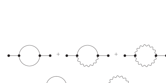
Figure 4: One loop corrections to the scalar power spectrum. Straight lines represent the $\zeta$ propagator while the graviton propagator is wavy.

The various diagrams which contribute to the one loop correction to $\Delta^{2}_{\mathcal{R}}(k)$ are depicted in Figure 4. In each case the leftmost point is fixed at $x^{\mu}=(t,\vec{x})$ and the rightmost point is fixed at ${x^{\prime}}^{\mu}=(t,\vec{0})$. Interior points are integrated. For example, the leftmost diagram on the first line has the general form,

$$\int\!\!d^{D}y\,i\Delta_{\zeta}(x;y)V_{\zeta^{3}}(y)\!\!\int\!\!d^{D}y^{\prime}\,i\Delta_{\zeta}(x^{\prime};y^{\prime})V_{\zeta^{3}}(y^{\prime})\Bigl{[}i\Delta_{\zeta}(y;y^{\prime})\Bigr{]}^{2}\;,$$ (115)

where $V_{\zeta^{3}}(y)$ and $V_{\zeta^{3}}(y^{\prime})$ denote the vertex operators one can read off from the $\zeta^{3}$ interaction. To recover the ordering in (56) the $x^{\mu}$ line must have $-$ polarity and the ${x^{\prime}}^{\mu}$ must be $+$, while the $y^{\mu}$ and ${y^{\prime}}^{\mu}$ vertices would be summed over all $\pm$ variations.

I will return to the possibility that vertex integrations lead to temporal growth but for now let me assume that the two net derivatives in each vertex combine with the associated integral to produce a factor of $c/H^{2}$. Under this assumption one can estimate the strength of any diagram by combining:

• A factor of $\hbar GH^{2}/c^{5}\epsilon$ for each $\zeta$ propagator;

• A factor of $\hbar GH^{2}/c^{5}$ for each $h_{ij}$ propagator; and

• A factor of $c^{5}\epsilon^{N}/\hbar GH^{2}$ for each vertex with either $2N-1$ or $2N$ $\zeta$ fields and any number of $h_{ij}$ fields.

For example, the estimated result for the leftmost diagram on the first line of Figure 4 is,

$$\Bigl{(}\frac{\hbar GH^{2}}{c^{5}\epsilon}\Bigr{)}^{4}\times\Bigl{(}\frac{\hbar GH^{2}}{c^{5}}\Bigr{)}^{0}\times\Bigl{(}\frac{c^{5}\epsilon^{2}}{\hbar GH^{2}}\Bigr{)}^{2}=\Bigl{(}\frac{\hbar GH^{2}}{c^{5}\epsilon}\Bigr{)}^{2}=\Bigl{(}\frac{\hbar GH^{2}}{c^{5}\epsilon}\Bigr{)}\times\Bigl{(}\frac{\hbar GH^{2}\epsilon}{c^{5}}\Bigr{)}\;.$$ (116)

In the final expression of (116) I have extracted the tree order result (71), so one sees that this one loop correction is down by the factor of $\hbar GH^{2}/c^{5}$ (which was inevitable on dimensional grounds) times an extra factor of $\epsilon$. Neither of the two diagrams on the bottom line of Figure 4 has this extra suppression,

$$\Bigl{(}\frac{\hbar GH^{2}}{c^{5}\epsilon}\Bigr{)}^{3}\times\Bigl{(}\frac{\hbar GH^{2}}{c^{5}}\Bigr{)}^{0}\times\Bigl{(}\frac{c^{5}\epsilon^{2}}{\hbar GH^{2}}\Bigr{)}^{1} = \Bigl{(}\frac{\hbar GH^{2}}{c^{5}\epsilon}\Bigr{)}\times\Bigl{(}\frac{\hbar GH^{2}}{c^{5}}\Bigr{)}\;,$$ (117)

$$\Bigl{(}\frac{\hbar GH^{2}}{c^{5}\epsilon}\Bigr{)}^{2}\times\Bigl{(}\frac{\hbar GH^{2}}{c^{5}}\Bigr{)}^{1}\times\Bigl{(}\frac{c^{5}\epsilon}{\hbar GH^{2}}\Bigr{)}^{1} = \Bigl{(}\frac{\hbar GH^{2}}{c^{5}\epsilon}\Bigr{)}\times\Bigl{(}\frac{\hbar GH^{2}}{c^{5}}\Bigr{)}\;.$$ (118)

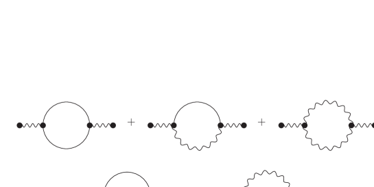
Figure 5: One loop corrections to the tensor power spectrum. Straight lines represent the $\zeta$ propagator while the graviton propagator is wavy.

The one loop corrections to $\Delta^{2}_{h}(k)$ are depicted in Figure 5. The same rules suffice to estimate the strengths of these corrections, although one must recall that the tree order result (71) has no $\epsilon$ enhancement. For example, the leftmost diagram on the first line of Figure 5 contributes,

$$\Bigl{(}\frac{\hbar GH^{2}}{c^{5}\epsilon}\Bigr{)}^{2}\times\Bigl{(}\frac{\hbar GH^{2}}{c^{5}}\Bigr{)}^{2}\times\Bigl{(}\frac{c^{5}\epsilon}{\hbar GH^{2}}\Bigr{)}^{2}=\Bigl{(}\frac{\hbar GH^{2}}{c^{5}}\Bigr{)}\times\Bigl{(}\frac{\hbar GH^{2}}{c^{5}}\Bigr{)}\;.$$ (119)

None of the one loop corrections to $\Delta^{2}_{h}(k)$ is any stronger than (119); the central diagram on the first line is actually suppressed by an additional factor of $\epsilon$. We therefore conclude that one loop corrections to each of the power spectra are generically suppressed from the tree results (71) by a factor of $\hbar GH^{2}/c^{5}\sim 10^{-10}$.

In these estimates it will be noted that I have not specified when the various factors of $H(t)$ and $\epsilon(t)$ are evaluated. Both quantities are thought to be nearly constant during much of primordial inflation — in which case, it does not matter much when they are evaluated. However, it is well to recall that the actual loop corrections are integrals of sometimes differentiated propagators, like expression (115). Weinberg noted the possibility for these integrations to grow with the co-moving time [20]. That this can happen is associated with infrared divergences of the $\zeta$ and $h_{ij}$ propagators which are evident from the small $k$ limiting form (69) of both mode functions for constant $\epsilon$ [114]. This leads to two sources of possible secular growth:

• A coincident propagator — such as the four diagrams on the bottom lines of Figures 4 and 5 — grows like $\hbar GH^{2}/c^{5}\times Ht$ [115, 116, 45]; and

• When the analogous in-out expression would be infrared divergent, a Schwinger-Keldysh integration such as (105) is finite but grows with time [117].

The physical origin of both effects is that even the long wave length parts of the $\zeta$ and $h_{ij}$ effective actions are affected by the on-going process of inflationary particle production.

Weinberg proved an important theorem which limits the growth of loop corrections to the primordial power spectra for the single-scalar model (27) plus an arbitrary number of free scalars which are minimally coupled to gravity [21]. His result is that the largest possible secular enhancement to the depressingly small estimates (118) and (119) consists of powers of the number of inflationary e-foldings. His student Bua Chaicherdsakul extended the result to cover fermions and gauge particles [118]. However, the situation changes radically if one allows matter couplings to the inflaton because the resulting Coleman-Weinberg corrections to its effective potential can induce important changes in the expansion history. For example, if an $m^{2}\varphi^{2}$ inflaton were coupled to a massless fermion the resulting negative energy Coleman-Weinberg correction would cause the universe to end in a Big Rip singularity [119]. Because the gauge (37) forces the inflaton to agree with its classical trajectory, changes in the physical expansion history manifest in secular growth of $\zeta(t,\vec{x})$ correlators. It should also be noted that Weinberg’s theorem is limited to the inflationary power spectra. Explicit computations show that loop corrections to other correlators such as the vacuum polarization [120] and the fermion self-energy [121] can grow like powers of the inflationary scale factor.

3 Nonlinear Extensions

No one disputes Weinberg’s bound, but some cosmologists disagree that there can be any secular corrections. Weinberg gave two examples [20], which other authors confirmed [122]. However, Senatore and Zaldarriaga identified a problem with the use of dimensional regularization in one of these examples, and went on to argue that no secular enhancements are possible under any circumstances [123]. It seems very clear that models can be devised for which quantum corrections to the naive correlators (56-57) grow with time like powers of the number of e-foldings, just as Weinberg stated [70]. Close examination of claims to the contrary [124, 125, 126] reveals that the authors are not actually disputing this, but rather arguing that the naive correlators (56-57) should be replaced with other theoretical quantities which fail to show secular growth. That brings up the fascinating and crucial issue of what operators represent the measured power spectra.

The problem with trying to overcome the loop suppression through secular enhancements is that the growth begins at first horizon crossing and terminates with the end of inflation. But observable modes experienced first horizon crossing at most 50 e-foldings before the end of inflation, which means the enhancement can be at most some small power of 50. The issue which focussed people’s attention on modifying the naive observables was not secular growth but rather the closely associated problem of sensitivity to the infrared cutoff. Ford and Parker showed in 1977 that the propagator of a massless, minimally coupled scalar has an infrared divergence for any constant $\epsilon(t)$ cosmology in the range $0\leq\epsilon\leq\frac{3}{2}$ [114]. In view of relations (67-67) this same problem afflicts both the $\zeta$ and $h_{ij}$ propagators. Like all infrared divergences, this one derives from posing an unphysical question. The problem in this case is arranging large correlations for super-horizon modes which no local observer can control. There are two fixes which have been suggested:

• Either arrange for the initially super-horizon modes to be in some less highly correlated state [127]; or else

• Work on a spatially compact manifold such as $T^{D-1}$ whose coordinate radius is such that there are no initially super-horizon modes [128].

In practice each fix amounts to cutting off the Fourier mode sum at some minimum value $k=L^{-1}$. If infrared divergences could be shown to afflict loop corrections to the power spectra, and if the cutoff $L$ were large enough, then loop corrections might be significant.

I recommend the review article by Seery on infrared loop corrections to inflationary correlators [129]. Important work was done by a number of authors [130, 131, 132, 133, 134, 135, 136, 137, 138, 139, 140, 141, 142, 143]. In 2010 Giddings and Sloth were able to give a convincing argument that graviton loop corrections to $\Delta^{2}_{\mathcal{R}}(k)$ are indeed sensitive to the infrared cutoff $L$ [144, 145], and hence able to make significant corrections. This disturbed people who think about gauge invariance in gravity because the actual infrared divergence — as opposed to the closely associated secular growth factor — is a constant in space and time, and a constant field configuration $h_{ij}(t,\vec{x})$ ought to be gauge equivalent to zero. Even before the work of Giddings and Sloth the possibility of such corrections had prompted Urakawa and Tanaka to argue for modifying the original definition (56) so that the spatial argument of the first field $\zeta(t,\vec{x})$ is replaced by the metric-dependent geodesic $\vec{X}[g](\vec{x})$ which is a constant invariant length $\|\vec{x}\|$ from the other point $\vec{0}$ in the direction $\vec{x}$ [146, 147],

$$\Delta^{2}_{\mathcal{R}}(k,t)\longrightarrow\frac{k^{3}}{2\pi^{2}}\int\!\!d^{3}x\,e^{-i\vec{k}\cdot\vec{x}}\Bigl{\langle}\Omega\Bigl{|}\zeta\Bigl{(}t,\vec{X}[g](\vec{x}\Bigr{)}\zeta(t,\vec{0})\Bigr{|}\Omega\Bigr{\rangle}\;.$$ (120)

After the paper by Giddings and Sloth it was quickly established that these sorts of partially invariant observables are free of the infrared divergence [148, 149, 150, 151, 152, 153, 154]. In subsequent work Giddings and Sloth have sought to identify invariant observables which still show the enhancement [155, 156]. Tanaka and Urakawa have also continued their work on the problem, [157, 158, 159, 160]

The discussion of infrared effects attracted me because I had for years been working on these in de Sitter background. I was also fascinated by the struggle to identify physical observables in quantum gravity because my long-neglected doctoral thesis dealt with that very subject [18]. In fact had I considered corrections involving precisely the same sort of geodesics as in (120)! One thing I discovered is that they introduce new ultraviolet divergences associated with integrating graviton fields over the 1-dimensional background geodesic [18]. These new divergences change the power spectrum into the expectation value of a nonlocal composite operator which no one currently understands how to renormalize [22]. Shun-Pei Miao and I also demonstrated that (120) disturbs the careful pattern of $\epsilon$-suppression which we saw section 2; one loop corrections to (120) go like the tree order result (71) times $\hbar GH^{2}/c^{5}\epsilon$ [22]. For the very same reason, non-Gaussianity would also be unsuppressed [22]. So changing what theoretical quantity we identify with the scalar power spectrum from (56) to (120) in order to avoid sensitivity on the infrared cutoff would come at the high price of introducing uncontrollable ultraviolet divergences and observable non-Gaussianity. It seems a bad bargain, and I mean no disrespect to colleagues who are struggling to puzzle out the truth, as am I, when I say we must do better.

It seems clear to me that we need new ideas. One radical and thought-provoking proposal is the suggestion by Miao and Park to abandon correlators altogether and instead quantum-correct the mode function relations (64-65) [23]. Among other things, this would avoid the new ultraviolet divergence which Fröb, Roura and Verdaguer have found in one loop corrections to the tensor power spectrum because the two times coincide [161].

It also seems to me that too few physicists appreciate the wondrous opportunity which has befallen us to shape a new discipline by defining its observables. The debate on this vital subject is sometimes confused, and too often degenerates into shouting matches. In an effort to clarify matters Shun-Pei Miao and I laid out ten principles which are worth repeating here [22]:

1. IR divergence differs from IR growth;

2. The leading IR logs might be gauge independent;

3. Not all gauge dependent quantities are unphysical;

4. Not all gauge invariant quantities are physical;

5. Nonlocal “observables” can null real effects;

6. Renormalization is crucial and unresolved;

7. Extensions involving $\zeta$ must be $\epsilon$-suppressed;

8. It is important to acknowledge approximations;

9. Sub-horizon modes cannot have large IR logs; and

10. Spatially constant quantities are observable.

4 The Promise of 21cm Radiation

Particle physicists are familiar with the saying, “yesterday’s discovery is tomorrow’s background.” Cosmologists are today witnessing the final stages of this process in the context of observations of the cosmic microwave background, as interlocking developments in technology and understanding of astrophysical processes have permitted fundamental theory to be probed more and more deeply. A brief survey of the history is instructive:

• 1964 — discovery of the monopole, for which Penzias and Wilson received the 1978 Nobel Prize;

• 1970’s — discovery of the dipole, which gives the Earth’s motion relative to the CMB;

• 1992 — discovery of lowest higher multipoles in the temperature-temperature correlator by COBE, for which Mather and Smoot received the 2006 Nobel Prize;

• 1999 — detection of the first Doppler peak by BOOMERanG and MAXIMA, supporting inflation and not cosmic strings as the primary source of structure formation;

• early 2000’s — detection of $E$-mode polarization by DASI and CBI, and demonstration by WMAP of the $T$-$E$ anti-correlation predicted by inflation;

• 2003-2010 — full sky maps of temperature and $E$-mode correlators by WMAP, and their use for precision determinations of cosmological parameters;

• 2013 — full sky map of Planck resolves seven Doppler peaks and give tighter bounds on $\Lambda$CDM parameters;

• 2013 — First detection of $B$-mode polarization from gravitational lensing by the South Pole Telescope;

• 2014 — Detection of primordial $B$-mode polarization claimed by BICEP2, confirming another key prediction of primordial inflation, fixing the inflationary energy scale to be $\sim 2\times 10^{16}~{}{\rm GeV}$, and incidentally establishing the existence and quantization of gravitons; and

• 2014 — Resolution of six acoustic peaks of $E$-mode polarization by the Atacama Cosmology Telescope Polarimeter, which provides an independent determination of $\Lambda$CDM parameters.

The first steps are even now being taken in what could be an equally fruitful evolution, whose full realization will consume decades as it yields a steady series of discoveries. I refer to the project of surveying large volumes of the Universe using the 21 cm line [162]. The discovery potential is obvious from the comparison between an x-ray and a CT-scan: all that has been learned from the cosmic microwave background derives from the surface of last scattering, whereas 21 cm radiation allows us to make a tomograph of the universe.

Current and planned projects probe two regimes of cosmic redshift:

• $0\mathrel{\raise 1.29167pt\hbox{$<$\kern-7.5pt\lower 4.30554pt\hbox{$\sim$}}}z\mathrel{\raise 1.29167pt\hbox{$<$\kern-7.5pt\lower 4.30554pt\hbox{$\sim$}}}4$ — in which the radiation from unresolved galaxies is observed to probe baryon acoustic oscillations [163, 164, 165, 166, 167, 168].

• $6\mathrel{\raise 1.29167pt\hbox{$<$\kern-7.5pt\lower 4.30554pt\hbox{$\sim$}}}z\mathrel{\raise 1.29167pt\hbox{$<$\kern-7.5pt\lower 4.30554pt\hbox{$\sim$}}}10$ — in which intergalactic Hydrogen is observed to probe the epoch of reionization [169, 170, 171, 172, 173].

The first of these provides important information for understanding the mysterious physics which is causing the current universe to accelerate, the discovery of which earned Perlmutter, Schmidt and Riess the 2011 Nobel Prize. The second is crucial to understanding the first generation of stars, and will eventually be an important foreground in future observations.

As technology and engineering improve, and as astrophysical effects are better understood, it is possible to foresee a time (decades from now) when redshifts as high as $z\sim 50$ are observed to measure the matter power spectrum with staggering accuracy. There is enough potentially recoverable data in the 21 cm radiation to resolve one loop corrections [174]. Current measurements of $\Delta^{2}_{\mathcal{R}}(k)$ do not test fundamental theory because we lack a compelling mechanism for driving primordial inflation, but that is bound to change over the decades required for the full maturity of 21 cm cosmology. And when we do understand the driving mechanism, it will be possible to untangle the one loop correction from the tree order effect, which will test quantum gravity. This could be for quantum gravity what the measurement of $g-2$ was for quantum electrodynamics. The data is there, and people will be working for decades to harvest it.

5 Other Quantum Gravitational Effects

As I have explained, the driving force for quantum gravitational effects during inflation is the production of nearly massless, minimally coupled scalars (if there are any) and gravitons. The presence of these particles is quantified by the scalar and tensor power spectra. Because Einstein + anything is an interacting quantum field theory, the newly created particles must interact, at some level, both with themselves and with other particles. This section describes how to study those interactions. I first list the various linearized effective field equations, then I describe the propagators and how to represent the tensor structure of the associated one-particle-irreducible (1PI) 2-point functions. The section closes with a review of results and open problems. However, the issue of back-reaction is so convulted and contentious that it merits its own subsection.

1 Linearized Effective Field Equations

We want to study how the propagation of a single particle is affected by the vast sea of infrared gravitons and scalars produced by inflation. That can be done by computing the 1PI 2-point function of the particle in question and then using it to quantum-correct the linearized effective field equation. Recall from (10) that quantum gravitational loop corrections from inflationary particle production are suppressed by $\hbar GH_{i}^{2}/c^{5}\sim 10^{-10}$. Because this number is so small it is seldom necessary include nonlinear effects or to go beyond one loop order. The usual unit conventions of relativistic quantum field theory apply in which time is measured so that $c=1$, and mass is measured so that $\hbar=1$. The loop-counting parameter of quantum gravity is $\kappa^{2}\equiv 16\pi G(\times\hbar/c^{3})\approx 1.3\times 10^{-69}~{}{\rm m}^{2}$.

Because $\epsilon_{i}\approx 0.013$ is so small, most work is done on de Sitter background, for which $\epsilon(t)=0$ and $H(t)$ is a constant. Computations are done on a portion of the full de Sitter manifold which is termed “the cosmological patch” in the recent literature, and sometimes “open conformal coordinates” in the older literature,

$$ds^{2}=a^{2}(\eta)\Bigl{[}-d\eta^{2}+d\vec{x}\!\cdot\!d\vec{x}\Bigr{]}\qquad,\qquad a(\eta)\equiv-\frac{1}{H\eta}=e^{Ht}\;.$$ (121)

The $D-1$ spatial coordinates exist in the same range $-\infty<x^{i}<+\infty$ as Minkowski space, but the conformal time $\eta$ is limited to the range $-\infty<\eta\leq 0$. The de Sitter metric is $g_{\mu\nu}=a^{2}\eta_{\mu\nu}$, where $\eta_{\mu\nu}$ is the Minkowski metric. In contrast to section 4, metric fluctuations are characterized by the conformally rescaled and canonically normalized graviton field $h_{\mu\nu}$,

$$g^{\rm full}_{\mu\nu}(x)\equiv a^{2}\Bigl{[}\eta_{\mu\nu}+\kappa h_{\mu\nu}(x)\Bigr{]}\;.$$ (122)

Graviton indices are raised and lowered with the Minkowski metric, $h^{\mu}_{~{}\nu}\equiv\eta^{\mu\rho}h_{\rho\nu}$, $h^{\mu\nu}\equiv\eta^{\mu\rho}\eta^{\nu\sigma}h_{\rho\sigma}$, $h\equiv\eta^{\mu\nu}h_{\mu\nu}$. Fermion fields are also conformally rescaled,

$$\psi^{\rm full}_{i}(x)\equiv a^{\frac{D-1}{2}}\times\psi_{i}(x)\;.$$ (123)

The various 1PI 2-point functions are evaluated using dimensional regularization, then fully renormalized with the appropriate counterterms in the sense of Bogoliubov, Parasiuk [175], Hepp [176] and Zimmermann [177, 178] (BPHZ). After this the unregulated limit of $D=4$ is taken. As explained in section 1, quantum corrections to the in-out effective field equations at spacetime point $x^{\mu}$ are dominated by contributions from points ${x^{\prime}}^{\mu}$ in the infinite future when the 3-volume has been expanded to infinity. Quantum corrections to the in-out matrix elements of field operators are also generally complex, even for real fields. These results are correct for in-out scattering theory, but they have no physical relevance for cosmology where the appropriate question is what happens to the expectation value of the field operator in the presence of a prepared state which is released at some finite time. One solves that sort of problem using the Schwinger-Keldysh formalism [104, 105, 106, 107]. In this technique each of the 1PI $N$-point functions of the in-out formalism gives rise to $2^{N}$ Schwinger-Keldysh $N$-point functions. It is the sum of the $++$ and $+-$ 1PI 2-point functions which appears in the linearized Schwinger-Keldysh effective field equation. This combination is both real and causal.

The 1PI 2-point function for a scalar is known as its “self-mass-squared”, $-iM^{2}(x;x^{\prime})$. The quantum-corrected, linearized field equation for a minimally coupled scalar with mass $m$ is,

$$a^{2}\Bigl{(}-\partial^{2}_{0}-2Ha\partial_{0}+\nabla^{2}\Bigr{)}\varphi(x)-m^{2}a^{4}\varphi(x)-\int\!\!d^{4}x^{\prime}M^{2}(x;x^{\prime})\varphi(x^{\prime})=0\;.$$ (124)

The (conformally rescaled) fermion’s 1PI 2-point function is called its “self-energy”, $-i[\mbox{}_{i}\Sigma_{j}](x;x^{\prime})$. If $\gamma^{\mu}_{ij}$ stands for the usual gamma matrices then the quantum-corrected, linearized field equation for a fermion with mass $m$ is,

$$i\gamma^{\mu}_{ij}\partial_{\mu}\psi_{j}(x)-ma\psi_{i}(x)-\int\!\!d^{4}x^{\prime}\Bigl{[}\mbox{}_{i}\Sigma_{j}\Bigr{]}(x;x^{\prime})\psi_{j}(x^{\prime})=0\;.$$ (125)

The 1PI 2-point function for a photon has the evocative name “vacuum polarization”, $+i[\mbox{}^{\mu}\Pi^{\nu}](x;x^{\prime})$. If $F^{\nu\mu}\equiv\eta^{\nu\rho}\eta^{\mu\sigma}(\partial_{\rho}A_{\sigma}-\partial_{\sigma}A_{\rho})$ is the usual field strength tensor then the quantum-corrected Maxwell equation can be written,

$$\partial_{\nu}F^{\nu\mu}(x)+\int\!\!d^{4}x^{\prime}\Bigl{[}\mbox{}^{\mu}\Pi^{\nu}\Bigr{]}(x;x^{\prime})A_{\nu}(x^{\prime})=J^{\nu}(x)\;,$$ (126)

where $J^{\mu}(x)$ is the current density. Finally, the 1PI 2-point function for a (conformally rescaled and canonically normalized) graviton is termed the “graviton self-energy”, $-i[\mbox{}^{\mu\nu}\Sigma^{\rho\sigma}](x;x^{\prime})$. It is used to quantum correct the linearized Einstein equation as,

$$\partial_{\alpha}\Bigl{[}a^{2}\mathcal{L}^{\mu\nu\alpha\beta\rho\sigma}\partial_{\beta}h_{\rho\sigma}(x)\Bigr{]}-\int\!\!d^{4}x^{\prime}\Bigl{[}\mbox{}^{\mu\nu}\Sigma^{\rho\sigma}\Bigr{]}(x;x^{\prime})h_{\rho\sigma}(x^{\prime})=-\frac{\kappa a^{2}}{2}\eta^{\mu\rho}\eta^{\nu\sigma}T_{\rho\sigma}(x)\;,$$ (127)

where $T_{\rho\sigma}$ is the linearized stress tensor and I define,

$$\mathcal{L}^{\mu\nu\rho\sigma\alpha\beta}\equiv\frac{1}{2}\eta^{\alpha\beta}\Bigl{[}\eta^{\mu(\rho}\eta^{\sigma)\nu}\!-\!\eta^{\mu\nu}\eta^{\rho\sigma}\Bigr{]}$$ (128)

$$\hskip 99.58464pt+\frac{1}{2}\eta^{\mu\nu}\eta^{\rho(\alpha}\eta^{\beta)\sigma}+\frac{1}{2}\eta^{\rho\sigma}\eta^{\mu(\alpha}\eta^{\beta)\nu}-\eta^{\alpha)(\rho}\eta^{\sigma)(\mu}\eta^{\nu)(\beta}\;.\qquad$$

The scalar equation (124) and its spinor counterpart (125) of course describe the propagation of scalars and spinors, respectively. The vector and tensor equations (126-127) can be similarly used to study the propagation of dynamical photons and gravitons, but they also describe modifications of the electrodynamic and gravitational forces. Dynamical quanta show no modification in flat space quantum field theory (enforcing that is what typically fixes the field strength renormalization) so it is at least possible that nothing happens as well during inflation. However, the force laws are guaranteed to show an effect during inflation because they do so in flat space background [179, 180, 181].

2 Propagators and Tensor 1PI Functions

The symmetries of the general cosmological geometry (1) are homogeneity and isotropy. However, the de Sitter limit of $\epsilon(t)=0$ results in the appearance of two additional symmetries. Although it obvious to cosmologists that these extra symmetries can be at best approximate for inflationary cosmology, they have exerted a powerful influence on mathematical physicists owing to the expectation that the full de Sitter group should play the same role in organizing and simplifying quantum field theory on de Sitter that Poincaré invariance has played for flat space. That expectation has remained unfulfilled owing to the time dependence intrinsic to inflationary particle production.

In our $D$-dimensional conformal coordinate system (121) the $\frac{1}{2}D(D+1)$ de Sitter transformations can be decomposed as follows:

• $(D-1)$ spatial tranlations,

  $$\eta^{\prime}=\eta\;,~{}~{}x^{\prime i}=x^{i}+\epsilon^{i}\;.$$ (129)

• $\frac{1}{2}(D-1)(D-2)$ spatial rotations,

  $$\eta^{\prime}=\eta\;,~{}~{}x^{\prime i}=R^{ij}x^{j}\;.$$ (130)

• One dilatation,

  $$\eta^{\prime}=k\eta\;,~{}~{}x^{\prime i}=kx^{j}\;.$$ (131)

• $(D-1)$ spatial special conformal transformations,

  $$\eta^{\prime}=\frac{\eta}{1-2\vec{\theta}\cdot\vec{x}+\parallel\!\vec{\theta}\!\parallel^{2}x\cdot x}\;,~{}~{}x^{\prime}=\frac{x^{i}-\theta^{i}x\cdot x}{1-2\vec{\theta}\cdot\vec{x}+\parallel\!\vec{\theta}\!\parallel^{2}x\cdot x}\;.$$ (132)

Homogeneity is (129) and isotropy is (130). The two additional symmetries which appear in the de Sitter limit of $\epsilon(t)=0$ are (131-132).

Although infrared divergences induce de Sitter breaking, they do so in a limited way that leaves the largest part of the result de Sitter invariant. For dimensional regularization computations it is best to express this de Sitter invariant part in terms of the length function $y(x;z)$,

$$y(x;x^{\prime})\equiv aa^{\prime}H^{2}\Bigl{[}\Bigl{\|}\vec{x}\!-\!\vec{x}^{\prime}\Bigr{\|}^{2}-\Bigl{(}|\eta\!-\!\eta^{\prime}|\!-\!i\varepsilon\Bigr{)}^{2}\Bigr{]}\;.$$ (133)

Except for the factor of $i\varepsilon$ (whose purpose is to enforce Feynman boundary conditions) the function $y(x;x)$ is related to the invariant length $\ell(x;x^{\prime})$ from $x^{\mu}$ to ${x^{\prime}}^{\mu}$,

$$y(x;x^{\prime})=4\sin^{2}\Bigl{(}\frac{1}{2}H\ell(x;x^{\prime})\Bigr{)}\;.$$ (134)

The four Schwinger-Keldysh polarity variations (101-104) never affect the de Sitter breaking terms. They can all be obtained by making simple changes of the $i\varepsilon$ term in (133),

$$y_{\scriptscriptstyle++}(x;x^{\prime}) = aa^{\prime}H^{2}\Bigl{[}\Bigl{\|}\vec{x}\!-\!\vec{x}^{\prime}\Bigr{\|}^{2}-\Bigl{(}|\eta\!-\!\eta^{\prime}|\!-\!i\varepsilon\Bigr{)}^{2}\Bigr{]}\;,$$ (135)

$$y_{\scriptscriptstyle-+}(x;x^{\prime}) = aa^{\prime}H^{2}\Bigl{[}\Bigl{\|}\vec{x}\!-\!\vec{x}^{\prime}\Bigr{\|}^{2}-\Bigl{(}\eta\!-\!\eta^{\prime}\!-\!i\varepsilon\Bigr{)}^{2}\Bigr{]}\;,$$ (136)

$$y_{\scriptscriptstyle+-}(x;x^{\prime}) = aa^{\prime}H^{2}\Bigl{[}\Bigl{\|}\vec{x}\!-\!\vec{x}^{\prime}\Bigr{\|}^{2}-\Bigl{(}\eta\!-\!\eta^{\prime}\!+\!i\varepsilon\Bigr{)}^{2}\Bigr{]}\;,$$ (137)

$$y_{\scriptscriptstyle--}(x;x^{\prime}) = aa^{\prime}H^{2}\Bigl{[}\Bigl{\|}\vec{x}\!-\!\vec{x}^{\prime}\Bigr{\|}^{2}-\Bigl{(}|\eta\!-\!\eta^{\prime}|\!+\!i\varepsilon\Bigr{)}^{2}\Bigr{]}\;.$$ (138)

The best way of expressing higher spin propagators on de Sitter, as on flat space, is by acting differential operators on scalar propagators. I work with a general scalar propagator $i\Delta_{b}(x;x^{\prime})$ which obeys the equation,

$$\Bigl{[}\kern 1.0pt\vbox{\hrule height=1.2pt\hbox{\vrule width=1.2pt\hskip 3.0pt\vbox{\vskip 6.0pt}\hskip 3.0pt\vrule width=0.6pt}\hrule height=0.6pt}\kern 1.0pt+(b^{2}\!-\!b_{A}^{2})H^{2}\Bigr{]}i\Delta_{b}(x;x^{\prime})=\frac{i\delta^{D}(x\!-\!x^{\prime})}{\sqrt{-g}}\;.$$ (139)

Here and henceforth the index $b_{A}$ is $b_{A}\equiv\frac{D-1}{2}$ and        stands for the covariant scalar d’Alembertian,

$$\kern 1.0pt\vbox{\hrule height=1.2pt\hbox{\vrule width=1.2pt\hskip 3.0pt\vbox{\vskip 6.0pt}\hskip 3.0pt\vrule width=0.6pt}\hrule height=0.6pt}\kern 1.0pt\equiv\frac{1}{\sqrt{-g}}\,\partial_{\mu}\Bigl{(}\sqrt{-g}\,g^{\mu\nu}\partial_{\nu}\Bigr{)}=\frac{1}{a^{2}}\Bigl{(}-\partial_{0}^{2}-(D\!-\!2)Ha\partial_{0}+\nabla^{2}\Bigr{)}\;.$$ (140)

For the case of $b<b_{A}$ the propagator has a positive mass-squared $m^{2}=(b_{A}^{2}-b^{2})H^{2}$ and its propagator is a de Sitter invariant Hypergeometric function of $y(x;x^{\prime})$. Its expansion for $b=\nu$ is,

$$i\Delta^{\rm dS}_{\nu}(x;x^{\prime})=\frac{H^{D-2}}{(4\pi)^{\frac{D}{2}}}\Biggl{\{}\Gamma\Bigl{(}\frac{D}{2}\!-\!1\Bigr{)}\Bigl{(}\frac{4}{y}\Bigr{)}^{\frac{D}{2}-1}-\frac{\Gamma(\frac{D}{2})\Gamma(1\!-\!\frac{D}{2})}{\Gamma(\frac{1}{2}\!+\!\nu)\Gamma(\frac{1}{2}\!-\!\nu)}\sum_{n=0}^{\infty}$$ (141)

$$\times\Biggl{[}\frac{\Gamma(\frac{3}{2}\!+\!\nu\!+\!n)\Gamma(\frac{3}{2}\!-\!\nu\!+\!n)}{\Gamma(3\!-\!\frac{D}{2}\!+\!n)\,(n\!+\!1)!}\Bigl{(}\frac{y}{4}\Bigr{)}^{n-\frac{D}{2}+2}\!\!\!-\!\frac{\Gamma(b_{A}\!+\!\nu\!+\!n)\Gamma(b_{A}\!-\!\nu\!+\!n)}{\Gamma(\frac{D}{2}\!+\!n)\,n!}\Bigl{(}\frac{y}{4}\Bigr{)}^{n}\Biggr{]}\!\Biggr{\}}.\qquad$$

When $b\geq b_{A}$ the naive mode sum is infrared divergent for the same reason as the problem discovered by Ford and Parker [114] which I described in section 3. One sometimes encounters contrary statements in the mathematical physics literature [182], but close examination reveals that the authors admit they are constructing a formal solution to the propagator equation which is not a true propagator by the illegitimate technique of adding negative norm states to the theory [183]. The proper technique [127, 128] of cutting off the mode sum amounts to adding to (141) a de Sitter breaking, infrared correction [184, 185],

$$\Delta^{\rm IR}_{\nu}(x;x^{\prime})=\frac{H^{D-2}}{(4\pi)^{\frac{D}{2}}}\frac{\Gamma(\nu)\Gamma(2\nu)}{\Gamma(b_{A})\Gamma(\nu\!+\!\frac{1}{2})}\times\theta(\nu\!-\!b_{A})$$ (142)

$$\hskip 19.91684pt\times\sum_{N=0}^{[\nu-b_{A}]}\frac{(aa^{\prime})^{\nu-b_{A}-N}}{\nu\!-\!b_{A}\!-\!N}\sum_{n=0}^{N}\Bigl{(}\frac{a}{a^{\prime}}\!+\!\frac{a^{\prime}}{a}\Bigr{)}^{n}\sum_{m=0}^{[\frac{N-n}{2}]}C_{Nnm}(y\!-\!2)^{N-n-2m}\;,\qquad$$

where the coefficients $C_{Nnm}$ are,

$$C_{Nnm}=\frac{(-\frac{1}{4})^{N}}{m!n!(N\!-\!n\!-\!2m)!}\times\frac{\Gamma(b_{A}\!+\!N\!+\!n\!-\!\nu)}{\Gamma(b_{A}\!+\!N\!-\!\nu)}$$ (143)

$$\hskip 56.9055pt\times\frac{\Gamma(b_{A})}{\Gamma(b_{A}\!+\!N\!-\!2m)}\times\frac{\Gamma(1\!-\!\nu)}{\Gamma(1\!-\!\nu\!+\!n\!+\!2m)}\times\frac{\Gamma(1\!-\!\nu)}{\Gamma(1\!-\!\nu\!+\!m)}\;.\qquad$$

The full propagator is therefore,

$$i\Delta_{b}(x;x^{\prime})=\lim_{\nu\rightarrow b}\Bigl{[}i\Delta^{\rm dS}_{\nu}(x;x^{\prime})+\Delta^{\rm IR}_{\nu}(x;x^{\prime})\Bigr{]}\;.$$ (144)

It is often useful to discuss integrated propagators which obey,

$$\Bigl{[}\kern 1.0pt\vbox{\hrule height=1.2pt\hbox{\vrule width=1.2pt\hskip 3.0pt\vbox{\vskip 6.0pt}\hskip 3.0pt\vrule width=0.6pt}\hrule height=0.6pt}\kern 1.0pt+(b^{2}\!-\!b_{A}^{2})H^{2}\Bigr{]}i\Delta_{bc}(x;z)=i\Delta_{c}(x;z)\;.$$ (145)

The solution is easily seen to be [185, 186],

$$i\Delta_{bc}(x;z)=\frac{1}{(b^{2}\!-\!c^{2})H^{2}}\Bigl{[}i\Delta_{c}(x;z)\!-\!i\Delta_{b}(x;z)\Bigr{]}=i\Delta_{cb}(x;z)\;.$$ (146)

I also employ a doubly integrated propagator which obeys,

$$\Bigl{[}\kern 1.0pt\vbox{\hrule height=1.2pt\hbox{\vrule width=1.2pt\hskip 3.0pt\vbox{\vskip 6.0pt}\hskip 3.0pt\vrule width=0.6pt}\hrule height=0.6pt}\kern 1.0pt+(b^{2}\!-\!b_{A}^{2})H^{2}\Bigr{]}i\Delta_{bcd}(x;z)=i\Delta_{cd}(x;z)\;.$$ (147)

The solution can be written in a form which is manifestly symmetric under any interchange of the three indices $a$, $b$ and $c$,

$$i\Delta_{bcd}(x;z) \!\!=\!\! \frac{i\Delta_{bd}(x;z)\!-\!i\Delta_{bc}(x;z)}{(c^{2}\!-\!d^{2})H^{2}}\;,\qquad$$ (148)

$$\!\!=\!\! \frac{(d^{2}\!-\!c^{2})i\Delta_{b}(x;z)\!+\!(b^{2}\!-\!d^{2})i\Delta_{c}(x;z)\!+\!(c^{2}\!-\!b^{2})i\Delta_{d}(x;z)}{(b^{2}\!-\!c^{2})(c^{2}\!-\!d^{2})(d^{2}\!-\!b^{2})H^{4}}\;.\qquad$$ (149)

The propagator for a (conformally rescaled) fermion of mass $m$ was constructed by Candelas and Raine [187] in terms of the scalar propagator (141) with $\nu=-\frac{1}{2}+i\frac{m}{H}$,

$$i\Bigl{[}\mbox{}_{i}S_{j}\Bigr{]}(x;x^{\prime})=\Bigl{[}i\gamma^{\mu}\partial_{\mu}+am\Bigr{]}(aa^{\prime})^{\frac{D}{2}-1}$$ (150)

$$\hskip 99.58464pt\times\Biggl{\{}\Bigl{(}\frac{I\!-\!\gamma^{0}}{2}\Bigr{)}i\Delta^{\rm dS}_{\nu}(x;x^{\prime})+\Bigl{(}\frac{I\!+\!\gamma^{0}}{2}\Bigr{)}i\Delta^{\rm dS}_{\nu^{*}}(x;x^{\prime})\Biggr{\}}.\qquad$$

Except for the conformal rescaling, expression (150) is de Sitter invariant as long as the mass is real. Tachyonic fermions with $m^{2}\leq-DH^{2}$ break de Sitter invariance the same way that tachyonic scalars do.

Vector and tensor fields raise the issue of gauge fixing. Normally we would accomplish this by adding to the action gauge fixing terms which respect the coordinate isometries of the background, however, there is an obstacle to doing this on any background such as de Sitter which possesses a linearization instability [186]. This leaves two alternatives:

• One either add a de Sitter breaking gauge fixing term which cannot be extended to the full de Sitter manifold; or

• One can impose some gauge condition on the field operators.

After some discussion of the problem I will give results for both alternatives.

The obstacle to adding invariant gauge fixing terms came as a surprise because one can actually derive them in flat space quantum field theory by starting from an exact gauge and making functional changes of variables [188]. In 2009 Miao, Tsamis and I identified precisely where this procedure breaks down when a linearization instability is present [186] but one can see the physics problem quite simply by considering flat space electrodynamics on the manifold $T^{3}\times R$. Because the spatial sections are compact, both sides of the spatially averaged, $\mu=0$ Maxwell equation must vanish separately,

$$\partial_{\nu}F^{\nu\mu}=J^{\mu}\qquad\Longrightarrow\qquad\int_{T^{3}}\!\!d^{3}x\,\partial_{i}F^{i0}(t,\vec{x})=\int_{T^{3}}\!\!d^{3}x\,J^{0}(t,\vec{x})=0\;.$$ (151)

This zero charge constraint follows from the invariant field equations so it must be true in any valid gauge. However, adding a Poincaré invariant gauge fixing term result in a very different theory. The field equations of Feynman gauge are,

$$\Bigl{[}-\partial_{t}^{2}+\nabla^{2}\Bigr{]}A^{\mu}(t,\vec{x})=J^{\mu}(t,\vec{x})\;.$$ (152)

These equations can be solved for any total charge so there cannot be any question that the theory has been changed.

The use of covariant gauge fixing terms is so ingrained that some people’s first reaction to the obstacle on de Sitter is, “let’s just go ahead and do it anyway!” As it happens, Emre Kahya and I had stumbled upon what happens if that is done in 2005. We used two different gauges to compute and fully renormalize the one loop self-mass-squared $-iM^{2}(x;x^{\prime})$ for a charged, massless, minimally coupled scalar on de Sitter [189, 190]. There was no problem with a de Sitter-breaking gauge fixing term [191] — nor is there any problem [192] when Lorentz gauge is enforced as a strong operator condition [193] — but we found on-shell singularities when using the de Sitter-Feynman gauge propagator [194]. The origin of these singularities seems to be that integrating the self-mass-squared against the scalar wave function measures the $A_{0}J^{0}$ interaction of the particle with its own field, and one can see from equation (152) that the solution for $A_{0}(t,\vec{x})$ must grow like $Qt^{2}/2$ in Feynman gauge.

My favorite de Sitter-breaking gauge fixing term for electromagnetism is [191],

$$\mathcal{L}_{GF}=-\frac{1}{2}a^{D-4}\Bigl{(}\eta^{\mu\nu}A_{\mu,\nu}-(D\!-\!4)HaA_{0}\Bigr{)}^{2}\;.$$ (153)

Because space and time components are treated differently it is useful to have an expression for the purely spatial part of the Minkowski metric,

$$\overline{\eta}_{\mu\nu}\equiv\eta_{\mu\nu}+\delta^{0}_{\mu}\delta^{0}_{\nu}\;.$$ (154)

In this gauge the photon propagator takes the form of a sum of constant tensor factors times scalar propagators,

$$i\Bigl{[}{}_{\mu}\Delta_{\nu}\Bigr{]}(x;x^{\prime})=\overline{\eta}_{\mu\nu}\,aa^{\prime}i\Delta_{B}(x;x^{\prime})-\delta^{0}_{\mu}\delta^{0}_{\nu}\,aa^{\prime}i\Delta_{C}(x;x^{\prime})\;.$$ (155)

The B-type and $C$-type propagators are special cases of (141) with $\nu=(D-3)/2$ and $\nu=(D-5)/2$, respectively,

$$i\Delta_{B}(x;x^{\prime})=\frac{H^{D-2}}{(4\pi)^{\frac{D}{2}}}\Biggl{\{}\Gamma\Bigl{(}\frac{D}{2}\!-\!1\Bigr{)}\Bigl{(}\frac{4}{y}\Bigr{)}^{\frac{D}{2}-1}$$ (156)

$$\hskip 85.35826pt+\sum_{n=0}^{\infty}\Biggl{[}\frac{\Gamma(n\!+\!\frac{D}{2})}{\Gamma(n\!+\!2)}\Bigl{(}\frac{y}{4}\Bigr{)}^{n+2-\frac{D}{2}}-\frac{\Gamma(n\!+\!D\!-\!2)}{\Gamma(n\!+\!\frac{D}{2})}\Bigl{(}\frac{y}{4}\Bigr{)}^{n}\Biggr{]}\Biggr{\}},\qquad$$

$$i\Delta_{C}(x;x^{\prime})=\frac{H^{D-2}}{(4\pi)^{\frac{D}{2}}}\Biggl{\{}\Gamma\Bigl{(}\frac{D}{2}\!-\!1\Bigr{)}\Bigl{(}\frac{4}{y}\Bigr{)}^{\frac{D}{2}-1}$$ (157)

$$\hskip 8.5359pt-\sum_{n=0}^{\infty}\Biggl{[}\frac{(n\!-\!\frac{D}{2}\!+\!3)\Gamma(n\!+\!\frac{D}{2}\!-\!1)}{\Gamma(n\!+\!2)}\Bigl{(}\frac{y}{4}\Bigr{)}^{n+2-\frac{D}{2}}\!\!\!-\frac{(n\!+\!1)\Gamma(n\!+\!D\!-\!3)}{\Gamma(n\!+\!\frac{D}{2})}\Bigl{(}\frac{y}{4}\Bigr{)}^{n}\Biggr{]}\Biggr{\}}.\qquad$$

Note that the infinite sums in (156) and (157) vanish for $D=4$, which means they only need to be included when multiplied by a divergence, and even then only the lowest terms of the sums are required. In fact the $B$-type and $C$ type propagators agree in $D=4$, and the photon propagator in this gauge is the same for $D=4$ as it is in flat space! Despite the noncovariant gauge, this propagator shows no physical breaking of de Sitter invariance.

My favorite de Sitter breaking gauge fixing term is [195, 191],

$$\mathcal{L}_{GF}=-\frac{1}{2}a^{D-2}\eta^{\mu\nu}F_{\mu}F_{\nu}\;,\;F_{\mu}\equiv\eta^{\rho\sigma}\Bigl{(}\psi_{\mu\rho,\sigma}-\frac{1}{2}\psi_{\rho\sigma,\mu}+(D\!-\!2)Ha\psi_{\mu\rho}\delta^{0}_{\sigma}\Bigr{)}.$$ (158)

Note that it breaks (132) but preserves (129-131), just like its electromagnetic cousin (153). In this gauge the graviton propagator takes the form of a sum of three constant index factors times a scalar propagator,

$$i\Bigl{[}{}_{\mu\nu}\Delta_{\rho\sigma}\Bigr{]}(x;x^{\prime})=\sum_{I=A,B,C}\Bigl{[}{}_{\mu\nu}T^{I}_{\rho\sigma}\Bigr{]}i\Delta_{I}(x;x^{\prime})\;.$$ (159)

The constant index factors are,

$$\Bigl{[}{}_{\mu\nu}T^{A}_{\rho\sigma}\Bigr{]} = 2\,\overline{\eta}_{\mu(\rho}\overline{\eta}_{\sigma)\nu}-\frac{2}{D\!-\!3}\overline{\eta}_{\mu\nu}\overline{\eta}_{\rho\sigma}\;,$$ (160)

$$\Bigl{[}{}_{\mu\nu}T^{B}_{\rho\sigma}\Bigr{]} = -4\delta^{0}_{(\mu}\overline{\eta}_{\nu)(\rho}\delta^{0}_{\sigma)}\;,$$ (161)

$$\Bigl{[}{}_{\mu\nu}T^{C}_{\rho\sigma}\Bigr{]} = \frac{2}{(D\!-\!2)(D\!-\!3)}\Bigl{[}(D\!-\!3)\delta^{0}_{\mu}\delta^{0}_{\nu}+\overline{\eta}_{\mu\nu}\Bigr{]}\Bigl{[}(D\!-\!3)\delta^{0}_{\rho}\delta^{0}_{\sigma}+\overline{\eta}_{\rho\sigma}\Bigr{]}\;.$$ (162)

The de Sitter invariant $B$-type and $C$-type propagators appear as well in the photon propagator (155). The $A$-type propagator corresponds to (144) with $b=(D-1)/2$, and it is better known as the propagator of a massless, minimally coupled scalar [196, 197],

$$i\Delta_{A}(x;x^{\prime})=\frac{H^{D-2}}{(4\pi)^{\frac{D}{2}}}\Biggl{\{}\frac{\Gamma(\frac{D}{2})}{(\frac{D}{2}\!-\!1)}\Bigl{(}\frac{4}{y}\Bigr{)}^{\frac{D}{2}-1}\!\!\!+\frac{\Gamma(\frac{D}{2}\!+\!1)}{(\frac{D}{2}\!-\!2)}\Bigl{(}\frac{4}{y}\Bigr{)}^{\frac{D}{2}-2}\!\!\!+\frac{\Gamma(D\!-\!1)}{\Gamma(\frac{D}{2})}\,\ln(aa^{\prime})$$ (163)

$$\hskip 19.91684pt+A_{1}-\sum_{n=1}^{\infty}\Biggl{[}\frac{\Gamma(n\!+\!\frac{D}{2}\!+\!1)}{(n\!-\!\frac{D}{2}\!+\!2)\Gamma(n\!+\!2)}\Bigl{(}\frac{y}{4}\Bigr{)}^{n+2-\frac{D}{2}}\!\!\!-\frac{\Gamma(n\!+\!D\!-\!1)}{n\,\Gamma(n\!+\!\frac{D}{2})}\Bigl{(}\frac{y}{4}\Bigr{)}^{n}\Biggr{]}\Biggr{\}},\qquad$$

where the constant $A_{1}$ is,

$$A_{1}=\frac{\Gamma(D\!-\!1)}{\Gamma(\frac{D}{2})}\Biggl{\{}-\psi\Bigl{(}1\!-\!\frac{D}{2}\Bigr{)}+\psi\Bigl{(}\frac{D\!-\!1}{2}\Bigr{)}+\psi(D\!-\!1)+\psi(1)\Biggr{\}}.$$ (164)

The de Sitter breaking factor of $\ln(aa^{\prime})$ on the first line of (163) is intensely disturbing to mathematical physicists who insist that it must be an artefact of the de Sitter breaking gauge (158) [198]. However, there are several ways of seeing the gravitons show real de Sitter breaking [199]. The simplest and most physical is to note that linearized gravitons in transverse-traceless gauge obey the same equation as the massless, minimally coupled scalar [35, 36], whose propagator is admitted to break de Sitter invariance [184]. In fact the breaking of de Sitter invariance is a consequence of the time dependence of inflationary particle production and is embedded in the primordial power spectra [183]. One should also note that the gauge fixing term (158) preserves dilatation invariance (131) while the propagator (163) breaks this symmetry. Finally, one can show that the propagator is not invariant even when naive de Sitter transformations are augmented to include the compensating gauge transformation needed to restore (158) [200].

It is also possible to enforce gauge conditions — even de Sitter invariant ones — as strong operator equations. When this is done, the resulting propagators can no longer be expressed using constant tensor factors. The most economical representation is to write them as differential projection operators acting on scalar structure functions. The differential operators are constructed using the covariant derivative operator $D_{\mu}$ based on the de Sitter connection,

$$\Gamma^{\rho}_{~{}\mu\nu}=aH\Bigl{(}\delta^{\rho}_{~{}\mu}\delta^{0}_{~{}\nu}+\delta^{\rho}_{~{}\nu}\delta^{0}_{~{}\mu}-\eta^{0\rho}\eta_{\mu\nu}\Bigr{)}\;.$$ (165)

We raise and lower indices using the de Sitter metric, $D^{\mu}\equiv g^{\mu\nu}D_{\nu}$.

The Lorentz gauge condition $D^{\mu}A_{\mu}=0$ implies that the photon propagator obeys,

$$D^{\mu}i\Bigl{[}\mbox{}_{\mu}\Delta_{\nu}\Bigr{]}(x;x^{\prime})=0={D^{\prime}}^{\nu}i\Bigl{[}\mbox{}_{\mu}\Delta_{\nu}\Bigr{]}(x;x^{\prime})\;.$$ (166)

If the photon has mass $M_{V}$ (which can happen due to spontaneous symmetry breaking) then its propagator obeys the equation,

$$\Bigl{[}\kern 1.0pt\vbox{\hrule height=1.2pt\hbox{\vrule width=1.2pt\hskip 3.0pt\vbox{\vskip 6.0pt}\hskip 3.0pt\vrule width=0.6pt}\hrule height=0.6pt}\kern 1.0pt\!-\!(D\!-\!1)H^{2}\!-\!M_{V}^{2}\Bigr{]}i\Bigl{[}\mbox{}_{\mu}\Delta_{\rho}\Bigr{]}(x;x^{\prime})=\frac{ig_{\mu\rho}\delta^{D}(x\!-\!x^{\prime})}{\sqrt{-g}}+D_{\mu}{D^{\prime}}_{\rho}i\Delta_{A}(x;x^{\prime})\;.$$ (167)

The term involving $i\Delta_{A}$ on the right hand side of (167) is required for consistency with the gauge condition (166) [193] and was missing from an earlier analysis [194]. We can find the transverse projector $\mathcal{P}_{\alpha\beta}^{~{}~{}\mu}$ by writing the electromagnetic field strength as $F_{\alpha\beta}\equiv\mathcal{P}_{\alpha\beta}^{~{}~{}\mu}A_{\mu}$. The photon propagator takes the form [201],

$$i\Bigl{[}\mbox{}_{\mu}\Delta_{\rho}\Bigr{]}(x;x^{\prime})=\mathcal{P}^{\alpha\beta}_{~{}~{}\mu}\times{\mathcal{P}^{\prime}}^{\kappa\lambda}_{~{}~{}\rho}\times\frac{D_{\alpha}D^{\prime}_{\kappa}}{2H^{2}}\times\Bigl{[}\mathcal{S}_{1}(x;x^{\prime})\frac{D_{\beta}D^{\prime}_{\lambda}y}{2H^{2}}\Bigr{]}\;.$$ (168)

The vector structure function can be expressed using a singly integrated propagator (146) [201],

$$\mathcal{S}_{1}=+\frac{2H^{2}}{M_{V}^{2}}i\Delta_{BB}+\frac{2H^{2}}{M_{V}^{4}}\Bigl{[}i\Delta_{B}-i\Delta_{c}\Bigr{]}\quad{\rm where}\quad c=\sqrt{\Bigl{(}\frac{D\!-\!3}{2}\Bigr{)}^{2}-\frac{M_{V}^{2}}{H^{2}}}\;.$$ (169)

It is de Sitter invariant so long as $M_{V}^{2}>-(D-2)H^{2}$, which includes the usual massless photon.

Recall from expression (122) that we define the graviton field $h_{\mu\nu}$ by conformally rescaling. Although this is simplest for computations, enforcing de Sitter covariant gauge conditions is better done with the field $\chi_{\mu\nu}\equiv a^{2}h_{\mu\nu}$ whose indices are raised and lowered with the de Sitter metric. The most general de Sitter covariant gauge condition can be parameterized with a real number $\beta\neq 2$,

$$D^{\mu}\chi_{\mu\nu}-\frac{\beta}{2}D_{\nu}\chi^{\mu}_{~{}\mu}=0\;.$$ (170)

In any gauge of this form the $\chi_{\mu\nu}$ propagator is the sum of a spin zero part and a spin two part [201, 202],

$$i\Bigl{[}\mbox{}_{\alpha\beta}\Delta_{\rho\sigma}\Bigr{]}(x;x^{\prime})=i\Bigl{[}\mbox{}_{\alpha\beta}\Delta^{0}_{\rho\sigma}\Bigr{]}(x;x^{\prime})+i\Bigl{[}\mbox{}_{\alpha\beta}\Delta^{2}_{\rho\sigma}\Bigr{]}(x;x^{\prime})\;.$$ (171)

The spin zero part is diagonal on the primed and unprimed index groups,

$$i\Bigl{[}\mbox{}_{\mu\nu}\Delta^{0}_{\rho\sigma}\Bigr{]}(x;x^{\prime})=\mathcal{P}_{\mu\nu}\times{\mathcal{P}^{\prime}}_{\rho\sigma}\Bigl{[}\mathcal{S}_{0}(x;x^{\prime})\Bigr{]}\;.$$ (172)

The spin zero projector $\mathcal{P}_{\mu\nu}$ is,

$$\mathcal{P}_{\mu\nu}\equiv D_{\mu}D_{\nu}+g_{\mu\nu}\Biggl{[}\Bigl{(}\frac{2\!-\!\beta}{D\beta\!-\!2}\Bigr{)}\kern 1.0pt\vbox{\hrule height=1.2pt\hbox{\vrule width=1.2pt\hskip 3.0pt\vbox{\vskip 6.0pt}\hskip 3.0pt\vrule width=0.6pt}\hrule height=0.6pt}\kern 1.0pt+2\Bigl{(}\frac{D\!-\!1}{D\beta\!-\!2}\Bigr{)}H^{2}\Biggr{]}\;.$$ (173)

And the spin zero structure function can be expressed in terms of a doubly integrated propagator (149) [201, 202],

$$\mathcal{S}_{0}(x;x^{\prime})=-\frac{2(D\beta-2)^{2}}{(2-\beta)^{2}(D-2)(D-1)}i\Delta_{WNN}(x;x^{\prime})\;,$$ (174)

where $b_{W}\equiv(D+1)/2$ and $b^{2}_{N}\equiv(\frac{D-1}{2})^{2}+2(\frac{D-1}{2-\beta})$. Although $B_{W}$ corresponds to a tachyonic mass of $m^{2}=-DH^{2}$, it turns out that this source of de Sitter breaking drops out when acted upon by the projectors [203]. The index $b_{N}$ corresponds to a scalar of mass $m^{2}=-2(\frac{D-1}{2-\beta})H^{2}$, and it will give rise to physical de Sitter breaking for $\beta<2$.

Constructing the spin two part of the propagator is roughly analogous to what was done for the photon. I first define the projector by expanding the Weyl tensor, $C^{\alpha\beta\gamma\delta}\equiv\mathcal{P}_{\mu\nu}^{~{}~{}\alpha\beta\gamma\delta}\kappa\chi^{\mu\nu}+O(\kappa^{2}\chi^{2})$. This operator can be used to build a manifestly transverse and traceless quantity,

$$i\Bigl{[}\mbox{}_{\mu\nu}\Delta^{2}_{\rho\sigma}\Bigr{]}(x;x^{\prime})$$ (175)

$$=\mathcal{P}_{\mu\nu}^{~{}~{}\alpha\beta\gamma\delta}\times{\mathcal{P}^{\prime}}_{\rho\sigma}^{~{}~{}\kappa\lambda\theta\phi}\times\frac{D_{\alpha}D_{\gamma}{D^{\prime}}_{\kappa}{D^{\prime}}_{\theta}}{4H^{4}}\times\Bigl{[}\mathcal{S}_{2}(x;x^{\prime})\frac{D_{\beta}{D^{\prime}}_{\lambda}y\,D_{\delta}{D^{\prime}}_{\phi}y}{4H^{4}}\Bigr{]}\;.\qquad$$

The (gauge independent) spin two structure function involves doubly integrated propagators (149) [201],

$$\mathcal{S}_{2}(x;z)=\frac{32}{(D\!-\!3)^{2}}\Bigl{[}i\Delta_{AAA}(x;z)\!-\!2i\Delta_{AAB}+i\Delta_{ABB}(x;z)\Bigr{]}\;.$$ (176)

Although the $B$-type propagator is de Sitter invariant, we saw from expression (163) that the $A$-type propagator is not. An explicit computation shows that this de Sitter breaking does not drop out when all the various derivatives in (175) are acted [203].

I have already noted that mathematical physicists are very loath to accept de Sitter breaking in the graviton propagator, so it is perhaps not surprising that a final attempt was made to avoid it [204]. However, the net result was simply to clarify the illegitimate analytic continuations which must be employed to derive formal de Sitter invariant solutions that are not true propagators [183]. There are still some who believe that the de Sitter breaking evident in the all correct solutions (159-162) and (171-176) will drop out when gauge invariant operators are studied, as it does from the linearized Weyl-Weyl correlator [205, 206]. I doubt this, and I will point out in section 4 that it amounts to re-fighting the same controversy over fields versus potentials which was decided for electromagnetism by the Aharomov-Bohm effect. However, the important thing to note here is that everyone now agrees on the propagators which must be used to make such computations.

Just as for their propagators, so it is best to represent the 1PI 2-point functions of vector and tensor fields in terms of differential operators acting on structure functions. When the particular loop under study shows no physical de Sitter breaking one could employ a de Sitter invariant representation. However, long experience shows that it is usually superior to a employ simple, de Sitter breaking representation, even when there is no physical breaking of de Sitter invariance [207, 208, 209]. For the vacuum polarization that form is,

$$i\Bigl{[}\mbox{}^{\mu}\Pi^{\nu}\Bigr{]}=\Bigl{(}\eta^{\mu\nu}\eta^{\rho\sigma}\!-\!\eta^{\mu\sigma}\eta^{\nu\rho}\Bigr{)}\,\partial_{\rho}\partial^{\prime}_{\sigma}F(x;x^{\prime})+\Bigl{(}\overline{\eta}^{\mu\nu}\overline{\eta}^{\rho\sigma}\!-\!\overline{\eta}^{\mu\sigma}\overline{\eta}^{\nu\sigma}\Bigr{)}\,\partial_{\rho}\partial^{\prime}_{\sigma}G(x;x^{\prime})\;,$$ (177)

For the graviton self-energy based on the conformally rescaled field $h_{\mu\nu}$ defined in expression (122) it is,

$$-i\Bigl{[}\mbox{}^{\mu\nu}\Sigma^{\rho\sigma}\Bigr{]}(x;x^{\prime})=\mathcal{F}^{\mu\nu}\times{\mathcal{F}^{\prime}}^{\rho\sigma}\Bigl{[}F_{0}(x;x^{\prime})\Bigr{]}$$ (178)

$$\hskip 28.45274pt+\mathcal{G}^{\mu\nu}\times{\mathcal{G}^{\prime}}^{\rho\sigma}\Bigl{[}G_{0}(x;x^{\prime})\Bigr{]}+\mathcal{F}^{\mu\nu\rho\sigma}\Bigl{[}F_{2}(x;x^{\prime})\Bigr{]}+\mathcal{G}^{\mu\nu\rho\sigma}\Bigl{[}G_{2}(x;x^{\prime})\Bigr{]}\;.\qquad$$

The scalar differential operators are,

$$\mathcal{F}^{\mu\nu} \!\!\!\!=\!\!\!\!\! \partial^{\mu}\partial^{\nu}\!+\!2f_{1}aH\delta^{(\mu}_{~{}0}\partial^{\nu)}\!+\!f_{2}a^{2}H^{2}\delta^{\mu}_{~{}0}\delta^{\nu}_{~{}0}-\eta^{\mu\nu}\Bigl{[}\partial^{2}\!+\!f_{3}aH\partial_{0}\!+\!f_{4}a^{2}H^{2}\Bigr{]}\;,\qquad$$ (179)

$$\mathcal{G}^{\mu\nu} \!\!\!\!\!=\!\!\!\!\! \overline{\partial}^{\mu}\overline{\partial}^{\nu}\!+\!2g_{1}aH\delta^{(\mu}_{~{}0}\overline{\partial}^{\nu)}\!+\!g_{2}a^{2}H^{2}\delta^{\mu}_{~{}0}\delta^{\nu}_{~{}0}-\overline{\eta}^{\mu\nu}\Bigl{[}\nabla^{2}\!+\!g_{3}aH\partial_{0}\!+\!g_{4}a^{2}H^{2}\Bigr{]}\;,\qquad$$ (180)

where ordinary derivative indices are raised using the Minkowski metric and I remind the reader that a bar denotes the suppression of temporal indices, $\eta^{\mu\nu}\equiv\eta_{\mu\nu}+\delta^{\mu}_{0}\delta^{\nu}_{0}$. The various constants in (179-180) are,

$$f_{1}=f_{3}=f_{4}=(D-1) f_{2}=(D-2)(D-1)\;,$$ , (181)

$$g_{1}=g_{3}=g_{4}=(D-2) \quad g_{2}=(D-2)(D-1)\;.$$ , (182)

The spin 2 operators are constructed using a transverse-traceless projector obtained by expanding the Weyl tensor, $C_{\alpha\beta\gamma\delta}\equiv a^{2}\mathcal{C}_{\alpha\beta\gamma\delta}^{~{}~{}~{}~{}\mu\nu}\times\kappa h_{\mu\nu}+O(\kappa^{2}h^{2})$,

$$\mathcal{F}^{\mu\nu\rho\sigma} \equiv \mathcal{C}_{\alpha\beta\gamma\delta}^{~{}~{}~{}~{}~{}\mu\nu}\times{\mathcal{C}^{\prime}}_{\kappa\lambda\theta\phi}^{~{}~{}~{}~{}~{}\rho\sigma}\times\eta^{\alpha\kappa}\eta^{\beta\lambda}\eta^{\gamma\theta}\eta^{\delta\phi}\;,$$ (183)

$$\mathcal{G}^{\mu\nu\rho\sigma} \equiv \mathcal{C}_{\alpha\beta\gamma\delta}^{~{}~{}~{}~{}~{}\mu\nu}\times{\mathcal{C}^{\prime}}_{\kappa\lambda\theta\phi}^{~{}~{}~{}~{}~{}\rho\sigma}\times\overline{\eta}^{\alpha\kappa}\overline{\eta}^{\beta\lambda}\overline{\eta}^{\gamma\theta}\overline{\eta}^{\delta\phi}\;.$$ (184)

3 Results and Open Problems

As explained in section 2, inflationary particle production is significant for gravitons and for massless, minimally coupled scalars. Any effect due to gravitons is, by definition, quantum gravitational, however, scalar effects may or may not be. An important example of scalar quantum gravitational effects is correlators of the field $\zeta(t,\vec{x})$ which represents the gravitational response to a scalar inflaton. On the other hand, it is possible to imagine a massless, minimally coupled scalar which is a spectator to de Sitter inflation, with gravity considered to be a nondynamical background. The effects from such scalars are not strictly quantum gravitational, but I will mention them as well because their physics is so similar, and because they are so much simpler to study. For four such spectator scalar models there are complete, dimensionally regulated and fully renormalized results:

• For a real scalar with a quartic self-interaction both the the expectation value of the stress tensor [196, 197] and the self-mass-squared [210, 211] have been computed at one and two loop orders. These calculations show that inflationary particle production pushes the scalar up its potential, which increases the vacuum energy and leads to a violation of the weak energy condition on cosmological scales without any instability.

• For a massless fermion which is Yukawa-coupled to a real scalar, one loop computations have been made of the fermion self-energy [121, 212], the scalar self-mass-squared [213], and the effective potential [214]. There is also a two loop computation of the coincident vertex function [214]. These calculations show that the inflationary production of scalars affects super-horizon fermions like a mass, while the scalar mass remains small. The fermion mass decreases the vacuum energy without bound in such a way that the universe eventually undergoes a Big Rip singularity [214].

• For scalar quantum electrodynamics one loop computations have been made of the vacuum polarization from massless scalars [215, 120] — and also slightly massive scalars [216] — of the scalar self-mass-squared [189, 190, 192], and of the effective potential [217, 218]. Much more difficult two loop computations have been made for the square of the scalar field strength and for its kinetic energy [192], for two coincident field strength tensors [219], and for the expectation value of the stress tensor [219]. These calculations show that the inflationary production of charged scalars causes super-horizon photons behave as if they were massive, while the scalar remains light and the vacuum energy decreases slightly [220, 218]. Co-moving observers, at an exponentially increasing distance from the sources, perceive screening of electric charges and magnetic dipoles, while observers at a fixed invariant distance perceive the same sources to be enhanced [221].

• The nonlinear sigma model has been exploited to better understand the derivative interactions of quantum gravity [222], and explicit two loop results have been obtained for the expectation value of the stress tensor [223, 224]. These computations show that while the leading secular corrections to the stress tensor cancel, there are sub-leading corrections.

Spectator scalar effects are simpler than those of gravitons, and generally stronger because they can avoid derivative interactions. Although scalar effects avoid the gauge issue, they are less universal because they depend upon the existence of light, minimally coupled scalars at inflationary scales. In five models with gravitons there are complete, dimensionally regulated and fully renormalized results:

• For pure quantum gravity the graviton 1-point function has been computed at one loop order [225]. This shows that the effect of inflationary gravitons at one loop order is a slight increase in the cosmological constant.

• For quantum gravity plus a massless fermion the fermion self-energy has been computed at one loop order [119, 226]. This shows that spin-spin interactions with inflationary gravitons drive the fermion field strength up by an amount that increases without bound [227, 228].

• For quantum gravity plus a slightly massive fermion the fermion self-energy has been computed to lowest order in the mass [229]. However, the dynamical consequences of this have not yet been explored.

• For quantum gravity plus a massless, minimally coupled scalar there are one loop computations of the scalar self-mass-squared [230] and the graviton self-energy [231]. The effective field equations reveal that the scalar kinetic energy redshifts too rapidly for it to experience a significant effect from inflationary gravitons [232], or for a graviton to experience significant effects from inflationary scalars [233, 209]. The effects of inflationary scalars on the force of gravity, are still under study.

• For quantum gravity plus electromagnetism there is a one loop computation of the vacuum polarization [234]. Even though gravitons are uncharged, they do carry momentum which can be added to virtual photons to make co-moving observers perceive an enhanced force, while static observers experience no secular change [235]. The effect for magnetic dipoles is opposite [235]. The effect on dynamical photons is still being studied.

It is worth noting that all these computations were made with the simple graviton propagator (159) in the noncovariant gauge (158).

Dolgov did a very early computation of the small cosmological contribution to the vacuum polarization from fermionic quantum electrodynamics [236]. Another early result is Ford’s approximate evaluation of the one loop graviton 1-point function in pure quantum gravity [237]. A more recent computation was made using adiabatic regularization [238]. Momentum cutoff computations have also been performed of the one loop graviton self-energy [239] and the two loop graviton 1-point function [240]. For gravity plus various sorts of scalars the one loop scalar contribution to the noncoincident graviton self-energy has been computed [241]. More recently, Kitamoto and Kitazawa have been exploring infrared graviton corrections to various couplings in the off-shell effective field equations [242, 243, 244, 245, 246].

Given a Lagrangian, it is quite simple to work out the interaction vertices in any background. The obstacle to making computations is finding the propagators. In section 2 I have given all of them, in all known gauges, so anyone wishing to make computations should be able to do so. In spite of all the work that has been done, many interesting calculations remain which can be done within the existing formalism:

• Use the previously derived one loop graviton contribution to the vacuum polarization to work out the effects on dynamical photons [234].

• Use the previously derived one loop scalar contribution to the graviton self-energy [231, 209] to work out corrections to the force of gravity.

• Perform a fully dimensionally regulated and renormalized computation of the one loop graviton contribution to the graviton self-energy in the noncovariant gauge (158) and use it to work out what happens to dynamical gravitons [247] and to the force of gravity.

• Re-compute the one loop gravtion contributions to the scalar, fermion, vector and graviton 1PI 2-point functions in a general de Sitter invariant gauge (170). This is especially important to check the conjecture [22] that the leading infrared logarithms might be gauge independent.

• Compute the two loop expectation value of $C^{\alpha\beta\gamma\delta}(x)C_{\alpha\beta\gamma\delta}(x)$ to see if the secular corrections which are certainly present in individual diagrams cancel out all the diagrams are added to produce a scalar.

There are also two improvements of the basic formalism which need to be developed:

• Work out corrections to the various initial states; and

• Develop reasonable and consistent approximations for including the effects of $\epsilon(t)\neq 0$ in realistic models of inflation.

The state corrections would allow us to solve the effective field equations at all times, rather than only at asymptotically late times. This is important to check for corrections to field strengths which develop for a while and then approach a constant at late times when the particle under study has redshifted too much to interact further with the sea of infrared quanta produced by inflation. It has been suggested that this could produce an observable $k$-dependent tilt to the scalar power spectrum [232]. The goal of the second improvement would be to finally perform complete and fully renormalized computations of the one loop corrections to the power spectra. Note from section 2 that the technology for representing vector and tensor propagators and 1PI functions can be applied to any geometry, so the real problem is just generalizing the scalar propagator to arbitrary $\epsilon(t)$ [248].

Finally, there are a number of less focussed but very important issues which require study:

• Develop gauge independent and physically reasonable ways of quantifying changes in particle dynamics due to inflationary particle production; and

• Work out observable consequences of the interactions other particles have with inflationary gravitons and scalars.

The first point is closely related to the important issue I discussed in section 3 of how we correspond the observed power spectra to quantities in fundamental theory. Of course the second issue is crucial if the calculations described in this section are ever to be tested. One obvious point of phenomenological contact is the origin of cosmic magnetic fields [249, 250]. It has been suggested that that the vacuum polarization induced during inflation by a light, charged scalar — possibly part of the Higgs doublet — might produce the super-horizon correlations needed to seed cosmic magnetic fields [251, 252, 253, 254, 255]. More needs to be done in connecting the undoubted inflationary effect to post-inflationary cosmology. Another point of phenomenological contact might be inflationary baryogenesis [256]. More generally, we need to understand what happens after inflation to the ubiquitous factors of “$H$” which occur in one loop corrections to scalar effective potentials from fermions [214], from gauge particles [218], and from other scalars [257].

4 Back-Reaction

I commented in section 1 on the fine-tuning issues of single-scalar inflation. The worst of these is the problem of the cosmological constant [61, 62]. Many people have suspected that quantum effects associated with a positive cosmological constant might lead to the cosmological constant screening itself. As far as I know, the first person to suggest this was Sasha Polyakov back in 1982 [258]. Variations of the same idea were put forward in the 1980’s by Myhrvold [259], Mottola [260], Ford [237], Antoniadis, Ililiopoulos and Tomaras [261], Mazur and Mottola [262], and Antoniadis and Mottola [263, 264].

In 1992 Nick Tsamis and I proposed a model of inflation based on three contentions [265, 266]:

• The bare cosmological constant is not unreasonably small;

• This triggered primordial inflation; and

• Inflation was brought to an end by the gradual accumulation of self-gravitation between infrared gravitons which are ripped out of the vacuum by the accelerated expansion and whose gravitational attraction is still holding the universe together.

This is the idea that provoked the hostile referee report from which I quoted at the beginning of section 1. It still amazes me that our model generates so much opposition because it really is a natural way to start inflation, and to make it last a long time without fine tuning. Our proposal is also wonderfully economical, making a virtue out of the absence of any reason for the bare cosmological constant to be small, and using gravity to solve a gravitational problem with no new particles. I will devote the remainder of this section to discussing our model but one should take note of significant work on related proposals by Polyakov [267, 268, 269, 270], by Mottola and collaborators [271, 272, 273, 274, 275, 276, 277, 278, 279, 280, 281, 282, 283], by Brandenberger and collaborators [284, 285, 286, 287, 288, 289, 290], by Boyanovsky, de Vega and Sanchez [291, 292, 293], by Boyanovsky and Holman [294], by Marolf and Morrison [295, 296, 297], and by Akhmedov and collaborators [298, 299, 300, 301, 302, 303, 304, 305, 306, 307].

Of course scepticism about my proposal with Tsamis is centered on the crucial third bullet point [308], which we have so far been unable to prove but is at least not obviously wrong [309]. Infrared gravitons are certainly produced during inflation and it is difficult to understand why they would not attract one another, at least a little. It is also difficult to understand how that effect, which starts from zero, can avoid growing as more and more of the newly created gravitons come into contact with one another. Indeed, it is easy to show that as few as ten e-foldings of inflation produces enough infrared gravitons to make the universe collapse if they were all in causal contact [310, 311].

One reason we have not been able to demonstrate the third point is that it requires the finite part of a two loop computation in quantum gravity on de Sitter background. This might seem confusing after my statement in section 3 that the primordial power spectra are tree order effects but there is not any contradiction. The diagram which represents how the tree order power spectra of Figure 3 change the background geometry is obtained by attaching the two end points to a 3-point vertex and connecting this to an external line, as in the leftmost diagram of Figure 6. That one loop diagram gives the average gravitational response to the lowest order stress-energy of inflationary gravitons. It is constant and must actually be absorbed into a renormalization of the cosmological constant if the universe is really to begin inflating at the stated rate [225]. (This is just like the renormalization condition of flat space quantum electrodynamics which makes the mass that appears in the electron propagator agree with the physical electron mass.) The effect of self-gravitation between inflationary gravitons begins at the next order, for example, in the right hand diagram of Figure 6. This diagram can show secular growth in the Schwinger-Keldysh formalism because the internal vertex points are integrated over the past light-cone of the external point, which grows as one waits to later and later times.

Figure 6: One loop and two loop contributions to the graviton 1-point function in pure quantum gravity.

Another reason we have not yet been able to prove the third point is that it requires an invariant quantification of the expansion rate. We actually performed a two loop computation of the graviton 1-point function in a fixed gauge (but in $D=4$, with a 3-momentum cutoff that I don’t trust) which does show slowing if we infer the expansion rate from the expectation value of the metric the same way one does from a classical metric [239]. Although the two loop computation consumed a year’s time (with a computer!), using it to get the expansion rate was simple because the expectation value of the metric in a homogeneous and isotropic state is itself homogeneous and isotropic, so the procedure is identical to the passage from expression (1) to (2). However, Bill Unruh noted correctly that one cannot treat the expectation value of the metric as a metric [312]. The correct procedure is to instead define an invariant operator which quantifies the expansion rate, and then compute its expectation value, just as I did for Green’s functions in my long-forgotten thesis work [18]. So my career has come full circle!

The importance of Unruh’s observation was demonstrated by another proposal for significant back-reaction in scalar-driven inflation. Although the lowest order effect in pure gravity is at two loops, Mukhanov, Abramo and Brandenberger realized in 1996 that mixing with dynamical scalars affords scalar-driven inflation the opportunity of showing back-reaction at one loop order. Their initial work seemed to show such an effect [313, 314]. In 1998 Raul Abramo and I confirmed that their result appears as well in different gauges [315, 316]. However, the effect was absent when we formulated an invariant operator to quantify the expansion rate and computed its expectation value in 2001 [317, 318, 319]. A better expansion invariant was proposed and computed in 2002 by Geshnizjani and Brandenberger, with the same result [320]. Subsequent refinements and extensions have been made by Morozzi and Vacca [321, 322, 323, 324].

Pure quantum gravity lacks the scalar upon which the expansion observable of Geshnizjani and Brandenberger is based. However, Nick Tsamis and I were eventually able to devise what seems to be a reasonable substitute based on a nonlocal functional of the metric [325]. With Shun-Pei Miao we are currently engaged in computing its expectation value at one loop order. There should be no effect at one loop, but demonstrating that in a dimensionally regulated and fully renormalized computation is an important test of the observable. If it passes then we can begin the year-long labor involved in computing its expectation value at two loop order. Reaching that order will require a determination of the one loop corrections to the initial state.

Although computing the expectation value of the expansion observable is a worthy goal, it will not end the controversy. The predicted time dependence takes the form [222, 218],

$$H(t)=H_{2}\Biggl{\{}1+\frac{\hbar GH_{2}^{2}}{c^{5}}\times 0+\Bigl{(}\frac{\hbar GH_{2}^{2}}{c^{5}}\Bigr{)}^{2}\times K\ln\Bigl{[}\frac{a(t)}{a(t_{2})}\Bigr{]}+O\Bigl{(}G^{3}\ln^{2}(a)\Bigr{)}\Biggr{\}}\;,$$ (185)

where $H_{2}$ is the expansion rate of an initially empty universe released at time $t=t_{2}$. Determining the value of $K$ is expected to require a year. Assuming it is negative, we would have proven that the production of inflationary gravitons slows inflation by an amount which eventually becomes nonperturbatively strong. However, this only means that perturbation theory breaks down, not that inflation eventually stops. The unknown higher loop contributions might push the universe into deceleration, or they might sum up to produce only a small fractional decrease in the expansion rate. Both cases occur in scalar models [214, 218].

Working out what happens requires some sort of nonperturbative resummation technique. For scalar potential models (with nondynamical gravity) Starobinsky and Yokoyama showed how to sum the series of leading logarithms of the scale factor $a(t)$ [326, 327, 222]. This technique was successfully extended to a Yukawa-coupled scalar [214] and to scalar quantum electrodynamics [218], but there is still no generalization to quantum gravity [228]. One important piece of recent progress is the demonstration that a classical configuration of gravitational radiation can indeed hold the universe together for a least a little while [328]. This is crucial because particles created during inflation decohere so that their physics is essentially classical at late times. If Tsamis and I are right, it must be a classical configuration of gravitational radiation which is holding the universe together today. The existence of such a configuration also shows that inflationary particle production can actually stop inflation, if only it can produce the necessary configuration.

There is absolutely no doubt that individual two loop diagrams make secular contributions to the expansion observable of the form (185). Sceptics believe that all such contributions will cancel when the many, many diagrams are summed to produce a gauge invariant result. This certainly does not happen in scalar models which show the same sort of secular growth [214, 218]. Sceptics are convinced that gravity will be different because the growth factors derive from long wave length gravitons which are nearly constant, and exactly constant gravitons are gauge equivalent to zero. Of course the key distinction is between approximately constant and exactly constant. Sceptics insist that there can be no gravitational effects unless there is curvature, and effects must be small if the curvature is small. I take Lagrangians more seriously than pre-conceived opinions, and there is no doubt that matter (and the metric itself) couples to the metric, not to the curvature. Hence it must be possible, under certain circumstances, for these couplings to produce effects even in places and at times when the curvature of the original source has red-shifted to nearly zero.

The computation will decide who is right, but it is fitting to end this section by commenting on the similarity of this controversy to a classic dispute in the history of quantum electrodynamics. Electromagnetic Lagrangians show unambiguously that quantum matter couples to the electromagnetic vector potential rather than to the field strength, hence it must be possible for these couplings to produce effects even at times and in places where the field strength is small. However, physicists are as prone to prejudice as other humans and generations of theorists ignored what the theory was telling them and insisted that nothing can happen unless the field strength is nonzero. In 1949 Ehrenberg and Siday predicted [329] what is better known today as the Aharonov-Bohm effect [330]. We all know how the experiment turned out. I am confident the quantum gravitational reprise will have a similar outcome, but the important point for this article is that posing such classic questions, and assembling the technology to answer them, is one more example of how quantum gravity is becoming a mature subject.

6 Conclusions

Another man described another revolutionary era in the following terms: It was the best of times, it was the worst of times. Fortunately, no one is likely to get his head chopped off as quantum gravity makes the difficult passage to maturity! It is nonetheless a time of great change, and that affects different physicists in different ways. Some are delighted by the opportunity to participate in founding a new field; others want the changes to stop with the recognition of their own work; and some pretend that nothing is changing. The majority of those who call themselves quantum gravity researchers are in the last camp. To them the key problem of quantum gravity is resolving what happens to black holes in the final stages of evaporation, a process for which we have no data and are not likely to acquire data any time soon. Many of these people are my friends and I wish them well, but the last three decades of unrequited toil in string theory have proven that humans are not good at guessing fundamental theory without the guidance of data.

Inflationary cosmology is already changing the way we think about quantum gravity. For example, neither discretization nor simply refusing to quantize the metric are any longer viable solutions to the divergence problem of quantum gravity [14]. Cosmology has required us to abandon in-out quantum field theory because the universe began with an initial singularity and no one knows how it will end, or even if it will end. And releasing the Universe in a prepared state at a finite time implies we must stop dodging the issue of perturbative corrections to the initial state.

Inflationary cosmology is also forcing us to re-think the issue of observables. For example, it used to be pronounced, with haughty dogmatism, that the S-matrix defines all that is observable about a quantum field theory. That statement was always dubious, but we now have counterexamples — which cannot be dismissed because they are being observed — in the form of the primordial power spectra discussed in section 3. The recent controversy over the use of adiabatic regularization (see section 4) makes it clear that we need to think more carefully about how to connect theory to observation even at tree order. The one loop corrections discussed in section 4 — which may well be observable in a few decades — pose the further problem of how to define loop corrections to the power spectrum so that they are infrared finite, ultraviolet renormalizable, and so that they show the expected pattern of $\epsilon$-suppression. And we are just beginning to understand what other quantum gravitational effects (see section 5) might be engendered by inflationary gravitons and scalars.

Some people dismiss the impact of inflationary cosmology on quantum gravity because the detection of primordial gravitons is still tentative [26, 81, 82] and because fundamental theory has yet to provide a compelling model of primordial inflation. I believe these objections are purblind and transient. Within no more than a few years we will know whether or not BICEP2 has detected primordial gravitons [96]. It is not so easy to forecast when fundamental theorists will bring forth a compelling model of inflation. The six fine tuning problems I mentioned in section 1 indicate that there is something very wrong with our current thinking. I suspect only a painful collision with data is going to straighten us out. Fortunately, the continuing flow of data makes that collision inevitable. When our observational colleagues have finally uncovered enough of the truth for us to guess the rest it will be possible to replace the rough estimates (71) of the tree order power spectra with precise results, and also to compute loop corrections reliably, both for the power spectra and for other quantum gravitational effects. In the fullness of time all of these predictions will be tested by the data present in 21 cm radiation. When that process has gone to completion perturbative quantum gravity will assume its place as a possession for the ages.

Acknowledgements

I have profited from conversation and collaboration on this subject with L. R. Abramo, B. Allen, R. H. Brandenberger, S. Deser, L. H. Ford, J. Garriga, G. Geshnizjani, A. H. Guth, S. Hanany, A. Higuchi, B. L. Hu, E. O. Kahya, H. Kitamoto, K. E. Leonard, A. D. Linde, D. Marolf, S. P. Miao, P. J. Mora, I. A. Morrison, V. F. Mukhanov, W. T. Ni, V. K. Onemli, S. Park, L. Parker, U. L. Pen, T. Prokopec, A. Roura, A. A. Starobinsky, T. Tanaka, N. C. Tsamis, W. G. Unruh, Y. Urakawa, A. Vilenkin, C. Wang and S. Weinberg. This work was partially supported by NSF grant PHY-1205591, and by the Institute for Fundamental Theory at the University of Florida.

References

- 1. B. S. DeWitt, Phys. Rev. 160, 1113 (1967).
- 2. B. S. DeWitt, Phys. Rev. 162, 1195 (1967).
- 3. B. S. DeWitt, Phys. Rev. 162, 1239 (1967).
- 4. G. ’t Hooft and M. J. G. Veltman, Annales Poincare Phys. Theor. A 20, 69 (1974).
- 5. S. Deser and P. van Nieuwenhuizen, Phys. Rev. Lett. 32, 245 (1974).
- 6. S. Deser and P. van Nieuwenhuizen, Phys. Rev. D 10, 401 (1974).
- 7. S. Deser and P. van Nieuwenhuizen, Phys. Rev. D 10, 411 (1974).
- 8. S. Deser, H. -S. Tsao and P. van Nieuwenhuizen, Phys. Lett. B 50, 491 (1974).
- 9. S. Deser, H. -S. Tsao and P. van Nieuwenhuizen, Phys. Rev. D 10, 3337 (1974).
- 10. K. S. Stelle, Phys. Rev. D 16, 953 (1977).
- 11. M. H. Goroff and A. Sagnotti, Phys. Lett. B 160, 81 (1985).
- 12. M. H. Goroff and A. Sagnotti, Nucl. Phys. B 266, 709 (1986).
- 13. A. E. M. van de Ven, Nucl. Phys. B 378, 309 (1992).
- 14. R. P. Woodard, Rept. Prog. Phys. 72, 126002 (2009) [arXiv:0907.4238 [gr-qc]].
- 15. L. Parker, Phys. Rev. Lett. 21, 562 (1968).
- 16. L. Parker, Phys. Rev. 183, 1057 (1969).
- 17. L. Parker, Phys. Rev. D 3, 346 (1971) [Erratum-ibid. D 3, 2546 (1971)].
- 18. N. C. Tsamis and R. P. Woodard, Annals Phys. 215, 96 (1992).
- 19. L. M. Krauss and F. Wilczek, Phys. Rev. D 89, 047501 (2014) [arXiv:1309.5343 [hep-th]].
- 20. S. Weinberg, Phys. Rev. D 72, 043514 (2005) [hep-th/0506236].
- 21. S. Weinberg, Phys. Rev. D 74, 023508 (2006) [hep-th/0605244].
- 22. S. P. Miao and R. P. Woodard, JCAP 1207, 008 (2012) [arXiv:1204.1784 [astro-ph.CO]].
- 23. S. P. Miao and S. Park, Phys. Rev. D 89, 064053 (2014) [arXiv:1306.4126 [hep-th]].
- 24. E. O. Kahya, V. K. Onemli and R. P. Woodard, Phys. Rev. D 81, 023508 (2010) [arXiv:0904.4811 [gr-qc]].
- 25. P. A. R. Ade et al. [Planck Collaboration], arXiv:1303.5076 [astro-ph.CO].
- 26. P. A. R. Ade et al. [BICEP2 Collaboration], Phys. Rev. Lett. 112, 241101 (2014) [arXiv:1403.3985 [astro-ph.CO]].
- 27. R. Brout, F. Englert and E. Gunzig, Annals Phys. 115, 78 (1978).
- 28. A. A. Starobinsky, Phys. Lett. B 91, 99 (1980).
- 29. D. Kazanas, Astrophys. J. 241, L59 (1980).
- 30. K. Sato, Mon. Not. Roy. Astron. Soc. 195, 467 (1981).
- 31. A. H. Guth, Phys. Rev. D 23, 347 (1981).
- 32. A. D. Linde, Phys. Lett. B 108, 389 (1982).
- 33. A. Albrecht and P. J. Steinhardt, Phys. Rev. Lett. 48, 1220 (1982).
- 34. A. D. Linde, Phys. Lett. B 129, 177 (1983).
- 35. E. Lifshitz, J. Phys. (USSR) 10, 116 (1946).
- 36. L. P. Grishchuk, Sov. Phys. JETP 40, 409 (1975) [Zh. Eksp. Teor. Fiz. 67, 825 (1974)].
- 37. G. Hinshaw et al. [WMAP Collaboration], Astrophys. J. Suppl. 208, 19 (2013) [arXiv:1212.5226 [astro-ph.CO]].
- 38. Z. Hou, C. L. Reichardt, K. T. Story, B. Follin, R. Keisler, K. A. Aird, B. A. Benson and L. E. Bleem et al., Astrophys. J. 782, 74 (2014) [arXiv:1212.6267 [astro-ph.CO]].
- 39. J. L. Sievers et al. [Atacama Cosmology Telescope Collaboration], JCAP 1310, 060 (2013) [arXiv:1301.0824 [astro-ph.CO]].
- 40. J. M. Maldacena, JHEP 0305, 013 (2003) [astro-ph/0210603].
- 41. A. A. Starobinsky, JETP Lett. 30 (1979) 682 [Pisma Zh. Eksp. Teor. Fiz. 30 (1979) 719].
- 42. V. F. Mukhanov and G. V. Chibisov, JETP Lett. 33, 532 (1981) [Pisma Zh. Eksp. Teor. Fiz. 33, 549 (1981)].
- 43. S. W. Hawking, Phys. Lett. B 115, 295 (1982).
- 44. A. H. Guth and S. Y. Pi, Phys. Rev. Lett. 49, 1110 (1982).
- 45. A. A. Starobinsky, Phys. Lett. B 117, 175 (1982).
- 46. J. M. Bardeen, P. J. Steinhardt and M. S. Turner, Phys. Rev. D 28, 679 (1983).
- 47. V. F. Mukhanov, JETP Lett. 41 (1985) 493 [Pisma Zh. Eksp. Teor. Fiz. 41 (1985) 402].
- 48. V. F. Mukhanov, H. A. Feldman and R. H. Brandenberger, Phys. Rept. 215, 203 (1992).
- 49. A. R. Liddle and D. H. Lyth, Phys. Rept. 231, 1 (1993) [astro-ph/9303019].
- 50. J. E. Lidsey, A. R. Liddle, E. W. Kolb, E. J. Copeland, T. Barreiro and M. Abney, Rev. Mod. Phys. 69, 373 (1997) [astro-ph/9508078].
- 51. N. C. Tsamis and R. P. Woodard, Annals Phys. 267, 145 (1998) [hep-ph/9712331].
- 52. T. D. Saini, S. Raychaudhury, V. Sahni and A. A. Starobinsky, Phys. Rev. Lett. 85, 1162 (2000) [astro-ph/9910231].
- 53. S. Capozziello, S. Nojiri and S. D. Odintsov, Phys. Lett. B 634, 93 (2006) [hep-th/0512118].
- 54. Z. -K. Guo, N. Ohta and Y. -Z. Zhang, Mod. Phys. Lett. A 22, 883 (2007) [astro-ph/0603109].
- 55. T. Vachaspati and M. Trodden, Phys. Rev. D 61, 023502 (1999) [gr-qc/9811037].
- 56. R. Allahverdi, R. Brandenberger, F. -Y. Cyr-Racine and A. Mazumdar, Ann. Rev. Nucl. Part. Sci. 60, 27 (2010) [arXiv:1001.2600 [hep-th]].
- 57. A. G. Riess et al. [Supernova Search Team Collaboration], Astron. J. 116, 1009 (1998) [astro-ph/9805201].
- 58. S. Perlmutter et al. [Supernova Cosmology Project Collaboration], Astrophys. J. 517, 565 (1999) [astro-ph/9812133].
- 59. Y. Wang and P. Mukherjee, Astrophys. J. 650, 1 (2006) [astro-ph/0604051].
- 60. U. Alam, V. Sahni and A. A. Starobinsky, JCAP 0702, 011 (2007) [astro-ph/0612381].
- 61. S. Weinberg, Rev. Mod. Phys. 61, 1 (1989).
- 62. S. M. Carroll, Living Rev. Rel. 4, 1 (2001) [astro-ph/0004075].
- 63. A. Ijjas, P. J. Steinhardt and A. Loeb, Phys. Lett. B 723, 261 (2013) [arXiv:1304.2785 [astro-ph.CO]].
- 64. A. H. Guth, D. I. Kaiser and Y. Nomura, Phys. Lett. B 733, 112 (2014) [arXiv:1312.7619 [astro-ph.CO]].
- 65. A. Linde, arXiv:1402.0526 [hep-th].
- 66. A. Ijjas, P. J. Steinhardt and A. Loeb, arXiv:1402.6980 [astro-ph.CO].
- 67. R. Arnowitt and S. Deser, Phys. Rev. 113, 745 (1959).
- 68. R. L. Arnowitt, S. Deser and C. W. Misner, Phys. Rev. 117, 1595 (1960).
- 69. R. L. Arnowitt, S. Deser and C. W. Misner, Gen. Rel. Grav. 40, 1997 (2008) [gr-qc/0405109].
- 70. E. O. Kahya, V. K. Onemli and R. P. Woodard, Phys. Lett. B 694, 101 (2010) [arXiv:1006.3999 [astro-ph.CO]].
- 71. N. C. Tsamis and R. P. Woodard, Class. Quant. Grav. 20, 5205 (2003) [astro-ph/0206010].
- 72. N. C. Tsamis and R. P. Woodard, Class. Quant. Grav. 21, 93 (2003) [astro-ph/0306602].
- 73. N. C. Tsamis and R. P. Woodard, Phys. Rev. D 69, 084005 (2004) [astro-ph/0307463].
- 74. L. -M. Wang, V. F. Mukhanov and P. J. Steinhardt, Phys. Lett. B 414, 18 (1997) [astro-ph/9709032].
- 75. J. Martin and D. J. Schwarz, Phys. Rev. D 62, 103520 (2000) [astro-ph/9911225].
- 76. R. Easther, H. Finkel and N. Roth, JCAP 1010, 025 (2010) [arXiv:1005.1921 [astro-ph.CO]].
- 77. M. G. Romania, N. C. Tsamis and R. P. Woodard, JCAP 1208, 029 (2012) [arXiv:1207.3227 [astro-ph.CO]].
- 78. D. Polarski and A. A. Starobinsky, Phys. Lett. B 356, 196 (1995) [astro-ph/9505125].
- 79. J. Garcia-Bellido and D. Wands, Phys. Rev. D 52, 6739 (1995) [gr-qc/9506050].
- 80. M. Sasaki and E. D. Stewart, Prog. Theor. Phys. 95, 71 (1996) [astro-ph/9507001].
- 81. R. Flauger, J. C. Hill and D. N. Spergel, arXiv:1405.7351 [astro-ph.CO].
- 82. P. J. Steinhardt, Nature 510 (2014) 281.
- 83. L. Parker, hep-th/0702216 [HEP-TH].
- 84. L. Parker and S. A. Fulling, Phys. Rev. D 9, 341 (1974).
- 85. S. A. Fulling, L. Parker and B. L. Hu, Phys. Rev. D 10, 3905 (1974).
- 86. T. S. Bunch, J. Phys. A 13, 1297 (1980).
- 87. P. R. Anderson and L. Parker, Phys. Rev. D 36, 2963 (1987).
- 88. I. Agullo, J. Navarro-Salas, G. J. Olmo and L. Parker, Phys. Rev. Lett. 101, 171301 (2008) [arXiv:0806.0034 [gr-qc]].
- 89. I. Agullo, J. Navarro-Salas, G. J. Olmo and L. Parker, Phys. Rev. Lett. 103, 061301 (2009) [arXiv:0901.0439 [astro-ph.CO]].
- 90. R. Durrer, G. Marozzi and M. Rinaldi, Phys. Rev. D 80, 065024 (2009) [arXiv:0906.4772 [astro-ph.CO]].
- 91. G. Marozzi, M. Rinaldi and R. Durrer, Phys. Rev. D 83, 105017 (2011) [arXiv:1102.2206 [astro-ph.CO]].
- 92. I. Agullo, J. Navarro-Salas, G. J. Olmo and L. Parker, Phys. Rev. D 84, 107304 (2011) [arXiv:1108.0949 [gr-qc]].
- 93. M. G. Romania, N. C. Tsamis and R. P. Woodard, Class. Quant. Grav. 28, 075013 (2011) [arXiv:1006.5150 [gr-qc]].
- 94. M. G. Romania, N. C. Tsamis and R. P. Woodard, Class. Quant. Grav. 30, 025004 (2013) [arXiv:1108.1696 [gr-qc]].
- 95. M. Bastero-Gil, A. Berera, N. Mahajan and R. Rangarajan, Phys. Rev. D 87, no. 8, 087302 (2013) [arXiv:1302.2995 [astro-ph.CO]].
- 96. Inflation Probe Science Interest Group, “CMB Polarization Measurements: 2015 and Onward.”
- 97. D. Marolf, I. A. Morrison and M. Srednicki, Class. Quant. Grav. 30, 155023 (2013) [arXiv:1209.6039 [hep-th]].
- 98. A. Borde, A. H. Guth and A. Vilenkin, Phys. Rev. Lett. 90, 151301 (2003) [gr-qc/0110012].
- 99. J. S. Schwinger, J. Math. Phys. 2, 407 (1961).
- 100. K. T. Mahanthappa, Phys. Rev. 126, 329 (1962).
- 101. P. M. Bakshi and K. T. Mahanthappa, J. Math. Phys. 4, 1 (1963).
- 102. P. M. Bakshi and K. T. Mahanthappa, J. Math. Phys. 4, 12 (1963).
- 103. L. V. Keldysh, Zh. Eksp. Teor. Fiz. 47, 1515 (1964) [Sov. Phys. JETP 20, 1018 (1965)].
- 104. K. -c. Chou, Z. -b. Su, B. -l. Hao and L. Yu, Phys. Rept. 118, 1 (1985).
- 105. R. D. Jordan, Phys. Rev. D 33, 444 (1986).
- 106. E. Calzetta and B. L. Hu, Phys. Rev. D 35, 495 (1987).
- 107. E. Calzetta and B. L. Hu, Phys. Rev. D 37, 2878 (1988).
- 108. F. Bloch and A. Nordsieck, Phys. Rev. 52, 54 (1937).
- 109. G. Veneziano, Nucl. Phys. B 44, 142 (1972).
- 110. N. C. Tsamis and R. P. Woodard, Class. Quant. Grav. 2, 841 (1985).
- 111. D. Seery, J. E. Lidsey and M. S. Sloth, JCAP 0701, 027 (2007) [astro-ph/0610210].
- 112. P. R. Jarnhus and M. S. Sloth, JCAP 0802, 013 (2008) [arXiv:0709.2708 [hep-th]].
- 113. W. Xue, X. Gao and R. Brandenberger, JCAP 1206 (2012) 035 [arXiv:1201.0768 [hep-th]].
- 114. L. H. Ford and L. Parker, Phys. Rev. D 16, 245 (1977).
- 115. A. Vilenkin and L. H. Ford, Phys. Rev. D 26, 1231 (1982).
- 116. A. D. Linde, Phys. Lett. B 116, 335 (1982).
- 117. N. C. Tsamis and R. P. Woodard, Annals Phys. 238, 1 (1995).
- 118. K. Chaicherdsakul, Phys. Rev. D 75, 063522 (2007) [hep-th/0611352].
- 119. S. -P. Miao and R. P. Woodard, Class. Quant. Grav. 23, 1721 (2006) [gr-qc/0511140].
- 120. T. Prokopec, O. Tornkvist and R. P. Woodard, Annals Phys. 303, 251 (2003) [gr-qc/0205130].
- 121. T. Prokopec and R. P. Woodard, JHEP 0310, 059 (2003) [astro-ph/0309593].
- 122. P. Adshead, R. Easther and E. A. Lim, Phys. Rev. D 79, 063504 (2009) [arXiv:0809.4008 [hep-th]].
- 123. L. Senatore and M. Zaldarriaga, JHEP 1012, 008 (2010) [arXiv:0912.2734 [hep-th]].
- 124. L. Senatore and M. Zaldarriaga, JHEP 1301, 109 (2013) [JHEP 1301, 109 (2013)] [arXiv:1203.6354 [hep-th]].
- 125. L. Senatore and M. Zaldarriaga, JCAP 1208, 001 (2012) [arXiv:1203.6884 [astro-ph.CO]].
- 126. G. L. Pimentel, L. Senatore and M. Zaldarriaga, JHEP 1207, 166 (2012) [arXiv:1203.6651 [hep-th]].
- 127. A. Vilenkin, Nucl. Phys. B 226, 527 (1983).
- 128. N. C. Tsamis and R. P. Woodard, Class. Quant. Grav. 11, 2969 (1994).
- 129. D. Seery, Class. Quant. Grav. 27, 124005 (2010) [arXiv:1005.1649 [astro-ph.CO]].
- 130. M. S. Sloth, Nucl. Phys. B 748, 149 (2006) [astro-ph/0604488].
- 131. M. S. Sloth, Nucl. Phys. B 775, 78 (2007) [hep-th/0612138].
- 132. A. Bilandzic and T. Prokopec, Phys. Rev. D 76, 103507 (2007) [arXiv:0704.1905 [astro-ph]].
- 133. M. van der Meulen and J. Smit, JCAP 0711, 023 (2007) [arXiv:0707.0842 [hep-th]].
- 134. D. H. Lyth, JCAP 0712, 016 (2007) [arXiv:0707.0361 [astro-ph]].
- 135. D. Seery, JCAP 0711, 025 (2007) [arXiv:0707.3377 [astro-ph]].
- 136. D. Seery, JCAP 0802, 006 (2008) [arXiv:0707.3378 [astro-ph]].
- 137. N. Bartolo, S. Matarrese, M. Pietroni, A. Riotto and D. Seery, JCAP 0801, 015 (2008) [arXiv:0711.4263 [astro-ph]].
- 138. Y. Urakawa and K. -i. Maeda, Phys. Rev. D 78, 064004 (2008) [arXiv:0801.0126 [hep-th]].
- 139. A. Riotto and M. S. Sloth, JCAP 0804, 030 (2008) [arXiv:0801.1845 [hep-ph]].
- 140. K. Enqvist, S. Nurmi, D. Podolsky and G. I. Rigopoulos, JCAP 0804, 025 (2008) [arXiv:0802.0395 [astro-ph]].
- 141. D. Seery, JCAP 0905, 021 (2009) [arXiv:0903.2788 [astro-ph.CO]].
- 142. J. Kumar, L. Leblond and A. Rajaraman, JCAP 1004, 024 (2010) [arXiv:0909.2040 [astro-ph.CO]].
- 143. C. P. Burgess, L. Leblond, R. Holman and S. Shandera, JCAP 1003, 033 (2010) [arXiv:0912.1608 [hep-th]].
- 144. S. B. Giddings and M. S. Sloth, JCAP 1101, 023 (2011) [arXiv:1005.1056 [hep-th]].
- 145. S. B. Giddings and M. S. Sloth, JCAP 1007, 015 (2010) [arXiv:1005.3287 [hep-th]].
- 146. Y. Urakawa and T. Tanaka, Prog. Theor. Phys. 122, 779 (2009) [arXiv:0902.3209 [hep-th]].
- 147. Y. Urakawa and T. Tanaka, Prog. Theor. Phys. 122, 1207 (2010) [arXiv:0904.4415 [hep-th]].
- 148. C. T. Byrnes, M. Gerstenlauer, A. Hebecker, S. Nurmi and G. Tasinato, JCAP 1008, 006 (2010) [arXiv:1005.3307 [hep-th]].
- 149. Y. Urakawa and T. Tanaka, Phys. Rev. D 82, 121301 (2010) [arXiv:1007.0468 [hep-th]].
- 150. Y. Urakawa and T. Tanaka, Prog. Theor. Phys. 125, 1067 (2011) [arXiv:1009.2947 [hep-th]].
- 151. M. Gerstenlauer, A. Hebecker and G. Tasinato, JCAP 1106, 021 (2011) [arXiv:1102.0560 [astro-ph.CO]].
- 152. T. Tanaka and Y. Urakawa, JCAP 1105, 014 (2011) [arXiv:1103.1251 [astro-ph.CO]].
- 153. D. Chialva and A. Mazumdar, arXiv:1103.1312 [hep-th].
- 154. Y. Urakawa, Prog. Theor. Phys. 126, 961 (2011) [arXiv:1105.1078 [hep-th]].
- 155. S. B. Giddings and M. S. Sloth, Phys. Rev. D 84, 063528 (2011) [arXiv:1104.0002 [hep-th]].
- 156. S. B. Giddings and M. S. Sloth, Phys. Rev. D 86, 083538 (2012) [arXiv:1109.1000 [hep-th]].
- 157. T. Tanaka and Y. Urakawa, PTEP 2013, no. 8, 083E01 (2013) [arXiv:1209.1914 [hep-th]].
- 158. T. Tanaka and Y. Urakawa, PTEP 2013, no. 6, 063E02 (2013) [arXiv:1301.3088 [hep-th]].
- 159. T. Tanaka and Y. Urakawa, Class. Quant. Grav. 30, 233001 (2013) [arXiv:1306.4461 [hep-th]].
- 160. T. Tanaka and Y. Urakawa, PTEP 2014, no. 7, 073E01 [arXiv:1402.2076 [hep-th]].
- 161. M. B. Fr b, A. Roura and E. Verdaguer, JCAP 1208, 009 (2012) [arXiv:1205.3097 [gr-qc]].
- 162. S. Furlanetto, S. P. Oh and F. Briggs, Phys. Rept. 433, 181 (2006) [astro-ph/0608032].
- 163. J. C. Pober, A. R. Parsons, D. R. DeBoer, P. McDonald, M. McQuinn, J. E. Aguirre, Z. Ali and R. F. Bradley et al., arXiv:1210.2413 [astro-ph.CO].
- 164. R. Ansari, J. -E. Campagne, P. Colom, C. Magneville, J. -M. Martin, M. Moniez, J. Rich and C. Yeche, C.R.Acad.Sci.IV Phys.Astrophys. 13 (2012) 46-53 [arXiv:1209.3266 [astro-ph.CO]].
- 165. R. A. Battye, I. W. A. Browne, C. Dickinson, G. Heron, B. Maffei and A. Pourtsidou, Mon. Not. Roy. Astron. Soc 434, 1239 (2013) [arXiv:1209.0343 [astro-ph.CO]].
- 166. http://chime.phas.ubc.ca/VanderLinde_2013_cifar.pdf.
- 167. S. . S. Ali and S. Bharadwaj, arXiv:1310.1707 [astro-ph.CO].
- 168. X. Chen, Int. J. Mod. Phys. Conf. Ser. 12, 256 (2012) [arXiv:1212.6278 [astro-ph.IM]].
- 169. J. C. Pober, A. Liu, J. S. Dillon, J. E. Aguirre, J. D. Bowman, R. F. Bradley, C. L. Carilli and D. R. DeBoer et al., arXiv:1310.7031 [astro-ph.CO].
- 170. M. P. van Haarlem, M. W. Wise, A. W. Gunst, G. Heald, J. P. McKean, J. W. T. Hessels, A. G. de Bruyn and R. Nijboer et al., arXiv:1305.3550 [astro-ph.IM].
- 171. C. J. Lonsdale, R. J. Cappallo, M. F. Morales, F. H. Briggs, L. Benkevitch, J. D. Bowman, J. D. Bunton and S. Burns et al., arXiv:0903.1828 [astro-ph.IM].
- 172. H. Zheng, M. Tegmark, V. Buza, J. S. Dillon, H. Gharibyan, J. Hickish, E. Kunz and A. Liu et al., arXiv:1309.2639 [astro-ph.IM].
- 173. A. R. Parsons, D. C. Backer, R. F. Bradley, J. E. Aguirre, E. E. Benoit, C. L. Carilli, G. S. Foster and N. E. Gugliucci et al., arXiv:0904.2334 [astro-ph.CO].
- 174. K. W. Masui and U. -L. Pen, Phys. Rev. Lett. 105, 161302 (2010) [arXiv:1006.4181 [astro-ph.CO]].
- 175. N. N. Bogoliubov, O. S. Parasiuk and , Acta Math. 97, 227 (1957).
- 176. K. Hepp, Commun. Math. Phys. 2, 301 (1966).
- 177. W. Zimmermann, Commun. Math. Phys. 11, 1 (1968).
- 178. W. Zimmermann, Commun. Math. Phys. 15, 208 (1969) [Lect. Notes Phys. 558, 217 (2000)].
- 179. N. E. J. Bjerrum-Bohr, Phys. Rev. D 66, 084023 (2002) [hep-th/0206236].
- 180. J. F. Donoghue, Phys. Rev. Lett. 72, 2996 (1994) [gr-qc/9310024].
- 181. J. F. Donoghue, Phys. Rev. D 50, 3874 (1994) [gr-qc/9405057].
- 182. M. Faizal and A. Higuchi, Phys. Rev. D 85, 124021 (2012) [arXiv:1107.0395 [gr-qc]].
- 183. S. P. Miao, P. J. Mora, N. C. Tsamis and R. P. Woodard, Phys. Rev. D 89, 104004 (2014) [arXiv:1306.5410 [gr-qc]].
- 184. B. Allen and A. Folacci, Phys. Rev. D 35, 3771 (1987).
- 185. S. P. Miao, N. C. Tsamis and R. P. Woodard, J. Math. Phys. 51, 072503 (2010) [arXiv:1002.4037 [gr-qc]].
- 186. S. P. Miao, N. C. Tsamis and R. P. Woodard, J. Math. Phys. 50, 122502 (2009) [arXiv:0907.4930 [gr-qc]].
- 187. P. Candelas and D. J. Raine, Phys. Rev. D 12, 965 (1975).
- 188. S. R. Coleman, Subnucl. Ser. 11, 139 (1975).
- 189. E. O. Kahya and R. P. Woodard, Phys. Rev. D 72, 104001 (2005) [gr-qc/0508015].
- 190. E. O. Kahya and R. P. Woodard, Phys. Rev. D 74, 084012 (2006) [gr-qc/0608049].
- 191. R. P. Woodard, gr-qc/0408002.
- 192. T. Prokopec, N. C. Tsamis and R. P. Woodard, Class. Quant. Grav. 24, 201 (2007) [gr-qc/0607094].
- 193. N. C. Tsamis and R. P. Woodard, J. Math. Phys. 48, 052306 (2007) [gr-qc/0608069].
- 194. B. Allen and T. Jacobson, Commun. Math. Phys. 103, 669 (1986).
- 195. N. C. Tsamis and R. P. Woodard, Commun. Math. Phys. 162, 217 (1994).
- 196. V. K. Onemli and R. P. Woodard, Class. Quant. Grav. 19, 4607 (2002) [gr-qc/0204065].
- 197. V. K. Onemli and R. P. Woodard, Phys. Rev. D 70, 107301 (2004) [gr-qc/0406098].
- 198. A. Higuchi, D. Marolf and I. A. Morrison, Class. Quant. Grav. 28, 245012 (2011) [arXiv:1107.2712 [hep-th]].
- 199. S. P. Miao, N. C. Tsamis and R. P. Woodard, Class. Quant. Grav. 28, 245013 (2011) [arXiv:1107.4733 [gr-qc]].
- 200. G. Kleppe, Phys. Lett. B 317, 305 (1993).
- 201. S. P. Miao, N. C. Tsamis and R. P. Woodard, J. Math. Phys. 52, 122301 (2011) [arXiv:1106.0925 [gr-qc]].
- 202. P. J. Mora, N. C. Tsamis and R. P. Woodard, J. Math. Phys. 53, 122502 (2012) [arXiv:1205.4468 [gr-qc]].
- 203. E. O. Kahya, S. P. Miao and R. P. Woodard, J. Math. Phys. 53, 022304 (2012) [arXiv:1112.4420 [gr-qc]].
- 204. I. A. Morrison, arXiv:1302.1860 [gr-qc].
- 205. P. J. Mora and R. P. Woodard, Phys. Rev. D 85, 124048 (2012) [arXiv:1202.0999 [gr-qc]].
- 206. P. J. Mora, N. C. Tsamis and R. P. Woodard, Phys. Rev. D 86, 084016 (2012) [arXiv:1205.4466 [gr-qc]].
- 207. K. E. Leonard, T. Prokopec and R. P. Woodard, Phys. Rev. D 87, no. 4, 044030 (2013) [arXiv:1210.6968 [gr-qc]].
- 208. K. E. Leonard, T. Prokopec and R. P. Woodard, J. Math. Phys. 54, 032301 (2013) [arXiv:1211.1342 [gr-qc]].
- 209. K. E. Leonard, S. Park, T. Prokopec and R. P. Woodard, arXiv:1403.0896 [gr-qc].
- 210. T. Brunier, V. K. Onemli and R. P. Woodard, Class. Quant. Grav. 22, 59 (2005) [gr-qc/0408080].
- 211. E. O. Kahya and V. K. Onemli, Phys. Rev. D 76, 043512 (2007) [gr-qc/0612026].
- 212. B. Garbrecht and T. Prokopec, Phys. Rev. D 73, 064036 (2006) [gr-qc/0602011].
- 213. L. D. Duffy and R. P. Woodard, Phys. Rev. D 72, 024023 (2005) [hep-ph/0505156].
- 214. S. -P. Miao and R. P. Woodard, Phys. Rev. D 74, 044019 (2006) [gr-qc/0602110].
- 215. T. Prokopec, O. Tornkvist and R. P. Woodard, Phys. Rev. Lett. 89, 101301 (2002) [astro-ph/0205331].
- 216. T. Prokopec and E. Puchwein, JCAP 0404, 007 (2004) [astro-ph/0312274].
- 217. B. Allen, Nucl. Phys. B 226, 228 (1983).
- 218. T. Prokopec, N. C. Tsamis and R. P. Woodard, Annals Phys. 323, 1324 (2008) [arXiv:0707.0847 [gr-qc]].
- 219. T. Prokopec, N. C. Tsamis and R. P. Woodard, Phys. Rev. D 78, 043523 (2008) [arXiv:0802.3673 [gr-qc]].
- 220. T. Prokopec and R. P. Woodard, Annals Phys. 312, 1 (2004) [gr-qc/0310056].
- 221. H. Degueldre and R. P. Woodard, Eur. Phys. J. C 73, 2457 (2013) [arXiv:1303.3042 [gr-qc]].
- 222. N. C. Tsamis and R. P. Woodard, Nucl. Phys. B 724, 295 (2005) [gr-qc/0505115].
- 223. H. Kitamoto and Y. Kitazawa, Phys. Rev. D 83, 104043 (2011) [arXiv:1012.5930 [hep-th]].
- 224. H. Kitamoto and Y. Kitazawa, Phys. Rev. D 85, 044062 (2012) [arXiv:1109.4892 [hep-th]].
- 225. N. C. Tsamis and R. P. Woodard, Annals Phys. 321, 875 (2006) [gr-qc/0506056].
- 226. S. P. Miao and R. P. Woodard, Phys. Rev. D 74, 024021 (2006) [gr-qc/0603135].
- 227. S. -P. Miao, arXiv:0705.0767 [hep-th].
- 228. S. -P. Miao and R. P. Woodard, Class. Quant. Grav. 25, 145009 (2008) [arXiv:0803.2377 [gr-qc]].
- 229. S. P. Miao, Phys. Rev. D 86, 104051 (2012) [arXiv:1207.5241 [gr-qc]].
- 230. E. O. Kahya and R. P. Woodard, Phys. Rev. D 76, 124005 (2007) [arXiv:0709.0536 [gr-qc]].
- 231. S. Park and R. P. Woodard, Phys. Rev. D 83, 084049 (2011) [arXiv:1101.5804 [gr-qc]].
- 232. E. O. Kahya and R. P. Woodard, Phys. Rev. D 77, 084012 (2008) [arXiv:0710.5282 [gr-qc]].
- 233. S. Park and R. P. Woodard, Phys. Rev. D 84, 124058 (2011) [arXiv:1109.4187 [gr-qc]].
- 234. K. E. Leonard and R. P. Woodard, Class. Quant. Grav. 31, 015010 (2014) [arXiv:1304.7265 [gr-qc]].
- 235. D. Glavan, S. P. Miao, T. Prokopec and R. P. Woodard, arXiv:1308.3453 [gr-qc].
- 236. A. D. Dolgov, Sov. Phys. JETP 54, 223 (1981) [Zh. Eksp. Teor. Fiz. 81, 417 (1981)].
- 237. L. H. Ford, Phys. Rev. D 31, 710 (1985).
- 238. F. Finelli, G. Marozzi, G. P. Vacca and G. Venturi, Phys. Rev. D 71, 023522 (2005) [gr-qc/0407101].
- 239. N. C. Tsamis and R. P. Woodard, Annals Phys. 253, 1 (1997) [hep-ph/9602316].
- 240. N. C. Tsamis and R. P. Woodard, Phys. Rev. D 54, 2621 (1996) [hep-ph/9602317].
- 241. G. Perez-Nadal, A. Roura and E. Verdaguer, JCAP 1005, 036 (2010) [arXiv:0911.4870 [gr-qc]].
- 242. H. Kitamoto and Y. Kitazawa, Phys. Rev. D 87, no. 12, 124007 (2013) [arXiv:1203.0391 [hep-th]].
- 243. H. Kitamoto and Y. Kitazawa, Phys. Rev. D 87, no. 12, 124004 (2013) [arXiv:1204.2876 [hep-th]].
- 244. H. Kitamoto and Y. Kitazawa, Nucl. Phys. B 873, 325 (2013) [arXiv:1211.3878 [hep-th]].
- 245. H. Kitamoto and Y. Kitazawa, JHEP 1310, 145 (2013) [arXiv:1305.2029 [hep-th]].
- 246. H. Kitamoto and Y. Kitazawa, Int. J. Mod. Phys. A 29, no. 8, 1430016 (2014) [arXiv:1402.2443 [hep-th]].
- 247. P. J. Mora, N. C. Tsamis and R. P. Woodard, JCAP 1310, 018 (2013) [arXiv:1307.1422, arXiv:1307.1422].
- 248. T. M. Janssen, S. P. Miao, T. Prokopec and R. P. Woodard, Class. Quant. Grav. 25, 245013 (2008) [arXiv:0808.2449 [gr-qc]].
- 249. P. P. Kronberg, Rept. Prog. Phys. 57, 325 (1994).
- 250. D. Grasso and H. R. Rubinstein, Phys. Rept. 348, 163 (2001) [astro-ph/0009061].
- 251. A. -C. Davis, K. Dimopoulos, T. Prokopec and O. Tornkvist, Phys. Lett. B 501, 165 (2001) [Phys. Rev. Focus 10, STORY9 (2002)] [astro-ph/0007214].
- 252. O. Tornkvist, A. -C. Davis, K. Dimopoulos and T. Prokopec, astro-ph/0011278.
- 253. K. Dimopoulos, T. Prokopec, O. Tornkvist and A. C. Davis, Phys. Rev. D 65, 063505 (2002) [astro-ph/0108093].
- 254. T. Prokopec and R. P. Woodard, Am. J. Phys. 72, 60 (2004) [astro-ph/0303358].
- 255. T. Prokopec and E. Puchwein, Phys. Rev. D 70, 043004 (2004) [astro-ph/0403335].
- 256. B. Garbrecht and T. Prokopec, Phys. Rev. D 78, 123501 (2008) [arXiv:0706.2594 [astro-ph]].
- 257. T. M. Janssen, S. P. Miao, T. Prokopec and R. P. Woodard, JCAP 0905, 003 (2009) [arXiv:0904.1151 [gr-qc]].
- 258. A. m. Polyakov, Sov. Phys. Usp. 25, 187 (1982) [Usp. Fiz. Nauk 136, 538 (1982)].
- 259. N. P. Myhrvold, Phys. Rev. D 28, 2439 (1983).
- 260. E. Mottola, Phys. Rev. D 31, 754 (1985).
- 261. I. Antoniadis, J. Iliopoulos and T. N. Tomaras, Phys. Rev. Lett. 56, 1319 (1986).
- 262. P. Mazur and E. Mottola, Nucl. Phys. B 278, 694 (1986).
- 263. I. Antoniadis and E. Mottola, J. Math. Phys. 32, 1037 (1991).
- 264. I. Antoniadis and E. Mottola, Phys. Rev. D 45, 2013 (1992).
- 265. N. C. Tsamis and R. P. Woodard, Phys. Lett. B 301, 351 (1993).
- 266. N. C. Tsamis and R. P. Woodard, Nucl. Phys. B 474, 235 (1996) [hep-ph/9602315].
- 267. A. M. Polyakov, Nucl. Phys. B 797, 199 (2008) [arXiv:0709.2899 [hep-th]].
- 268. A. M. Polyakov, Nucl. Phys. B 834, 316 (2010) [arXiv:0912.5503 [hep-th]].
- 269. D. Krotov and A. M. Polyakov, Nucl. Phys. B 849, 410 (2011) [arXiv:1012.2107 [hep-th]].
- 270. A. M. Polyakov, arXiv:1209.4135 [hep-th].
- 271. I. Antoniadis, P. O. Mazur and E. Mottola, Phys. Rev. Lett. 79, 14 (1997) [astro-ph/9611208].
- 272. I. Antoniadis, P. O. Mazur and E. Mottola, astro-ph/9705200.
- 273. S. Habib, C. Molina-Paris and E. Mottola, Phys. Rev. D 61, 024010 (2000) [gr-qc/9906120].
- 274. P. R. Anderson, W. Eaker, S. Habib, C. Molina-Paris and E. Mottola, Phys. Rev. D 62, 124019 (2000) [gr-qc/0005102].
- 275. P. R. Anderson, W. Eaker, S. Habib, C. Molina-Paris and E. Mottola, Int. J. Theor. Phys. 40, 2217 (2001).
- 276. P. R. Anderson, C. Molina-Paris and E. Mottola, Phys. Rev. D 72, 043515 (2005) [hep-th/0504134].
- 277. E. Mottola and R. Vaulin, Phys. Rev. D 74, 064004 (2006) [gr-qc/0604051].
- 278. I. Antoniadis, P. O. Mazur and E. Mottola, New J. Phys. 9, 11 (2007) [gr-qc/0612068].
- 279. P. R. Anderson, C. Molina-Paris and E. Mottola, Phys. Rev. D 80, 084005 (2009) [arXiv:0907.0823 [gr-qc]].
- 280. E. Mottola, Int. J. Mod. Phys. A 25, 2391 (2010) [arXiv:1006.3567 [gr-qc]].
- 281. I. Antoniadis, P. O. Mazur and E. Mottola, JCAP 1209, 024 (2012) [arXiv:1103.4164 [gr-qc]].
- 282. P. R. Anderson and E. Mottola, Phys. Rev. D 89, 104038 (2014) [arXiv:1310.0030 [gr-qc]].
- 283. P. R. Anderson and E. Mottola, Phys. Rev. D 89, 104039 (2014) [arXiv:1310.1963 [gr-qc]].
- 284. J. P. Zibin, R. H. Brandenberger and D. Scott, Phys. Rev. D 63, 043511 (2001) [hep-ph/0007219].
- 285. R. H. Brandenberger, hep-th/0210165.
- 286. G. Geshnizjani and R. Brandenberger, JCAP 0504, 006 (2005) [hep-th/0310265].
- 287. R. H. Brandenberger and J. Martin, Phys. Rev. D 71, 023504 (2005) [hep-th/0410223].
- 288. P. Martineau and R. H. Brandenberger, Phys. Rev. D 72, 023507 (2005) [astro-ph/0505236].
- 289. P. Martineau and R. Brandenberger, astro-ph/0510523.
- 290. P. Martineau and R. Brandenberger, Mod. Phys. Lett. A 23, 727 (2008) [arXiv:0709.2671 [astro-ph]].
- 291. D. Boyanovsky, H. J. de Vega and N. G. Sanchez, Phys. Rev. D 71, 023509 (2005) [astro-ph/0409406].
- 292. D. Boyanovsky, H. J. de Vega and N. G. Sanchez, Nucl. Phys. B 747, 25 (2006) [astro-ph/0503669].
- 293. D. Boyanovsky, H. J. de Vega and N. G. Sanchez, Phys. Rev. D 72, 103006 (2005) [astro-ph/0507596].
- 294. D. Boyanovsky and R. Holman, JHEP 1105, 047 (2011) [arXiv:1103.4648 [astro-ph.CO]].
- 295. D. Marolf and I. A. Morrison, Phys. Rev. D 82, 105032 (2010) [arXiv:1006.0035 [gr-qc]].
- 296. D. Marolf and I. A. Morrison, Phys. Rev. D 84, 044040 (2011) [arXiv:1010.5327 [gr-qc]].
- 297. D. Marolf and I. A. Morrison, Gen. Rel. Grav. 43, 3497 (2011) [arXiv:1104.4343 [gr-qc]].
- 298. E. T. Akhmedov and P. V. Buividovich, Phys. Rev. D 78, 104005 (2008) [arXiv:0808.4106 [hep-th]].
- 299. E. T. Akhmedov, P. V. Buividovich and D. A. Singleton, Phys. Atom. Nucl. 75, 525 (2012) [arXiv:0905.2742 [gr-qc]].
- 300. E. T. Akhmedov, Mod. Phys. Lett. A 25, 2815 (2010) [arXiv:0909.3722 [hep-th]].
- 301. E. T. Akhmedov, A. Roura and A. Sadofyev, Phys. Rev. D 82, 044035 (2010) [arXiv:1006.3274 [gr-qc]].
- 302. E. T. Akhmedov, JHEP 1201, 066 (2012) [arXiv:1110.2257 [hep-th]].
- 303. E. T. Akhmedov and A. V. Sadofyev, Phys. Lett. B 712, 138 (2012) [arXiv:1201.3471 [hep-th]].
- 304. E. T. Akhmedov and P. .Burda, Phys. Rev. D 86, 044031 (2012) [arXiv:1202.1202 [hep-th]].
- 305. E. T. Akhmedov, Phys. Rev. D 87, 044049 (2013) [arXiv:1209.4448 [hep-th]].
- 306. E. T. Akhmedov, F. K. Popov and V. M. Slepukhin, Phys. Rev. D 88, no. 2, 024021 (2013) [arXiv:1303.1068 [hep-th]].
- 307. E. T. Akhmedov, Int. J. Mod. Phys. D 23, no. 1, 1430001 (2014) [arXiv:1309.2557 [hep-th]].
- 308. J. Garriga and T. Tanaka, Phys. Rev. D 77, 024021 (2008) [arXiv:0706.0295 [hep-th]].
- 309. N. C. Tsamis and R. P. Woodard, Phys. Rev. D 78, 028501 (2008) [arXiv:0708.2004 [hep-th]].
- 310. N. C. Tsamis and R. P. Woodard, Int. J. Mod. Phys. D 20, 2847 (2011) [arXiv:1103.5134 [gr-qc]].
- 311. R. P. Woodard, arXiv:1403.6763 [astro-ph.CO].
- 312. W. Unruh, astro-ph/9802323.
- 313. V. F. Mukhanov, L. R. W. Abramo and R. H. Brandenberger, Phys. Rev. Lett. 78, 1624 (1997) [gr-qc/9609026].
- 314. L. R. W. Abramo, R. H. Brandenberger and V. F. Mukhanov, Phys. Rev. D 56, 3248 (1997) [gr-qc/9704037].
- 315. L. R. W. Abramo and R. P. Woodard, Phys. Rev. D 60, 044010 (1999) [astro-ph/9811430].
- 316. L. R. W. Abramo and R. P. Woodard, Phys. Rev. D 60, 044011 (1999) [astro-ph/9811431].
- 317. L. R. Abramo and R. P. Woodard, Phys. Rev. D 65, 043507 (2002) [astro-ph/0109271].
- 318. L. R. Abramo and R. P. Woodard, Phys. Rev. D 65, 063515 (2002) [astro-ph/0109272].
- 319. L. R. Abramo and R. P. Woodard, Phys. Rev. D 65, 063516 (2002) [astro-ph/0109273].
- 320. G. Geshnizjani and R. Brandenberger, Phys. Rev. D 66, 123507 (2002) [gr-qc/0204074].
- 321. G. Marozzi and G. P. Vacca, Class. Quant. Grav. 29, 115007 (2012) [arXiv:1108.1363 [gr-qc]].
- 322. G. Marozzi, G. P. Vacca and R. H. Brandenberger, JCAP 1302, 027 (2013) [arXiv:1212.6029 [hep-th]].
- 323. G. Marozzi and G. P. Vacca, Phys. Rev. D 88, 027302 (2013) [arXiv:1304.2291 [gr-qc]].
- 324. G. Marozzi and G. P. Vacca, arXiv:1405.3933 [gr-qc].
- 325. N. C. Tsamis and R. P. Woodard, Phys. Rev. D 88, no. 4, 044040 (2013) [arXiv:1306.6441 [gr-qc]].
- 326. A. A. Starobinsky and J. Yokoyama, Phys. Rev. D 50, 6357 (1994) [astro-ph/9407016].
- 327. R. P. Woodard, Nucl. Phys. Proc. Suppl. 148, 108 (2005) [astro-ph/0502556].
- 328. N. C. Tsamis and R. P. Woodard, arXiv:1405.6281 [gr-qc].
- 329. W. Ehrenberg and R. E. Siday, Proc. Phys. Soc. B62, 8 (1949).
- 330. Y. Aharonov and D. Bohm, Phys. Rev. 115, 485 (1959).