Partial Differential Equations with Random Noise in Inflationary Cosmology

Abstract

Random noise arises in many physical problems in which the observer is not tracking the full system. A case in point is inflationary cosmology, the current paradigm for describing the very early universe, where one is often interested only in the time-dependence of a subsystem. In inflationary cosmology it is assumed that a slowly rolling scalar field leads to an exponential increase in the size of space. At the end of this phase, the scalar field begins to oscillate and transfers its energy to regular matter. This transfer typically involves a parametric resonance instability. This article reviews work which the author has done in collaboration with Walter Craig studying the role which random noise can play in the parametric resonance instability of matter fields in the presence of the oscillatory inflaton field. We find that the particular idealized form of the noise studied here renders the instability more effective. As a corollary, we obtain a new proof finiteness of the localization length in the theory of Anderson localization.

1 Background

This article reviews work done in collaboration with Walter Craig applying rigorous results from the theory of random matrix differential equations to problems motivated by early Universe cosmology Craig1 ; Craig2 . As a corollary, we obtain a new proof of the positivity of the Lyaponov exponent, corresponding to the finiteness of the localization length in the theory of Anderson localization Craig3 .

Over the past two decades, cosmology has developed into a data-driven field. Thanks to new telescopes we are obtaining high precision data about the structure of the universe on large scales. Optical telescopes are probing the distribution of stellar matter to greater depths, microwave telescopes have allowed us to make detailed maps of anisotropies in the cosmic microwave background radiation at fractions of $10^{-5}$ of the mean temperature. In the coming years microwave telescopes outfitted with polarimeters will allow us to produce polarization maps of the microwave background, and prototype telescopes are being developed which will allow us to measure the three-dimensional distribution of all baryonic matter (not just the stellar component): this is by measuring the redshifted 21cm radiation.

The data from optical telescopes yield three dimensional maps of the density distribution of stellar matter in space. This data can be quantified by taking a Fourier transform of the data and determining the density power spectrum, the square of the amplitude of the Fourier modes, as a function of wavenumber $k$. Similarly, the sky maps of the temperature of the cosmic microwave background can be quantified by expanding the maps in spherical harmonics and determining the square of the amplitudes of the coefficients as a function of the angular quantum number $l$. One of the goals of modern cosmology is to find a causal mechanism which can explain the origin of these temperature and density fluctuations.

The data are being interpreted in a theoretical framework in which space-time is a four dimensional pseudo-Riemannian manifold ${\cal{M}}$ with a metric $g_{\mu\nu}$ with signature $(+,-,-,-)$, and evolves in the presence of matter as determined by the Einstein field equations

$$G_{\mu\nu}\,=\,8\pi GT_{\mu\nu}\,,$$ (1)

where $G_{\mu\nu}$ is the Einstein tensor constructed from the metric and its first derivatives, $G$ is Newton’s gravitational constant, and $T_{\mu\nu}$ ss the energy-momentum tensor of matter.

In physics, it is believed that all fundamental equations of motion follow from an action principle. The physical trajectories extremize the action when considering fluctuations of the fields. The total action for space-time and matter is is

$$S\,=\,\int d^{4}x\sqrt{-g}\bigl{[}\frac{R}{8\pi G}+{\cal{L}}_{m}(\varphi_{i})\bigr{]}\,,$$ (2)

where $\varphi_{i}$ are matter fields (functions of space-time which represent matter), ${\cal{L}}_{M}$ is the Lagrangian for the matter fields (which is obtained by covariantizing the matter action in Special Relativity), $g$ is the determinant of the metric tensor, and $R$ is the Ricci scalar. For simplicity, cosmologists usually consider scalar matter fields (and not the fermionic and gauge fields which represent most of the matter particles which are known to exist in Nature - the only scalar field known to exist is the Higgs field).

These gravitational field equations (1) follow from varying the joint gravitational and matter action $S$ with respect to the metric, and the equations for matter follow from varying $S$ with respect to each of the matter fields, leading to

$${\cal{D}}^{2}_{g}(\varphi_{i})\,=\,-\frac{\partial V}{\partial\varphi_{i}}\,$$ (3)

where ${\cal{D}}^{2}_{g}$ is the covariant d’Alembertian operator in the metric $g$, and $V(\varphi)$ is the total potential energy density of the matter fields. We have assumed above that the kinetic terms of the matter fields are independent of each other and of canonical form (the reader not familiar with this physics jargon can simply take (3) to define what the form of the matter Lagrangian is).

Cosmologists are lucky since observations show that the metric of space-time is to a first order homogeneous and isotropic on large length scales, and hence describable by the metric

$$ds^{2}\,=\,dt^{2}-a(t)^{2}\bigl{(}dx^{2}+dy^{2}+dz^{2}\bigr{)}\,.$$ (4)

In the above, $t$ is physical time, and $x,y,$ and $z$ are Cartesian coordinates on the three-dimensional constant time hypersurfaces. For simplicity (and because current observations show that this is an excellent approximation) we have assumed that the spatial hypersurfaces are spatially flat as opposed to positively curved three spheres or negatively curved hyperspheres (the three possibilities for the spatial hypersurfaces consistent with homogeneity and isotropy).

The function $a(t)$ is called the “cosmic scale factor”. In the presence of matter, space-time cannot be static. In the absence of external forces, matter follows geodesics, and matter initially at rest remains at constant values of $x,y,$ and $z$. Hence, these coordinates are called “comoving”. The function $a(t)$ thus represents the spatial radius of a ball of matter locally at rest. Currently, the Universe is expanding and hence $a(t)$ is an increasing function of time. The Einstein equations (1) yield the following equations for the scale factor:

$$H^{2}\, = \,\frac{8\pi G}{3}\rho\,$$ (5)

$${\dot{\rho}}\, = -3H(\rho+p)\,,$$ (6)

where $\rho$ and $p$ are the energy density and pressure density of matter, respectively, and

$$H(t)\,\equiv\,\frac{{\dot{a}}}{a}$$ (7)

is the Hubble expansion rate.

In Standard Big Bang cosmology matter is given as a superposition of pressureless “cold matter” with $p=0$ and relativistic radiation with $p=\rho/3$. At late times, the cold matter dominates and it then follows from (5) and (6) that

$$a(t)\,\sim\,\bigl{(}\frac{t}{t_{0}}\bigr{)}^{2/3}\,,$$ (8)

where $t_{0}$ is the normalization time (often taken to be the present time). With and without radiation, Standard Big Bang cosmology suffers from a singularity at $t=0$. At that time, the curvature of space-time as well as temperature and density of matter blow up. This is clearly unphysical: no physical detector can ever measure an infinite result, and in addition the assumption that matter can be treated as an ideal classical fluid breaks down at the high energy densities when quantum and particle physics effects become important.

In addition, Standard Big Bang cosmology cannot explain the observed homogeneity and isotropy of the universe, and it cannot provide a causal mechanism for the generation of the structure in the universe which current data reveal. The last point is illustrated in the space-time sketch of Fig. 1. The vertical axis is time, the horizontal axis gives the physical dimension of space. The region of causal influence of a point at the initial time is bounded by the “horizon”, the forward light cone of the initial point. In Standard Big Bang cosmology the horizon increases as $t$. In contrast, the physical length of a particular structure in the universe (which is not gravitationally bound) grows in proportion to $a(t)$ which in Standard cosmology grows much more slowly than $t$. Hence, if we trace back the wavelength $\lambda(t)$ of structures seen at the present time on large cosmological scales, we see that $\lambda(t)>t$ at early times. Hence, it is impossible to explain the origin of the seeds which develop into the structures observed today in a causal way (since the seeds have to be present in the very early universe). These problems of Standard Big Bang cosmology motivated the development of the “Inflationary Universe” scenario.

[scale=.65]dfig2.pdf

Figure 1: Space-time sketch depicting the “structure formation problem” of Standard Big Bang cosmology. The vertical axis is time, the horizontal one denotes comoving spatial coordinates. The solid vertical line denotes the wavelength of a mode for which fluctuations are observed, the diagonal curve through the origin is the cosmological horizon which denotes the limit of causal influence. As depicted, at early times (in particular at the time $t_{eq}$ when structures can start to grow) the wavelength of the mode is larger than the horizon and hence no causal structure formation scenario is possible.

2 The Inflationary Universe

The idea behind the Inflationary Universe scenario is very simple Guth : it is postulated that there is an epoch in the very early stage of cosmology during which the scale factor expands exponentially, i.e.

$$a(t)\,\sim\,e^{Ht}\,,$$ (9)

where here $H$ is a constant. This period lasts from some initial time $t_{i}$ to a final moment $t_{R}$ (see Fig. 2).

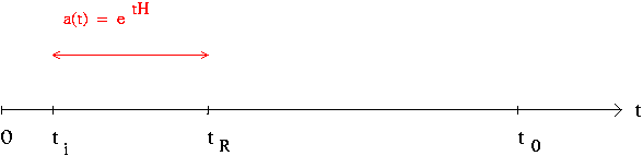
Figure 2: Time line of inflationary cosmology. The period of inflation begins at the time $t_{i}$ and ends at $t_{R}$.

In inflationary cosmology the time evolution of the horizon and of $\lambda(t)$ are modified compared to what happens in Standard Cosmology: the horizon expands exponentially in the interval between $t_{i}$ and $t_{R}$, and so does $\lambda(t)$. In contrast, the Hubble radius $l_{H}(t)$ defined as the inverse Hubble expansion rate

$$l_{H}(t)\,=\,H^{-1}(t)\,$$ (10)

is constant. Provided that the period of inflation is sufficiently long, then the horizon will at all times be larger than $\lambda(t)$ for any wavelength which can currently be observed (see Fig. 3). Thus, there is no causality problem to have homogeneity and isotropy on scales currently observed. As follows from the study of linearized fluctuations about the background (4), the Hubble radius is the upper limit on the length scales on which fluctuations can be created. From Fig. 3 it can be seen that in inflationary cosmology perturbation modes originate with a length smaller than the Hubble radius. Thus, it is possible that inflation could provide a causal mechanism for the formation of the structures which are currently observed. In fact, it turns out the quantum vacuum fluctuations in the exponentially expanding phase yield such a mechanism ChibMukh , but this is not the focus of this article (see RHBrev for a review of this topic).

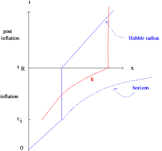
Figure 3: Space-time sketch of inflationary cosmology. The vertical axis denotes time, the horizontal axis is physical distance. During the period of inflation, the horizon expands exponentially. Similarly, the physical wavelength of a perturbation mode (the curve denoted by $k$ grows exponentially, and it is smaller than the Hubble radius at the beginning of the period of inflation, provided the period of inflation lasts sufficiently long.

In order to obtain inflationary expansion in the context of Einstein’s theory of space and time, it follows from Eqs. (FRW1) and (6) that a form of matter with

$$p\,=\,-\rho$$ (11)

is required. No such equation of state can be obtained using classical fluids, nor can it be obtained from fields representing the usual fermionic and gauge degrees of matter, at least in the context of renormalizable matter theories. Hence, a scalar field is required to obtain inflation. Even with scalar fields, it is not easy to obtain inflation since we must ensure that the potential energy density dominates over kinetic and spatial gradient energies over a long period of time. This follows from the following expressions for the energy density and pressure of scalar field matter

$$\rho\, = \,\frac{1}{2}({\dot{\varphi}})^{2}+\frac{1}{2}(\nabla\varphi)^{2}+V(\varphi)\,,$$ (12)

$$p\, = \,\frac{1}{2}({\dot{\varphi}})^{2}-\frac{1}{6}(\nabla\varphi)^{2}-V(\varphi)\,.$$ (13)

A typical potential for a scalar field which can lead to inflation is Linde

$$V(\varphi)\,=\,\frac{1}{2}m^{2}\varphi^{2}\,.$$ (14)

The equation of motion for $\varphi$ which follows from (3) is

$${\ddot{\varphi}}+3H{\dot{\varphi}}-\frac{\nabla^{2}}{a^{2}}\varphi\,=\,-V^{{}^{\prime}}(\varphi)\,,$$ (15)

where the prime indicates the derivative with respect to $\varphi$. Inflation can arise if $\varphi$ is slowly rolling, i.e. ${\ddot{\varphi}}\ll H{\dot{\varphi}}$ and ${\dot{\varphi}}^{2}\ll V(\varphi)$. Slow rolling is possible for field values $|\varphi|>m_{pl}$, where $m_{pl}$ is the Planck mass which is given by

$$m_{pl}^{2}\,=\,\bigl{(}\frac{8\pi}{3}G\bigr{)}^{-1}\,.$$ (16)

The slow roll trajectory is given by

$$\phi(t)\,=\,-\bigl{(}\frac{2}{9}\bigr{)}^{1/2}mm_{pl}t\,,$$ (17)

and it is in fact a local attractor in initial condition space for large field values Kung .

Once $|\varphi|$ drops below $m_{pl}$, the slow-roll approximation breaks down, the inflationary period ends, and $\varphi$ begins to oscillate about the minimum of its potential at $\varphi=0$. The amplitude of the oscillations is damped by the expansion of space, i.e. by the second term on the left hand side of (15).

3 The Reheating Challenge

The field $\varphi$ which leads to inflation cannot be any of the fields whose particles we have observed (except possibly the Higgs field if the latter is non-minimally coupled to gravity Shaposh ). Any regular matter (matter which is not $\varphi$) which might have been present at the beginning of the period of inflation is exponentially diluted during inflation. Thus, at the end of inflation we have a state in which no regular matter is present (the regular matter fields are in their vacuum state), and all energy is locked up in the $\varphi$ field. Thus, to make inflation into a viable model of the early universe, a mechanism is needed to convert the energy density in $\varphi$ at the end of inflation into Standard Model particles.

As was discovered in TB ; DK and worked out later in more detail in KLS1 ; STB ; KLS2 (see ABCM for a recent review) the initial energy transfer proceeds via a parametric resonance instability which is described in more generality by Floquet theory. Let us represent regular matter by a scalar field $\chi$ which is weakly coupled to $\varphi$ by an interacting term of the form

$${\cal{L}}_{I}\,=\,\frac{1}{2}g\chi^{2}\varphi\,,$$ (18)

where $g$ is a constant which has dimensions of mass. The free action for $\chi$ is assumed to be that of a canonical massless scalar field with no bare potential (i.e. no self-interactions). In this case, the equation of motion for $\chi$ becomes

$${\ddot{\chi}}+3H{\dot{\chi}}-\bigl{(}\frac{\nabla^{2}}{a^{2}}+g\varphi\bigr{)}\chi\,=\,0\,.$$ (19)

Since this is a linear differential equation, each Fourier mode $\chi_{k}$ of $\chi$ will evolve independently according to

$${\ddot{\chi}}_{k}+3H{\dot{\chi}}_{k}+\bigl{(}\frac{k^{2}}{a^{2}}-g\varphi\bigr{)}\chi_{k}\,=\,0\,.$$ (20)

After the end of the period of inflation, $\varphi$ undergoes damped oscillations. This leads to a periodic variation of the mass term in (20). This, in turn, leads to a resonant instability and to energy transfer from $\varphi$ to $\chi$.

Let us for a moment neglect the expansion of space. In this case $H=0$ and $a=1$ and then the basic matter equation (20) becomes

$${\ddot{\chi}}_{k}+\bigl{(}k^{2}-g{\cal{A}}{\rm{cos}}(\omega t)\bigr{)}\chi_{k}\,=\,0\,.$$ (21)

where ${\cal{A}}$ is the amplitude of the oscillations of $\varphi$ (constant if the expansion of space is neglected), and $\omega$ is the frequency of the oscillations (which equals $m$ in our case). Readers will recognize this equation as the Mathieu equation MathieuBook , an equation which has exponentially growing solutions in resonance bands for $k$ which are centered around half integer multiples of $\omega$. Because of this instability, there will be conversion of energy between the $\varphi$ field driving the resonance and the matter fields, as first pointed out in TB . This instabiity was later given the name “preheating” KLS1 . Since the instability is exponential, we expect that the time scale of the energy conversion is small compared to the expansion time $H^{-1}$, and that hence the approximation of neglecting the expansion of space is self-consistent.

As discussed in KLS1 ; STB ; KLS2 , the expansion of space can be included in an elegant way. In terms of a rescaled field $X_{k}=a^{3/2}\chi_{k}$, the equation of motion (20) becomes an equation of the form

$${\ddot{X_{k}}}+\Omega_{k}^{2}(t)X_{k}\,=\,0\,,$$ (22)

with an effective frequency $\Omega$ which contains a periodically oscillating term. An exponential instability persists in this setup, and this justifies the simplified approach which we focus on in this article, where we neglect the expansion of space. In the following, we will extract the periodic term from the effective frequency, i.e.

$$\Omega_{k}^{2}(t)\,=\,\omega_{k}^{2}+p(\omega t)\,.$$ (23)

Our starting equation will be

$${\ddot{\chi}}_{k}+\bigl{(}\omega_{k}^{2}+p(\omega t)\bigr{)}\chi_{k}\,=\,0\,.$$ (24)

where $\omega_{k}^{2}$ generalizes the previous setup to the case in which the $\chi$ field has a non-vanishing mass $m_{\chi}$

$$\omega_{k}^{2}\,=\,k^{2}+m_{\chi}^{2}\,,$$ (25)

and $p$ is a function with period $2\pi$. Let us denote the amplitude of $p$ by $P$. Previous work (see ABCM for a review) has shown that if $P\ll\omega^{2}$ there is “narrow-band resonance” (only $k$ modes within narrow resonance bands experience the instability), whereas if $P\gg\omega^{2}$ then there is “broad-band resonance” in which all modes with $k\ll\omega$ undergo exponential instability. In inflationary universe modes with broad-band resonance the reheating process is very rapid on Hubble time scale.

The Mathieu equation (24) is a special case of a Floquet type equation. According to Floquet theory MathieuBook ; background , the solutions of (24) scale as

$$\chi_{k}(t)\,\sim\,e^{\mu_{k}t+i\alpha_{k}t}\,,$$ (26)

where the constant $\mu_{k}+i\alpha_{k}$ is called the Floquet exponent, and the real part of it, $\mu_{k}$, is the Lyapunov exponent. The constant $\alpha_{k}$ is the rotation number of the solution, which in the context of the theory of Schrödinger operators is the “integrated density of states”.

The above setup is, however, too idealized for the purposes of real cosmology. The field $\varphi$ which yields the inflationary expansion and the field $\chi$ are only two of many fields. All of them are excited in the early universe, and they are directly or indirectly coupled to $\chi$, and they will hence give correction terms to the basic equation (24). The extra fields are called the “environment” in which the system under consideration lives. The environment is typically describeable by random noise, which is uncorrelated in time with the time-dependence of $\varphi(t)$. We will now consider an idealized equation which includes effects of the noise:

$${\ddot{\chi}}+\bigl{(}-\nabla^{2}+p(\omega t)+q(x,t)\bigr{)}\chi\,=\,0\,.$$ (27)

where $q(x,t)$ is a stochastic variable whose time-dependence is uncorrelated with that of $\varphi(t)$.

4 Homogeneous Noise

Our basic equation (27) is a second order partial differential equation with random coefficients. In phase space, we obtain a random matrix equation which is first order in time.

To simplify the analysis, we will first consider the case of homogeneous noise, i.e. we will assume that the noise function $q$ depends only on time. In this case, each Fourier mode of $\chi$ continues to evolve independently and satisfies the equation

$${\ddot{\chi}}_{k}+\bigl{(}k^{2}+p(\omega t)+q(t)\bigr{)}\chi\,=\,0\,.$$ (28)

This dramatically reduces the mathematical complexity of the problem: we now have a second order ordinary differential equation rather than a PDE.

To re-write this equation in the form of a random matrix equation we introduce the transfer matrix $\Phi_{q}(t,0)$ made up of two independent solutions $\phi_{1}(t;q)$ and $\phi_{2}(t;q)$ of (28) and their time derivatives:

$$\Phi_{q}(t,0)\,=\,\left(\begin{array}[]{cc}\phi_{1}(t;q)&\phi_{2}(t;q)\\ {\dot{\phi_{1}}}(t;q)&{\dot{\phi_{2}}}(t;q)\end{array}\right).$$

which satisfies the first order matrix equation

$${\dot{\Phi_{q}}}\,=\,M(q(t),t)\Phi_{q}\,,$$ (29)

where the matrix $M$ is given by

$$M\,=\,\left(\begin{array}[]{cc}0&1\\ -(\omega_{k}^{2}+p+q)&0\end{array}\right).$$

The transfer matrix describes the evolution of the system from initial time $t=0$ to final time $t$.

Let us denote the transfer matrix in the absence of noise by $\Phi_{0}(t,0)$. According to Floquet theory (see e.g MathieuBook ; background ) for mathematical background), this matrix takes the form

$$\Phi_{0}(t,0)\,=\,P_{0}(t)e^{Ct}\,$$ (30)

where $P_{0}(t)$ is a periodic matrix function with period $\omega^{-1}$, and $C$ is a constant matrix whose spectrum is

$${\rm{spec}}(C)\,=\,\{\pm\mu(0)\}\,,$$ (31)

where $\mu(0)$ is called the Lyapunov exponent in the absence of noise.

To study the effects of noise, we re-write the full transfer matrix by extracting the transfer matrix in the absence of noise:

$$\Phi_{q}(t,0)\,=\,\Phi_{0}(t,0)\Psi_{q}(t,0)\,,$$ (32)

where the non-triviality of the reduced matrix $\Psi$ describes the effects of the noise. The reduced transfer matrix satisfies the equation

$${\dot{\Psi}}_{q}\,=\,S\Psi_{q}\,,$$ (33)

where $S$ is the following matrix:

$$S\,=\,\Phi_{0}^{-1}\left(\begin{array}[]{cc}0&0\\ -q&0\end{array}\right)\Phi_{0}\,.$$

Let $T$ be the period of the oscillation of $\phi$. We can now write the transfer matrix as a product of transfer matrices over individual oscillation times:

$$\Phi_{q}(NT,0)\,=\,\prod_{j=1}^{N}\Phi_{q}(jT,(j-1)T)\,,$$ (34)

where $N$ is an integer.

Let us assume that the noise is uncorrelated in time when considered in different oscillation periods. In addition, let us assume that the noise is drawn from some probability measure on ${\cal{C}}({\cal{R}})$ such that $q$ restricted to a period fills a neighborhood of ${\cal{C}}({\cal{R}})$. In this case, the overall Lyapunov exponent is well defined and can be extracted using the limit Craig1

$$\mu(q)\,=\,{\rm{lim}}_{N\rightarrow\infty}\frac{1}{NT}{\rm{log}}||\prod_{j=1}^{N}\Phi_{q}(JT,(j-1)T)||\,,$$ (35)

where $\|\cdot\|$ indicates a matrix norm. Note that the dependence on the particular matrix norm vanishes in the limit $N\rightarrow\infty$.

The key result of Craig1 is that noise which obeys the above-mentioned conditions renders the instability stronger. More specifically, we have the following theorem:

Theorem 4.1

Given a random noise function $q(t)$ which is uncorrelated on the time scale $T$ and which is drawn from a probability measure on ${\cal{C}}({\cal{R}})$ such that $q$ restricted to a period fills a neighborhood of ${\cal{C}}({\cal{R}})$, then

$$\mu(q)\,>\,\mu(0)\,.$$ (36)

Note the strict inequality in the above theorem. At first sight, this result could be surprising since one might expect that noise could cut off an instability which occurs in the absence of noise. However, a physical way to understand the result of the above theorem is to realize that the noise we have introduced can only add energy to the system rather than drain energy. Thus, it is consistent to find that noise renders the resonant instability more effective.

The above theorem follows from the Furstenberg Theorem Furstenberg on random matrices. This theorem takes the following form:

Theorem 4.2

Given a probability distribution $dA$ on $\Psi\in SL(2n,{\cal{R}})$ and defining $G_{A}$ as the smallest subgroup of $SL(2n,{\cal{R}})$ containing the support of $dA$, then if $G_{A}$ is not compact, and $G_{A}$ restricted to lines has no invariant measure, then for almost all independent random sequences $\{\Psi_{j}\}_{j=1}^{\infty}$ distributed according to $dA$ we have

$${\rm{lim}}_{N\rightarrow\infty}\frac{1}{N}{\rm{log}}||\prod_{j=1}^{N}\Psi_{j}||\,=\,\lambda\,>\,0\,.$$ (37)

In addition, for almost all vectors $v_{1}$ and $v_{2}$ in ${\cal{R}}^{2n}$ the exponent $\lambda$ can be extracted via

$$\lambda\,=\,{\rm{lim}}_{N\rightarrow\infty}\frac{1}{N}{\rm{log}}<v_{1},\prod_{j=1}^{N}\Psi_{j}v_{2}>\,.$$ (38)

Note once again the strict inequality in the above theorem. Applied to our reheating problem, then for any mode $k$, the above theorems in the case of $n=1$ can be used, and they imply that, in the presence of noise, the Floquet exponent increases for each value of $k$. In particular, if for a particular value of $k$ there is no instability in the absence of noise, an instability will develop in the presence of noise.

The way that our result (36) follows from Furtsenberg’s Theorem is the following. Let us take $v_{1}$ to be an eigenvector of $\Phi_{0}(T,0)^{t}$, the transverse of the noiseless transfer matrix with eigenvalue $exp(\mu(0)T)$. Then,

$$\mu(q)\, = \,{\rm{lim}}_{N\rightarrow\infty}\frac{1}{NT}{\rm{log}}\bigl{(}<v_{1},\Phi_{q}(NT,0)v_{2}>\bigr{)}$$ (39)

$$= \,{\rm{lim}}_{N\rightarrow\infty}\frac{1}{NT}{\rm{log}}\bigl{(}e^{\mu_{0}NT}<v_{1},\prod_{j=1}^{N}\Psi_{j}(jT,(j-1)T)v_{2}>\bigr{)}$$

$$= \,\mu(0)+\lambda\,>\,\mu(0)\,,$$

where in the last step we have used Furstenberg’s Theorem.

From the point of view of physics, the restriction to homogeneous noise is not realistic. We must allow for inhomogeneous noise functions $q(x,t)$. This is the topic we turn to in the following section.

5 Inhomogeneous Noise

In the case of inhomogeneous noise we must return to the original partial differential equation (27) with random noise. By going to phase space we obtain a first order matrix operator differential equation

$${\dot{\Phi_{q}}}\,=\,M(q(t,\cdot),t)\Phi_{q}$$ (40)

for the fundamental solution matrix operator $\Phi_{q}$. The Floquet exponent for the inhomogeneous system is defined by

$$\mu_{q}\,=\,{\rm{lim}}_{N\rightarrow\infty}{\rm{log}}||\Phi_{q}(NT,0)||\,,$$ (41)

where, as before, $||$ indicates a norm on the matrix operator space, and $T$ is the period of the unperturbed system.

As in the previous section, we will separate out the effects of the noise by defining

$$\Phi_{q}(t)\,=\,\Phi_{q=0}(t)\Psi_{q}(t)\,,$$ (42)

where $\Phi_{q=0}$ is the fundamental solution matrix in the absence of noise, and $\Psi_{q}(t)$ is the matrix which encodes the effects of the random noise. We wish to compare the value of the Floquet exponent in the presence of noise with that of the noiseless system.

To dramatically reduce the complexity of the problem we apply a trick which is commonly used is physics. First, we introduce an infrared cutoff by replacing the infinite spatial sections ${\cal{R}}^{3}$ by a three-dimensional torus of side length $L$. This renders Fourier space discrete. Secondly, we impose an ultraviolet cutoff, namely we eliminate high “energy” modes with $k<\Lambda$, where $\Lambda$ is the cutoff scale. The fundamental solution matrix of the cutoff problem is denoted by $\Phi_{q}^{L,\Lambda}(t)$, and the corresponding Floquet exponents are also denoted by superscripts.

After the above steps, our problem can be written in Fourier space as a ordinary matrix differential equation in ${\cal{R}}^{2n}$, where $n$ is the number of Fourier modes which are left. The first pair of coordinates corresponds to the phase space coordinates of the first Fourier mode and so forth. In the absence of noise, the fundamental solution matrix is block diagonal - there is no mixing between different Fourier modes. In each block, $\Phi_{q=0}^{L,\Lambda}$ reduces to the transfer matrix of the corresponding Fourier mode discussed in the previous section. The noise term $\Psi_{q}$ introduces mixing between the different blocks.

Since Furstenberg’s Theorem is valid on ${\cal{R}}^{2n}$, the results of the previous section immediately apply and we have

$$\mu_{q}^{L,\Lambda}\,>\,\mu_{0}^{L,\Lambda}\,.$$ (43)

Note the fact that we have a strict inequality. Note also that the Floquet exponent in the noiseless case is the maximum of the Floquet exponents over all values of $k$:

$$\mu_{0}^{L,\Lambda}\,=\,{\rm{max}}_{k}(\mu_{k,0})\,,$$ (44)

where $\mu_{k,0}$ is the Floquet exponent for Fourier mode $k$ in the absence of noise.

Let us now consider removing the limits, i.e. taking $L\rightarrow\infty$ and $\Lambda\rightarrow\infty$. Since in the absence of noise, there is no resonance for large $k$ modes, the limit of the right hand side of (43) is well defined (in fact, the right hand side is independent of the cutoffs). For any finite value of the cutoffs, the result (43) is true. Hence, the result persists in the limit when the cutoffs are taken to infinity. However, one loses the strict inequality sign. Hence, assuming that the limit of the left hand side of (43) in fact exists, we obtain our final result

$$\mu_{q}\,\geq\,{\rm{max}}_{k}(\mu_{k,0})\,.$$ (45)

We in fact expect a stronger result. Let us denote by $\mu_{q}(k)$ the Floquet exponent of the dynamical system restricted to the k’th Fourier mode (the restriction made at the end of the evolution). Then we expect that due to the mode mixing the maximal growth rate over all Fourier modes of the noiseless system will influence all Fourier modes of the system with noise, and that hence

$$\mu_{q}(k)\,\geq\,{\rm{max}}_{k}(\mu_{k,0})\,.$$ (46)

Although we have numerical evidence Craig2 for the validity of this result, we have not been able to provide a proof.

6 New Proof of Anderson Localization

It is well known that there is a correspondence between classical time-dependent problems and a time-independent Schrödinger equation. Let us start from the second order differential equation (28) in the case of homogeneous noise. Let us now make the following substitutions:

$$\chi\, \rightarrow \,\psi$$

$$t\, \rightarrow \,x$$

$$\omega_{k}^{2}\, \rightarrow \,2mE$$ (47)

$$p(\omega t)\, \rightarrow \,-2mV_{p}(\omega x)$$

$$q(t)\, \rightarrow \,-2mV_{R}(x)\,.$$

Then, the equation (28) becomes

$$H\psi\,=\,E\psi\,,$$ (48)

with the operator $H$ given by

$$H\,=\,-\frac{1}{2m}\frac{\partial^{2}}{\partial x^{2}}+V_{p}(\omega x)+V_{q}(x)\,,$$ (49)

which is the time-independent Schrödinger equation for the wavefunction $\psi$ of an electron of mass $m$ in a periodic potential $V_{p}(\omega x)$ of period $\omega^{-1}$ in the presence of a random noise term $V_{R}$ in the potential.

In the absence of noise there are bands of values of $E$ where there is no instability, and where hence the wave functions are oscillatory. In condensed matter physics, the corresponding solutions for $\psi$ are known as Bloch wave states. Theorem 1 now implies that if a random potential is added, then the solutions for $\psi$ become unstable. This means that there is one exponentially growing mode and one exponentially decaying mode. In quantum mechanics the growing mode is unphysical since it is not normalizable. Hence, the decaying mode is the only physical mode. This solution corresponds to a localized wave function. Thus, we have obtained a new proof of the finiteness of the localization length in the theory of “Anderson localization” Anderson (for reviews see e.g. Revs )

Theorem 6.1

Consider the time-independent Schrödinger equation for a particle in a periodic potential $V_{p}(\omega x)$, and consider a random noise contribution $V_{q}(x)$ which is uncorrelated on the length scale of the period of $V_{p}$ and which is drawn from a probability measure on ${\cal{C}}({\cal{R}})$ such that $q$ restricted to a period fills a neighborhood of ${\cal{C}}({\cal{R}})$. Then the presence of the noise localizes the wavefunction, and the localization strength is exponential, i.e. the wavefunction $\psi_{q}$ in the presence of noise scales as

$$\psi_{q}(x)\,\sim\,exp(-\mu(q)x)\,.$$ (50)

where $\mu(q)$ is strictly positive on the basis of Theorem 1.

Note that our method can only be applied to study Anderson localization in one spatial dimension.

7 Conclusions

We have applied rigorous results from random matrix theory to study the effects of noise on reheating in inflationary cosmology. We have found that the type of noise studied here, namely a random noise contribution to the mass term in the Klein-Gordon equation for a scalar field representing Standard Model matter, renders the parametric resonance instability of matter production in the presence of an oscillating inflaton field more effective. After the standard duality mapping between a time-dependent classical field theory problem and a time-independent quantum mechanical Schrödinger problem, we obtain a new proof of the finiteness of the localization length in the theory of “Anderson localization”, a famous result in condensed matter physics. Our work is an example of how the same rigorous mathematics result can find interesting applications to diverse physics problems.