HEP preprint-july-2014
Geometry of the Ground State of Higgs Fields in Next-to-MSSM

Abstract

Decomposing the Higgs potential $\mathcal{V}_{higgs}$ of next - to - Minimal Supersymmetric Standard Model (n-MSSM)  as the sum of three contributions like $\mathcal{V}_{ch}+\mathcal{V}_{kah}+\mathcal{V}_{expl}$ and assuming the two following things: $\left(a\right)$ $\mathcal{V}_{higgs}$ dominated by $\mathcal{V}_{ch}$ coming from the chiral sector of supersymmetry: $\mathcal{V}_{ch}=\left|\mathrm{\nu}\right|^{2}\mathcal{U}$ with $\left|\mathrm{\nu}\right|$ large and $\frac{\mathrm{r}}{\left|\mathrm{\nu}\right|}<<1$; and $\left(b\right)$ replacing the chiral down Higgs superfield doublet $\left(\boldsymbol{H}_{d}\right)^{i}$ of n-MSSM by a chiral anti-doublet $\left(\boldsymbol{\Phi}_{d}\right)_{i}$; we derive the explicit geometry of the Higgs fields in the ground state $\left|\Sigma_{higgs}\right\rangle$ found to be given by two intersecting conifolds. We show as well that the property $\tan\beta_{susy}=1$ living at singularity $r=0$ is a supersymmetric signal; and deviation away reads in terms of the Kahler parameter $r$ and the $\vartheta_{{}_{W}}$- Weinberg angle as $\tan\beta\simeq 1+\frac{\mathrm{r}}{2\left|\mathrm{\nu}\right|}\sin^{2}\vartheta_{{}_{W}}$. Other related issues are also studied.

1 Introduction

The experimental discovery of a Higgs-like particle with a mass $M_{h}\simeq 126$ $GeV$ is a great success of the $SU_{L}\left(2\right)\times U_{Y}\left(1\right)$ standard model (SM) of electroweak unification A1 ; A2 . After three decades since the obtention of the W^± and Z⁰ gauge particles, the recent observation of a Higgs-like constitutes another big step towards understanding the architecture of elementary particles and their interactions around the electroweak scale. This discovery also opens a window on exploration of extended candidates of SM among which supersymmetric theories; in particular the Minimal Supersymmetric Standard Model (MSSM) B1 -B9 and extensions such as the next - to - MSSM extension C1 -C12 we are interested in here in this study.

Motivated by the LHC experimental breakthrough, and by the basic role played by the Higgs fields that capture data on ground state of standard model and on masses of its particles, we focus in this paper on the Higgs sector of the next -to- MSSM in superspace ( shortly n-MSSM) and study the following points:

$1)$

The effect of putting a chiral anti-doublet $\Phi_{\bar{\imath}}$ at the place of the chiral superfield doublet $\boldsymbol{H}_{d}^{i}$; but the others Higgs superfields $\boldsymbol{H}_{u}^{i}$ and $\boldsymbol{S}$ unchanged; that is modifying the quantum numbers of the Higgs chiral superfields of n-MSSM like
                

                n-MSSM $$\rightarrow$$                      n-MSSM^∗

doublet : doublet :

doublet : anti-doublet :

singlet : singlet :

(1)

This quantum number change of the down Higgs superfield is manifested at the interaction level between $\boldsymbol{\Phi}_{\bar{\imath}}$ and the non abelian gauge superfields by a change of the sign of the $SU_{L}\left(2\right)$ gauge coupling constant $g_{su_{2}}$ ( see eqs 113). It has been motivated by the opposite hypercharges of $\boldsymbol{H}_{u}^{i}$ and $\boldsymbol{H}_{d}^{i}$ under $U_{Y}\left(1\right)$ symmetry transformations; and also by (a) and (b) given here below:
            
$\left(\mathbf{a}\right)$ the seeking for a non trivial geometric interpretation of the Higgs ground state $\left|\Sigma\right\rangle$ in terms of intersecting manifolds; this property is indicated by the superspace lagrangian density of n-MSSM; the 4 chiral superfields $\boldsymbol{\Phi}_{i}$ and $\boldsymbol{H}_{u}^{i}$ obey the typical complex 3D conifold relations:

$$\ \ \ \ \ \ \ \ \ \ \ \ \boldsymbol{\Phi}_{i}\boldsymbol{H}_{u}^{i}$$ :

:

showing that Higgs fields ground state lives on the intersection of the threefolds $\mathfrak{C}_{\nu}$ and $\mathfrak{R}_{r}$ given by a complex surface $\mathcal{S}$; see eqs (115). The other constraints on $\boldsymbol{\Phi}_{i}$ and $\boldsymbol{H}_{u}^{i}$, coming from the minimization of the scalar potential, give extra data on the precise location of the Higgs VEVs within the surface $\mathcal{S}$.

$\left(\mathbf{b}\right)$ exhibiting explicitly the dual role of the component scalar Higgs fields $\boldsymbol{h}_{u}$ and $\boldsymbol{h}_{d}$; seen that one Higgs doublet, say $\boldsymbol{h}_{u}$, is sufficient to break $SU_{L}\left(2\right)\times U_{Y}\left(1\right)$ gauge symmetry down to $U_{em}\left(1\right)$. This duality, which is understood in n-MSSM, is precisely given by the relation $\boldsymbol{\Phi}_{i}\boldsymbol{H}_{u}^{i}=\mathrm{\nu}$ and remarkably captured by the extra chiral singlet superfield $\boldsymbol{S}$ of n-MSSM.

$2)$

The underlying geometry of the quantum phases of the Higgs ground state namely the supersymmetric phase $\left|\Sigma_{susy}\right\rangle$ and the non supersymmetric one $\left|\Sigma_{n-susy}\right\rangle$. We first study the structure of these geometries, given by compact complex curves inside the surface $\mathcal{S}$, respectively denoted as $\Sigma_{susy}$ and $\Sigma_{n-susy}$; and then derive the explicit expression of their metrics as well as specific properties. In the first case, we show amongst others that the ratio $\frac{\upsilon_{h}}{\upsilon_{d}}$ of the Higgs VEVs corresponds exactly to

$$\tan\beta_{susy}=1$$

and in the case of $\Sigma_{n-susy}$, we find that this ratio deviates from unity as

$$\tan\beta=\frac{\mathrm{r}\sin^{2}\vartheta_{{}_{W}}}{2\left|\mathrm{\nu}\right|}+\sqrt{1+\left(\frac{\mathrm{r}\sin^{2}\vartheta_{{}_{W}}}{2\left|\mathrm{\nu}\right|}\right)^{2}}$$

with $\left|\frac{\mathrm{r}}{\mathrm{\nu}}\right|<<1$ and r a real number; non necessary positif. We find moreover that the metric of $\Sigma_{n-susy}$ reads in terms of the $\vartheta_{{}_{W}}$- Weinberg angle like

$$ds_{\Sigma_{\text{n-susy}}}^{2}=\frac{1}{4}\mathcal{R}_{{}_{H}}^{2}\left(d\theta^{2}+4\cos^{2}\frac{\theta}{2}d\phi^{2}\right)$$ (2)

with $\theta$ and $\phi$ standing for the usual coordinates of the real 2-sphere, and the radius $\mathcal{R}_{H}$ given by

$$\mathcal{R}_{{}_{H}}^{2}=\frac{2\left|\mathrm{\nu}\right|^{2}+\mathrm{r}^{2}\sin^{2}\vartheta_{{}_{W}}+\mathrm{r}\sqrt{4\left|\mathrm{\nu}\right|^{2}+\mathrm{r}^{2}\sin^{4}\vartheta_{{}_{W}}}}{\mathrm{r}^{2}\sin^{2}\vartheta_{{}_{W}}+\sqrt{4\left|\mathrm{\nu}\right|^{2}+\mathrm{r}^{2}\sin^{4}\vartheta_{{}_{W}}}}$$

From this point of view, the real Fayet Iliopoulos (FI) coupling constant $\mathrm{r}\sim M^{2}$ may be then thought of as given by the mass scale where supersymmetry breaks down. In other works, if taking the high energy limit $\frac{\mathrm{r}}{\left|\mathrm{\nu}\right|}=0$, the squared radius tends to $\left.\mathcal{R}_{{}_{H}}^{2}\right|_{\mathrm{r}=0}=\left|\mathrm{\nu}\right|$ and one is left with the supersymmetric phase $\left|\Sigma_{\text{susy}}\right\rangle$.
     
Furthermore, we find that the point $\mathcal{P}_{u_{{\small em}}{\small(1)}}$, where the $SU_{L}\left(2\right)\times U_{Y}\left(1\right)$ gauge symmetry breaks spontaneously down to $U_{em}\left(1\right)$, sits in our geometric description, at the south pole

$$\theta=\pi$$

of the real 2-sphere (2) where the metric degenerates and the "electromagnetic" circle $\mathbb{S}_{em}^{1}$, parameterized by the angle $\phi$, shrinks to $\mathcal{P}_{u_{{\small em}}{\small(1)}}$.
       
We also derive the following formula for the energy density of the non supersymmetric ground state $\left|\Sigma_{\text{n-susy}}\right\rangle$

$$\mathcal{E}_{\min}=\mathcal{E}_{0}+\frac{\sin^{2}\left(2\vartheta_{{}_{W}}\right)}{32}\mathrm{r}^{4}$$

with the constant $\mathcal{E}_{0}$ related to explicit supersymmetry breaking.

The presentation of this paper is as follows: In section 2, we present the key idea of our proposal; describe the method of approaching the solutions of non linear coupled equations; and give a summary of main results obtained in this work. In section 3, we review basic aspects on the quantum charges of the Higgs fields under the $SU_{L}\left(2\right)\times U_{Y}\left(1\right)$ gauge symmetry and develop our proposal regarding the $SU_{L}\left(2\right)$ gauge charge of the Higgs doublet $H_{d}$. In our method, we replace the chiral superfield doublet $H_{d}^{i}$ by an anti-doublet $\Phi_{i}$ whose $SU_{L}\left(2\right)\times U_{Y}\left(1\right)$ quantum charges, including those of $SU_{L}\left(2\right)$, are given by the opposite of those of $H_{u}$. In section 4, we study the superfield formulation of n-MSSM; but by using the anti-doublet $\Phi_{i}$ at the place of $H_{d}^{i}$. In section 5, we consider the case $r=0$; while letting the complex $\nu$ arbitrary; and study the set of exact solutions of the auxiliary field’s equations of motion; their intersections as well as the phase of ground state. In section 6, we switch on the real FI coupling constant $r\neq 0$ and examine the solution of the equations of motion of the auxiliary fields. In this case, we show that supersymmetry is broken and we determine the energy density of the ground state as well as the deviation of the $\tan\beta$ ratio of the Higgs VEVs. In section 7, we explore general aspects of explicit supersymmetry breaking and in section 8, we give a conclusion and make some comments. Sections 9 and 10 are respectively devoted to appendices on useful tools on next - to -MSSM and the metric of the intersecting conifold geometry.

2 n-MSSM* and summary of results

In this section, we draw the main lines behind n-MSSM* of table (1) and give a summary of some of the results obtained in this study; technical details and other results are exposed in the forthcoming sections and in the two appendices.

2.1 General on n-MSSM in superspace

We begin by recalling useful ingredients on supersymmetric gauge theories in superspace taking as an example the next -to- MSSM extension of $U_{Y}\left(1\right)\times SU_{L}\left(2\right)$ standard model; and focussing on Higgs sector and interactions with gauge radiation.

Quantum charges of n-MSSM Higgs
Next -to- MSSM extension of standard model involves 5 Higgs chiral superfields: a hyperchargeless iso-singlet $\boldsymbol{S}$ and two doublets $\boldsymbol{H}_{u}=\left(H_{u}^{+},H_{u}^{0}\right)$ and $\boldsymbol{H}_{d}=\left(H_{d}^{0},H_{d}^{-}\right)$ with opposite hypercharge, $y_{u}=-y_{d}=1$; but same charge under $SU_{L}\left(2\right)$. A way to see how these quantum charges are manifested in the lagrangian density $\mathcal{L}$ of the model is through the gauge covariant derivatives of the leading scalar field components $S$, $\left(h_{u}^{i}\right)$ and $\left(h_{d}^{i}\right)$ of the chiral superfields $\boldsymbol{S}$, $\boldsymbol{H}_{u}$ and $\boldsymbol{H}_{d}$. While $\partial_{\mu}S$ is un-affected under gauge symmetry transformations, $\left(\partial_{\mu}h_{u}\right)^{i}$ and $\left(\partial_{\mu}h_{d}\right)^{i}$ get modified into gauge covariant derivatives $\left(\nabla_{\mu}h_{u}\right)^{i}$ and $\left(\nabla_{\mu}h_{d}\right)^{i}$ depending on the bosonic gauge fields $B_{\mu}$ and $W_{\mu}^{A}$ as given below

$$\left(\nabla_{\mu}h_{u}\right)^{i}$$

(3)

These gauge covariant derivatives differ only by the sign of the $U_{Y}\left(1\right)$ gauge coupling constant $g^{\prime}$; this is because the Higgs fields $h_{u}^{i}$ and $h_{d}^{i}$ have opposite hypercharges; but the same $SU_{L}\left(2\right)$ charge,

$$\left[Y,h_{u}^{i}\right]$$ ,

,

(4)

where $Y$ and $T^{A}$ are the hermitian generators of the $U_{Y}\left(1\right)\times SU_{L}\left(2\right)$ gauge symmetry. Later on, we consider as well a gauge covariant derivative $\mathcal{D}_{\mu}\varphi_{i}$ of the anti-doublet $\varphi_{i}$ where the sign of both gauge couplings $g^{\prime}$ and $g$ of the $U_{Y}\left(1\right)$ and $SU_{L}\left(2\right)$ gauge symmetry factors are flipped; see eq(26) for comparison and to fix the idea.

Scalar potential $\mathcal{V}_{sca}$   
In supersymmetric gauge theories describing the interacting dynamics between supersymmetric chiral matter and supersymmetric gauge multiplets, the scalar potential energy density $\mathcal{V}_{sca}$ is positive and is given by the sum of two basic terms

$$\mathcal{V}_{sca}=\mathcal{V}_{ch}+\mathcal{V}_{re}\geq 0$$ (5)

with $\mathcal{V}_{ch}$ and $\mathcal{V}_{re}$ describing respectively the contribution coming from the auxiliary fields $F$ (depending on chiral superpotential) and the auxiliary fields $D$ (Kahler sector).
In the case of n-MSSM, the potential energy densities $\mathcal{V}_{ch}$ and $\mathcal{V}_{re}$ read as

$$\mathcal{V}_{ch}$$

(6)

The term $\mathcal{V}_{ch}$ is the sum of 5 quadratic monomials in one one to one with the number of the 5 Higgs chiral superfields $\boldsymbol{S}$, $\boldsymbol{H}_{u}^{i}$ and $\boldsymbol{H}_{d}^{i}$ and so with the number of bosonic Higgs fields $S$, $\left(h_{u}^{i}\right)$ and $\left(h_{d}^{i}\right)$. The potential $\mathcal{V}_{ch}$ depends moreover on the complex coupling constants $\left\{\lambda_{x},\bar{\lambda}_{x}\right\}$ of the intra superfield Higgs interactions; typically

$$W=\lambda\boldsymbol{SH}_{u}\boldsymbol{H}_{d}+\nu\boldsymbol{S}+\frac{\kappa}{3}\boldsymbol{S}^{3}$$ (7)

Similarly, the term $\mathcal{V}_{re}$ is given by the sum of 4 quadratic monomials in one to one with the 4 gauge multiplets $\boldsymbol{V}^{\prime}$ and $\boldsymbol{V}^{A}$ of the $U_{Y}\left(1\right)\times SU_{L}\left(2\right)$ gauge symmetry group. It depends on the real gauge coupling constants $g$ and $g^{\prime}$; but not on $\left\{\lambda_{x},\bar{\lambda}_{x}\right\}$.

To deal with the total scalar potential in n-MSSM, one first uses the equations of motion of the auxiliary fields to get the expressions of the F’s and the D’s in terms of the bosonic scalar fields $S$, $h_{u}^{i},$ $h_{d}^{i}$. Generally, these are quadratic quantities in the Higgs fields; and so the scalar potential

$$\mathcal{V}=\mathcal{V}_{{\small n}\text{{\small-}}MSSM}+\mathcal{V}_{exl}$$

is a quartic polynom in $S$, $h_{u}^{i},$ $h_{d}^{i}$ bounded from below; with sections having generally 3 extrema: 2 minima and a local extremum.
Then one determines the set of Higgs configurations that minimize the total scalar potential

$$\mathcal{V}\left(h_{u},h_{d},S,\text{ }\bar{h}_{u},\bar{h}_{d},\bar{S}\right)$$

to get the ground state $\left|\Sigma_{Higgs}\right\rangle$ of the Higgs fields.
If thinking about $\mathcal{V}$ as the mapping

$$\mathcal{V}$$

the ground state $\Sigma_{Higgs}$ of the 5 complex Higgs field $h_{u},h_{d},S$ lives then inside of $\mathbb{C}^{5}$ and is given by the kernel of $\mathrm{\delta}_{var}\mathcal{V}$; the variation of the total scalar potential with respect to the 5 Higgs fields,

$$\Sigma_{Higgs}=\ker\left(\mathrm{\delta}_{var}\mathcal{V}\right)\subset\mathbb{C}^{5}$$ (8)

This set is completely characterized by the two real gauge couplings constants $g$ and $g^{\prime}$; as well as by the complex coupling constants $\left\{\lambda_{\left\{x\right\}},\bar{\lambda}_{\left\{x\right\}}\right\}$ of the intra Higgs interactions including those coming from the explicit supersymmetry breaking terms; see eq(168) and section 7 as well as appendix A for further details.

2.2 The proposed n-MSSM* and first results

Motivated by the determination of the three followings:

• the topological shape of the Higgs manifold $\Sigma_{Higgs}$ associated with Higgs ground state,

• the explicit expression of the metric $ds_{\Sigma}^{2}$ of $\Sigma_{Higgs}$; and

• the property of $ds_{\Sigma}^{2}$ that singles out the electrically neutral point $P_{u_{1}^{em}}\in\Sigma_{Higgs}$ where $U_{Y}\left(1\right)\times SU_{L}\left(2\right)$ symmetry breaks down to $U_{em}\left(1\right)$,

we consider in this study the Higgs sector of n-MSSM on which we impose two assumptions that allow very explicit calculations and permit more insight into the structure $\Sigma_{Higgs}$.

$\mathbf{a})$ assumption I: $\mathcal{V}_{ch}>>\mathcal{V}_{re}+\mathcal{V}_{exl}$
the total the scalar potential $\mathcal{V}$ is dominated by the contribution coming from the chiral sector of supersymmetry; this property fixes the topological shape of the manifold where lives $\Sigma_{Higgs}$,

$\mathbf{b})$ assumption II: n-MSSM  $\rightarrow$    n-MSSM^∗
the two chiral Higgs doublet superfields are assumed to be dual superfields; in the sense they have opposite quantum numbers; i.e: they have opposite $U_{Y}\left(1\right)$ hypercharges and also opposite $SU_{L}\left(2\right)$ ones.
With this some how natural assumption, one expects that the self dual point to be a critical point of $ds_{\Sigma}^{2}$ where a phase transition takes place; As we will see later self dual point corresponds precisely to the supersymmetric phase.

The first hypothesis is further explored in sub-sub- section 2.2.1 and the second one is studied in sub-sub- section 2.2.2.

2.2.1 More on the condition $\mathcal{V}_{ch}>>\mathcal{V}_{re}+\mathcal{V}_{exl}$

First, notice that from the explicit expression of the total scalar potential

$$\mathcal{V} = \mathcal{V}_{susy}+\mathcal{V}_{exl}$$

$$= \left(\mathcal{V}_{ch}+\mathcal{V}_{re}\right)+\mathcal{V}_{exl}$$

one learns that in order to determine the set $\Sigma_{Higgs}$ of eq(8) one has to solve the 5 complex equations

$$\frac{\partial\mathcal{V}}{\partial S}$$

(9)

and look for their intersecting solutions. Clearly this system of complex equations has solutions; but difficult to figure out explicitly due to the number of relations; their couplings as well as the cubic non linearities in the field variables.

1) the condition on scalar potential
In order to get explicit solutions of the above relations, we make the hypothesis

$$\mathcal{V}_{ch}>>\mathcal{V}_{re}+\mathcal{V}_{exl}$$

which should be thought of as corresponding to a particular region in the moduli space of coupling constants of n-MSSM. In fact this region corresponds to high energy limit where lives the supersymmetric phase of the model.
With this condition, one may think about the total scalar potential of the model as mainly given by $\mathcal{V}_{ch}$ with a perturbation $\mathrm{\delta}_{pert}\mathcal{V}=\mathcal{V}_{pert}$ equal to $\left(\mathcal{V}_{re}+\mathcal{V}_{exl}\right)$. Explicitly,

$$\mathcal{V}=\mathcal{V}_{ch}+\mathcal{V}_{pert}$$ (10)

with

$$\mathcal{V}_{pert}=\frac{1}{2}\left(D^{\prime}\right)^{2}+\frac{1}{2}\mathop{\displaystyle\sum}\limits_{A=1}^{3}D_{{\small A}}D^{{\small A}}+\mathcal{V}_{exl}$$ (11)

Then use the approximation to compute explicitly the ground state $\left|\Sigma\right\rangle$ and its phases by proceeding as follows:

• First, compute the minimum of $\mathcal{V}_{ch}=\sum_{I}\bar{F}_{I}F^{I}$ obtained by solving the condition

  $$\delta\mathcal{V}_{ch}=\mathop{\displaystyle\sum}\limits_{I}\bar{F}_{I}\left(\delta F^{I}\right)+F^{I}\left(\delta\bar{F}_{I}\right)=0$$

  and remarkably given by the zero energy condition

  $$\mathcal{V}_{ch}=\bar{F}_{ui}F_{u}^{i}+\bar{F}_{di}F_{d}^{i}+\bar{F}_{S}F_{S}=0$$ (12)

  or equivalently

  $$\bar{F}_{S}$$

  (13)

  The explicit expression of the solutions of these relations are a priori not difficult to obtain seen that they are quadratic in the Higgs fields; let us denote these solutions as

  $$\left\langle S\right\rangle,$$

  (14)

  and refer to them collectively as $\xi$; they parameterize a submanifold $\mathfrak{C}_{\nu}$ in $\mathbb{C}^{5}$.

• Then, put these solutions back into the total scalar potential $\mathcal{V}$, we get the following hermitian function depending on the $\xi$ moduli

  $$\mathcal{V}\left(\xi\right)$$

  (15)

  because $\mathcal{V}_{ch}\left(\xi\right)=0$.

• Next, compute the minimum of

  $$\mathcal{V}_{pert}=\mathcal{V}_{re}\left(\xi\right)+\mathcal{V}_{exl}\left(\xi\right)$$

  to end with the values of the Higgs fields minimizing the potential energy density; and which we denote like,

  $$\xi_{\min}=\left\{\left\langle S\right\rangle_{\min},\left\langle h_{u}^{i}\right\rangle_{\min},\ \left\langle h_{d}^{i}\right\rangle_{\min}\right\}$$

  The set of these minima gives the ground state $\left|\Sigma\right\rangle$ of the Higgs fields.
                          
  Clearly, the geometry of the Higgs ground state $\Sigma_{\nu}$ depends on $\mathcal{V}_{ch}\left(\xi\right)$, $\mathcal{V}_{re}\left(\xi\right)$ and $\mathcal{V}_{exl}\left(\xi\right)$; but in order to get more insight into the role of auxiliary fields $F$ and $D$ in n-MSSM, we first consider the case where $\mathcal{V}_{exl}$ is switched off; and turn later to study the effect of switching on $\mathcal{V}_{exl}$; for details see section 7.

2) switching off $\mathcal{V}_{exl}\left(\xi\right):\mathcal{V}_{pert}=\mathcal{V}_{re}\left(\xi\right)$
From an abstract point of view; if thinking about $\mathcal{V}_{ch}$ and $\mathcal{V}_{re}$ as the two maps

$$\mathcal{V}_{ch}$$

(16)

then, according to whether $\ker\mathcal{V}_{re}$ is the empty set $\varnothing$ or not, we distinguish two phases: a supersymmetric phase and a non supersymmetric one as follows

Let us illustrate these two phases on n-MSSM; and give two comments regarding their physical implications.

3) illustration
As an illustration of these phases, consider the equations of motion of the auxiliary fields in n-MSSM; that is the 5 complex equations (13) of the F- auxiliary fields

$$Sh_{u}^{i}$$

(18)

with $\kappa$ and $\mathrm{\mu}$ the two complex numbers in the superpotential W given by (7); and the 4 hermitian equations of the D- auxiliary fields

$$\sum_{i=1}^{2}\left(\bar{h}_{ui}h_{u}^{i}-\bar{h}_{di}h_{d}^{i}\right) = 0$$

$$\sum_{i=1}^{2}\left(\tau^{A}\right)_{j}^{i}\left(\bar{h}_{ui}h_{u}^{j}+\bar{h}_{di}h_{d}^{j}\right) = 0$$ (19)

Clearly for the case $\mathrm{\mu}=0$, all these equations are solved by $S=h_{u}^{i}=h_{d}^{i}=0$; and so the origin of $\mathbb{C}^{5}$ belongs to the supersymmetric phase $\Sigma_{susy}$.
In general, eq(18) has two sets of solutions $\Omega_{1}$ and $\Omega_{2}$ as given hereafter

$$\Omega_{1}$$

(20)

Higgs configurations in the set $\Omega_{1}$ are not physically interesting since they lead to vanishing VEVs for the Higgs doublets; i.e: $h_{u}^{i}=h_{d}^{i}=0$. However the configurations in the set $\Omega_{2}$ have non zero VEVs for the Higgs doublets

$$\varepsilon_{ij}h_{u}^{i}h_{d}^{j}=\mathrm{\mu}$$ (21)

they parameterize a complex 3D geometry inside $\mathbb{C}^{5}$ which is nothing but a complex 3D deformed conifold with complex deformation $\mathrm{\mu}$.
Seen that the Higgs doublets $h_{u}^{i}$ and $h_{d}^{i}$ can never take zero values for $\mathrm{\mu}\neq 0$; supersymmetry is spontaneously broken since the constraints (19) cannot be fulfilled as they require the vanishing of the VEVs of the doublets. This feature can be checked directly by computing the scalar energy which is positive definite $\mathcal{V}_{re}>0$; or equivalently by trying to solve the equations of motion of the auxiliary D- fields (19). Indeed, for the singular limit $\mathrm{\mu}=0$ for instance, equation (21) is remarkably solved by the non zero quantities

$$h_{u}^{i}=a\zeta^{i},\qquad h_{d}^{i}=b\zeta^{i}$$ (22)

thanks to the property $\varepsilon_{ij}\zeta^{i}\zeta^{j}=0$.
In this solution, $a$ and $b$ are arbitrary complex numbers whose absolute values are the usual Higgs VEVs $\upsilon_{u}$ and $\upsilon_{d}$ of n-MSSM; and $\zeta^{i}$ is complex doublet that parameterize the real 3-sphere,

$$\bar{\zeta}_{i}\zeta^{i}=1,\qquad\varepsilon_{ij}\zeta^{i}\zeta^{j}=0$$

and leading to

$$\bar{h}_{ui}h_{u}^{i}$$

However putting the solution (22) back into the constraint relations (19) coming from the auxiliary fields D, one obtains two constraint relations on the numbers $a,$ $b$ as given below

$$\left(\left|a\right|^{2}-\left|b\right|^{2}\right)$$

The first condition is very remarkable as it leads to

$$\left|a\right|=\left|b\right|\qquad\Rightarrow\qquad\tan\beta=\frac{\left|a\right|}{\left|b\right|}=1$$

it may be interpreted as a necessary condition for supersymmetry seen that is follows from the vanishing condition of an auxiliary field. The second constraint requires however $a=b=0$; and leads to the undesired $h_{u}^{i}=h_{d}^{i}=0$.

4) two comments
We give two comments: one on the phases of the ground state $\Sigma$ of the Higgs fields; and the other on the expression of the ratio $\tan\beta$ of the Higgs VEVs.

• In the singular limit $\mathrm{\mu}=0$, the solution of both the auxiliary fields F-type and D- type is given by the point

  $$S=h_{u}^{i}=h_{d}^{i}=0$$

  and the Higgs ground state $\left|\Sigma\right\rangle$ corresponds to a supersymmetric phase living at the origin of $\mathbb{C}^{5}$.
  For $\mathrm{\mu}\neq 0$, supersymmetry is spontaneously broken for

  $$S=0;\qquad\varepsilon_{ij}h_{u}^{i}h_{d}^{j}=\mathrm{\mu}$$

  this breaking is roughly coming from the Kahler sector. Indeed, for non zero VEVs for the Higgs doublets satisfying (21), the configuration

  $$h_{u}^{i}=a\zeta^{i},\qquad h_{d}^{i}=b\zeta^{i}+c\varepsilon^{ik}\bar{\zeta}_{k}$$ (23)

  solves the 5 complex equations (18) of the chiral sector for

  $$ac=\mathrm{\nu}$$

  as well as the hermitian singlet relation $D^{\prime}=\bar{h}_{ui}h_{u}^{i}-\bar{h}_{di}h_{d}^{i}=0$ by taking

  $$\left|a\right|^{2}=\left|b\right|^{2}+\left|c\right|^{2}$$

  but not the isotriplet constraint relation

  $$D^{A}=\sum_{i=1}^{2}\left(\tau^{A}\right)_{j}^{i}\left(\bar{h}_{ui}h_{u}^{j}+\bar{h}_{di}h_{d}^{j}\right)=0$$ (24)

  With this reasoning, one may think about $D^{A}$ as the responsible of the breaking of supersymmetry.

• from above comment, a natural question arises: why eqs(23) solve the $U_{Y}\left(1\right)$ constraint $D^{\prime}=0$ given by first relation of (19) and why they do not solve the $SU_{L}\left(2\right)$ constraint $D^{A}=0$. If eqs(23) could also solve the constraint $D^{A}=0$, then one disposes of an interesting information on supersymmetry since in this view, the value

  $$\tan\beta=1$$ (25)

  may be interpreted as a supersymmetric signal.
  In what follows, we explore further this issue; the price to pay for having (25) without changing the number of degrees of freedom is remarkably low as it is given by just modifying the quantum numbers of $\boldsymbol{H}_{d}^{i}$ as done below.

2.2.2 An anti-doublet $\Phi_{i}$ at place of the doublet $\boldsymbol{H}_{d}^{i}$

If keeping the singlet $\boldsymbol{S}$ and the doublet $\boldsymbol{H}_{u}$ as in n-MSSM; but replacing the chiral doublet $\boldsymbol{H}_{d}^{i}$ by a chiral anti-doublet $\left(\Phi_{i}\right)$, i.e:

$$\boldsymbol{H}_{d}^{i}\qquad\rightarrow\qquad\Phi_{i}$$

one can have the property (25). This replacement, which is allowed by $SL\left(2,C\right)$ representation theory analysis to be developed in next section, is manifested by the change of the sign of the $SU_{L}\left(2\right)$ gauge coupling constant $g$ as shown on the gauge covariant derivatives,

$$\left(\nabla_{\mu}h\right)^{i}$$

(26)

these gauge covariant derivatives should be compared with the corresponding n-MSSM ones given by eqs(3).
With this change, the new equations of motion of the F-auxiliary fields read as

$$Sh_{u}^{i}$$

(27)

and those of the auxiliary fields D get modified like

$$\left(\bar{h}_{i}h^{i}-\varphi_{i}\bar{\varphi}^{i}\right)$$

(28)

where the complex $\mathrm{\nu}$ and the real $\mathrm{r}$ are Fayet Iliopoulos coupling constants that appear in the superspace lagrangian density in the usual manner namely

$$\mathrm{\nu}\int d^{2}\theta\boldsymbol{S}+\mathrm{\bar{\nu}}\int d^{2}\bar{\theta}\boldsymbol{S}^{\dagger}+\mathrm{r}\int d^{2}\theta\boldsymbol{V}_{u_{{}_{1}}}$$ (29)

Here $\left|\mathrm{\nu}\right|$ is assumed large with respect to $r$.

2.3 Summary of other results

The physically interesting solutions of the constraint relations (27-28) correspond to zero VEV for the isosinglet ($S=0$) and non zero VEVs for $h^{i}$ and $\varphi_{i}$. Depending on the values of the Kahler parameter $r$, we distinguish two phases of the ground state $\Sigma$:
$\left(i\right)$ a supersymmetric ground state with $r=0$; and
$\left(ii\right)$ a non supersymmetric one for $r\neq 0$.

2.3.1 Supersymmetric phase $r=0$

In this phase, we find that the VEVs of the Higgs fields $h^{i}$ and $\varphi_{i}$ solving the equations of motion of all auxiliary fields (27-28) are given by

$$h^{i} = \sqrt{\left|\mathrm{\nu}\right|}\text{ }\left(\begin{array}[]{c}\cos\frac{\mathrm{\theta}}{2}e^{\frac{i}{2}\left(\psi+\phi\right)}\\ \\ \sin\frac{\mathrm{\theta}}{2}e^{\frac{i}{2}\left(\psi-\phi\right)}\end{array}\right)$$ (33)

$$\varphi_{i} = \sqrt{\left|\mathrm{\nu}\right|}\text{ }\left(\begin{array}[]{c}\cos\frac{\mathrm{\theta}}{2}e^{-\frac{i}{2}\left(\psi+\phi\right)}\text{ }\\ \\ \sin\frac{\mathrm{\theta}}{2}e^{-\frac{i}{2}\left(\psi-\phi\right)}\end{array}\right)$$ (38)

where the complex $\mathrm{\nu}$ is as in (27) and the real $\mathrm{\theta},$ $\psi$ and $\phi$ are the usual angles of the real 3-sphere $\mathbb{S}^{3}.$
The VEVs in the supersymmetric ground state $\Sigma_{\text{susy}}$ obey the property

$$\bar{h}_{i}h^{i}=\varphi_{i}\bar{\varphi}^{i}=\left|\mathrm{\nu}\right|$$

and lead to

$$\tan\beta_{susy}=1$$

The metric of the Higgs ground state $\Sigma_{\text{susy}}$ is induced from the metric of the complex space $\mathbb{C}^{4}$ namely

$$ds^{2}=d\bar{h}_{i}dh^{i}+d\varphi_{i}d\bar{\varphi}^{i}$$ (39)

By substituting (LABEL:lso) into this relation, we end with the following expression

$$ds_{{}_{\Sigma_{\text{susy}}}}^{2}=\frac{1}{2}\left|\mathrm{\nu}\right|\left(d\mathrm{\theta}^{2}+d\psi^{2}+d\phi^{2}+2\cos\mathrm{\theta}d\psi d\phi\right)$$ (40)

Moreover, seen that $ds^{2}$ is invariant by $U\left(1\right)$ phase changes of the Higgs fields

$$h^{i\prime}=e^{i\alpha}h^{i},\qquad\varphi_{i}^{\prime}=e^{-i\alpha}\varphi_{i}$$ (41)

one can use this symmetry to gauge away a real degree of freedom by setting $\psi-\phi=0$; this leads to

$$h^{i} = \sqrt{\left|\mathrm{\nu}\right|}\text{ }\left(\begin{array}[]{c}\cos\frac{\mathrm{\theta}}{2}e^{i\phi}\\ \\ \sin\frac{\mathrm{\theta}}{2}\end{array}\right)$$ (45)

$$\varphi_{i} = \sqrt{\left|\mathrm{\nu}\right|}\text{ }\left(\begin{array}[]{c}\cos\frac{\mathrm{\theta}}{2}e^{-i\phi}\text{ }\\ \\ \sin\frac{\mathrm{\theta}}{2}\end{array}\right)$$ (50)

and

$$ds_{{}_{\Sigma_{susy}}}^{2}=\frac{1}{2}\left|\mathrm{\nu}\right|\left(d\mathrm{\theta}^{2}+4\cos^{2}\frac{\mathrm{\theta}}{2}d\phi^{2}\right)$$ (51)

which is nothing but the metric of a real 2-sphere $\mathbb{S}_{susy}^{2}$.
Notice moreover the following properties:

$\mathbf{1)}$

geometry of ground state: $\Sigma_{\text{susy}}\sim CP^{1}\sim S^{2}$ 
The ground state $\Sigma_{susy}$ of the Higgs fields is given by a real 2-sphere with radius

$$R_{\Sigma_{susy}}=\sqrt{\left|\mathrm{\nu}\right|}$$

and metric $ds_{{}_{\Sigma_{susy}}}^{2}$ as above. So the absolute of the complex Fayet Iliopoulos coupling constant $\mathrm{\nu}$ is, up to the factor $4\pi$, the area of $\Sigma_{\text{susy}}$.
In the limit $\mathrm{\nu}\rightarrow 0$, the 2-sphere shrinks to the origin of $\mathbb{C}^{2}\subset\mathbb{C}^{4}$; the metric

$$\mathcal{G}=\frac{\left|\mathrm{\nu}\right|}{2}\left(\begin{array}[]{cc}1&0\\ 0&4\cos^{2}\frac{\mathrm{\theta}}{2}\end{array}\right)$$

of the ground state $ds_{{}_{\Sigma_{susy}}}^{2}$ becomes singular; but the value of the ratio $\tan\beta_{susy}$ of the VEVs is unaffected,

$$\tan\beta_{susy}=1$$

Actually the limit $\mathrm{\nu}\rightarrow 0$ is forbidden in our approximation since we have assumed $\mathcal{V}_{ch}$ large with respect to the other contributions to the total scalar potential $\mathcal{V}$.

$\mathbf{2)}$

self dual point
In the phase $r=0$, the doublet $h^{i}$ and anti-doublet $\varphi_{i}$ parameterize same sphere since we have

$$\mathbb{S}_{h}^{2}\subset\mathbb{S}_{\varphi}^{2}\qquad\emph{and\ \qquad}\mathbb{S}_{\varphi}^{2}\subset\mathbb{S}_{h}^{2}$$

This property is manifested in various ways; for example through the solution $h^{i}$ and $\varphi_{i}$ of the constraint relations which happen to be related like

$$\varphi_{i}=\overline{\left(h^{i}\right)}$$

This means that $\varphi_{i}$ is basically playing the role of the Higgs anti-doublet $\bar{h}_{i}$ of standard model. We also have the two following remarkable features:

• the Higgs configurations (LABEL:lso) describe a degenerate geometric situation where the real 2-spheres $\mathbb{S}_{h}^{2}$ and $\mathbb{S}_{\varphi}^{2}$ with defining eqs

  $$\mathbb{S}_{h}^{2} : \left|\bar{h}_{1}\right|^{2}+\left|\bar{h}_{2}\right|^{2}=\varrho_{h}^{2}$$

  $$\mathbb{S}_{\varphi}^{2} : \left|\varphi_{1}\right|^{2}+\left|\varphi_{2}\right|^{2}=\varrho_{\varphi}^{2}$$

  overlap and merge into a single 2-sphere $\mathbb{S}_{susy}^{2}$ with area

  $$4\pi\varrho_{h}^{2}=4\pi\varrho_{\varphi}^{2}=4\pi\left|\mathrm{\nu}\right|$$

• the ratio $\tan\beta_{susy}$ of the VEVs of Higgs fields $h^{i}$ and $\varphi_{i}$ captures precisely the merging property of $\mathbb{S}_{h}^{2}$ and $\mathbb{S}_{\varphi}^{2}$ into a unique sphere $\mathbb{S}_{susy}^{2}$. Deviation of $\tan\beta$ from its supersymmetric value $\tan\beta_{susy}=1$ leads to a splitting of the two spheres and then to supersymmetry breaking.

2.3.2 Non supersymmetric phase $r\neq 0$

In this case, we find that the previous solution (LABEL:lso), giving the VEVs of the Higgs fields $h^{i}$ and $\varphi_{i}$ for $r=0,$ gets modified as follows

$$h^{i}=\varrho\text{ }\left(\begin{array}[]{c}\cos\frac{\mathrm{\theta}}{2}e^{\frac{i}{2}\left(\psi+\phi\right)}\\ \\ \sin\frac{\mathrm{\theta}}{2}e^{\frac{i}{2}\left(\psi-\phi\right)}\end{array}\right)$$ (53)

and

$$\varphi_{i}=\frac{\mathrm{\nu}}{\varrho}\text{ }\left(\begin{array}[]{c}\cos\frac{\mathrm{\theta}}{2}e^{-\frac{i}{2}\left(\psi+\phi\right)}\text{ }\\ \\ \sin\frac{\mathrm{\theta}}{2}e^{-\frac{i}{2}\left(\psi-\phi\right)}\end{array}\right)$$ (54)

with

$$\varrho^{2}=\frac{g^{\prime 2}\mathrm{r}+\sqrt{g^{\prime 4}\mathrm{r}^{2}+4\left(g^{2}+g^{\prime 2}\right)^{2}\mathrm{\nu\bar{\nu}}}}{2\left(g^{2}+g^{\prime 2}\right)}$$

By taking the limit $r=0$, one recovers exactly the previous supersymmetric solutions.
Notice moreover the following properties:

• Lifting degeneracy of the 2-spheres $\mathbb{S}_{h}^{2}$ and $\mathbb{S}_{\varphi}^{2}$
  By switching on of the FI coupling constant r, the previous 2-spheres $\mathbb{S}_{h}^{2}$ and $\mathbb{S}_{\varphi}^{2}$ are no longer merged; they dissociate and become

  $$\mathbb{\tilde{S}}_{h}^{2} : \left|\bar{h}_{1}\right|^{2}+\left|\bar{h}_{2}\right|^{2}=\varrho^{2}$$

  $$\mathbb{\tilde{S}}_{\varphi}^{2} : \left|\varphi_{1}\right|^{2}+\left|\varphi_{2}\right|^{2}=\frac{\left|\mathrm{\nu}\right|^{2}}{\varrho^{2}}$$

  with $\varrho$ as in (55). The respective areas of these 2-spheres are given by

  $$A_{h}=4\pi\varrho^{2}\qquad,\qquad A_{\varphi}=4\pi\frac{\left|\mathrm{\nu}\right|^{2}}{\varrho^{2}}$$

  and they become equal ($A_{h}=A_{\varphi}$) exactly for the value $\varrho^{2}=\left|\mathrm{\nu}\right|$ where live supersymmetry; see fig 1 for illustration.

  

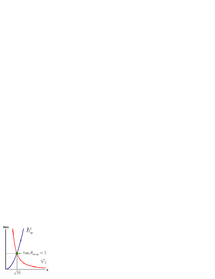
  Figure 1: Variation of the areas A$\left(x\right)$ of the spheres $\mathbb{S}_{h}^{2}$ and $\mathbb{S}_{\varphi}^{2}$ in terms of their radius $x$. In blue A_h and in red A_φ; at intersecting point $\tan\beta_{susy}=1$ and supersymmetry is restored.

• Vacuum energy $\mathcal{E}_{\min}$
  Being a non supersymmetric ground state, the energy density $\mathcal{E}_{\min}$ of the state $\left|\tilde{\Sigma}_{nsusy}\right\rangle$ is non zero and is given by

  $$\mathcal{E}_{\min}=\frac{g^{\prime 2}g^{2}}{8\left(g^{2}+g^{\prime 2}\right)}\mathrm{r}^{2}$$

  where $g$ and $g^{\prime}$ are the gauge coupling constants of the $SU_{L}\left(2\right)\times U_{Y}\left(1\right)$ gauge symmetry group.

  By using the well known standard model relations

  $$\sin\vartheta_{{}_{W}}=\frac{g^{\prime}}{\sqrt{g^{2}+g^{\prime 2}}},\qquad\cos\vartheta_{{}_{W}}=\frac{g}{\sqrt{g^{2}+g^{\prime 2}}}$$

  expressing the gauge coupling constants $g$ and $g^{\prime}$ in terms of the Weinberg angle $\vartheta_{{}_{W}}$, we then have

  $$\mathcal{E}_{\min}=\frac{\sin^{2}\left(2\vartheta_{{}_{W}}\right)}{32}\mathrm{r}^{2}$$

  and

  $$\varrho^{2}=\frac{\mathrm{r}\sin^{2}\vartheta_{{}_{W}}}{2}+\left|\mathrm{\nu}\right|\sqrt{1+\frac{\mathrm{r}^{2}\sin^{4}\vartheta_{{}_{W}}}{4\left|\mathrm{\nu}\right|^{2}}}$$ (55)

• Deviation of $\tan\beta$
  Using the relation between $\varphi_{i}$ and $\bar{h}_{i}$ that reads in present case like

  $$\varphi_{i}=\frac{\mathrm{\nu}}{\varrho^{2}}\bar{h}_{i},\qquad\varphi_{i}\bar{\varphi}^{i}=\frac{\left|\mathrm{\nu}\right|^{2}}{\varrho^{2}}$$

  one learns that the ratio of the Higgs VEVs gets modified and leads to a deviation with respect to $\tan\beta_{susy}=1$. This deviation $\tan\beta=\frac{\varrho^{2}}{\left|\mathrm{\nu}\right|}$ and is expressed in terms of the Weinberg angle of standard model of electroweak interactions like

  $$\tan\beta=\frac{\mathrm{r}\sin^{2}\vartheta_{{}_{W}}}{2\left|\mathrm{\nu}\right|}+\sqrt{1+\left(\frac{\mathrm{r}\sin^{2}\vartheta_{{}_{W}}}{2\left|\mathrm{\nu}\right|}\right)^{2}}$$ (56)

  From this formula, we also learn that the dimensionless parameter

  $$\frac{\mathrm{r}}{2\left|\mathrm{\nu}\right|}$$

  captures data on supersymmetry breaking. For a small supersymmetry breaking regime, we have $\frac{\mathrm{r}}{2\left|\mathrm{\nu}\right|}<<1$; so we can expand the above $\tan\beta$ relation; we get up to first order

  $$\tan\beta\simeq 1+\frac{\mathrm{r}\sin^{2}\vartheta_{{}_{W}}}{2\left|\mathrm{\nu}\right|}+\frac{1}{2}\left(\frac{\mathrm{r}\sin^{2}\vartheta_{{}_{W}}}{2\left|\mathrm{\nu}\right|}\right)^{2}$$ (57)

  For a large supersymmetry breaking regime corresponding to $\frac{\mathrm{r}}{\left|\mathrm{\nu}\right|}>>1$; we have

  $$\tan\beta\simeq\frac{\mathrm{r}\sin^{2}\vartheta_{{}_{W}}}{\left|\mathrm{\nu}\right|}$$ (58)

  but this limit is beyond the used approximation $\mathcal{V}_{ch}>>\mathcal{V}_{re}$.

• metric of ground state $\Sigma_{n\text{-}susy}$
  In the case $r\neq 0$, the metric of the ground state of the Higgs fields reads as

  $$ds_{\Sigma_{n-susy}}^{2}=\frac{1}{4}\left(\varrho^{2}+\frac{\left|\mathrm{\nu}\right|^{2}}{\varrho^{2}}\right)\left[d\theta^{2}+d\psi^{2}+d\phi^{2}+2\cos\theta d\psi d\phi\left.\begin{array}[]{c}\\ \end{array}\right.\right]$$ (59)

  where the angles $\theta,$ $\psi$ and $\phi$ are as in eqs(53-54) and $\varrho^{2}$ like in eq(55). We also have the useful relation

  $$\varrho^{2}+\frac{\left|\mathrm{\nu}\right|^{2}}{\varrho^{2}}=\mathrm{r}+\frac{2\left|\mathrm{\nu}\right|^{2}}{\mathrm{r}\sin^{2}\vartheta_{{}_{W}}+\sqrt{4\left|\mathrm{\nu}\right|^{2}+\mathrm{r}^{2}\sin^{4}\vartheta_{{}_{W}}}}$$ (60)

  Moreover, because of the symmetry (41), the Higgs fields can be written like
  

  $$h^{i}=\varrho\text{ }\left(\begin{array}[]{c}\cos\frac{\theta}{2}e^{i\phi}\\ \\ \sin\frac{\theta}{2}\end{array}\right)$$ (61)

  and

  $$\varphi_{i}=\frac{\mathrm{\nu}}{\varrho}\text{ }\left(\begin{array}[]{c}\cos\frac{\theta}{2}e^{-i\phi}\text{ }\\ \\ \sin\frac{\theta}{2}\end{array}\right)$$ (62)

  The previous metric becomes

  $$ds_{\Sigma_{n-susy}}^{2}=\frac{\varrho^{4}+\left|\mathrm{\nu}\right|^{2}}{4\varrho^{2}}\left[d\theta^{2}+4\left(\cos^{2}\frac{\theta}{2}\right)d\phi^{2}\right]$$

  with no dependence in $\psi$.
  From the knowledge of the electric charges of the components fields of the doublet $h^{i}=\left(h^{+},h^{0}\right)$ and the anti-doublet $\varphi_{i}=\left(\varphi^{-},\varphi^{0}\right)$, it follows that the angle $\phi$ parameterizes precisely the electromagnetic circle $\mathbb{S}_{em}^{1}$ with rotation generator $Q_{em}$ given by

  $$Q_{em}=\frac{\partial}{i\partial\phi}$$

• the electromagnetic point $P_{u_{1}^{em}}$
  If setting the angular variable $\theta$ to a constant; say $\theta=\chi$ with $d\chi=0$; the above metric reduces to the $\mathbb{S}_{em}^{1}$ metric

  $$ds_{\Sigma_{n-susy}}^{2}|_{\theta=\chi}=\left(\frac{\varrho^{4}+\left|\mathrm{\nu}\right|^{2}}{\varrho^{2}}\cos^{2}\frac{\chi}{2}\right)d\phi^{2}$$

  which vanishes precisely at the south point of the real 2-sphere

  $$\chi=\pi\text{ \ },\text{ \ }\mathop{\mathrm{m}od}\pi$$

  where lives $P_{u_{1}^{em}}$. There the Higgs fields $h^{i}$ and $\varphi_{i}$ take the values

  $$h^{i}=\varrho$$ ,

  (63)

  and have no electric charges.

3 Higgs vacua and intersecting conifolds

In this section, we develop the idea where the down Higgs superfield doublet $\left(\boldsymbol{H}_{d}\right)^{i}$ of n-MSSM is replaced by a chiral superfield anti-doublet $\left(\Phi_{i}\right)$. First, we study the group theoretical set up of the proposal, then we give its superfield formulation, and after we describe its link with intersecting conifold geometries.

3.1 Higgs doublet and anti-doublet in n-MSSM*

Here, we focus on the gauge and Higgs sectors of the next - to - MSSM and study the basic property that allows to replace the role of doublet $\left(\boldsymbol{H}_{d}\right)^{i}$ by the anti-doublet $\boldsymbol{\Phi}_{\bar{\imath}}$.
To fix the ideas, think about the chiral superfields $\left(\boldsymbol{H}_{d}\right)^{i}$ and $\boldsymbol{\Phi}_{\bar{\imath}}$ as transforming into the two fundamental representations of $SL\left(2,C\right)$ as exhibited below

     chiral superfield : $$\ \boldsymbol{H}_{d}^{i}$$

representation :

(64)

with the sub-index $\left(-\right)$ referring to the hypercharge. As described in previous section, this replacement leads to important consequences; in particular to a change into the two following:

• the sign of the $SU_{L}\left(2\right)$ gauge coupling constant $g$ in the gauge covariant derivative $\left(\mathcal{D}_{\mu}\varphi\right)_{\bar{\imath}}$ compared to $\left(\mathcal{D}_{\mu}h_{d}\right)^{i}$; and

• the equation of motion of the auxiliary fields $D^{\prime}$ and $D^{A}$; since eqs(19) and (28) differ as well by a sign.

3.1.1 Group theory basis of the proposal

To justify the replacement of the Higgs doublet $\boldsymbol{H}_{d}^{i}$ by the anti-doublet $\boldsymbol{\Phi}_{i}$, it is interesting to begin by recalling rapidly some basic tools and useful properties in the study of supersymmetric gauge theories in superspace with focus on n-MSSM.

1) Basic ingredients
First recall that, being a particular supersymmetric gauge theory, n-MSSM has 29 superfields, among which the 4 gauge supersymmetric multiplets; and 5 Higgs chiral multiplets carrying different charges under the non abelian gauge symmetry

$$U_{Y}\left(1\right)\times SU_{L}\left(2\right)$$

In superspace, these supersymmetric Higgs multiplets are described by 5 chiral superfields belonging to different representations of the gauge symmetry; these are:

• the hyperchargeless chiral iso-singlet $\boldsymbol{S}$ having no direct interactions with the gauge superfields; and,

• the two chiral superfield iso-doublets: the up-Higgs $\boldsymbol{H}_{u}$ and the down-Higgs $\boldsymbol{H}_{d}$ having opposite hypercharges; but same quantum charge under $SU_{L}\left(2\right)$.
  These two doublets couple to the $U_{Y}\left(1\right)$ gauge multiplet $\boldsymbol{V}^{\prime}$ in opposite ways; but with the same manner to the $SU_{L}\left(2\right)$ gauge multiplet $\boldsymbol{V}^{A}$.

Recall also that because of superspace chirality condition of the Higgs superfields namely

$$\mathcal{\bar{D}}_{\dot{a}}\boldsymbol{S}=0\boldsymbol{,\qquad}\mathcal{\bar{D}}_{\dot{a}}\boldsymbol{H}_{u}=0,\qquad\mathcal{\bar{D}}_{\dot{a}}\boldsymbol{H}_{d}=0$$

with $\mathcal{\bar{D}}_{\dot{a}}$ the usual superspace covariant derivative W , the gauge symmetry transformations of the Higgs chiral superfields require going beyond the unitary $U_{Y}\left(1\right)\times SU_{L}\left(2\right)$ to its complex extension

$$\mathbb{C}_{Y}^{\ast}\times SL\left(2,C\right)\text{ \ }{\Large\supset}\text{ \ }U_{Y}\left(1\right)\times SU_{L}\left(2\right)$$

containing the unitary gauge symmetry as a subgroup. This complex extension has a larger number of representations; in particular the two inequivalent $SL\left(2,C\right)$ fundamental iso-spinors namely

$$(\frac{1}{2},0)$$ and

So chiral superfields in n-MSSM can transform either in the fundamental representation $(\frac{1}{2},0)$ or in the anti-fundamental $(0,\frac{1}{2})$ one. To fix the ideas, the quantum numbers of chiral and antichiral superfields under SL$\left(2,C\right)$ may in general be as follows

chiral antichiral

$$(\frac{1}{2},0)$$ :

:

Gauge invariance of the Kahler potential $\mathcal{K}\left(\boldsymbol{\Psi},\boldsymbol{\Psi}^{\dagger}\right)$ of the superspace lagrangian density of n-MSSM is ensured by the implementation of the exponential of the gauge superfield multiplet $\boldsymbol{V}$ that transforms in the $(\frac{1}{2},\frac{1}{2})$ representation of $SL\left(2,C\right)$ subject to a hermiticity condition; and through which the two fundamental $(\frac{1}{2},0)$ and $(0,\frac{1}{2})$ couple. In superfield language, the typical gauge invariant coupling is given as usual by

$$\mathcal{K}\left(\boldsymbol{\Psi},\boldsymbol{\Psi}^{\dagger}\right)$$

where the chiral superfield matrix $\mathcal{U}$ stands for an arbitrary representation group element of $\mathbb{C}_{Y}^{\ast}\times SL\left(2,C\right)$ with the properties

$$\left(\mathcal{U}\right)^{-1}$$

From representation group theory view, the superfield’s coupling $\boldsymbol{\Psi}^{\dagger}$ $e^{-\boldsymbol{V}}$ $\boldsymbol{\Psi}$ may roughly be thought of as follows

$$Tr\left[\text{ \ }\left(\frac{1}{2},0\right)\text{ }\otimes\text{ }\left(\frac{1}{2},\frac{1}{2}\right)^{\otimes n}\text{ }\otimes\text{ }\left(0,\frac{1}{2}\right)\text{ \ }\right],\qquad n \geq 0$$

where we have used with $e^{-\boldsymbol{V}}=\sum\frac{1}{n!}\left(-\boldsymbol{V}\right)^{n}$. The correspondence between the leading complex $SL\left(2,C\right)$ representations and the unitary $SU_{L}\left(2\right)$ ones is as collected below

(71)

from which we learn that $(\frac{1}{2},\frac{1}{2})$ reduces to the sum of two $SU_{L}\left(2\right)$ representations.

2) Useful properties
We give two useful features on the relation between the representations of $SL\left(2,C\right)$ and those of $SU_{L}\left(2\right)$. These features can be also learnt from the correspondences of table (71).

• besides that it can be subject to a reality condition

  $$\boldsymbol{V}^{\dagger}=\boldsymbol{V}$$

  the complex 4- dimensional $SL\left(2,C\right)$ representation $(\frac{1}{2},\frac{1}{2})$, when reduced to $SU_{L}\left(2\right)$, has the remarkable property of containing a complex $SU_{L}\left(2\right)$ iso-singlet as exhibited here below

  $$(\frac{1}{2},\frac{1}{2})\text{ \ \ \ }\rightarrow\text{ \ \ \ }1\oplus 3$$ (72)

  This feature teaches us that complex 4 representation $(\frac{1}{2},\frac{1}{2})$ as well as its hermitian version contains an $SU_{L}\left(2\right)$ singlet; a desired feature for models building in elementary particles.

• the above reduction (72) down to $SU_{L}\left(2\right)$ representation is fact a particular one among two other cousin ones; namely

                                       $$SL\left(2,C\right)$$

  (73)

  The two first relations cannot be real; they are necessary complex. But all of the 3 relations lead to complex $SU_{L}\left(2\right)$ iso-singlets as exhibited on (73).
  

3) Higgs superfields vs $\mathbb{C}_{Y}^{\ast}\times SL\left(2,C\right)$
From the view of the complex $\mathbb{C}_{Y}^{\ast}\times SL\left(2,C\right)$ group representations, the quantum numbers of the Higgs chiral superfield doublets $\boldsymbol{H}_{u}$ and $\boldsymbol{H}_{d}$; as well as their adjoint conjugates $\boldsymbol{H}_{u}^{\dagger}$ and $\boldsymbol{H}_{d}^{\dagger}$ are as follows

(80)

where the $\pm q$ charges appearing as sub-indices of the $SL\left(2,C\right)$ representation $\left(j,j^{\prime}\right)_{\pm q}$ refer to the $\mathbb{C}_{Y}^{\ast}$ action:

$$\mathbb{C}_{Y}^{\ast}:\begin{tabular}[]{lll}$\boldsymbol{H}_{x}$&$\text{\ }\rightarrow\text{ \ }$&$e^{\Lambda_{0}\frac{Y}{2}}\boldsymbol{H}_{x}$\\ $\boldsymbol{H}_{x}^{\boldsymbol{\dagger}}$&$\text{\ }\rightarrow\text{ \ }$&$\boldsymbol{H}_{x}^{\boldsymbol{\dagger}}e^{\Lambda_{0}^{\boldsymbol{\dagger}}\frac{Y}{2}}$\end{tabular}$$

with $\Lambda_{0}$ a chiral superfield ($\mathcal{\bar{D}}_{\dot{a}}\Lambda_{0}=0$) and $\Lambda_{0}^{\boldsymbol{\dagger}}$ anti-chiral. $\mathbb{C}_{Y}^{\ast}$ is the complex extension of the $U_{Y}\left(1\right)$ hypercharge symmetry. Because of their opposite hypercharges and eq(73), we also have

(84)

showing that the composite chiral superfield

$$\boldsymbol{H}_{u}\boldsymbol{H}_{d}$$

and its monomials are good candidate for the chiral sector of supersymmetry; $\boldsymbol{H}_{u}\boldsymbol{H}_{d}$ can be coupled to the iso-singlet chiral superfield $\boldsymbol{S}$; but also to a hyperchargeless isotriplet chiral superfield $\vec{\Delta}$; see appendix

$$\boldsymbol{H}_{u}S\boldsymbol{H}_{d}$$

4) up Higgs $\boldsymbol{H}_{u}$ as a doublet and down Higgs $\boldsymbol{\Phi}$ as an anti-doublet
In our proposal, the $\boldsymbol{H}_{d}$ of n-MSSM is replaced by the anti-doublet chiral superfield $\boldsymbol{\Phi}$ with quantum numbers under $SL\left(2,C\right)$ as follows

(90)

with gauge transformations like

$$\boldsymbol{H}_{u}$$

(91)

With these quantum number assignments, the Higgs superfields $\boldsymbol{H}_{u}$ and $\boldsymbol{\Phi}$ have opposite charges under both factors of the gauge symmetry.
For the interesting case of the chiral sector of superspace lagrangian density, compatibility between chirality and $U_{Y}\left(1\right)\times SU_{L}\left(2\right)$ gauge invariance is explicitly exhibited in the following table

(98)

From this table we learn that as far as $U_{Y}\left(1\right)\times SU_{L}\left(2\right)$ gauge symmetry is concerned, the charge assignments as in (90) gives another possibility in looking for supersymmetric extensions of standard model (SM) of electroweak theory. The study of this extension is one of the objectives of the present study.

3.1.2 Gauge transformations

The supersymmetric extension of the standard model requires at least 4 Higgs supersymmetric chiral multiplets; these are given by the usual chiral superfield doublets $\boldsymbol{H}_{u}$ and $\boldsymbol{H}_{d}$. In next - to - MSSM, one has, in addition to the two above superfield doublets, the iso-singlet superfield $\boldsymbol{S}$.

In our proposal baptized as n-MSSM*, instead of $\boldsymbol{H}_{u}$ and $\boldsymbol{H}_{d}$, we have $\boldsymbol{H}_{u}$ and $\boldsymbol{\Phi}$ with gauge symmetry charges as in (90-98). Therefore, the gauge transformations of the 5 Higgs chiral superfields are as follows:

• the chiral superfields $\boldsymbol{S}$ and $\boldsymbol{H}_{u}\equiv\left(\boldsymbol{H}^{i}\right)$ are exactly as in n-MSSM. Under generic $SL\left(2,C\right)$ transformations preserving chirality, these 3 superfields transform as usual like

  $$\boldsymbol{S}$$

  (99)

  with gauge transformation

  $$\mathcal{U}_{{}_{sl_{2}}}=e^{+\Lambda_{A}T^{A}}\text{ \ \ \ },\qquad\mathcal{\bar{D}}_{\dot{a}}\text{ }\mathcal{U}_{{}_{sl_{2}}}=0$$ (100)

  and the gauge parameter $\Lambda=\Lambda_{A}T^{A}$ is a chiral superfield valued in the Lie algebra of $SU_{L}\left(2\right)$ gauge symmetry. Infinitesimally, we have

  $$\delta_{{}_{sl_{{\small 2}}}}\boldsymbol{S}$$

  (101)

• the 2 chiral superfields making $\boldsymbol{\Phi}_{i}$ behave as the components of an anti-doublet of $SL\left(2,C\right)$. By anti-doublet, we mean that under non abelian gauge transformations, the chiral superfields $\boldsymbol{\Phi}$ transform like

  $$\boldsymbol{\Phi}$$

  (102)

  with

  $$\mathcal{U}_{{}_{sl_{2}}}^{-1} = e^{-\Lambda_{A}T^{A}}\text{ \ \ \ },\qquad\mathcal{\bar{D}}_{\dot{a}}\left(\mathcal{U}_{{}_{sl_{2}}}^{-1}\right)=0$$ (103)

  standing for the inverse of $\mathcal{U}_{{}_{sl_{2}}}$. Infinitesimally

  $$\delta_{{}_{sl_{{\small 2}}}}\Phi_{i}$$

  (104)

  Notice that like in eq(99), the gauge transformation (102) preserves as well the chirality property. Notice also that the electric charges of the $\boldsymbol{H}_{u}$ and $\boldsymbol{H}_{d}$ components are as

  $$\left(\boldsymbol{H}_{u}\right)^{i} = \left(\begin{array}[]{c}H_{u}^{+}\\ H_{u}^{0}\end{array}\right)\qquad,\qquad\left(\boldsymbol{H}_{u}^{\dagger}\right)_{i}=\left(\bar{H}_{u}^{-},\bar{H}_{u}^{0}\right)$$ (107)

  $$\left(\boldsymbol{H}_{d}\right)^{i} = \left(\begin{array}[]{c}H_{d}^{0}\\ H_{d}^{-}\end{array}\right)\qquad,\qquad\left(\boldsymbol{H}_{d}^{\dagger}\right)_{i}=\left(\bar{H}_{d}^{0},\bar{H}_{d}^{+}\right)$$ (110)

  while for the anti-doublet $\boldsymbol{\Phi}$ they are given by

  $$\left(\boldsymbol{\Phi}\right)_{i}=\left(\Phi^{-},\Phi^{0}\right)\qquad,\qquad\left(\boldsymbol{\Phi}^{\dagger}\right)^{i}=\left(\begin{array}[]{c}\bar{\Phi}^{+}\\ \bar{\Phi}^{0}\end{array}\right)$$ (111)

The opposite choice of the quantum numbers for $\boldsymbol{\Phi}$, with respect to the standard $\boldsymbol{H}_{d}$ of n-MSSM, affects the sign of the $SU_{L}\left(2\right)$ gauge coupling constants $\boldsymbol{\Phi}_{i}$ and $\boldsymbol{\bar{\Phi}}^{i}$ as shown on the following Kahler superfield potentials

$$\mathcal{K}\left(\boldsymbol{H}_{u},\boldsymbol{H}_{u}^{\dagger}\right)$$

(112)

with $\boldsymbol{V}_{su_{2}}$ the hermitian $SU\left(2\right)$ gauge superfields. Explicitly, by expanding $e^{\pm g\boldsymbol{V}_{su_{2}}}$, we have for the first order in the gauge coupling constant $g$ the following tri-superfield couplings

$$-g\text{ }\bar{H}_{i}\times\left(\boldsymbol{V}_{su_{2}}\right)_{k}^{i}\times H^{k}$$

(113)

Using the chiral superfield doublet $H^{i}$ and the chiral anti-doublet $\Phi_{i}$, one can build the iso-scalar

$$\Phi_{i}H^{i}\text{ \ \ }\rightarrow\text{ \ \ }\Phi_{i}^{\prime}H^{i\prime}=\Phi_{i}H^{i}$$ (114)

that preserves chirality and has no hypercharge.
In addition to above features, the exotic gauge transformation (102) has been also motivated by looking for a link between supersymmetry on ground state of Higgs fields and intersecting complex 3D conifold singularities. More details are given below.

3.2 Link with conifold geometry

We start by recalling that in the study of complex 3D conifold geometries; one distinguishes two remarkable kinds of conifolds: resolved and deformed X1 -XF . These geometries are in one to one correspondence with the Kahler and chiral sectors of a particular class of supersymmetric gauge theories, such as the Higgs sector of n-MSSM* we are interested in this study. Generally, by using 4 complex coordinates, the singular version of these complex threefolds are respectively defined the following hypersurfaces

Kahler : $$\left|\boldsymbol{z}_{1}\right|^{2}+\left|\boldsymbol{z}_{2}\right|^{2}-\left|\boldsymbol{z}_{3}\right|^{2}-\left|\boldsymbol{z}_{4}\right|^{2}$$

Chiral :

(115)

In our analysis, the 4 complex variables $\boldsymbol{z}_{I}$ are the same as the $\boldsymbol{w}_{I}$’s and should thought of as given by the leading scalar fields $\left(h^{i}\right)$ and $\left(\varphi_{i}\right)$ of the chiral superfield doublet $\left(H_{u}^{i}\right)$ and the chiral anti-doublet $\left(\Phi_{i}\right)$.

3.2.1 Auxiliary field eqs of motion and conifold

In n-MSSM*, there are $5=1+2+2$ complex auxiliary fields type $F$; and $4=1+3$ hermitian auxiliary fields type $D$. These fields, which scales as mass², carry different $U_{Y}\left(1\right)\times SU_{L}\left(2\right)$ charges and are denoted in our proposal respectively as exhibited on following table

superfields : $$\boldsymbol{S}$$

bosonic fields :

fermionic fields :

auxiliary fields :

quantum charges :

(116)

It happens that the equations of motion of the two hyperchargeless iso-singlets auxiliary fields $F_{S}$ and $D^{\prime}$ have much to do with the equations (115) of the conifold singularities. Indeed, by using component Higgs fields on ground state ($h^{i}$ and $\varphi_{i}$ constant fields), we will show that the equation of motion of the hermitian $D^{\prime}$ and the complex $F_{S}$ can brought to the following forms

$$\bar{h}_{i}h^{i}-\varphi_{i}\bar{\varphi}^{i}=\mathrm{r}$$ (117)

and

$$\varphi_{i}h^{i}=\mathrm{\nu}$$ (118)

The complex number $\mathrm{\nu}$ and the real $\mathrm{r}$ are Fayet Iliopoulos coupling constants appearing in (29); and respectively interpreted as complex and Kahler deformations of conifold singularity.
In next section, we show that the general form of the equations of motion of the full set of auxiliary fields of n-MSSM are given the vanishing condition of the following relations

$$\bar{F}_{S}$$

(119)

and

$$\bar{F}_{i}$$

(120)

For $S=0$, eqs(119) reduce exactly to (117-118).

3.2.2 Solutions of auxiliary field eqs: Anticipation

The general solution of the auxiliary fields equations of motion depends on the complex parameter $\mathrm{\nu}$ and the real $\mathrm{r}$. In the case $\mathrm{r}=0$ and $\mathrm{\nu}$ an arbitrary complex number, the field equations $F^{i}=G_{i}=0$ are trivially solved by $S=0$ and one is left with the following

$$\varphi_{i}h^{i}$$

(121)

We will show later on that the solution of the two first relations are given by, see also eqs(236) for details,

$$h^{i}$$

(122)

with

$$\mathrm{f}^{i}$$ ,

(123)

We find that the iso-triplet equation $D^{A}=0$ is also exactly solved by (123); thanks to the replacement of the doublet $\boldsymbol{H}_{d}$ by the anti-doublet $\boldsymbol{\Phi}$.
These Higgs configurations parameterize a real 2-sphere $\mathbb{S}^{2}=SU\left(2\right)/U\left(1\right)$, preserve supersymmetry and leads to the VEVs ratio

$$\tan\beta_{susy}=1$$ (124)

We find as well that by switching on the hermitian FI coupling constant $\mathrm{r}\neq 0$, supersymmetry gets broken; and one ends with the following deviation of the VEVs ratio

$$\tan\beta$$

(125)

where $g$ and $g^{\prime}$ are the gauge coupling constants of $SU_{L}\left(2\right)\times U_{Y}\left(1\right)$ symmetry. For

$$\xi=\frac{g^{\prime 2}\mathrm{r}}{2\left(g^{2}+g^{\prime 2}\right)\sqrt{\mathrm{\nu\bar{\nu}}}}=\frac{\mathrm{r}\sin^{2}\vartheta_{{}_{W}}}{2\left|\mathrm{\nu}\right|}<<1$$

we have

$$\tan\beta\simeq 1+\xi+\frac{1}{2}\xi^{2}$$

To distinguish the slightly modified n-MSSM* we are interested in here from the usual next - to - MSSM, we shall refer to it below as the conifold model; its content in superfields and the interacting dynamics of its Higgs multiplets are described with some useful details in next section.

4 n-MSSM^∗ as another extension of SM

n-MSSM^∗ is a 4D supersymmetric field model given by n-MSSM; but with the doublet $\boldsymbol{H}_{d}$ replaced by the anti-doublet $\boldsymbol{\Phi}$; it has two phases characterized by the Fayet-Iliopoulous coupling constant $\left(\mathrm{r},\mathrm{\nu}\right)$ as shown on fig 2: $\left(i\right)$ a supersymmetric phase given by $r=0$ but an arbitrary complex parameter $\nu$ as in (121); and $\left(ii\right)$ a non supersymmetric phase associated with the switching on of the hermitian $r\neq 0$. A comment on explicit breaking of supersymmetry will be given in section 7.

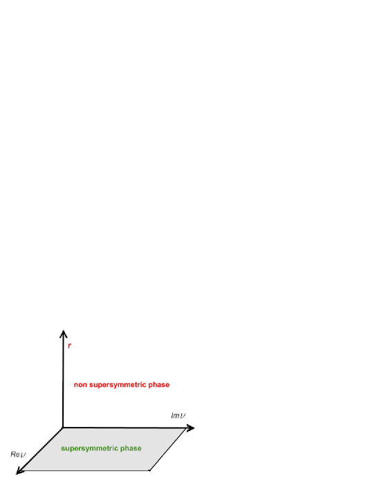
Figure 2: phases of Higgs ground state: $\left(i\right)$ $r=0$ supersymmetric phase; and $\left(ii\right)$ $r\neq 0$ the non supersymmetric one.

4.1 Superfield content and lagrangian density

We first describe the underlying quantum numbers of the superfield’s content of n-MSSM* conifold model; then we study the structure of the gauge invariant superspace lagrangian density.

4.1.1 Superfield spectrum

By ignoring lepton’s and quark’s sectors of n-MSSM*, as they are not directly involved in the determination of the Higgs ground state $\left|\Sigma_{higgs}\right\rangle$, the superfield content of the conifold model may be then restricted to 9 supersymmetric multiplets described by 9 superfields, 4 hermitian and 5 chiral; these are:

• the $U_{Y}\left(1\right)\times SU_{L}\left(2\right)$ gauge multiplets
  They are given by the usual 4 hermitian superfields $\boldsymbol{V}_{u_{1}}\left(x,\theta,\bar{\theta}\right)$ and $\boldsymbol{V}_{su_{2}}\left(x,\theta,\bar{\theta}\right)$ valued in the Lie algebra of the $U_{Y}\left(1\right)\times SU_{L}\left(2\right)$ gauge symmetry

  $$\boldsymbol{V}_{u_{1}}$$

  (126)

  with $\frac{Y}{2}$ the hermitian generator of the $U_{Y}\left(1\right)$ and $T^{A}$ the 3 generators of $SU_{L}\left(2\right)$. The $\boldsymbol{V}^{\prime}$ has no hypercharge and behaves as an iso-singlet under $SU_{L}\left(2\right)$. The $\boldsymbol{V}_{A}$’s form an iso-triplet and have no hypercharge as well.
  The $\theta$-expansion of these superfields are as usual; for the example of $V_{0}\left(x,\theta,\bar{\theta}\right)$ solving the reality condition $V_{0}^{\dagger}=V_{0}$ reads as in general like W

  $$V_{0}$$

  (127)

  where, the extra fields $\upsilon$, $\varsigma_{a}$ and $C$ are pure gauge degrees of freedom. Obviously $B_{\mu}$ is the vector gauge field, $\lambda_{a}^{\prime}$ the gaugino and $D^{\prime}$ the auxiliary field.
  A similar expansion can be written down for the three $\boldsymbol{V}_{A}$’s; their bosonic gauge fields are denoted by $W_{\mu}^{A}$ and the 3 auxiliary field ones as $D_{A}$.

• 5 chiral superfields
  They are given by the chiral superfield singlet $\boldsymbol{S}$; the chiral superfield doublet $\boldsymbol{H}^{i}$ and the anti-doublet $\boldsymbol{\Phi}_{i}$ with quantum numbers under $U_{Y}\left(1\right)\times SU_{L}\left(2\right)$ as follows

  chiral superfields $$\ \ {\small SU}_{{\small L}}{\small(2)\times U}_{{\small Y}}{\small(1)}$$

  (128)

  
  

  The iso-singlet $\boldsymbol{S}$ captures the extension of the Higgs sector of the minimal supersymmetric standard model, MSSM; it plays an important role in solving the auxiliary field equations of motion $F^{i}=0$ and $G_{i}=0$.      
  Notice also that $\boldsymbol{H}^{i}$ and $\boldsymbol{\Phi}_{i}$ have opposite quantum number under $U_{Y}\left(1\right)\times SU_{L}\left(2\right)$; this is as well an important feature in deriving non trivial solutions for the auxiliary field’s equations of motion.
  The $\theta$- expansions of these chiral superfields are given by

  $$\boldsymbol{H}^{i}\left(y,\theta\right)$$

  (129)

  with $y^{\mu}=x^{\mu}+i\theta\sigma^{\mu}\bar{\theta}$, and $\tilde{h}^{i},$ $\tilde{\varphi}_{\bar{\imath}}$, $\tilde{S}$ designating the fermionic superpartners. For antichiral superfields, we have $\bar{y}^{\mu}=x^{\mu}-i\theta\sigma^{\mu}\bar{\theta}$.
  The $U_{Y}\left(1\right)$ hypercharges of these superfields are same as in n-MSSM*; while the charges of $\boldsymbol{H}^{i}$ and $\boldsymbol{\Phi}_{i}$ under $SU_{L}\left(2\right)$ are opposite; and are as in eqs(99-102). Explicitly, we have

  $$\boldsymbol{H}^{i}$$ ,

  ,

  (130)

  with

  $$\mathcal{U} = \ e^{+g\Lambda_{A}T^{A}}\qquad,\qquad\ \ \mathcal{U}^{-1}=\ e^{-g\Lambda_{A}T^{A}}$$

  $$\mathcal{U}^{\dagger} = \ \ e^{+g\Lambda_{A}^{\dagger}T^{A}}\qquad,\qquad\mathcal{U}^{\dagger-1}=\ \ e^{-g\Lambda_{A}^{\dagger}T^{A}}$$ (131)

  where the 3 gauge super-parameters $\Lambda_{A}$ are chiral superfields and $\Lambda_{A}^{\dagger}$ the corresponding antichiral ones.
  From eqs(131), we learn that one may go from the gauge matrix $\mathcal{U}$ to its inverse $\mathcal{U}^{-1}$ and vice versa just by performing the sign change

  $$gT^{A}\quad\rightarrow\quad\left(-g\right)T^{A}$$ (132)

4.1.2 Lagrangian density of n-MSSM*

In $\mathcal{N}=1$ superspace, the lagrangian density describing supersymmetric interacting dynamics of the gauge and Higgs superfields of the conifold model (n-MSSM* ) is given by

$$\boldsymbol{L}_{conif}=\boldsymbol{L}_{gauge}+\boldsymbol{L}_{higgs}$$ (133)

The pure gauge term $\boldsymbol{L}_{gauge}$ is as usual

$$\boldsymbol{L}_{gauge}$$

(134)

and the gauge covariant term $\boldsymbol{L}_{higgs}$ describing the Higgs sector coupled to gauge multiplets reads as follows

$$\boldsymbol{L}_{higgs}$$

(135)

with

$$\left(\frac{1}{e^{-g\boldsymbol{V-g}^{\prime}\boldsymbol{V}^{\prime}}}\right) \equiv e^{+g\boldsymbol{V+g}^{\prime}\boldsymbol{V}^{\prime}}$$ (136)

where $g^{\prime}$, $g$ are the $U_{Y}\left(1\right)\times SU_{L}\left(2\right)$ gauge coupling constants and where the complex $\lambda$ and $\kappa$ are coupling constants of tri-superfield’s in the chiral superpotential.

In above expression, we have also added two kinds of Fayet-Iliopoulos (FI) terms, one with a real $\mathrm{r}$ coupling parameter and the other with complex $\mathrm{\nu}$ one; the scaled convention $\frac{g^{\prime}}{2}\mathrm{r}$ and $\lambda\mathrm{\bar{\nu}}$ are for later use. The existence of the 3 FI couplings $r,$ $\nu,$ $\bar{\nu}$ is because of a hidden $\mathcal{N}=2$ supersymmetry property of the superfield spectrum. The superfields $\boldsymbol{S}$ and $\boldsymbol{V}_{0}$ combine indeed into a $\mathcal{N}=2$ supersymmetric $U_{Y}\left(1\right)$ gauge multiplet which is known to have 3 FI coupling constants.

Notice that the lagrangian density $\boldsymbol{L}_{higgs}$ is manifestly invariant under the gauge symmetry transformations. For gauge changes under the non abelian factor, the chiral superfields $\boldsymbol{H}^{i}$ and $\boldsymbol{\Phi}_{i}$ transform as in (130) and the gauge superfields like

$$e^{-g\boldsymbol{V}}\text{ \ \ } \rightarrow \text{ \ \ }\left(\mathcal{U}^{{\small-1}}\right)^{\dagger}\times\left(e^{-g\boldsymbol{V}}\right)\times\left(\mathcal{U}^{{\small-1}}\right)$$

$$e^{+g\boldsymbol{V}}\text{ \ \ } \rightarrow \text{ \ \ }\mathcal{U}\times e^{+g\boldsymbol{V}}\times\left(\mathcal{U}^{\dagger}\right)$$

with $\mathcal{U}$ and $\mathcal{U}^{-1}$ as in eqs(131) and $e^{-g\boldsymbol{V}}e^{+g\boldsymbol{V}}=I$ due to $\left[\boldsymbol{V},\boldsymbol{V}\right]=0$. Explicitly, these superfield transformations read as

$$\left(e^{-g\boldsymbol{V}}\right)_{j}^{i}\text{ \ \ } \rightarrow \text{ \ \ }\left(\mathcal{U}^{{\small-1}}\right)_{k}^{\dagger i}\left(e^{-g\boldsymbol{V}}\right)_{l}^{k}\left(\mathcal{U}^{{\small-1}}\right)_{j}^{l}$$

$$\left(e^{+g\boldsymbol{V}}\right)_{j}^{i}\text{ \ \ } \rightarrow \text{ \ \ }\mathcal{U}_{k}^{i}\left(e^{+g\boldsymbol{V}}\right)_{l}^{k}\left(\mathcal{U}^{\dagger}\right)_{j}^{l}$$

with lower indices denoting matrix columns and upper ones the rows.

Used notations: illustrating examples
To fix the idea on the used notations, we illustrate the above matrix products by considering a useful example. First take the $2\times 2$ matrices $\mathcal{U}$ and its inverse $\mathcal{U}^{{\small-1}}$ with respective complex entries $\left(\mathcal{U}\right)_{\bar{k}}^{l}$ and $\left(\mathcal{U}^{{\small-1}}\right)_{l}^{\bar{k}}$ like

$$\mathcal{U}=\left(\begin{array}[]{cc}a&b\\ c&d\end{array}\right),\quad\mathcal{U}^{{\small-1}}=\left(\begin{array}[]{cc}d&-b\\ -c&a\end{array}\right)\text{, \ \ }ad-bc=1$$ (139)

from which we learn

$$\left(\begin{array}[]{cc}d&-b\\ -c&a\end{array}\right)^{T}=\left(\begin{array}[]{cc}0&-1\\ 1&0\end{array}\right)\left(\begin{array}[]{cc}a&b\\ c&d\end{array}\right)\left(\begin{array}[]{cc}0&1\\ -1&0\end{array}\right)$$ (140)

showing that $\left(\mathcal{U}^{{\small-1}}\right)^{T}$ and $\mathcal{U}$ are related by $\varepsilon_{ij}$ and its transpose. This feature can be also obtained by using the expression of the determinant of the $\mathcal{U}$ matrix namely $\left(\mathcal{U}_{1}^{1}\right)\left(\mathcal{U}_{2}^{2}\right)$ $-$ $\left(\mathcal{U}_{1}^{2}\right)\left(\mathcal{U}_{2}^{1}\right)$ $=$ $1$ that reads by help of the $\varepsilon$- antisymmetric tensors like

$$\varepsilon_{ij}\left(\mathcal{U}_{k}^{i}\right)\left(\mathcal{U}_{l}^{j}\right)=\varepsilon_{kl}$$ (141)

or equivalently as $\varepsilon^{mk}\mathcal{U}_{k}^{i}\varepsilon_{ij}\mathcal{U}_{l}^{j}=\delta_{l}^{m}$. From these relations, one deduces the link between $\mathcal{U}^{-1}$ and $\mathcal{U}$ which is nothing but eq(140),

$$\left(\mathcal{U}^{-1}\right)_{j}^{m}=\varepsilon^{mk}\text{ }\mathcal{U}_{k}^{i}\text{ }\varepsilon_{ij}\quad,\quad\varepsilon_{km}\left(\mathcal{U}^{-1}\right)_{j}^{m}=\mathcal{U}_{k}^{i}\varepsilon_{ij}$$ (142)

These relations can be as well derived by equating the gauge transformation of both sides of the equality $\boldsymbol{\Phi}_{i}\boldsymbol{H}^{i}=\varepsilon_{il}\boldsymbol{\Phi}^{l}\boldsymbol{H}^{i}$; we obtain

$$\boldsymbol{\Phi}_{j}\left(\mathcal{U}^{-1}\right)_{i}^{j}\left(\mathcal{U}_{k}^{i}\right)\boldsymbol{H}^{k}=\varepsilon_{il}\left(\mathcal{U}_{k}^{i}\right)\left(\mathcal{U}_{m}^{l}\right)\varepsilon^{mj}\Phi_{j}\boldsymbol{H}^{k}$$

leading to (141-142).

n-MSSM and conifold model       
Compared to usual expression in n-MSSM, the superspace lagrangian density (135) of the conifold model n-MSSM* has some special features; in particular the two following ones.

• up-Higgs free super-propagators $\left\langle\boldsymbol{H}_{i}^{\dagger}\boldsymbol{H}^{j}\right\rangle$ are same as those in n-MSSM; but $\left\langle\boldsymbol{\Phi}_{i}\boldsymbol{\Phi^{j\dagger}}\right\rangle$ come with a minus sign compared to $\left\langle\boldsymbol{H}_{di}^{\dagger}\boldsymbol{H}_{d}^{j}\right\rangle$; this feature is due to the $SU\left(2\right)$ representation group property

  $$\boldsymbol{\Phi}_{i}\boldsymbol{\Phi^{i\dagger}=}-\boldsymbol{\Phi_{i}^{\dagger}\Phi}^{i}$$

• by expanding the exponentials in (135), the hermitian tri-superfield’s couplings involving a gauge superfield are given by,

  $$-g\left(\boldsymbol{T}_{A}\right)_{j}^{i}\boldsymbol{V}^{A}\boldsymbol{H}_{i}^{\dagger}\boldsymbol{H}^{j}$$ ,

  ,

  (143)

  these interactions intervene in the structure of the equations of motion of the auxiliary fields D. As explicitly exhibited, the vertices with Higgs superfield doublet $\boldsymbol{H}^{i}$ involve the gauge coupling constants $\left(-g\right)$ and $\left(-g^{\prime}\right)$ while those with anti-doublet $\boldsymbol{\Phi}_{\boldsymbol{i}}$ involves $\left(+g\right)$ and $\left(+g^{\prime}\right)$.

Recall that in n-MSSM, the analogue of eqs(143) are directly read from the Kahler part of the gauge covariant superspace density namely

$$\mathop{\displaystyle\int}d^{4}\theta\boldsymbol{H}_{u}^{\dagger}\left[e^{-g\boldsymbol{V}_{A}T^{A}\boldsymbol{-g}^{\prime}\boldsymbol{V}_{0}\frac{Y}{2}}\right]\boldsymbol{H}_{u}+\mathop{\displaystyle\int}d^{4}\theta\boldsymbol{H}_{d}^{\dagger}\left[e^{-g\boldsymbol{V}_{A}T^{A}\boldsymbol{-g}^{\prime}\boldsymbol{V}_{0}\frac{Y}{2}}\right]\boldsymbol{H}_{d}$$ (144)

By expansion of the exponentials, one obtains the tri-superfield’s interactions; these are:

• the tri-superfield’s interactions involving the $U_{Y}\left(1\right)$ gauge superfield $\boldsymbol{V_{0}}$,

  $$\boldsymbol{-}\frac{\boldsymbol{g}\prime}{2}\boldsymbol{H}_{u}^{\dagger}\boldsymbol{V_{0}H}_{u}$$

  $$\boldsymbol{+}\frac{\boldsymbol{g}\prime}{2}\boldsymbol{H}_{d}^{\dagger}\boldsymbol{V_{0}H}_{d}$$ (145)

  which are as in (143). Because of the opposite hypercharges, they come also in a pair with opposite sign; and

• the tri-superfield’s interactions involving the $SU_{L}\left(2\right)$ gauge superfields $\boldsymbol{V_{A}}$

  $$\boldsymbol{-}g\boldsymbol{V_{A}H}_{u}^{\dagger}T^{A}\boldsymbol{H}_{u}$$

  $$\boldsymbol{-gV_{A}H}_{d}^{\dagger}T^{A}\boldsymbol{H}_{d}$$ (146)

  have the same sign of the $SU_{L}\left(2\right)$ gauge coupling constant g contrary to (143).

4.2 Supersymmetric scalar potential

First, we give the component field lagrangian; then we study the scalar potential of the conifold model.

4.2.1 Component field lagrangian density

The integration of the superspace lagrangian density (133-135) with respect to the Grassmann variables $\theta$ and $\bar{\theta}$ gives the following component field expression

$$\boldsymbol{L} = -\frac{1}{4}B_{\mu\nu}^{A}B_{A}^{\mu\nu}-\frac{1}{4}W_{\mu\nu}^{A}W_{A}^{\mu\nu}\text{ \ }+$$

$$\left[\left(\nabla_{\mu}h\right)^{i}\right]^{\dagger}\left(\nabla_{\mu}h\right)^{i}+\left(\mathcal{D}_{\mu}\varphi\right)_{i}\left[\left(\mathcal{D}_{\mu}\varphi\right)_{i}\right]^{\dagger}-\mathcal{V}_{scalar}$$

where, for simplicity, we have dropped out the fermionic contributions.
The operators $\nabla_{\mu}$ and $\mathcal{D}_{\mu}$ are $U_{Y}\left(1\right)\times SU_{L}\left(2\right)$ gauge covariant derivatives; they are not completely independent as they are associated with two representations of same gauge symmetry. The use of different notations $\nabla_{\mu}$ and $\mathcal{D}_{\mu}$ is to exhibit the opposite signs of the gauge coupling constants of the two Higgs doublets with the $W_{\mu}^{A}$ bosons seen that the doublet $h^{i}$ and anti-doublet $\varphi_{i}$ have opposite quantum numbers under $SU_{L}\left(2\right)$ as well. Thus, we have

$$\left(\nabla_{\mu}h\right)^{i}$$

(148)

showing that one may go from $\left(\nabla_{\mu}h\right)^{i}$ to $\left(\mathcal{D}_{\mu}\varphi\right)_{i}$ and vice versa by interchanging $h^{i}$ and anti-doublet $\varphi_{i}$ ( implicitly $g^{\prime}$ $\leftrightarrow$ $-g^{\prime}$ ); but also changing the sign of the $SU_{L}\left(2\right)$ gauge coupling constants

$$g\text{ \ \ }\leftrightarrow\text{ }-g$$ (149)

The tensors $B_{\mu\nu}^{A}$, $W_{\mu\nu}^{A}$ are respectively the gauge field strengths of the $SU_{L}\left(2\right)$ and $U_{Y}\left(1\right)$ gauge bosons; they are as follows

$$W_{\mu\nu}^{A}$$

(150)

with $f_{BC}^{A}$ the structure constants of $SU_{L}\left(2\right)$; and the three $2\times 2$ matrices $\tau_{A}$ the usual Pauli matrices whose entries are represented, in our convention, like

$$\left(\tau^{1}\right)_{i}^{j}=\left(\begin{array}[]{cc}0&1\\ 1&0\end{array}\right)$$ ,

(151)

The coupling of $W_{\mu}^{A}$ bosons to the Higgs field’s current $J_{A}^{\mu}$ can be written as

$$-gW_{\mu}^{A}J_{A}^{\mu}=-gW_{\mu}^{A}\left(J_{A\left(h\right)}^{\mu}-J_{A\left(\varphi\right)}^{\mu}\right)$$ (152)

with $J_{A\left(h\right)}^{\mu}$ and $J_{A\left(\varphi\right)}^{\mu}$ given by

$$J_{A\left(h\right)}^{\mu}$$

(153)

Notice that the above gauge covariant derivatives can be put into the condensed form

$$\nabla_{\mu}\boldsymbol{h}$$

(154)

with

$$\Upsilon_{\mu}=\frac{g^{\prime}}{2}B_{\mu}+gW_{\mu}^{A}\frac{\tau_{A}}{2}$$ (155)

By using the expressions of the Pauli matrices, we explicitly have

$$\Upsilon_{\mu}$$

(156)

with

$$\cos\vartheta_{{}_{W}}=\frac{g}{\sqrt{g^{2}+g^{\prime 2}}},\qquad\sin\vartheta_{{}_{W}}=\frac{g^{\prime}}{\sqrt{g^{2}+g^{\prime 2}}}$$

We also have for the quadratic terms in the vector gauge fields and the Higgs fields

$$L_{m}=\bar{h}_{i}\left(\Upsilon_{\mu}\Upsilon^{\mu}\right)_{j}^{i}h^{j}+\varphi_{i}\left(\Upsilon_{\mu}\Upsilon^{\mu}\right)_{j}^{i}\bar{\varphi}^{j}$$ (157)

where

$$\Upsilon_{\mu}\Upsilon^{\mu}=\frac{g^{2}}{4}\Theta,\qquad\Theta_{i}^{j}=\left(\begin{array}[]{cc}\Theta_{1}^{1}&\Theta_{1}^{2}\\ \Theta_{2}^{1}&\Theta_{2}^{2}\end{array}\right)$$ (158)

with

$$\Theta_{2}^{2}=2W^{+\mu}W_{\mu}^{-}+\frac{1}{\cos^{2}\vartheta_{{}_{W}}}Z^{\mu}Z_{\mu}$$ (159)

and analogous relations for the others $\Theta$’s.

Anticipation: Masses of the gauge particles
To see how the conifold geometry of the ground state is involved in the masses of the gauge particles, let us compute the masses of the $W_{\mu}^{\pm}$ and $Z_{\mu}$ by using results presented in the summary given in previous section and which will be derived later on.
Using the expression (53-54) giving the values of the Higgs fields $h^{i}$ and $\varphi_{i}$ in the ground state namely

$$h^{i}$$

(160)

with

$$\varrho^{2}+\frac{\left|\mathrm{\nu}\right|^{2}}{\varrho^{2}}=\mathrm{r}+\frac{2\left|\mathrm{\nu}\right|^{2}}{\mathrm{r}\sin^{2}\vartheta_{{}_{W}}+\sqrt{4\left|\mathrm{\nu}\right|^{2}+\mathrm{r}^{2}\sin^{4}\vartheta_{{}_{W}}}}$$ (161)

then eq(157) takes then the form

$$L_{m}=\frac{g^{2}}{4}\left(\varrho^{2}+\frac{\left|\mathrm{\nu}\right|^{2}}{\varrho^{2}}\right)\text{ }\bar{f}_{i}\Theta_{j}^{i}f^{j}$$

For the case where the angles are set to $\mathrm{\theta}=\pi$ and $\psi=\phi,$ the relations (160) reduce to

$$h^{i}$$ ,

and the $U_{Y}\left(1\right)\times SU_{L}\left(2\right)$ gauge symmetry is broken down to $U_{em}\left(1\right)$. The masses of the gauge bosons are then read from the following relation

$$L_{m}=\frac{g^{2}}{2}\left(\varrho^{2}+\frac{\left|\mathrm{\nu}\right|^{2}}{\varrho^{2}}\right)\left(W^{+\mu}W_{\mu}^{-}+\frac{1}{2\cos^{2}\vartheta_{{}_{W}}}Z^{\mu}Z_{\mu}\right)$$

from which we read the masses of the gauge fields

$$M_{W_{\mu}^{\pm}}=g\sqrt{\frac{\varrho^{4}+\left|\mathrm{\nu}\right|^{2}}{2\varrho^{2}}},\qquad M_{Z_{\mu}}=\frac{M_{W_{\mu}^{\pm}}}{\cos^{2}\vartheta_{{}_{W}}},\qquad M_{A_{\mu}}=0$$

These masses, which should be thought of as the ones given by the standard model namely

$$M_{W} = 80.385\pm 0.015GeV/c$$

$$M_{Z} = 91.1876\pm 0.0021GeV/c$$

are proportional to the square root of $\varrho^{2}+\frac{\left|\mathrm{\nu}\right|^{2}}{\varrho^{2}}$ and so are, modulo the used assumption, related to the Kahler r and complex $\mathrm{\nu}$ parameters of the intersecting conifold geometries as given by eq(161).

4.2.2 Scalar potential

Like in the usual case of next- to - MSSM, the full scalar potential $\mathcal{V}_{higgs}$ of the Higgs field of the n-MSSM^∗ with $\boldsymbol{H}_{d}$ replaced by the anti-doublet $\Phi$ ( conifold model in our terminology) is given by

$$\mathcal{V}_{higgs}=\mathcal{V}_{susy}+\mathcal{V}_{exl}$$

with $\mathcal{V}_{susy}$ the supersymmetric component

$$\mathcal{V}_{susy}=\mathcal{V}_{ch}+\mathcal{V}_{re}$$

and $\mathcal{V}_{exl}$ the explicit supersymmetry breaking term.

1) supersymmetric contributions

a) case of doublet $\boldsymbol{H}_{u}$ and anti-doublet $\Phi$
In the conifold model n-MSSM^∗ with supersymmetric lagrangian density (135), the supersymmetric scalar potential reads like

$$\mathcal{V}_{susy}^{conifold}$$

(162)

with the auxiliary fields $F$ and $D$ related to the Higgs fields as follows

$$\bar{F}_{S}$$

(163)

For later use, notice that the equation of the auxiliary field $D^{A}$ can be also expressed into a symmetric manner like

$$D^{A}=\frac{g}{4}\left(\varepsilon\tau^{A}\right)_{ij}\left[\bar{h}^{(i}h^{j)}-\varphi^{(i}\bar{\varphi}^{j)}\right]$$

Eqs(163) capture basic data on the physical properties of the Higgs fields $S$, $h^{i}$ and $\varphi_{i}$ in the ground state. Their vanishing condition involve:

• 14 hermitian coupled relations:

  • 5 of them complex holomorphic eqs given by for the auxiliary fields F,

  • 4 hermitian ones for the auxiliary fields D;

• 9 coupling constant moduli

  • 3 complex constants  namely $\lambda,$ $\kappa,$ $\nu$

  • 3 real ones$\ g,$ $g^{\prime},$ $r$

The determination of the exact solutions of eqs(163) is of a major importance; this allows to get more insight into the explicit expression of the Higgs VEVs

$$\left\langle S\right\rangle,\qquad\left\langle h^{i}\right\rangle,\qquad\left\langle\varphi_{i}\right\rangle$$

and the relations between them.

b) comparison with n-MSSM eqs
In n-MSSM based on the usual two Higgs superfield doublets $\boldsymbol{H}_{u}$ and $\boldsymbol{H}_{d}$, the scalar potential reads as

$$\mathcal{V}_{susy}^{n-mssm}$$

(164)

with

$$\left(\bar{F}_{S}\right)_{n-mssm}$$

(165)

The field equation of $D^{A}$ of eq(163) and the one of $\left(D^{A}\right)_{n-mssm}$ differ from the sign in front of the terms $\varphi^{(i}\bar{\varphi}^{j)}$ and $\bar{h}_{d}^{(i}h_{d}^{j)}$; this is due to the quantum charge property

The vanishing conditions $D^{A}=0$ and the $\left(D^{A}\right)_{{\small n}\text{-}{\small MSSM}}=0$ lead to different solutions; and therefore to different supersymmetric ground states. The same conclusion is valid for the corresponding scalar potentials and their extrema.

2) explicit supersymmetry breaking contribution

In dealing with the Higgs potential in n-MSSM and in the n-MSSM^∗ conifold version using the antidoublet $\varphi_{i}$, one extends the supersymmetric $\mathcal{V}_{susy}$ by an extra term $\mathcal{V}_{exl}$ breaking explicitly supersymmetry

$$\mathcal{V}_{higgs}=\mathcal{V}_{susy}+\mathcal{V}_{exl}$$ (167)

This term is required by low energy phenomenology. In the case of the conifold model we are interested in here, the term $\mathcal{V}_{exl}$ reads like

$$\mathcal{V}_{exl}$$

The adjunction of this term to $\mathcal{V}_{susy}$ modifies the shape of the Higgs potential which is no longer a positive function as schematized in fig 3 . Generally, it has a remarkable region with negative values.

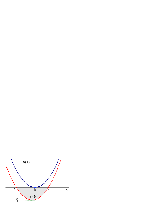
Figure 3: In red, a typical non supersymmetric potential imagined as $\frac{1}{2}\left(x-a\right)\left(x-c\right)+V_{0}$; describing a deformation of the supersymmetric shape with $a\neq c$ and $V_{0}$ induced by $\mathcal{V}_{expl}.$ For the particular case $a=c=b$ and $V_{0}=0$ (blue) one recovers supersymmetry. In terms of Higgs fields, the potential is of course quartic; it has the usual shape; say with "3 extrema": 2 minima and a local maximum.

Notice that the above $\mathcal{V}_{exl}$ can be put into the following form depending linearly in the auxiliary fields $D^{\prime}$ and $\bar{F}$ like

$$\mathcal{V}_{exl}$$

(168)

where $\Delta^{\prime}$ is as in eq(320).
In the remainder of this study, we proceed follows:

• switch off $\mathcal{V}_{exl}$ and study the ground state phases:
  the exact supersymmetric phase will be studied in section 5; and the broken supersymmetric one in section 6,

• switch on $\mathcal{V}_{exl}$ and explore the modification of the obtained results; this is studied in section 7.

5 Supersymmetric phase

In quantum supersymmetric gauge theories, the energy of the supersymmetric ground state vanishes $\mathcal{E}_{\min}^{susy}=0$; a remarkable property manifested at the level of the component field lagrangian by the positivity of the scalar potential $\mathcal{V}_{susy}$ which reads in our case like

$$\mathcal{V}_{susy}$$

(169)

This hermitian function involves various kinds of field representations namely iso-singlets $F_{S}$ and $D^{\prime}$, iso-doublets $F^{i}$, $\bar{G}^{i}$ and corresponding anti-doublets $\bar{F}_{i},$ $G_{i}$ as well as the iso-triplet $D_{A}$.

5.1 Exact supersymmetry

On supersymmetric ground state $\left|\Sigma_{susy}\right\rangle$ of the conifold model (n-MSSM with the anti-doublet $\boldsymbol{\Phi}$ instead of $\boldsymbol{H}_{d}$), described by the superspace lagrangian density (134-135), the scalar potential of the Higgs fields vanishes

$$\left.\mathcal{V}_{susy}\right|_{\Sigma_{susy}}=\mathcal{V}\left(S,\bar{S},h,\bar{h},\varphi,\bar{\varphi}\right)=0$$ (170)

This equation should be thought of as

$$\sum_{I}\mathcal{V}_{I}=0$$ (171)

a sum of several constraint equations given by $\mathcal{V}_{I}=0$; and capturing data on the allowed values of the VEVs of the Higgs fields $S,$ $h_{i},$ $\varphi_{i}$ that preserve supersymmetry.
Below, we study the set of solutions of these equations and determine the explicit expressions of these VEVs.

5.1.1 Supersymmetric ground state

The set $\Sigma_{susy}$ of the Higgs field moduli $S,$ $h_{i},$ $\varphi_{i}$, solving the vanishing condition $\mathcal{V}_{susy}=0,$ defines the exact supersymmetric phase of the model. For a geometric interpretation, we will refer to this set as

$$\Sigma_{susy}=\left\{\left.\begin{array}[]{c}\\ \end{array}\right.\left(S,h_{i},\varphi_{i}\right)\in\mathbb{C}^{5}\text{ \mbox{$|$} \ }\mathcal{V}_{susy}=0\text{ }\left.\begin{array}[]{c}\\ \end{array}\right.\text{ }\right\}$$ (172)

and, in connection with this manifold, we also need other spaces and parameterizations; in particular the real 3-spheres $\mathbb{S}_{h}^{3}$ and $\mathbb{S}_{\varphi}^{3}$ respectively parameterized by the Higgs moduli $h^{i}$ and $\varphi_{i}$ as follows

$$\mathbb{S}_{h}^{3}$$

(173)

To deal with these spheres, we need moreover the harmonic field coordinates $\mathrm{\bar{f}}_{i}$ and $\mathrm{f}^{i}$ given by eq(123); see also sub-section 5.1.3. Other related quantities are needed as well; they will be introduced at the appropriate time.

From a geometric view, the space $\Sigma_{susy}$ can be imagined as a hypersurface contained in the real 10 dimension space $\mathbb{R}^{10}$ parameterized by the 10 real degrees of freedom captured by the 5 complex Higgs fields

$$\Sigma_{susy}\text{ \ }\mathbf{\subset}\text{ \ }\mathbb{R}^{10}\sim\mathbb{C}^{5}$$ (174)

Because of the algebraic structure of the scalar potential, which is given by the sum of positive quantities, the condition $\mathcal{V}_{susy}=0$ requires then the vanishing of all auxiliary fields of eq(169).
Moreover, seen that the auxiliary fields are of two kinds: $\left(i\right)$ type $F$- complex auxiliary fields coming from chiral multiplets; and $\left(ii\right)$ type $D$ -hermitian auxiliary following from the hermitian gauge multiplets; it is useful to split these constraint relations into complex holomorphic constraint eqs and hermitian ones as follows:

$\mathbf{\alpha})$ complex

$$\bar{F}_{i} = \bar{G}^{i}=0$$

$$\bar{F}_{S} = 0$$ (175)

$\mathbf{\beta})$ hermitian

$$D^{\prime} = 0$$

$$D^{A} = 0$$ (176)

This splitting teaches us that the set $\Sigma_{susy}$, defined by eq(172), is therefore given by the intersection of two hypersurfaces $\mathfrak{C}_{\mathrm{\nu}}$ and $\mathfrak{R}_{\mathrm{r}}$ as follows

$$\Sigma_{susy}\text{ \ }=\text{ \ }\mathfrak{C}_{\mathrm{\nu}}\text{ \ }\mathop{\displaystyle\bigcap}\text{\ \ }\mathfrak{R}_{\mathrm{r}}$$ (177)

with

$$\mathfrak{C}_{\mathrm{\nu}}=\left\{\left.\begin{array}[]{c}\\ \end{array}\right.\left(S,h^{i},\varphi_{i}\right)\in\mathbb{C}^{5}\text{ }\mathbf{|}\text{ \ }\bar{F}_{i}=0,\text{ }\bar{G}^{i}=0,\text{ }\bar{F}_{S}=0\text{ }\left.\begin{array}[]{c}\\ \end{array}\right.\text{ }\right\}$$ (178)

and

$$\mathfrak{R}_{\mathrm{r}} = \left\{\left.\begin{array}[]{c}\\ \end{array}\right.\left(S,\bar{S},h^{i},\bar{h}_{i},\varphi_{i},\bar{\varphi}^{i}\right)\in\mathbb{R}^{10}\text{ \mbox{$|$} \ }D^{\prime}=0,\text{ }D^{A}=0\text{ }\left.\begin{array}[]{c}\\ \end{array}\right.\text{ }\right\}$$ (181)

Using the field equations of motion of the auxiliary fields (163), we then get the explicit expression of the constraint relations among the Higgs fields $S,$ $h^{i}$ and $\varphi_{i}$; they are given by the 5 algebraic complex holomorphic relations

$$\mathfrak{C}_{\mathrm{\nu}}$$

(182)

and the 4 hermitian ones

$$\mathfrak{R}_{\mathrm{r}}$$

(183)

Clearly, these are strong constraint relations as there are much more equations, [5 complex (182) plus 4 real (183)], than the number of variables ( 5 complex field moduli).

To derive the solutions of these eqs, we shall distinguish two cases depending on the value of the hermitian FI coupling constant: $\left(i\right)$ $r=0$ and $\left(ii\right)$ $r\neq 0.$

• case $r=0:$ exact supersymmetric phase.
  We will show that in this phase the supersymmetric ground state is completely characterized by the absolute value $\left|\mathrm{\nu}\right|$ of the complex parameter $\mathrm{\nu}$ of the deformed conifold geometry.
  Denoting the VEVs of the two Higgs fields $h^{i}$ and $\varphi_{i}$

  $$\upsilon_{h}^{0}$$      ,

  (184)

  we have

  $$\upsilon_{h}^{0}$$      ,

  and so

  $$\frac{\upsilon_{h}^{{\small 0}}}{\upsilon_{\varphi}^{{\small 0}}}\equiv\tan\beta_{susy}=1$$ (185)

  The supersymmetric phase of the Higgs ground state requires therefore $\beta_{susy}=\frac{\pi}{4}$.

• case $r\neq 0:$ broken supersymmetric phase.
  In this case, the values $\upsilon_{h}$ and $\upsilon_{\varphi}$ of the Higgs VEVs are no longer equal; and, in addition to $\left|\mathrm{\nu}\right|$, they depend as well on the hermitian FI coupling constant r and on the gauge coupling constants $g$ and $g^{\prime}$

  $$\upsilon_{h}$$

  (186)

  with explicit expression as in eqs(3.92).
  Because of this deviation induced by the Kahler parameter r, the supersymmetric value of $\tan\beta_{susy}$ gets modified into $\tan\beta$ given by eq(56); and which reads in the limit of small r as follows

  $$\tan\beta\simeq 1+\frac{g^{\prime 2}}{2\left(g^{2}+g^{\prime 2}\right)}\frac{\mathrm{r}}{\left|\mathrm{\nu}\right|}$$ (187)

  In this view, the second term proportional to $\frac{\mathrm{r}}{\left|\mathrm{\nu}\right|}$ in above relation captures a breaking of supersymmetry effect. In what follows, we give the explicit details.

5.1.2 Switching off FI coupling constant r

Setting the FI coupling constant parameter r to zero; but keeping the complex $\mathrm{\nu}$ arbitrary, the supersymmetric constraint relations become

$$\text{\ }\left\{\begin{tabular}[]{lll}$\lambda S\varphi_{i}$&$=$&$0$\\ $\lambda Sh^{i}$&$=$&$0$\\ $\kappa S^{2}+\lambda\left(\varphi_{i}h^{i}-\mathrm{\nu}\right)$&$=$&$0$\end{tabular}\right.$$ (188)

and

$$\left\{\begin{tabular}[]{lll}$\bar{h}_{i}h^{i}-\varphi_{i}\bar{\varphi}^{i}$&$=$&$0$\\ &&\\ $\left(\tau^{A}\right)_{j}^{i}\left(\bar{h}_{i}h^{j}-\varphi_{i}\bar{\varphi}^{j}\right)$&$=$&$0$\end{tabular}\right.$$ (189)

To derive the solutions of these constraint eqs, we proceed in 3 steps as follows:
First we solve the complex holomorphic eqs(188); these solutions give the structure of the set $\mathfrak{C}_{\mathrm{\nu}}$.
Then we require to the obtained solutions; i.e ($\varphi_{i},$ $h^{i}\in\mathfrak{C}_{\mathrm{\nu}}$), to satisfy also the iso-singlet constraint $D^{\prime}=0$ given by the first eq of (189).
These solutions, that belong to a subspace of $\mathfrak{C}_{\mathrm{\nu}}$, are required to satisfy as well the iso-triplet constraint $D^{A}=0$ given by the second eq of (189).

1) solving the complex eq(188)
A non trivial set of solutions of the complex holomorphic constraints is obtained into two stages: first by solving the vanishing conditions of the auxiliary field doublets $\bar{F}_{i}=0$ and $\bar{G}^{i}=0$ ensured by setting to zero the complex iso-singlet

$$S=0$$ (190)

Then putting this value back into the third complex holomorphic constraint between the two complex doublets $h^{i}$ and $\varphi_{i}$; one ends with

$$\varphi_{i}h^{i}=\mathrm{\nu}$$ (191)

But this relation is a well known equation; as it is precisely the defining equation of the complex deformed conifold singularity of the cotangent bundle of the real 3-sphere,

$$T^{\ast}S^{3}$$ (192)

Explicitly, by setting $\varphi_{i}=\left(\varphi_{1},\varphi_{2}\right)$ and $h^{i}=\left(h^{1},h^{2}\right)$, which by lowering the indices using $\varepsilon^{ij}$ tensor reads also as $h^{i}=\left(h_{2},-h_{1}\right)$, we have

$$\varphi_{1}h_{2}-\varphi_{2}h_{1}=\mathrm{\nu}$$ (193)

Notice also that eq(191) is invariant under the $U_{Y}\left(1\right)\times SU_{L}\left(2\right)$ gauge symmetry; this is a remarkable feature that is helpful for working out exact explicit solutions of this equation.

For a physical interpretation; but also for geometric view, it is interesting to use the following real 4D space equivalences

$$\mathbb{C}^{2}\text{ \ }\sim\text{ \ }\mathbb{R}^{4}\text{ \ }\sim\text{ \ }\mathbb{R}^{+}\times\mathbb{S}_{h}^{3}$$ (194)

where $\mathbb{R}_{+}$ is the positive half line and $\mathbb{S}_{h}^{3}$ is the real 3-sphere parameterized by the complex $h^{i}$ and $\bar{h}_{i}$. Its radius is related to the Higgs field moduli like

$$\varrho_{{}_{h}}=\sqrt{\sum_{i=1,2}\bar{h}_{i}h^{i}}=\sqrt{\left|\bar{h}_{1}\right|^{2}+\left|\bar{h}_{2}\right|^{2}}=\sqrt{\left|h_{u}^{0}\right|^{2}+h_{u}^{+}\bar{h}_{u}^{-}}$$ (195)

it exhibits explicitly the conifold singularity at the origin of the complex 2 space; as well as the residual $U_{em}\left(1\right)$ symmetry of the Higgs fields.

By help of the $U_{Y}\left(1\right)\times SU_{L}\left(2\right)$ gauge symmetry of eq(191), one can use the harmonic coordinate field variables $\left(f^{i},\bar{f}_{i}\right)$ of the real unit 3-sphere

$$\mathbb{S}^{3}\sim SU\left(2\right)$$

obeying $\bar{f}_{i}f^{i}=1$, to decompose the field moduli $h^{i}\equiv h^{+i}$ and $\varphi_{i}\equiv\varphi_{i}^{-}$ as

$$h^{+i} = \chi^{0}f^{+i}-\chi^{++}\bar{f}^{-i}$$

$$\bar{h}_{i}^{-} = \chi^{--}f_{i}^{+}+\bar{\chi}^{0}\bar{f}_{i}^{-}$$ (196)

and

$$\varphi_{i}^{-}$$

(197)

The explicit expressions of the harmonic field variables $\left(f^{+i},\bar{f}_{i}^{-}\right)\equiv\left(f^{i},\bar{f}_{i}\right)$ and their basic features are given by eqs(214); their physical meaning will be given later by requiring $\left(\chi^{0}\right)^{\ast}=\chi^{0}$ and $\chi^{++}=0$; see eqs(204).

Notice that in the decomposition (196), the complex component fields $\chi^{0},$ $\chi^{++}$ and their complex conjugates $\bar{\chi}^{0},$ $\chi^{--}$ are related to $h^{i}$ and $\bar{h}_{i}$ like

$$\chi^{0}$$      ,

     ,

(198)

and are nothing else the usual components Higgs fields; but in the harmonic coordinate basis. Moreover, being iso-singlets under $SU_{L}\left(2\right)$, the hypercharges carried by the fields $\chi^{0},$ $\chi^{++}$ are precisely the electric charges of the residual gauge symmetry $U_{em}\left(1\right)$ generated by

$$Q_{em}=T_{L}^{3}+\frac{Y}{2}$$ (199)

Notice also that $\chi^{0},$ $\chi^{++}$ still form an isodoublet; but under a dual $\widetilde{SU}_{L}\left(2\right)$ symmetry generated by

$$D^{++}$$

(200)

This feature can be checked explicitly by using eq(198); and computing for instance

$$D^{--}\chi^{0},\qquad D^{++}\chi^{0},\qquad\left(D^{++}\right)^{2}\chi^{0}$$

we have

$$D^{--}\chi^{0}$$

(201)

this means that $\chi^{0},$ $\chi^{++}$ is indeed a doublet under $\widetilde{SU}_{L}\left(2\right)$.

The same analysis is valid for the decomposition (197); there the pair $\xi^{0},$ $\xi^{--}$ and its complex conjugates $\bar{\xi}^{0},$ $\xi^{++}$ are given by

$$\xi^{0}$$ ,

,

(202)

Here also the pair $\left(\xi^{0},\xi^{--}\right)$ and its complex conjugate $\left(\bar{\xi}^{0},\xi^{++}\right)$ form two $\widetilde{SU}_{L}\left(2\right)$ doublets; the exhibited hypercharges coincide with the usual electric ones; seen that $\xi^{0},$ $\xi^{--}$ and $\bar{\xi}^{0},$ $\xi^{++}$ behave as singlets under $SU_{L}\left(2\right)$.

$$\left[T_{{}_{L}}^{A},\xi^{0}\right]=\left[T_{{}_{L}}^{A},\xi^{--}\right]=0$$ (203)

2) Physical meaning of $f^{i}$ and $\bar{f}_{i}$
To deal with the Higgs fields in the harmonic field coordinate basis $\left\{f^{i},\text{ }\bar{f}_{i}\right\}$, we shall think about eqs(196-197) in ground state as follows

$$h^{i}$$          ,

         ,

(204)

This choice corresponds to fixing 3 of the real 4 degrees of freedom, captured by the complex moduli $\chi^{0},$ $\chi^{++}$, as given below

$$\left(\chi^{0}\right)^{\ast}=\chi^{0}$$ ,

(205)

So the quantity

$$\bar{h}_{i}h^{i}$$

(206)

With this choice, the 4 real degrees of freedom of the complex Higgs field doublets $h^{i}$ and $\bar{h}_{i}$ are then split as $1+3$ respectively described by the real $\varrho$ and

$$f^{i}=\frac{1}{\varrho}h^{i},\qquad\bar{f}_{i}=\frac{1}{\varrho}\bar{h}_{i}$$ (207)

Seen $\bar{h}_{i}h^{i}=\varrho^{2}$ is the defining equation of a real 3- sphere $\mathbb{S}_{h}^{3}$ , one learns that $\left|\varrho\right|$ is nothing but the radius of the Higgs sphere $\mathbb{S}_{h}^{3}$. With the above coordinate basis choice, we have

$$\zeta$$          ,

         ,

(208)

In the decomposition (204), the moduli $\zeta$ and $\gamma$ are complex iso-singlet variables with hypercharges (electric charges) as

$$\left[\frac{Y}{2},\gamma\right]$$           ,

           ,

(209)

We also have

$$\left[\frac{Y}{2},f^{i}\right]$$           ,

(210)

5.1.3 The harmonics $(f^{i},\bar{f}_{i})$ and solution of complex equation

We first give some details on the harmonic field variables; then we derive the solution of the complex holomorphic equations.

1) More on harmonics $(f^{i},\bar{f}_{i})$
Recall that the defining equation of the real unit 3-sphere $\mathbb{S}^{3}$ in terms of the harmonic coordinate variables $f^{i},$ $\bar{f}_{i}$ reads like Y1 -Y3

$$\sum_{i=1,2}\bar{f}_{i}f^{i}=1$$ (211)

with indices raised and lowered by the antisymmetric $\varepsilon$- tensors. Moreover, being bosonic isodoublets, they satisfy as well the identities

$$\varepsilon_{ij}f^{i}f^{j}=0,\qquad\varepsilon^{ij}\bar{f}_{i}\bar{f}_{j}=0$$ (212)

These harmonic variables $f^{i}$ and $\bar{f}_{i}$ form a pair of complex doublet/anti-doublet that are interchanged by complex conjugation; i.e

$$\bar{f}_{i}=\overline{\left(f^{i}\right)}$$ (213)

and are related to the usual real 3 angles $\left(\theta,\psi,\phi\right)$ of the sphere $\mathbb{S}^{3}$ as follows

$$f^{i}$$ ,

(214)

From this solution, we learn that the generators $T_{3,\pm}$ and $Y$ of the gauge symmetry are realized like

$$\frac{Y}{2}$$

Moreover, being complex and related by complex conjugation, it is sometimes useful to exhibit the Cartan-Weyl charge carried by these variables; this is achieved by using the following correspondence

$$f^{i}$$

(215)

with the Cartan-Weyl charge operator precisely given by the $U_{CW}\left(1\right)$ generator

$$D^{0}=f^{+i}\frac{\partial}{\partial f^{+i}}-\bar{f}^{-i}\frac{\partial}{\partial\bar{f}^{-i}}$$

of the $\widetilde{su}\left(2\right)$ algebra generated by the operators (200). Indeed, we have

$$\left[D^{0},f^{+i}\right]$$

(216)

and

$$\left[D^{++},f^{+i}\right]$$

(217)

showing that ($f^{+i},\bar{f}^{-i}$) form a doublet under $\widetilde{su}\left(2\right)$.

2) the solution of holomorphic constraint eqs
Substituting the decomposition (204) back into the complex holomorphic constraint $\varphi_{i}h^{i}=\mathrm{\nu}$ of eq(191), one ends with a relation between the iso-singlets $\varrho$ and $\zeta$; but $\gamma$ free;

γ=arbitrary C-number\left\{\begin{tabular}[]{lll}$\varrho\zeta$&$=$&$\mathrm{\nu}$\\ $\gamma$&$=$&{\small arbitrary C-number}\end{tabular}\right.

ϱζ=ν (218)

from which we learn

$$\zeta=\frac{\mathrm{\nu}}{\varrho}$$ (219)

For the case $\varrho\neq 0$ and the complex parameter $\mathrm{\nu}\rightarrow 0$, the variable $\zeta$ $\rightarrow 0$; while for the case $\zeta\neq 0$, the limit $\mathrm{\nu}\rightarrow 0$ requires the vanishing of the radius $\varrho$ of the 3-spheres $\mathbb{S}_{h}^{3}$ and so this limit is singular and describes the shrinking of $\mathbb{S}_{h}^{3}$ to the origin of $\mathbb{C}_{h}^{2}$.

In conclusion, by using the harmonic coordinates $f^{i}$ and $\bar{f}_{i}$ of the unit 3-sphere $\mathbb{S}^{3}$, the set $\mathfrak{C}_{\mathrm{\nu}}$ of solutions of the complex holomorphic constraint equations

$$\left\{\begin{tabular}[]{lll}$\lambda S\varphi_{i}$&$=$&$0$\\ $\lambda Sh^{i}$&$=$&$0$\\ $\kappa S^{2}+\lambda\left(\varphi_{i}h^{i}-\mathrm{\nu}\right)$&$=$&$0$\end{tabular}\right.$$ (220)

is given by the following complex 3D hypersurface in $\mathbb{C}^{5}$,

$$S$$

(221)

with $\gamma$ an arbitrary complex iso-singlet carrying $\left(-2\right)$ hypercharges units. The metric of this threefold in terms of the coordinates $f^{i}$ and $\gamma$ reads as

$$ds_{\mathfrak{C}_{\nu}}^{2}$$

(222)

see appendix B for details and for the expression of $ds_{\mathfrak{C}_{\nu}}^{2}$ in terms of the angles $\theta,\psi$ and $\phi$.

5.2 Solving the hermitian eqs(189)

There are two kinds of hermitian constraint equations; $\left(i\right)$ the iso-singlet constraint relation following from the equation of motion of the $U_{Y}\left(1\right)$ auxiliary field $D^{\prime}$,

$$\bar{h}_{i}h^{i}-\varphi_{i}\bar{\varphi}^{i}=0$$ (223)

and $\left(ii\right)$ the hermitian iso-triplet constraint relation coming from the equation of motion of the $SU_{L}\left(2\right)$ auxiliary field $D^{A}$ namely

$$\left(\tau^{A}\right)_{j}^{i}\left(\bar{h}_{i}h^{j}-\varphi_{i}\bar{\varphi}^{j}\right)=0$$ (224)

We shall first solve eq(223) by using the Higgs configurations (221), obtained by solving the complex holomorphic constraints. Then, we put the obtained solutions solving (223) back into (224) to get the final Higgs configurations in the supersymmetric ground state. Actually this solution constitutes one of the basic results of this paper.

5.2.1 Solving iso-singlet constraint eq(223)

Using the expressions the Higgs doublet $\varphi_{i}=\frac{\mathrm{\nu}}{\varrho}\bar{f}_{i}-\gamma f_{i}$ and its complex conjugate $\bar{\varphi}^{i}=\bar{\gamma}\bar{f}^{i}+\frac{\mathrm{\bar{\nu}}}{\varrho}f^{i}$ as well as the identities $f_{i}\bar{f}^{i}=\bar{f}_{i}f^{i}=-1$, it not difficult to check that the real number $\varphi_{i}\bar{\varphi}^{i}$ reads as

$$\varphi_{i}\bar{\varphi}^{i}=\left(\gamma\bar{\gamma}+\frac{\mathrm{\nu\bar{\nu}}}{\varrho^{2}}\right)$$ (225)

and its square root $\sqrt{\varphi_{i}\bar{\varphi}^{i}}$ may be thought of as the radius of the real 3-sphere $\mathbb{S}_{\varphi}^{3}$ embedded in $\mathbb{C}_{\varphi}^{2}\sim\mathbb{R}_{+}\times\mathbb{S}_{\varphi}^{3}$. Clearly this 3-sphere $\mathbb{S}_{\varphi}^{3}$ is fibred over the 3- sphere $\mathbb{S}_{h}^{3}$ with radius $\varrho$ introduced previously and associated with the Higgs doublet $h^{i}$. This fibration, manifested in (225) by the dependence in $\varrho$, can be seen for instance on the example where $\mathrm{\nu}$ is a fixed complex number and $\varrho\rightarrow 0$; there the sphere $\mathbb{S}_{h}^{3}$ shrinks to a point while $\mathbb{S}_{\varphi}^{3}$ expands to infinity.

Substituting the above expression of $\varphi_{i}\bar{\varphi}^{i}$ back into eq(223) and using $\bar{h}_{i}h^{i}=\varrho^{2}$, the iso-singlet constraint relation $D^{\prime}=0$ becomes

$$\varrho^{2}-\left(\gamma\bar{\gamma}+\frac{\mathrm{\nu\bar{\nu}}}{\varrho^{2}}\right)=0$$ (226)

it depends on the complex deformation parameter; and gives a constraint relation between the real $\varrho$ and the complex $\gamma$ reducing thus the dimension of the space of solutions down to 4 real dimensions (2 complex). As this equation may be also put into the form

$$\varrho^{4}-\gamma\bar{\gamma}\varrho^{2}-\mathrm{\nu\bar{\nu}}=0$$ (227)

the acceptable solution leading to $\varrho^{2}>0$ and expressing $\varrho$ in terms of $\gamma$ reads like

$$\varrho^{2}=\frac{1}{2}\left(\gamma\bar{\gamma}+\sqrt{\left(\gamma\bar{\gamma}\right)^{2}+4\left(\mathrm{\nu\bar{\nu}}\right)}\right)$$ (228)

From (226), we can also express $\gamma\bar{\gamma}$ in terms of $\varrho$; we have

$$\gamma\bar{\gamma}=\varrho^{2}-\frac{\mathrm{\nu\bar{\nu}}}{\varrho^{2}}$$ (229)

Combining the solutions eqs(221), of the complex constraint eqs, with the solution (228) of the hermitian iso-singlet constraint, we then have $S=0$ and

$$h^{i}$$

(230)

The Higgs field configurations solving the complex $F_{I}=0$ and the isosinglet $D^{\prime}=0$ are expressed in terms of $\gamma\bar{\gamma}$ and on the harmonic field variables. Moreover seen that $\gamma\bar{\gamma}$ is gauge invariant; in particular under the U${}_{Y}\left(1\right)$ hypercharge transformations, one may use this arbitrariness to fix a real degree of freedom of $\gamma$, say the phase of $\left|\gamma\right|e^{-2i\delta}$, and ends afterwards with a real 4D manifold $\mathfrak{M}_{4}$ (a complex surface ) given by

$$\mathfrak{M}_{4}=\left\{\left.\begin{array}[]{c}\\ \\ \end{array}\right.\frac{eqs(\ref{3})}{U_{Y}\left(1\right)}\right\}\subset\mathfrak{C}_{\nu}$$

and contained in turns into $\mathbb{C}^{4}$ $\sim$ $\mathbb{R}^{8}$.

5.2.2 Solving the iso-triplet eq(224)

We begin by computing the quantity $\varphi_{i}\bar{\varphi}^{j}$ as it plays a central role in the isotriplet constraint; its trace $\delta_{j}^{i}\varphi_{i}\bar{\varphi}^{j}$ is precisely given (225).
Putting the expression (221) of the Higgs fields $\varphi_{i}$ and $\bar{\varphi}^{j}$, in terms of the harmonic variables $\bar{f}_{i}$ and $f^{j}$ back into the constraint eq(224), we obtain

$$\varphi_{i}\bar{\varphi}^{j}$$

(231)

Then, using the symmetry property of the iso-triplet manifested by the feature $\left(\varepsilon\tau^{A}\right)_{ij}=\left(\varepsilon\tau^{A}\right)_{ji}$ with matrices $\left(\varepsilon\tau^{A}\right)_{ij}=\varepsilon_{ik}\left(\tau^{A}\right)_{j}^{k}$, we can put the constraint relation $D^{A}=0$ into the form

$$\left(\varepsilon\tau^{A}\right)^{ij}\left[\frac{-1}{2}\left(\varrho^{2}-\frac{\mathrm{\nu\bar{\nu}}}{\varrho^{2}}+\gamma\bar{\gamma}\right)\bar{f}_{(i}f_{j)}-\frac{\mathrm{\bar{\nu}}\gamma}{2\varrho}f_{i}f_{j}+\frac{\mathrm{\nu}\bar{\gamma}}{\varrho}\bar{f}_{i}\bar{f}_{j}\right]=0$$ (232)

whose solution requires the vanishing of the coefficients of each of the iso-triplets $\bar{f}_{(i}f_{j)},$ $f_{i}f_{j}$ and $\bar{f}_{i}\bar{f}_{j}$ namely

$$\varrho^{2}-\frac{\mathrm{\nu\bar{\nu}}}{\varrho^{2}}+\gamma\bar{\gamma}$$

(233)

Seen that the complex parameter $\mathrm{\nu}$ has been taken as an arbitrary complex number of the deformed conifold, the two last relations are solved by

$$\gamma=0$$ (234)

reducing further the dimension of the space of the Higgs VEVs down to a complex curve.
Putting $\gamma=0$ back into the first relation, we end with the following non trivial solution for $\varrho$,

$$\varrho^{4}=\mathrm{\nu\bar{\nu}}$$ (235)

and then a non trivial solution for the chargeless Higgs component of the $\varphi_{i}$ Higgs doublet.

To conclude, the set $\Sigma_{susy}$ of solutions the constraint equations for a supersymmetric ground state $\left|\Sigma_{susy}\right\rangle$ with the complex FI coupling constant $\mathrm{\nu}$ arbitrary; but the real $r=0$, reads as follows

$$S$$

(236)

These Higgs configurations parameterize a real 2-sphere $\mathbb{S}_{susy}^{2}$ with radius $\varrho_{0}=\left(\mathrm{\nu\bar{\nu}}\right)^{\frac{1}{4}}$. More precisely, the sphere $\mathbb{S}_{susy}^{2}$ may be parameterized either by $h^{i}$ or by $\varphi_{i}$. If using the complex coordinates $h^{i}=\left(\mathrm{\nu\bar{\nu}}\right)^{\frac{1}{4}}f^{i}$; the doublet $\varphi_{i}$ is nothing but

$$\varphi_{i}$$

(237)

and so one is left with the 3 real degrees of freedom captured by the harmonic field variables parameterizing a 3- sphere $\mathbb{S}_{susy}^{3}\sim SU\left(2\right)$. However, seen that the Higgs configuration are symmetric under the hypercharge symmetry

$$f^{i}\text{ \ \ }\rightarrow\text{ \ \ }f^{i\prime}\equiv f^{i}$$ (238)

the ground state reduces then to

$$\mathbb{S}_{susy}^{2}\text{ \ }\sim\text{ \ }\frac{SU\left(2\right)}{U_{Y}\left(1\right)}$$

Notice that the radius $\varrho_{0}$ of the real 2-sphere $\mathbb{S}_{susy}^{2}$ can be computed either by using the $h^{i}$ variable or the $\varphi_{i}$ one; it is given by

$$\bar{h}_{i}h^{i}$$

(239)

leading in turns to

$$\tan\beta_{susy}=1$$ (240)

Regarding the isotriplet constraint eqs; they are as well identically satisfied by the solution (236) due to the identity

$$\bar{h}_{i}h^{j}$$

(241)

For such VEVs of the complex Higgs fields; that is for Higgs fields $h^{i}$ and $\varphi_{i}$ living on $\mathbb{S}_{susy}^{2}$, supersymmetry is preserved; otherwise it is broken.

6 Broken supersymmetry and ground state energy

In previous section we have shown that for $r=0$ supersymmetry of n-MSSM with anti-doublet $\Phi_{i}$ at place of $H_{d}$ is preserved for arbitrary non zero complex parameter $\nu$. In this section, we study the spontaneous breaking of supersymmetry by switching on the hermitian FI term

$$\mathrm{r}D^{\prime}=\mathrm{r}\int d^{4}\theta\text{ }\boldsymbol{V}_{{\small u}_{{}_{{\small 1}}}}^{\prime}$$

in the lagrangian density of the conifold model (135).

6.1 Switching on hermitian FI term r

By switching on the FI coupling constant $r\neq 0$; the complex holomorphic constraint eqs following from F-terms remain the same as in the case $r=0$; namely

$$\left\{\begin{tabular}[]{lll}$\lambda S\varphi_{i}$&$=$&$0$\\ $\lambda Sh^{i}$&$=$&$0$\\ $\kappa S^{2}+\lambda\left(\varphi_{i}h^{i}-\mathrm{\nu}\right)$&$=$&$0$\end{tabular}\right.$$ (242)

while the hermitian constraint relations given by the D-terms get modified. More precisely, it is the isosinglet constraint which changes like

$$\bar{h}_{i}h^{i}-\varphi_{i}\bar{\varphi}^{i}=\mathrm{r,\qquad r}\neq 0$$ (243)

but the isotriplet remains as before

$$\left(\tau^{A}\right)_{j}^{i}\left(\bar{h}_{i}h^{j}-\varphi_{i}\bar{\varphi}^{j}\right)=0$$ (244)

Because of this Kahler deformation, the previous solution with $r=0$ is no longer valid in present case.

To deal with these deformed constraint relations, we proceed as follows:

• First, we solve the complex (242) in terms of the harmonic variables $f_{i}$ and $\bar{f}_{i}$; these calculations give the solutions of the complex holomorphic constraint relations $F_{I}=0$; they are same as in previous section; and their explicit expressions are as follows

  $$S$$

  (245)

  with $\varrho=\sqrt{\bar{h}_{i}h^{i}}$.  As in case $r=0$, these Higgs configurations depend on the deformation parameter $\mathrm{\nu}$ and on the arbitrary complex $\gamma$; they parameterize a complex 3D manifold namely a deformed conifold.

• Then, we use the above expressions (245) of the Higgs $h^{i}$ and $\varphi_{i}$ to solve the iso-singlet constraint relation (243).

• After that we check whether the obtained solutions for eq(243) are consistent or not with the solutions of the iso-triplet constraint eq(244).

6.1.1 Solving iso-singlet constraint (243)

Using the expressions (245) of the Higgs fields $h_{i}$ and $\varphi_{i}$, we have $\bar{h}_{i}h^{i}=\varrho^{2}$ and $\varphi_{i}\bar{\varphi}^{i}=\gamma\bar{\gamma}+\frac{\mathrm{\nu\bar{\nu}}}{\varrho^{2}}$; then substituting back into the iso-singlet constraint eq(243) we obtain the following equation

$$\varrho^{2}-\left(\gamma\bar{\gamma}+\frac{\mathrm{\nu\bar{\nu}}}{\varrho^{2}}\right)$$

(246)

giving a relation between the real $\varrho$, the complex $\gamma$ and the FI coupling constants $\nu$ and r. For non zero $\varrho^{2}$, the above relation can be also put into the equivalent form

$$\varrho^{4}-\left(\mathrm{r}+\gamma\bar{\gamma}\right)\varrho^{2}-\mathrm{\nu\bar{\nu}}=0$$ (247)

whose solution with positive $\varrho^{2}$ is given by

$$\varrho^{2}=\frac{1}{2}\left[\left(\mathrm{r}+\gamma\bar{\gamma}\right)+\sqrt{\left(\mathrm{r}+\gamma\bar{\gamma}\right)^{2}+4\mathrm{\nu\bar{\nu}}}\right]$$ (248)

We can also express $\gamma$ in terms of $\varrho$ and the FI parameters; we have

$$\gamma\bar{\gamma}$$

(249)

Putting (248) back into the expression (245), we obtain the explicit solution of the iso-singlet $D^{\prime}=0$ in terms of the Kahler parameter $\mathrm{r,}$ the complex deformation parameter $\nu$, the variable $\gamma$ and the harmonic field variables; it is given by $S=0$ and

$$h^{i}$$

(250)

In the limit $r=0$, one recovers the previous result, see eqs(230).
In what follows, we show that for $r\neq 0,$ the above Higgs configurations are not solutions of the iso-triplet constraint relations $D^{A}=0$.

6.1.2 Solving the isotriplet eq(244)

Using the expression

$$\left(\tau^{A}\right)_{j}^{i}\varphi_{i}\bar{\varphi}^{j}$$

(251)

the hermitian isotriplet constraint (244) gets mapped to

$$\frac{1}{2}\left(\varepsilon\tau^{A}\right)_{ij}\left[\text{ \ }\left(\varrho^{2}-\gamma\bar{\gamma}-\frac{\mathrm{\nu\bar{\nu}}}{\varrho^{2}}\right)\bar{f}^{(i}f^{j)}+\gamma\frac{\mathrm{\bar{\nu}}}{\varrho}f^{i}f^{j}-\bar{\gamma}\frac{\mathrm{\nu}}{\varrho}\bar{f}^{i}\bar{f}^{j}\text{ \ \ }\right]$$

(252)

Substituting the relation $\varrho^{2}-\frac{\mathrm{\nu\bar{\nu}}}{\varrho^{2}}-\gamma\bar{\gamma}=\mathrm{r}$, required by the iso-singlet constraint $D^{\prime}=0$, the isotriplet eq(252) can be brought to the following form

$$\left(\varepsilon\tau^{A}\right)_{ij}\left[\frac{\mathrm{r}}{2}\bar{f}^{(i}f^{j)}+\gamma\frac{\mathrm{\bar{\nu}}}{2\varrho}f^{(i}f^{j)}-\bar{\gamma}\frac{\mathrm{\nu}}{2\varrho}\bar{f}^{(i}\bar{f}^{j)}\right]=0$$ (253)

whose solution requires the vanishing of each of the coefficients $\bar{f}^{(i}f^{j)}$, $f^{(i}f^{j)}$ and $\bar{f}^{(i}\bar{f}^{j)}$ namely

$$\gamma\frac{\mathrm{\bar{\nu}}}{\varrho}$$

(254)

However, the Kahler parameter should be non zero, $r\neq 0$; and so there is no common solution for the constraint eqs $D^{\prime}=0$ and $D^{A}=0.$

To conclude, for FI coupling $\mathrm{r}\neq 0$, the auxiliary field equations of motion have then no common solution. So supersymmetry of the ground state with non zero Higgs VEVs is spontaneously broken by the switching on the FI coupling constant $\mathrm{r}$.

6.2 ground state energy density

Seen that supersymmetry of the model is spontaneously broken for $r\neq 0$, then the ground state should have a non zero positive energy. In this sub-section, we compute the amount of this energy in terms of the coupling constants of the model.
To that purpose, recall that in supersymmetric gauge theories the component scalar field potential energy density $\mathcal{V}_{scalar}$ is the sum of two kinds of positive contributions: $\left(i\right)$ a term $\mathcal{V}_{ch}=\mathcal{V}\left(F,\bar{F}\right);$ and $\left(ii\right)$ a term $\mathcal{V}_{re}=\mathcal{V}\left(D\right)$;

$$\mathcal{V}_{scalar}=\mathcal{V}_{ch}+\mathcal{V}_{re}$$ (255)

the first contribution comes from the superpotential of the chiral sector of the superspace lagrangiant density $\boldsymbol{L}$ (133-135); it reads in the case we are considering here like

$$\mathcal{V}_{ch}$$

(256)

The second contribution comes from the hermitian Kahler sector the superspace lagrangian density $\boldsymbol{L}$; it is given by

$$\mathcal{V}_{re}=\frac{1}{2}D^{\prime 2}+\frac{1}{2}D_{A}D^{A}$$ (257)

The objective is to determine, within the approximation of section 2, the expression of this potential energy density in terms of the Higgs fields $S,$ $h^{i},$ $\varphi_{i}$; and then compute its minimum.

6.2.1 Non supersymmetric ground state

We start from the superspace lagrangian density (133-135) with non zero FI coupling constants $\left(\mathrm{\nu},\mathrm{r}\right)\neq\left(0,0\right)$. Seen that Higgs field configurations in the ground state are functions of the coupling constants of the model, the energy density of the ground state is also of function of these couplings,

$$\mathcal{E}_{\min}=\mathcal{E}\left(g,g^{\prime},r,\left|\nu\right|\right)$$ (258)

with the property

$$\lim_{r\rightarrow 0}\mathcal{E}_{\min}=0$$ (259)

because for $r=0$ both $\mathcal{V}_{ch}=0$ and $\mathcal{V}_{re}=0$ and so there is no vacuum energy.
For $r\neq 0$, the Higgs VEV configurations solving the complex holomorphic constraint relations (the equations of motion of the auxiliary fields F) have indeed a non zero energy density seen that

$$\mathcal{V}_{ch}=0$$ , but

(260)

where $\mathcal{V}_{re}$ is thought of as a perturbation with respect to $\mathcal{V}_{ch}$ within the approximation described in section 2.

1) computational method
After recalling useful tools on non supersymmetric ground state; we compute the expression of its energy density $\mathcal{V}_{scalar}$ in terms of the Higgs fields. Then, we determine the expression of the Higgs VEVs

$$\left\langle S\right\rangle_{\min}$$

(261)

that minimize the ground state energy density. We end this study by computing the deviation $\tan\beta$ of the supersymmetric $\tan\beta_{0}=1$ by help of the formula

$$\tan\beta=\sqrt{\frac{\left\langle\bar{h}_{i}h^{i}\right\rangle_{\min}}{\left\langle\varphi_{i}\bar{\varphi}^{i}\right\rangle_{\min}}}$$ (262)

and determining the exact expression of $\mathcal{E}_{\min}$.

2) Energy density of non supersymmetric ground state
First recall that the complex holomorphic constraint relations given by the equations of motion of the auxiliary fields

$$F^{i}=0,\qquad G^{i}=0,\qquad F_{S}=0$$ (263)

are independent on the real FI coupling parameter r. Their solutions are also independent on r; they read as

$$S = 0$$

$$h^{i} = \varrho f^{i}\qquad,\qquad\varphi_{i}=\frac{\mathrm{\nu}}{\varrho}\bar{f}_{i}-\gamma f_{i}$$

$$\bar{h}_{i} = \varrho\bar{f}_{i}\qquad,\qquad\bar{\varphi}^{i}=\frac{\mathrm{\bar{\nu}}}{\varrho}f^{i}+\bar{\gamma}\bar{f}^{i}$$ (264)

and lead to no energy density since

$$\mathcal{V}_{ch}=0$$

Using this property of $\mathcal{V}_{ch}$, the scalar potential energy density $\mathcal{V}$ of the model reduces to the part $\mathcal{V}_{re}$ coming from Kahler sector namely

$$\mathcal{V}=\frac{1}{2}D^{\prime 2}+\frac{1}{2}D_{A}D^{A}$$ (265)

with the auxiliary D- fields as

$$D^{\prime} = \frac{g^{\prime}}{2}\left(\bar{h}_{i}h^{i}-\bar{\varphi}_{i}\varphi^{i}-\mathrm{r}\right)$$

$$D^{A} = \frac{g}{2}\left(\tau^{A}\right)_{j}^{i}D_{i}^{j}$$ (266)

$$D_{i}^{j} = \bar{h}_{i}h^{j}-\varphi_{i}\bar{\varphi}^{j}$$

where $h^{i}$ and $\varphi_{i}$ are as in eqs(264).
Substituting these relations back into (265), we find, after straightforward calculations, that the explicit field expression of the gauge invariant scalar potential energy density of the non supersymmetric ground state reads in terms of the FI coupling constants and the gauge invariant variables $\varrho^{2}$ and $\gamma\bar{\gamma}$ as follows

$$\mathcal{V} = \frac{g^{\prime 2}}{8}\mathrm{r}^{2}-\frac{g^{2}}{2}\mathrm{\bar{\nu}\nu}-\frac{2g^{\prime 2}}{8}\mathrm{r}\left(\varrho^{2}-\frac{\mathrm{\nu\bar{\nu}}}{\varrho^{2}}-\gamma\bar{\gamma}\right)+$$

$$\frac{g^{\prime 2}}{8}\left(\varrho^{2}-\frac{\mathrm{\nu\bar{\nu}}}{\varrho^{2}}-\gamma\bar{\gamma}\right)^{2}+\frac{g^{2}}{8}\left[\varrho^{2}+\frac{\mathrm{\nu\bar{\nu}}}{\varrho^{2}}+\gamma\bar{\gamma}\right]^{2}$$

This scalar energy density is a function of the hermitian gauge invariants $\varrho^{2}$ and $\gamma\bar{\gamma}$

$$\mathcal{V}=\mathcal{V}\left(\varrho^{2};\gamma\bar{\gamma}\right)$$ (268)

and depends on the 5 coupling moduli namely the 2 real gauge coupling constants $g$ and $g\prime$ and the 3 the FI couplings $r$, $\mathrm{\nu},\mathrm{\bar{\nu}}$.

Deriving eq(LABEL:V0)
Here we give the main steps of the explicit derivation of the component field expression (LABEL:V0) of the scalar potential energy density $\mathcal{V}$. First, we compute the contribution coming from the term $\frac{1}{2}D^{\prime 2}$; then we calculate the contribution of $\frac{1}{2}D_{A}D^{A}$.

• computing $\frac{1}{2}D^{\prime 2}$
  The relation between the auxiliary field $D^{\prime}$ and the Higgs fields $h^{i}$ and $\varphi_{i}$ is given by (266). Using $h^{i}\bar{h}_{i}=\varrho^{2}$, one of the two basic variables of (LABEL:V0) scaling as mass² and manifestly gauge invariant, the contribution to the energy of the non supersymmetric ground state, coming from $D^{\prime},$ reads then as

  $$\frac{1}{2}D^{\prime 2}=\frac{g^{\prime 2}}{8}\left(\varrho^{2}-\varphi_{i}\bar{\varphi}^{i}-\mathrm{r}\right)^{2}$$ (269)

  or equivalently by expanding

  $$\frac{1}{2}D^{\prime 2}$$

  (270)

  with the $\varphi_{i}\bar{\varphi}^{i}$ gauge invariant as

  $$\varphi_{i}\bar{\varphi}^{i}=\frac{\mathrm{\nu\bar{\nu}}}{\varrho^{2}}+\gamma\bar{\gamma}$$ (271)

  For later use notice that for $\gamma=0$, eq(270) reduces to

  $$\frac{1}{2}D^{\prime 2}=\frac{g^{\prime 2}}{8}\left(\varrho^{2}-\frac{\mathrm{\nu\bar{\nu}}}{\varrho^{2}}-\mathrm{r}\right)^{2}$$ (272)

  and then

  $$\frac{1}{2}\frac{\partial\left(D^{\prime 2}\right)}{\partial\varrho^{2}}=\frac{g^{\prime 2}}{4}\left(\varrho^{2}-\frac{\mathrm{\nu\bar{\nu}}}{\varrho^{2}}-\mathrm{r}\right)\left(1+\frac{\mathrm{\nu\bar{\nu}}}{\varrho^{4}}\right)$$ (273)

• computing $\frac{1}{2}D_{A}D^{A}$
  Expanding the isotriplet auxiliary field $D^{A}$ in terms of the 3 Pauli matrices $\tau^{A}$ like $D^{A}=\frac{g}{2}\left(\tau^{A}\right)_{j}^{i}D_{i}^{j}$ and using the identity

  $$\left(\tau_{A}\right)_{k}^{l}\left(\tau^{A}\right)_{j}^{i}=2\delta_{k}^{i}\delta_{j}^{l}-\delta_{j}^{i}\delta_{k}^{l}$$ (274)

  we can put the term $D_{A}D^{A}$ into the form

  $$D_{A}D^{A}=\frac{g^{2}}{4}\left[2\left(D_{i}^{j}D_{j}^{i}\right)-\left(D_{i}^{i}\right)^{2}\right]$$ (275)

  with $\left(D_{i}^{j}D_{j}^{i}\right)$ and $\left(D_{i}^{i}\right)^{2}$ as follows:

  $$2D_{i}^{j}D_{j}^{i} = 2\varrho^{4}+2\left(\bar{\varphi}_{i}\varphi^{i}\right)^{2}-4\left(\varphi_{i}h^{i}\right)\left(\bar{h}_{j}\bar{\varphi}^{j}\right)$$

  $$\left(D_{i}^{i}\right)^{2} = \varrho^{4}+\left(\bar{\varphi}_{i}\varphi^{i}\right)^{2}-2\varrho^{2}\left(\bar{\varphi}_{i}\varphi^{i}\right)$$ (276)

  where $\bar{\varphi}_{i}\varphi^{i}$ is as in eq(271), and where $\varphi_{i}h^{i}$ and $\bar{h}_{j}\bar{\varphi}^{j}$ are given by

  $$\varphi_{i}h^{i} = \mathrm{\nu}$$

  $$\bar{h}_{j}\bar{\varphi}^{j} = \mathrm{\bar{\nu}}$$ (277)

  Substituting these relations back into (275), we obtain the contribution to the scalar energy density coming from the isotriplet term; it reads as

  $$\frac{1}{2}D_{A}D^{A} = \frac{g^{2}}{8}\left(\left[\varrho^{2}+\left(\bar{\varphi}_{i}\varphi^{i}\right)\right]^{2}-4\mathrm{\bar{\nu}\nu}\right)$$

  $$= \frac{g^{2}}{8}\left[\varrho^{2}+\left(\bar{\varphi}_{i}\varphi^{i}\right)+2\left|\mathrm{\nu}\right|\right]\left[\varrho^{2}+\left(\bar{\varphi}_{i}\varphi^{i}\right)-2\left|\mathrm{\nu}\right|\right]$$

  Explicitly, we have

  $$\frac{1}{2}D_{A}D^{A}=\frac{g^{2}}{8}\left[\varrho^{2}+\frac{\mathrm{\nu\bar{\nu}}}{\varrho^{2}}+\gamma\bar{\gamma}\right]^{2}-\frac{g^{2}}{2}\mathrm{\bar{\nu}\nu}$$ (279)

  Notice that for $\gamma=0$, we have

  $$\frac{1}{2}D_{A}D^{A}=\frac{g^{2}}{8}\left[\varrho^{2}+\frac{\mathrm{\nu\bar{\nu}}}{\varrho^{2}}\right]^{2}-\frac{g^{2}}{2}\mathrm{\bar{\nu}\nu}$$ (280)

  and

  $$\frac{1}{2}\frac{\partial\left(D_{A}D^{A}\right)}{\partial\varrho^{2}}=\frac{g^{2}}{4}\left(\varrho^{2}+\frac{\mathrm{\nu\bar{\nu}}}{\varrho^{2}}\right)\left(1-\frac{\mathrm{\nu\bar{\nu}}}{\varrho^{4}}\right)$$ (281)

Combining eqs(270-279), we obtain

$$\mathcal{V}=\frac{g^{\prime 2}}{8}\left(\varrho^{2}-\frac{\mathrm{\nu\bar{\nu}}}{\varrho^{2}}-\gamma\bar{\gamma}-\mathrm{r}\right)^{2}+\frac{g^{2}}{8}\left(\varrho^{2}+\frac{\mathrm{\nu\bar{\nu}}}{\varrho^{2}}+\gamma\bar{\gamma}\right)^{2}-\frac{g^{2}}{2}\mathrm{\bar{\nu}\nu}$$ (282)

which can also rewritten as in (LABEL:V0).

6.2.2 Minimizing the scalar potential

The scalar potential $\mathcal{V}$ is function of the gauge invariant quantities $\gamma\bar{\gamma}$ and $\varrho^{2}$; its extremum is then obtained by solving the conditions

$$\frac{\partial\mathcal{V}}{\partial\bar{\gamma}} = \gamma\frac{\partial\mathcal{V}}{\partial\left(\gamma\bar{\gamma}\right)}=0$$

$$\frac{\partial\mathcal{V}}{\partial\bar{h}_{i}} = h^{i}\frac{\partial\mathcal{V}}{\partial\varrho^{2}}=0$$

The set $\Upsilon$ of solutions of these relations is then given by the intersection of two sets $\Omega_{1}$ and $\Omega_{2}$ like

$$\Upsilon=\Omega_{1}\cap\Omega_{2}$$ (284)

with

$$\Omega_{1} = \left\{\gamma=0,\text{ }\frac{\partial\mathcal{V}}{\partial\left(\gamma\bar{\gamma}\right)}\text{ arbitrary}\right\}\cup\left\{\frac{\partial\mathcal{V}}{\partial\left(\gamma\bar{\gamma}\right)}=0\right\}$$

$$\Omega_{2} = \left\{h_{i}=0,\text{ }\frac{\partial\mathcal{V}}{\partial\varrho^{2}}\text{ arbitrary}\right\}\cup\left\{\frac{\partial\mathcal{V}}{\partial\varrho^{2}}=0\right\}$$

In what follows, we determine the explicit expression of the sets $\Omega_{1}$ and $\Omega_{2}$; but to fix the ideas, we will show that the common solution of (LABEL:co) corresponds to

$$\gamma = 0$$

$$\frac{\partial\mathcal{V}}{\partial\varrho^{2}} = 0$$ (286)

and reads in terms of the coupling constants and the FI parameters as follows

$$\gamma = 0$$

$$\varrho^{2} = \frac{1}{2\left(g^{2}+g^{\prime 2}\right)}\left[g^{\prime 2}\mathrm{r}+\sqrt{g^{\prime 4}\mathrm{r}^{2}+4\left(g^{2}+g^{\prime 2}\right)^{2}\mathrm{\nu\bar{\nu}}}\right]$$

1) computing $\frac{\partial\mathcal{V}}{\partial\left(\gamma\bar{\gamma}\right)}=0$
Using the expression (LABEL:V0) of the scalar potential, we have

$$\frac{\partial\mathcal{V}^{0}}{\partial\left(\gamma\bar{\gamma}\right)} = -\frac{g^{\prime 2}}{4}\left(\varrho^{2}-\frac{\mathrm{\nu\bar{\nu}}}{\varrho^{2}}-\gamma\bar{\gamma}-\mathrm{r}\right)+\frac{g^{2}}{4}\left(\varrho^{2}+\frac{\mathrm{\nu\bar{\nu}}}{\varrho^{2}}+\gamma\bar{\gamma}\right)$$ (288)

which reads also like

$$\frac{\partial\mathcal{V}}{\partial\left(\gamma\bar{\gamma}\right)} = \frac{1}{\varrho^{2}}\left[\frac{g^{2}-g^{\prime 2}}{4}\varrho^{2}+\left(\frac{2g^{\prime 2}}{8}\mathrm{r}+\frac{g^{2}+g^{\prime 2}}{4}\gamma\bar{\gamma}\right)\varrho^{2}+\mathrm{\nu\bar{\nu}}\frac{g^{2}+g^{\prime 2}}{4}\right]$$ (289)

whose solution, for $g^{2}\neq g^{\prime 2}$, is obtained by solving

$$\varrho^{4}-\frac{g^{\prime 2}\mathrm{r}+\left(g^{2}+g^{\prime 2}\right)\gamma\bar{\gamma}}{g^{\prime 2}-g^{2}}\varrho^{2}-\mathrm{\nu\bar{\nu}}\frac{g^{2}+g^{\prime 2}}{g^{\prime 2}-g^{2}}=0$$ (290)

The solution $\left\langle\varrho^{2}\right\rangle_{{}_{{}^{\gamma}}}=\left\langle\varrho^{2}\right\rangle_{\frac{\partial\mathcal{V}}{\partial\left(\gamma\bar{\gamma}\right)}=0}$ is given by

$$\left\langle\varrho^{2}\right\rangle_{{}_{{}^{\gamma}}} = \frac{g^{\prime 2}\mathrm{r}+\left(g^{2}+g^{\prime 2}\right)\gamma\bar{\gamma}}{2\left(g^{\prime 2}-g^{2}\right)}+\frac{1}{2}\sqrt{\left(\frac{g^{\prime 2}\mathrm{r}+\left(g^{2}+g^{\prime 2}\right)\gamma\bar{\gamma}}{g^{\prime 2}-g^{2}}\right)^{2}+\frac{4\mathrm{\nu\bar{\nu}}\left(g^{2}+g^{\prime 2}\right)}{g^{\prime 2}-g^{2}}}$$

2) computing $\frac{\partial\mathcal{V}}{\partial\varrho^{2}}=0$
Doing the same thing but now with respect to the variable $\varrho^{2}$, we have, by using the expression (LABEL:V0), the following expression for $\frac{\partial\mathcal{V}}{\partial\varrho^{2}},$

$$\frac{\partial\mathcal{V}}{\partial\varrho^{2}} = +\frac{g^{\prime 2}}{4}\left[\varrho^{2}-\frac{\mathrm{\nu\bar{\nu}}}{\varrho^{2}}-\gamma\bar{\gamma}-\mathrm{r}\right]\left(1+\frac{\mathrm{\nu\bar{\nu}}}{\varrho^{4}}\right)$$ (291)

$$+\frac{g^{2}}{4}\left[\varrho^{2}+\frac{\mathrm{\nu\bar{\nu}}}{\varrho^{2}}+\gamma\bar{\gamma}\right]\left(1-\frac{\mathrm{\nu\bar{\nu}}}{\varrho^{4}}\right)$$

To get the zeros of $\frac{\partial\mathcal{V}}{\partial\varrho^{2}}$, we put the solution $\gamma=0$ solving the constraint relation $\frac{\partial\mathcal{V}}{\partial\bar{\gamma}}=0$ back into the above equation; this leads to the reduced expression

$$\frac{\partial\mathcal{V}}{\partial\varrho^{2}}|_{\gamma=0} = \left(1+\frac{\mathrm{\nu\bar{\nu}}}{\varrho^{4}}\right)\left(\frac{g^{2}+g^{\prime 2}}{4}\varrho^{2}-\frac{g^{2}+g^{\prime 2}}{4}\frac{\mathrm{\nu\bar{\nu}}}{\varrho^{2}}-\frac{g^{\prime 2}}{4}\mathrm{r}\right)$$ (292)

whose zeros are obtained by solving the vanishing condition

$$\frac{g^{2}+g^{\prime 2}}{4}\varrho^{2}-\frac{g^{2}+g^{\prime 2}}{4}\frac{\mathrm{\nu\bar{\nu}}}{\varrho^{2}}-\frac{g^{\prime 2}}{4}\mathrm{r}=0$$ (293)

Rewriting this equation like

$$\varrho^{4}-\frac{g^{\prime 2}\mathrm{r}}{g^{2}+g^{\prime 2}}\varrho^{2}-\mathrm{\nu\bar{\nu}}=0$$ (294)

it is not difficult to check that the acceptable solution is given by

$$\left\langle\varrho^{2}\right\rangle=\frac{g^{\prime 2}\mathrm{r}+\sqrt{g^{\prime 4}\mathrm{r}^{2}+4\left(g^{2}+g^{\prime 2}\right)^{2}\mathrm{\nu\bar{\nu}}}}{2\left(g^{2}+g^{\prime 2}\right)}$$ (295)

Notice that for the limit $r=0$, one has

$$\left\langle\varrho_{0}^{2}\right\rangle=\sqrt{\mathrm{\nu\bar{\nu}}}$$ (296)

which should compared with eq(235) obtained previously when the Kahler parameter r was switched off.

To conclude, the minimum of the scalar potential $\mathcal{V}=\frac{1}{2}D^{\prime 2}+\frac{1}{2}D_{A}D^{A}$ with the auxiliary fields related to the Higgs fields as follows

$$D^{\prime} = \bar{h}_{i}h^{i}-\varphi_{i}\bar{\varphi}^{i}-\mathrm{r}$$

$$D^{A} = \left(\tau^{A}\right)_{j}^{i}\left(\bar{h}_{i}h^{j}-\varphi_{i}\bar{\varphi}^{j}\right)$$ (297)

is obtained by first solving the conditions $\mathcal{V}_{ch}=0$ leading to

$$\left\{\begin{tabular}[]{lll}$\lambda S\varphi_{i}$&$=$&$0$\\ $\lambda Sh^{i}$&$=$&$0$\\ $\kappa S^{2}+\lambda\left(\varphi_{i}h^{i}-\mathrm{\nu}\right)$&$=$&$0$\end{tabular}\right.$$ (298)

ensured by taking $S=0$ and the Higgs fields $h_{i}$ and $\varphi_{i}$ as in eq(264). Putting these expressions back into $\mathcal{V}=\frac{1}{2}D^{\prime 2}+\frac{1}{2}D_{A}D^{A}$, one gets an explicit expression of the potential in terms of the Higgs doublets given by (LABEL:V0) with minimum given by the following non trivial VEVs completely characterized by the gauge coupling constants and the FI coupling parameters,

$$\left\langle h^{i}\right\rangle = \left(\frac{g^{\prime 2}\mathrm{r}+\sqrt{g^{\prime 4}\mathrm{r}^{2}+4\left(g^{2}+g^{\prime 2}\right)^{2}\mathrm{\nu\bar{\nu}}}}{2\left(g^{2}+g^{\prime 2}\right)}\right)^{\frac{1}{2}}\cdot\mathrm{f}^{i}$$

$$\left\langle\bar{h}_{i}\right\rangle = \left(\frac{g^{\prime 2}\mathrm{r}+\sqrt{g^{\prime 4}\mathrm{r}^{2}+4\left(g^{2}+g^{\prime 2}\right)^{2}\mathrm{\nu\bar{\nu}}}}{2\left(g^{2}+g^{\prime 2}\right)}\right)^{\frac{1}{2}}\cdot\mathrm{\bar{f}}_{i}$$

and

$$\varphi_{i} = \mathrm{\nu}\left(\frac{2\left(g^{2}+g^{\prime 2}\right)}{g^{\prime 2}\mathrm{r}+\sqrt{g^{\prime 4}\mathrm{r}^{2}+4\left(g^{2}+g^{\prime 2}\right)^{2}\mathrm{\nu\bar{\nu}}}}\right)^{\frac{1}{2}}\cdot\mathrm{\bar{f}}_{i}$$

$$\bar{\varphi}^{i} = \mathrm{\bar{\nu}}\left(\frac{2\left(g^{2}+g^{\prime 2}\right)}{g^{\prime 2}\mathrm{r}+\sqrt{g^{\prime 4}\mathrm{r}^{2}+4\left(g^{2}+g^{\prime 2}\right)^{2}\mathrm{\nu\bar{\nu}}}}\right)^{\frac{1}{2}}\cdot\mathrm{f}^{i}$$

From this solution, we determine the numbers

$$\left\langle\bar{h}_{i}h^{i}\right\rangle = \frac{g^{\prime 2}\mathrm{r}+\sqrt{g^{\prime 4}\mathrm{r}^{2}+4\left(g^{2}+g^{\prime 2}\right)^{2}\mathrm{\nu\bar{\nu}}}}{2\left(g^{2}+g^{\prime 2}\right)}$$

$$\left\langle\varphi_{i}\bar{\varphi}^{i}\right\rangle = \mathrm{\nu\bar{\nu}}\left(\frac{2\left(g^{2}+g^{\prime 2}\right)}{g^{\prime 2}\mathrm{r}+\sqrt{g^{\prime 4}\mathrm{r}^{2}+4\left(g^{2}+g^{\prime 2}\right)^{2}\mathrm{\nu\bar{\nu}}}}\right)$$

whose ratio reads as

$$\frac{\left\langle\bar{h}_{i}h^{i}\right\rangle}{\left\langle\varphi_{i}\bar{\varphi}^{i}\right\rangle} = \frac{1}{\mathrm{\nu\bar{\nu}}}\left(\frac{g^{\prime 2}\mathrm{r}+\sqrt{g^{\prime 4}\mathrm{r}^{2}+4\left(g^{2}+g^{\prime 2}\right)^{2}\mathrm{\nu\bar{\nu}}}}{2\left(g^{2}+g^{\prime 2}\right)}\right)^{2}$$ (302)

From this quantity, we obtain $\tan\beta$ which can be put into the form

$$\tan\beta = \frac{g^{\prime 2}\mathrm{r}}{2\left(g^{2}+g^{\prime 2}\right)\sqrt{\mathrm{\nu\bar{\nu}}}}+\sqrt{1+\left(\frac{g^{\prime 2}\mathrm{r}}{2\left(g^{2}+g^{\prime 2}\right)\sqrt{\mathrm{\nu\bar{\nu}}}}\right)^{2}}$$ (303)

Notice that for $r=0$, we have $\tan\beta$ $\rightarrow$ $\tan\beta_{susy}=1$. For non zero Kahler parameter r, this quantity is clearly different from unity. Moreover, for small values of $\frac{\mathrm{r}}{\left|\mathrm{\nu}\right|}$ such as,

$$\frac{g^{\prime 2}}{2\left(g^{2}+g^{\prime 2}\right)}\frac{\mathrm{r}}{\left|\mathrm{\nu}\right|}<<1$$ (304)

we have

$$\tan\beta \simeq 1+\frac{g^{\prime 2}\mathrm{r}}{2\left(g^{2}+g^{\prime 2}\right)\left|\mathrm{\nu}\right|}+\frac{1}{2}\left(\frac{g^{\prime 2}\mathrm{r}}{2\left(g^{2}+g^{\prime 2}\right)\left|\mathrm{\nu}\right|}\right)^{2}$$ (305)

The energy $\mathcal{E}_{\min}$ of the ground state is given by

$$\mathcal{E}_{\min} = \frac{g^{\prime 2}}{8}\left(\varrho^{2}-\frac{\mathrm{\nu\bar{\nu}}}{\varrho^{2}}-\mathrm{r}\right)^{2}+\frac{g^{2}}{8}\left(\varrho^{2}+\frac{\mathrm{\nu\bar{\nu}}}{\varrho^{2}}\right)^{2}-\frac{g^{2}}{2}\mathrm{\bar{\nu}\nu}$$ (306)

which reads also like

$$\mathcal{E}_{\min} = \frac{g^{\prime 2}}{8}\left(\varrho^{2}-\frac{\mathrm{\nu\bar{\nu}}}{\varrho^{2}}-\mathrm{r}\right)^{2}+\frac{g^{2}}{8}\left[2\varrho^{2}-\left(\varrho^{2}-\frac{\mathrm{\nu\bar{\nu}}}{\varrho^{2}}\right)\right]^{2}-\frac{g^{2}}{2}\mathrm{\bar{\nu}\nu}$$ (307)

But using the relations

$$\varrho^{2}-\frac{\mathrm{\nu\bar{\nu}}}{\varrho^{2}} = \frac{g^{\prime 2}}{g^{2}+g^{\prime 2}}\mathrm{r}$$

$$2\varrho^{2} = \frac{g^{\prime 2}\mathrm{r}+\sqrt{g^{\prime 4}\mathrm{r}^{2}+4\left(g^{2}+g^{\prime 2}\right)^{2}\mathrm{\nu\bar{\nu}}}}{\left(g^{2}+g^{\prime 2}\right)}$$

we can put $\mathcal{E}_{\min}$ into the form

$$\mathcal{E}_{\min}=\frac{g^{\prime 2}g^{2}}{8\left(g^{2}+g^{\prime 2}\right)}\mathrm{r}^{2}$$ (309)

7 Explicit supersymmetry breaking

Explicit supersymmetry breaking in n-MSSM is achieved by adding to the supersymmetric scalar potential $\mathcal{V}_{susy}$ the following extra term

$$\mathcal{V}_{exl}$$

(310)

involving 5 new coupling parameters in addition to the existing ones: 3 real masses $m_{{}_{{}_{u}}},$ $m_{{}_{d}}$, $m_{s}$; and the 2 complex $m_{ud}$ and $A_{{}_{\lambda}}$; see also and appendix A.

7.1 Explicit potential with anti-doublet $\varphi_{i}$

By replacing the doublet $h_{{}_{d}}^{i}$ by the anti-doublet $\varphi_{i}$, the above explicit potential gets mapped to

$$\mathcal{V}_{exl}$$

(311)

with the two following remarkable features.

• gauge invariant composites.
  Besides the complex singlet $S$, the potential $\mathcal{V}_{exl}$ involves four other gauge invariant composites of the Higgs field doublets and anti-doublets; these are:

  hermitian : $$\bar{h}_{i}h^{i}$$ ,

  complex : ,

  (312)

  Using the harmonic field coordinate basis,

  $$h^{i}$$

  (313)

  with $\xi$ and $\eta$ two complex variables; and the relations

  $$\bar{h}_{i}h^{i}$$

  (314)

  the above potential $\mathcal{V}_{exl}$ reads as

  $$\mathcal{V}_{exl}$$

  (315)

• $\mathcal{V}_{exl}$ in terms of auxiliary fields
  The above gauge invariant bilinear (312) appear as well into the equations of motion of the auxiliary fields $F_{S}$ and $D^{\prime}$

  $$\bar{F}$$

  (316)

  For the particular case $m_{{}_{u}}^{2}$ $=-m_{\varphi}^{2}=m^{2}$, the term $m_{{}_{u}}^{2}$ $\left(\bar{h}_{i}h^{i}-\varphi_{i}\bar{\varphi}^{i}\right)$ coincides exactly with $\frac{m^{2}}{g^{\prime}}D^{\prime}$, and the explicit breaking potential is expressed in terms of the auxiliary fields like

  $$\mathcal{V}_{exl}$$

  (317)

  In the general case where $m_{{}_{u}}^{2}$ and $m_{\varphi}^{2}$ are arbitrary real numbers, one needs to introduce the following exotic auxiliary field

  $$\Delta^{\prime}$$

  (318)

  This fields may be thought of as related to an extra $U^{\prime\prime}\left(1\right)$ gauge symmetry with gauge coupling constant $g^{\prime\prime}$ and under which the Higgs fields $h^{i}$ and $\varphi_{i}$ have the same charge. By inverting the relations (316-317), we obtain

  $$\varphi_{i}h^{i}$$

  (319)

  and ends with the following expression

  $$\mathcal{V}_{exl}$$

  (320)

  depending linearly on the auxiliary fields $\Delta^{\prime},$ $D^{\prime}$ and $\bar{F}$; and having an indefinite sign responsible for the negative region in fig 3.

7.2 Potential $\mathcal{V}_{exl}$ in superspace

Here, we consider a particular $\mathcal{V}_{exl}$ resulting from giving special non zero VEVs to the two hyperchargeless iso-singlet superfields $\boldsymbol{S}_{u_{1}}$ and $\boldsymbol{V}_{u_{1}}$. By special non zero VEVs we mean those superfield vacuum expectation values that break supersymmetry explicitly in the sense they depend on the Grassmann variables as follows

$$\left\langle\boldsymbol{V}_{u_{1}}\right\rangle$$

(321)

with $m_{x}$ and $A_{\kappa}$ constant coefficients as above.
Substituting these expressions back into the lagrangian density $\boldsymbol{L}_{higgs}$ given by eq(135); but with $\boldsymbol{V}^{\prime}=\boldsymbol{V}_{0}\frac{Y}{2}$ and $\boldsymbol{S}$ thought of as describing supersymmetric fluctuations like

$$\boldsymbol{V}_{0}$$

(322)

with $\left\langle\boldsymbol{V}_{u_{1}}\right\rangle$ and $\left\langle\boldsymbol{S}_{u_{1}}\right\rangle$ as in eqs(321), we obtain

$$\mathcal{L}_{higgs}$$

(323)

Using the relations

$$e^{\boldsymbol{-g}^{\prime}\left(\boldsymbol{V}^{\prime}+\theta^{2}\bar{\theta}^{2}m_{x}^{2}\right)}$$

(324)

and integrating with respect to the Grassmann variables $\theta$ and $\bar{\theta}$, we get

$$\mathcal{L}_{higgs}$$

(325)

with $L_{0}=\left|A_{\kappa}\right|^{2}-\nu A_{\kappa}-\bar{\nu}\bar{A}_{\kappa}$ a constant term scaling as mass⁴ and interpreted in terms of vacuum energy density; it will be dropped out in what follows.
The field doublets $h^{i\prime}$ and $\varphi_{i}^{\prime}$ of the second line of eq(325) are related to the usual doublets $h^{i}$ and $\varphi_{i}$ like

$$h^{i\prime} \equiv e^{\boldsymbol{-}\frac{\boldsymbol{g}^{\prime}}{4}\boldsymbol{\upsilon}_{0}}\left(e^{-\frac{g}{4}\boldsymbol{\upsilon}_{A}\tau^{A}}\right)_{j}^{i}h^{j}$$

$$\varphi_{i}^{\prime} \equiv \varphi_{j}\left(e^{+\frac{g}{4}\boldsymbol{\upsilon}_{A}\tau^{A}}\right)_{i}^{j}e^{\boldsymbol{+}\frac{\boldsymbol{g}^{\prime}}{4}\boldsymbol{\upsilon}_{0}}$$ (326)

with $\boldsymbol{\upsilon}_{A}$ and $\boldsymbol{\upsilon}_{0}$ standing respectively for the leading component fields of the $\theta$- expansion of the $SU_{L}\left(2\right)$ and the $U_{Y}\left(1\right)$ gauge multiplets $\boldsymbol{V}_{A}$ and $\boldsymbol{V}_{0}$. They read as

$$\boldsymbol{\upsilon}_{A} = \boldsymbol{V}_{A}\boldsymbol{|}_{\theta=\bar{\theta}=0}$$

$$\boldsymbol{\upsilon}_{0} = \left(\boldsymbol{V}_{0}\right)\boldsymbol{|}_{\theta=\bar{\theta}=0}$$ (327)

and are pure gauge degrees of freedom. However, because of $\mathbb{C}_{Y}^{\ast}\times SL\left(2,C\right)$ property, the doublet $h^{i\prime}$ and anti-doublet $\varphi_{i}^{\prime}$ can be identified with $h^{i}$ and $\varphi_{i}$ respectively due to the residual symmetry transformations leaving in the coset space,

$$\frac{\mathbb{C}_{Y}^{\ast}\times SL\left(2,C\right)}{U_{Y}\left(1\right)\times SU_{L}\left(2\right)}$$

Notice also that in the Wess- Zumino gauge vector multiplets, the quantities $\boldsymbol{\upsilon}_{A}$ and $\boldsymbol{\upsilon}_{0}$ appearing in (326) are simply set to zero.

7.3 Energy of the ground state

In this subsection, we use the potential approximation

$$\mathcal{V}=\mathcal{V}_{ch}+\mathcal{V}_{pert}$$

with

$$\mathcal{V}_{pert}=\left(\frac{1}{2}D^{\prime 2}+\frac{1}{2}D_{A}D^{A}\right)+\mathcal{V}_{exl}$$

to study the effect induced by the $\mathcal{V}_{exl}$ potential on the predictions of previous sections. In this approximation, the minimum of $\mathcal{V}_{ch}$ is given by the Higgs fields configuration

$$\left\{\begin{tabular}[]{lll}$\lambda S\varphi_{i}$&$=$&$0$\\ $\lambda Sh^{i}$&$=$&$0$\\ $\kappa S^{2}+\lambda\left(\varphi_{i}h^{i}-\mathrm{\nu}\right)$&$=$&$0$\end{tabular}\right.$$ (328)

solved as

$$S = 0$$

$$\varphi_{i} = \frac{\mathrm{\nu}}{\varrho^{2}}\bar{h}_{i}-\frac{\gamma}{\varrho}h_{i}$$ (329)

$$h^{i} = \varrho f^{i}$$

Notice that there is no contribution of the Higgs iso-singlet Higgs field $S$ nor in $\varphi_{i}h^{i}$; the main role of $S$ is to fix of the shape of the Higgs VEVS as

$$\varphi_{i}h^{i}=\mathrm{\nu}$$ (330)

Then, because of $\varphi_{i}h^{i}=\mathrm{\nu}$ and $S=0$, the contribution of $\mathcal{V}_{exl}$ coming from the chiral sector drops out; no the complex term plus its complex conjugate in $\mathcal{V}_{exl}$; so the explicit potential reduces to

$$\mathcal{V}_{exl}=\mathcal{V}_{0}+g^{\prime}m_{x}^{2}\left(\bar{h}_{i}h^{i}-\varphi_{i}\bar{\varphi}^{i}\right)$$

with $\mathcal{V}_{0}=cte$. Therefore, the resulting Higgs potential reads, up to a constant, like

$$\mathcal{V}=\frac{1}{2}D^{\prime 2}+\frac{1}{2}D_{A}D^{A}+g^{\prime}m_{x}^{2}\left(\bar{h}_{i}h^{i}-\varphi_{i}\bar{\varphi}^{i}\right)$$ (331)

with an indefinite sign and a field variation completely originating from the Kahler sector of supersymmetry. The last feature can be explicitly exhibited by expressing $\left(\bar{h}_{i}h^{i}-\varphi_{i}\bar{\varphi}^{i}\right)$ in term of the auxiliary field $D^{\prime}$. Using

$$D^{\prime}$$

(332)

we have

$$\left(\bar{h}_{i}h^{i}-\varphi_{i}\bar{\varphi}^{i}\right)=\frac{2}{g^{\prime}}\left(D^{\prime}+2\mathrm{r}\right)$$

and then

$$\mathcal{V}=\frac{1}{2}D_{A}D^{A}+\frac{1}{2}D^{\prime 2}+\frac{2m_{x}^{2}}{g^{\prime}}\left(D^{\prime}+\mathrm{r}\right)$$ (333)

In addition to the usual quadratic $\frac{1}{2}D^{\prime 2}$, the Higgs potential $\mathcal{V}$ has also a linear dependence on $D^{\prime}$. Moreover, seen that this potential may be also rewritten as

$$\mathcal{V}=\frac{1}{2}D_{A}D^{A}+\frac{1}{2}\left(D^{\prime}+\frac{m_{x}^{2}}{g^{\prime}}\right)^{2}+\frac{2m_{x}^{2}}{g^{\prime}}\left(\mathrm{r}-\frac{m_{x}^{2}}{4g^{\prime}}\right)$$ (334)

or more explicitly like

$$\mathcal{V}=\frac{g^{\prime 2}}{8}\left(\varrho^{2}-\frac{\mathrm{\nu\bar{\nu}}}{\varrho^{2}}-\gamma\bar{\gamma}-\mathrm{r}+\frac{m_{x}^{2}}{g^{\prime}}\right)^{2}+\frac{g^{2}}{8}\left(\varrho^{2}+\frac{\mathrm{\nu\bar{\nu}}}{\varrho^{2}}+\gamma\bar{\gamma}\right)^{2}-\frac{g^{2}}{2}\mathrm{\bar{\nu}\nu}$$ (335)

its minimum is obtained by following the same steps as in case $m_{x}^{2}=0$ studied in previous section. We have

$$\frac{\partial\mathcal{V}}{\partial\bar{\gamma}}$$

(336)

and is solved by taking $\gamma=0$ and $\frac{\partial\mathcal{V}}{\partial\varrho^{2}}=0$. This leads to

$$\frac{\partial\mathcal{V}}{\partial\varrho^{2}}|_{\gamma=0}=\left(1+\frac{\mathrm{\nu\bar{\nu}}}{\varrho^{4}}\right)\left(\frac{g^{2}+g^{\prime 2}}{4}\varrho^{2}-\frac{g^{2}+g^{\prime 2}}{4}\frac{\mathrm{\nu\bar{\nu}}}{\varrho^{2}}-\frac{g^{\prime 2}}{4}\mathrm{R}\right)$$ (337)

where we have set

$$R=\mathrm{r}-\frac{m_{x}^{2}}{g^{\prime}}$$

Following the analysis of section 5, the zeros of the above relation is given by the solution of

$$\varrho^{4}-\frac{g^{\prime 2}\mathrm{R}}{g^{2}+g^{\prime 2}}\varrho^{2}-\mathrm{\nu\bar{\nu}}=0$$ (338)

whose acceptable solution reads as follows

$$\left\langle\varrho^{2}\right\rangle_{\min}=\frac{g^{\prime 2}\mathrm{R}+\sqrt{g^{\prime 4}\mathrm{R}^{2}+4\left(g^{2}+g^{\prime 2}\right)^{2}\mathrm{\nu\bar{\nu}}}}{2\left(g^{2}+g^{\prime 2}\right)}$$ (339)

This expression leads in turns to the following Higgs configurations

$$\left\langle h^{i}\right\rangle_{\min} = \left(\frac{g^{\prime 2}\mathrm{R}+\sqrt{g^{\prime 4}\mathrm{R}^{2}+4\left(g^{2}+g^{\prime 2}\right)^{2}\mathrm{\nu\bar{\nu}}}}{2\left(g^{2}+g^{\prime 2}\right)}\right)^{\frac{1}{2}}\mathrm{f}^{i}$$

$$\left\langle\varphi_{i}\right\rangle_{\min} = \mathrm{\nu}\left(\frac{g^{\prime 2}\mathrm{R}+\sqrt{g^{\prime 4}\mathrm{R}^{2}+4\left(g^{2}+g^{\prime 2}\right)^{2}\mathrm{\nu\bar{\nu}}}}{2\left(g^{2}+g^{\prime 2}\right)}\right)^{-\frac{1}{2}}\mathrm{\bar{f}}_{i}$$

From these relations, we determine $\tan\beta$

$$\tan\beta = \frac{g^{\prime 2}\mathrm{R}}{2\left(g^{2}+g^{\prime 2}\right)\sqrt{\mathrm{\nu\bar{\nu}}}}+\sqrt{1+\left(\frac{g^{\prime 2}\mathrm{R}}{2\left(g^{2}+g^{\prime 2}\right)\sqrt{\mathrm{\nu\bar{\nu}}}}\right)^{2}}$$ (341)

and the energy $\mathcal{E}_{\min}$ of the ground state

$$\mathcal{E}_{\min}=cte+\frac{g^{\prime 2}g^{2}}{8\left(g^{2}+g^{\prime 2}\right)}\left(\mathrm{r}-\frac{m_{x}^{2}}{g^{\prime}}\right)^{2}$$ (342)

Therefore the effect of $\mathcal{V}_{exl}$ is manifested mainly by a shift of the energy of the ground state; the term $\mathrm{R}=\mathrm{r}-m_{x}^{2}/g^{\prime}$ has the same geometric interpretation as the FI coupling constant $\mathrm{r}$.

8 Conclusion

Assuming that the Higgs potential  $\mathcal{V}_{higgs}$ of n-MSSM as dominated by the contribution $\mathcal{V}_{ch}$ coming from the chiral sector of supersymmetry; and replacing the Higgs superfield doublet $\left(\boldsymbol{H}_{d}\right)^{i}$ by an anti-doublet $\boldsymbol{\Phi}_{i}$, we have derived in this paper the explicit geometry of the Higgs ground state $\left|\Sigma_{higgs}\right\rangle$ in terms of the coupling constants of the model. To achieve this goal, we have used tools on supersymmetric gauge theory, conifold geometry, harmonic field coordinates of the real 3-sphere as well as special features of $SU_{L}\left(2\right)\times U_{Y}\left(1\right)$ gauge symmetry representations.
The basic idea behind these solutions is as follows:

an anti-doublet $\boldsymbol{\Phi}_{d}$ at place of the doublet $\boldsymbol{H}_{d}$
Instead of describing the usual $\boldsymbol{H}_{u}$ and $\boldsymbol{H}_{d}$ chiral Higgs superfields of n-MSSM in terms of the two doublets with opposite hypercharges and same charge under $SU_{L}\left(2\right)$, we have modified the quantum numbers of down Higgs by replacing the doublet $\left(H_{d}\right)^{i}$ by the anti-doublet $\Phi_{i}$. With this change, $\boldsymbol{H}_{u}$ and $\Phi$ have now opposite charges under $SU_{L}\left(2\right)\times U_{Y}\left(1\right)$ gauge symmetry; i.e opposite hypercharge $y_{u}=-y_{d}$ and opposite $SU_{L}\left(2\right)$ charge leading to change of sign of the $SU_{L}\left(2\right)$ gauge coupling constant g of certain superfield interactions such as

$$\left(-g\right)\boldsymbol{V}_{A}^{\left(su_{2}\right)}\boldsymbol{H}_{x}^{\dagger}T^{A}\boldsymbol{H}_{x}\qquad,\qquad\left(+g\right)\boldsymbol{V}_{A}^{\left(su_{2}\right)}\boldsymbol{\Phi}T^{A}\boldsymbol{\Phi}^{\dagger}$$ (343)

with $x=u,$ $d$. The obtained model, refereed in this study as n-MSSM^∗, has an interpretation in terms of intersecting conifold geometries. Indeed, the equation of motion of the auxiliary fields of the supersymmetric n-MSSM^∗ with non zero FI terms lead to

$$\varphi_{i}h^{i} = \nu$$

$$\bar{h}_{i}h^{i}-\varphi_{i}\bar{\varphi}^{i} = r$$ (344)

$$\left(\tau^{A}\right)_{j}^{i}\left(\bar{h}_{i}h^{j}-\varphi_{i}\bar{\varphi}^{j}\right) = 0$$

and turn out to have non trivial solutions given by the intersection of two conifolds. Notice that in case of using the usual $H_{d}^{i}$ of n-MSSM, the iso-triplet relation of above eqs should be modified like in (19) as required by (343).

supersymmetric phase
In the case where the contributions of the explicit supersymmetric breaking potential is switched off ($\mathcal{V}_{{}_{exl}}=0$), a common solution of the above auxiliary field equations requires $r=0$, and is given by

$$h^{i} = \varrho f^{i}$$

$$\varphi_{i} = \frac{\nu}{\varrho}\bar{f}_{i}$$ (345)

with

$$\varrho^{4}=\nu\bar{\nu}$$

and

$$f^{i} = \left(\begin{array}[]{c}\cos\frac{\theta}{2}e^{\frac{i}{2}\left(\psi+\phi\right)}\\ \sin\frac{\theta}{2}e^{\frac{i}{2}\left(\psi-\phi\right)}\end{array}\right)$$ (348)

as well as the identification

$$f^{i\prime}\equiv e^{i\gamma}f^{i}$$

under the hypercharge gauge symmetry; which can used to set $\psi-\phi=0$. This feature shows that the Higgs configurations in the supersymmetric ground state parameterize a real 2-sphere

$$\mathbb{S}^{2}=\frac{SU\left(2\right)}{U\left(1\right)}$$

In this case the ratio $\frac{\upsilon_{h}}{\upsilon_{\varphi}}$ of the Higgs VEVs and the energy $\mathcal{E}_{\min}^{\left(r=0\right)}$ of the ground state are as follows

$$\tan\beta_{susy} = 1$$

$$\left.\mathcal{E}_{\min}^{\left(r=0\right)}\right|_{\mathcal{V}_{{}_{exl}}} = 0$$ (349)

non supersymmetric ground state
For $r\neq 0$ and $\mathcal{V}_{{}_{exl}}=0$, the equations of motion of the auxiliary fields; in particular the D-fields, have no common solution and so supersymmetry is broken.
We have computed the scalar potential energy density inducing supersymmetry breaking; and showed the energy $\mathcal{E}_{\min}^{\left(r\neq 0\right)}$ of the non supersymmetric ground state is exactly given by

$$\left.\mathcal{E}_{\min}^{\left(r\neq 0\right)}\right|_{\mathcal{V}_{{}_{exl}}}=\frac{g^{\prime 2}g^{2}}{8\left(g^{2}+g^{\prime 2}\right)}\mathrm{r}^{2}$$ (350)

Moreover, because of supersymmetry breaking, the ratio of the Higgs VEVs gets a deviation from unity ($\tan\beta_{susy}=1$) and reads as

$$\tan\beta = \frac{g^{\prime 2}\mathrm{r}}{2\left(g^{2}+g^{\prime 2}\right)\sqrt{\mathrm{\nu\bar{\nu}}}}+\sqrt{1+\left(\frac{g^{\prime 2}\mathrm{r}}{2\left(g^{2}+g^{\prime 2}\right)\sqrt{\mathrm{\nu\bar{\nu}}}}\right)^{2}}$$ (351)

We have also explored the effect of the explicit supersymmetry breaking terms; but for the special case $m_{{}_{u}}^{2}$ $=-m_{\varphi}^{2}=m^{2}$; leading to a shift of the Kahler parameter $\mathrm{r}$ like $\mathrm{r}-\frac{m^{2}}{g^{\prime}}$; this issue needs further exploration.

9 Appendix A: general on MSSM and extensions

In this section, we give some useful tools on MSSM and next-to-MSSM in superspace.

9.1 MSSM in superspace

In superspace with local graded coordinates $\left(x^{\mu},\theta^{\alpha},\bar{\theta}_{\dot{\alpha}}\right)$, the superfield spectrum of MSSM with $SU_{L}\left(2\right)\times U_{Y}\left(1\right)$ gauge symmetry contains 29 superfields arranged into two subsets: 4 hermitian superfields and 25 complex chiral ones as follows:

1)

4 gauge superfields
These are the hermitian superfields $\boldsymbol{V}_{A},$ $\boldsymbol{V}_{0}$ in one to one with the generators of $SU_{L}\left(2\right)\times U_{Y}\left(1\right)$ gauge symmetry; they can be combined together within a unique hermitian superfield $\boldsymbol{V}$ ; but valued in the Lie algebra of the $SU_{L}\left(2\right)\times U_{Y}\left(1\right)$ gauge symmetry like

$$\boldsymbol{V}=\boldsymbol{V}_{A}T^{A}+\boldsymbol{V}_{0}\frac{Y}{2}$$ (352)

where the $T^{A}$’s are the 3 generators of $SU_{L}\left(2\right)$ and $\frac{Y}{2}$ the generator of $U_{Y}\left(1\right)$. From these 4 dimensionless superfields, we build two basic spinor superfields namely the chiral $\mathcal{W}_{\alpha}$ and antichiral $\mathcal{W}_{\dot{\alpha}}$ superfield strengths given by

$$\ \ \ \ \ \ \ \ SU_{L}\left(2\right)$$ :

,

,

(353)

These are gauge covariant superfields appearing in the superspace lagrangian density of the $SU_{L}\left(2\right)\times U_{Y}\left(1\right)$ supersymmetric gauge theory

$$\boldsymbol{L}_{su_{2}\times u_{1}}=\int d^{2}\theta\left[Tr\left(\frac{1}{16g^{2}}\mathcal{W}^{\alpha}\mathcal{W}_{\alpha}\right)+\frac{1}{4}\mathcal{W}^{\prime\alpha}\mathcal{W}_{\alpha}^{\prime}\right]+hc$$ (354)

with $g$ the gauge coupling of $SU_{L}\left(2\right)$. By integration with respect to the Grassmann variables $\theta$ and $\bar{\theta}$, we obtain the component field lagrangian density

$$\boldsymbol{L}_{su_{2}\times u_{1}}$$

(355)

where $W_{\mu\nu}^{A}$, $B_{\mu\nu}$ are respectively the field strengths of the bosonic vector gauge fields $W_{\mu}^{A}$, $B_{\mu}$; the fermionic gauginos $\lambda^{A},$ $\lambda$ are the supersymmetric partners; and the $D^{A}$, $D^{\prime}$ scalars the usual D-auxiliary fields

2)

25 chiral superfields
These are complex chiral superfields describing supersymmetric matter and Higgs multiplets; they belong to special representations of the $SU_{L}\left(2\right)\times U_{Y}\left(1\right)$ symmetry as given below

with $G=SU_{{\small C}}\left({\small 3}\right)\times SU_{L}\left(2\right)\times U_{{\small Y}}\left({\small 1}\right)$; the extra factor $SU_{{\small C}}\left({\small 3}\right)$ stands for color symmetry which is understood in present analysis.
The superspace lagrangian density $\boldsymbol{L}_{{}_{MSSM}}$ describing the dynamics of these chiral superfields and the interactions among themselves and with gauge superfields is given by

$$\boldsymbol{L}_{{}_{MSSM}} = \int d^{4}\theta\left(\mathcal{K}_{{}_{\text{{L-sector}}}}+\mathcal{K}_{{}_{\text{{Q-sector}}}}+\mathcal{K}_{{}_{\text{{H-sector}}}}\right)$$

$$+\int d^{2}\theta\left(W_{{}_{\text{{L-H}}}}+W_{{}_{\text{{Q-H}}}}+W_{{}_{\text{{H-H}}}}\right)+hc$$

$$+\boldsymbol{L}_{soft}$$

where the Kahler terms $\mathcal{K}_{i},$ the chiral super-potentials $W_{i}$ and the space time lagrangian densities $\boldsymbol{L}_{soft}$ as collected below:

a)

Kahler type terms

(366)

To get the component field expression corresponding to these Kahler terms, we have to expand the superfields in $\theta$-series and integrate with respect to the Grassmann variables.
For example, expanding the chiral superfield Higgs doublets $\boldsymbol{H}_{x}$ in $\theta$-series like

$$\boldsymbol{H}_{x}=\boldsymbol{h}_{x}+\sqrt{2}\theta.\boldsymbol{\tilde{h}}_{x}+\theta^{2}\boldsymbol{F}_{x}$$ (367)

the integration with respect to the Grassmann variables leads to the following gauge covariant quadratic terms

$$\boldsymbol{L}_{\text{{H-sector}}}$$

(368)

with

$$\mathcal{\nabla}_{\mu}=\partial_{\mu}-igW_{\mu}-ig^{\prime}B_{\mu}$$ (369)

the space time gauge covariant derivative valued in the Lie algebra of the gauge symmetry; and where the $\boldsymbol{F}_{x}$ doublets

$$\boldsymbol{F}_{u}=\left(\begin{array}[]{c}F_{u}^{+}\\ F_{u}^{0}\end{array}\right),\qquad\boldsymbol{F}_{d}=\left(\begin{array}[]{c}F_{d}^{0}\\ F_{d}^{-}\end{array}\right)$$ (370)

are auxiliary fields.

b)

the superpotential terms
they are given by

$$W_{{\small MSSM}}$$

(371)

with the dimensionless $3\times 3$ matrices $Y_{rs}^{ij}$ standing for the coupling constants. Explicitly, we have

$$W_{{\small MSSM}}$$

(372)

The contribution of $W_{{\small MSSM}}$ to the scalar Higgs potential comes therefore from

$$W_{\text{{H-H}}}=\mu\text{ }\boldsymbol{H}_{u}.\boldsymbol{H}_{d}$$ (373)

with massive coupling constant $\mu$.

c)

soft supersymmetry breaking term
This is a scalar potential needed to break supersymmetry explicitly before the breaking of gauge symmetry happens. It reads as

$$\boldsymbol{L}_{{}_{{\small soft}}}^{{\small MSSM}}$$

(374)

and may be thought as following from the superspace density

$$\boldsymbol{L}_{{}_{{\small soft}}}^{{\small MSSM}} = \int d^{4}\theta\text{ }\left(\boldsymbol{H}_{{}_{u}}^{\dagger}.\mathfrak{N}_{{}_{u}}.\boldsymbol{H}_{{}_{u}}+\boldsymbol{H}_{{}_{d}}^{\dagger}.\mathfrak{N}_{{}_{d}}.\boldsymbol{H}_{{}_{d}}\right)$$ (375)

$$-\int d^{2}\theta\text{ }\boldsymbol{H}_{{}_{u}}.\mathfrak{N}_{{}_{ud}}.\boldsymbol{H}_{{}_{d}}+hc$$

with

$$\mathfrak{N}_{{}_{i}}=-\mathrm{m}_{{}_{i}}^{2}\theta^{2}\bar{\theta}^{2}$$ ,

(376)

breaking explicitly supersymmetry.

The scalar potential, involving the Higgs field doublets $\boldsymbol{h}_{{}_{u}},$ $\boldsymbol{h}_{{}_{d}}$, the corresponding auxiliary doublets $\boldsymbol{F}_{u},$ $\boldsymbol{F}_{d}$ and the hermitian auxiliary triplet $D_{A}$ and singlet $D^{\prime}$ reads in general like

$$\boldsymbol{L}_{{}_{scalar}}$$

(377)

by eliminating the auxiliary fields, we get the standard relation

$$\mathcal{V}_{{}_{scalar}}$$

(378)

with

$$\boldsymbol{F}_{u}^{\dagger}$$

(379)

9.2 Extended Higgs sector

Phenomenological studies on MSSM predictions; in particular the one regarding the lowest bound on the mass of the lightest Higgs particle, suggest amongst other scenarios, that quite realistic models might be described by a lagrangian density with more than 4 complex Higgs superfields. In this view, and because of properties of tensor products of $SU_{L}\left(2\right)\times U_{Y}\left(1\right)$ representations; consistent extensions of the MSSM Higgs sector are obtained by adding $SU_{L}\left(2\right)$ singlet superfields $\boldsymbol{S}_{i}$ and / or $SU_{L}\left(2\right)$ triplets $\vec{\Delta}_{i}$. Indeed, using the fact that products of two complex $SU_{L}\left(2\right)$ doublets carrying hypercharges $y$ and $y^{\prime}$ decompose like

$$2_{y}\otimes 2_{y^{\prime}}=1_{y+y^{\prime}}\oplus 3_{y+y^{\prime}}$$ (380)

we learn that gauge invariant cubic couplings of chiral superfields allow extensions of the MSSM Higgs sector by the above mentioned superfields $\boldsymbol{S}_{i}$ and $\vec{\Delta}_{i}$ with hypercharges as given below

(387)

These quantum numbers lead, amongst others, to the following extra chiral tri-superfield couplings

$$\boldsymbol{S}_{ud}\left(\boldsymbol{H}_{u}.\boldsymbol{H}_{d}\right)$$ ,

,

,

(388)

In the next -to- MSSM we have been interested in this paper, one extends the Higgs sector of MSSM by adding the hyperchargeless singlet $S_{ud}\equiv\boldsymbol{S}$ to the superfield spectrum; so the chiral superpotential $W_{{}_{MSSM}}$ of MSSM gets modified to

$$\boldsymbol{W}_{{}_{N-MSSM}}=\boldsymbol{W}_{{}_{MSSM}}+\lambda\boldsymbol{S}\left(\boldsymbol{H}_{u}.\boldsymbol{H}_{d}\right)+\frac{\kappa}{3}\boldsymbol{S}^{3}$$ (389)

with $\lambda$ and $\kappa$ new dimensionless parameters. The soft supersymmetry breaking terms extending (377) have moreover $S$- coupling terms and are given by x

$$\boldsymbol{L}_{{}_{{\small soft}}}^{{\small N-MSSM}}$$

(390)

with $m_{{}_{d}},$ $m_{{}_{{}_{u}}},$ $m_{s}$, $m_{ud},$ $\lambda_{{}_{s}}$, $A_{{}_{\lambda}}$ and $\kappa_{{}_{s}}$ new dimensionful constants.
Combining the scalar terms and eliminating the auxiliary fields, one gets the scalar potential of n-MSSM namely

$$\mathcal{V}_{{}_{scalar}}$$

(391)

with

$$\boldsymbol{F}_{s}^{\dagger}$$

(392)

10 Appendix B: deriving the metric of Higgs curve

In this appendix, we build the metric of the complex 3D hypersurface $\mathfrak{C}_{\nu}$ and the induced one on the Higgs manifold $\Sigma$ parameterized by the Higgs moduli in the ground state. First, we determine the metric of the complex 3D hypersurface $\mathfrak{C}_{\nu}$ sitting the complex 4D space $\mathbb{C}^{4}$; then we consider the two cases $\Sigma_{susy}$ and $\Sigma_{non-susy}$ respectively associated with the supersymmetric and non supersymmetric ground states.

10.1 Metric of the complex 3D hypersurface $\mathfrak{C}_{\nu}$

We start from the solution of the holomorphic constraint relation $\varphi_{i}h^{i}=\mathrm{\nu}$ giving the field moduli $\left(\varphi_{i},\bar{\varphi}^{i}\right)$ in term of the fields $\left(h^{i},\bar{h}_{i}\right)$ and the complex singlets $\left(\eta,\bar{\eta}\right)$ namely

$$\varphi_{i}$$

(393)

where $\bar{h}_{i}h^{i}=\varrho^{2}$ and where $\eta$ is scaling in same manner as the Higgs fields $h^{i}$ and $\varphi_{i}$.
The hypercharges of these field moduli are as follows

$$\left[Y,h^{i}\right]=h^{i}$$ ,

,

(394)

and

$$\left[Y,\eta\right]=-2\eta$$ ,

By using the harmonic variables $f^{i}$ and $\bar{f}_{i}$ satisfying $f^{i}\bar{f}_{i}=1$ and $f^{i}f_{i}=0=\bar{f}^{i}\bar{f}_{i},$ we can express the Higgs configuration (393) like

$$h^{i}$$

(395)

and

$$\varphi_{i}$$

(396)

with hypercharges like

$$\left[Y,f^{i}\right]=+f^{i}$$ ,

(397)

Then, using $d\mathrm{\nu}=0$, we compute the differentials

$$dh^{i}$$ ,

,

(398)

in terms of

$$df^{i}$$ , ,

,

(399)

These differentials have same quantum numbers under the $U_{Y}\left(1\right)\times SU_{L}\left(2\right)$ gauge symmetry group as the corresponding variables. We have:

$1)$

the differentials $dh^{i}$ and $d\bar{h}_{i}$
Using eq(395), the complex differentials $dh^{i}$ and $d\bar{h}_{i}$ are given by

$$dh^{i}$$

(400)

leading to

$$d\bar{h}_{i}dh^{i} = d\varrho^{2}+\varrho^{2}df^{i}d\bar{f}_{i}$$

Moreover, by using the explicit expression of the harmonic field variables in terms of the angles $\theta,$ $\psi,$ $\phi$ namely

$$f^{i}$$ ,

it is not difficult to check that we have

$$d\bar{f}_{i}df^{i}$$

(401)

$2)$

the differentials $d\varphi_{i}$ and $d\bar{\varphi}^{i}$
Similarly using eq(396), these differentials read in terms of the harmonic field variables like

$$d\varphi_{i}$$

(402)

To get the expression of the length element $d\varphi_{i}d\bar{\varphi}^{i}$, it is helpful to decompose it like

$$d\varphi_{i}d\bar{\varphi}^{i}=A+B+C+D$$ (403)

with

$$A$$

(404)

then compute the 4 terms of the product $d\varphi_{i}d\bar{\varphi}^{i}$ separately:

• term $A$
  This term is hermitian and is proportional to the absolute value of the complex deformation parameter $\left|\mathrm{\nu}\right|^{2}$:

  $$A=\frac{\mathrm{\nu\bar{\nu}}}{\varrho^{4}}d\varrho^{2}+\frac{\mathrm{\nu\bar{\nu}}}{\varrho^{2}}df^{i}d\bar{f}_{i}$$ (405)

  it reads also like

  $$A=\frac{\mathrm{\nu\bar{\nu}}}{\varrho^{4}}\left(d\varrho^{2}+\varrho^{2}df^{i}d\bar{f}_{i}\right)$$ (406)

  with $df^{i}d\bar{f}_{i}$ as in eq(401). This term vanishes at the conifold singulary $\nu=0.$

• terms B and C
  These are complex contributions; the term $B$ is proportional to $\mathrm{\nu}$ and $C$ is its complex conjugate; they read as

  $$B = \frac{\mathrm{\nu}}{\varrho}\left(d\bar{\eta}+\bar{\eta}\frac{d\varrho}{\varrho}\right)\bar{f}_{i}d\bar{f}^{i}$$

  $$C = -\frac{\mathrm{\bar{\nu}}}{\varrho}\left(d\eta+\eta\frac{d\varrho}{\varrho}\right)f^{i}df_{i}$$ (407)

  and also vanish as well for $\mathrm{\nu}=0.$

• term D
  this is a hermitian term with non dependence on $\varrho$ nor on $\mathrm{\nu}$

  $$D=d\eta d\bar{\eta}+\bar{\eta}\eta df^{i}d\bar{f}_{i}-\left(\bar{\eta}d\eta-\eta d\bar{\eta}\right)f_{i}d\bar{f}^{i}$$ (408)

  it vanishes for $\eta=0.$

Summing these 4 terms, we get

$$d\varphi_{i}d\bar{\varphi}^{i}$$

(409)

The metric of the hypersurface $\mathfrak{C}_{\nu}$ is given by by the metric of the space $\mathbb{C}^{4}$ with $\bar{h}_{i},$ $h^{i}$ and $d\varphi_{i}$, $d\bar{\varphi}^{i}$ as in eqs(395-396). In other words

$$ds^{2}=d\bar{h}_{i}dh^{i}+d\varphi_{i}d\bar{\varphi}^{i}$$ (410)

with $d\varphi_{i}d\bar{\varphi}^{i}$ as in (409). So, the explicit form of the metric reads like

$$ds_{\mathfrak{C}_{\nu}}^{2}$$

(411)

By substituting $f^{i}$ and $\bar{f}_{i}$ by their expressions (214), one can also rewrite the above metric in terms of the angles $\theta,$ $\psi$ and $\phi$.

10.2 Metric of the ground state $\Sigma$

Here, we study the metric of the two possible phases of the ground state namely the supersymmetric phase $r=0$ and the non supersymmetric one $r\neq 0$.

10.2.1 Supersymmetric phase

The supersymmetric phase of the ground state $\Sigma_{susy}$ of n-MSSM with $\boldsymbol{H}_{d}$ replaced by $\Phi$, the Higgs fields are given by $S=0$ and doublet $h^{i}$ and anti-doublet $\varphi_{i}$ as

$$h^{i}=\sqrt{\left|\mathrm{\nu}\right|}f^{i},\,\,\qquad\varphi_{i}=\sqrt{\left|\mathrm{\nu}\right|}\bar{f}_{i}$$ (412)

This solution corresponds to a constant radius $\varrho$ given by the square root of the absolute value of the complex parameter $\mathrm{\nu}$, and to $\eta=0$;

$$\varrho=\sqrt{\left|\mathrm{\nu}\right|}\text{\qquad},\qquad\eta=0$$ (413)

Substituting these values back into the metric $ds_{\mathfrak{C}_{\nu}}^{2}$ of the complex 3D hypersurface $\mathfrak{C}_{\nu}$ obtained above, we get the metric $ds_{{}_{\mathfrak{\Sigma}_{\text{susy}}}}^{2}$ of the supersymmetric ground state

$$ds_{{}_{\Sigma_{\text{susy}}}}^{2} = 2\left|\mathrm{\nu}\right|df^{i}d\bar{f}_{i}$$ (414)

$$= \frac{1}{2}\left|\mathrm{\nu}\right|\left(d\theta^{2}+d\psi^{2}+d\phi^{2}+2\cos\theta d\psi d\phi\right)$$

This metric is proportional to $\left|\mathrm{\nu}\right|$ and, as expected it is singular for $\mathrm{\nu}=0$. Notice also that $ds_{{}_{\Sigma_{\text{susy}}}}^{2}$ is invariant under the phase change

$$f^{i}\rightarrow f^{i\prime}=e^{i\alpha}f^{i}$$

a symmetry that allows to fix one degree of freedom; say $\psi-\varphi=0$; this leads to the metric of a real 2-sphere as given below

$$ds_{{}_{\Sigma_{\text{susy}}}}^{2}=\frac{1}{2}\left|\mathrm{\nu}\right|\left(d\theta^{2}+4\cos^{2}\frac{\theta}{2}d\phi^{2}\right)$$ (415)

10.2.2 Non supersymmetric phase

In this case, the supersymmetric phase of the ground state $\Sigma_{\text{n-susy}}$ is given by the Higgs configurations

$$h^{i}=\varrho\text{ }f^{i},\qquad\varphi_{i}=\frac{\mathrm{\nu}}{\varrho}\text{ }\bar{f}_{i}$$ (416)

with

$$\varrho^{2}=\frac{g^{\prime 2}\mathrm{r}+\sqrt{g^{\prime 4}\mathrm{r}^{2}+4\left(g^{2}+g^{\prime 2}\right)^{2}\mathrm{\nu\bar{\nu}}}}{2\left(g^{2}+g^{\prime 2}\right)}$$ (417)

By using the Weinberg angle $\vartheta_{{}_{W}}$ allowing to express the gauge coupling constants like

$$\sin\vartheta_{{}_{W}}=\frac{g^{\prime}}{\sqrt{g^{2}+g^{\prime 2}}},\qquad\cos\vartheta_{{}_{W}}=\frac{g}{\sqrt{g^{2}+g^{\prime 2}}}$$ (418)

we can put $\varrho$ into the form

$$\varrho^{2}=\frac{\sin^{2}\vartheta_{{}_{W}}\ }{2\ }\left(\mathrm{r}+\sqrt{\mathrm{r}^{2}+\frac{4\left|\mathrm{\nu}\right|^{2}}{\sin^{4}\vartheta_{{}_{W}}}}\right)$$ (419)

Substituting these values back into the metric $ds_{\mathfrak{C}_{\nu}}^{2}$ of the complex 3D hypersurface $\mathfrak{C}_{\nu}$, we obtain the metric $ds_{{}_{\mathfrak{\Sigma}_{\text{susy}}}}^{2}$ of the non supersymmetric ground state. By using $\eta=0$ and $d\varrho^{2}=0$, the metric reads as follows

$$ds_{\mathfrak{\Sigma}_{\text{n-susy}}}^{2}=\left(\varrho^{2}+\frac{\left|\mathrm{\nu}\right|^{2}}{\varrho^{2}}\right)df^{i}d\bar{f}_{i}$$ (420)

with $\varrho^{2}$ as above. Moreover, using the relation

$$\varrho^{2}-\frac{\mathrm{\nu\bar{\nu}}}{\varrho^{2}}=\mathrm{r}$$

the metric can be also rewritten like

$$ds_{\mathfrak{\Sigma}_{\text{n-susy}}}^{2}=\left(\mathrm{r}+\frac{2\left|\mathrm{\nu}\right|^{2}}{\varrho^{2}}\right)df^{i}d\bar{f}_{i}$$

In terms of Weinberg angle

$$ds_{\mathfrak{\Sigma}_{\text{n-susy}}}^{2}=\left(\mathrm{r}+\frac{2\left|\mathrm{\nu}\right|^{2}}{\mathrm{r}\sin^{2}\vartheta_{{}_{W}}+\sqrt{4\left|\mathrm{\nu}\right|^{2}+\mathrm{r}^{2}\sin^{4}\vartheta_{{}_{W}}}}\right)df^{i}d\bar{f}_{i}$$ (421)

with

$$df^{i}d\bar{f}_{i}=\frac{1}{4}\left(d\theta^{2}+4\cos^{2}\frac{\theta}{2}d\phi^{2}\right)$$

- (1) ATLAS Collaboration, G. Aad et al., “Observation of a New Particle in the Search for the Standard Model Higgs Boson with the ATLAS Detector at the LHC”, Phys. Lett. B716 (2012) 1–29, arXiv:1207.7214,
- (2) CMS Collaboration, S. Chatrchyan et al., “Observation of a new boson at a mass of 125 GeV with the CMS experiment at the LHC”, Phys.Lett. B716 (2012)30–61, arXiv:1207.7235,
- (3) H. Baer, V. Barger and A. Mustafayev, Phys. Rev. D 85, (2012) 075010, arXiv:1112.3017,
- (4) S. Heinemeyer, O. Stal and G. Weiglein, Phys. Lett. B 710, 201 (2012), arXiv:1112.3026,
- (5) J. Cao, Z. Heng, D. Li and J. M. Yang, Phys. Lett. B 710, 665–670 (2012), arXiv:1112.4391,
- (6) P. Draper, P. Meade, M. Reece and D. Shih, Phys. Rev. D 85,. 095007 (2012), arXiv:1112.3068,
- (7) A. Arbey, M. Battaglia and F. Mahmoudi, Eur. Phys. J. C 72, 1906 (2012), arXiv:1112.3032,
- (8) M. Kadastik, K. Kannike, A. Racioppi and M. Raidal, arXiv:1112.3647,
- (9) F. Brummer, S. Kraml and S. Kulkarni, JHEP 1208 (2012) 089, arXiv:1204.5977,
- (10) J. Ellis and K. A. Olive, Eur. Phys. J. C 72 (2012) 2005, arXiv:1202.3262,
- (11) M. A. Ajaib, I. Gogoladze, F. Nasir and Q. Shafi, Phys. Lett. B 713, 462. (2012), arXiv:1204.2856,
- (12) M. Drees, Int. J. Mod. Phys. A 4, 3635 (1989),
- (13) U. Ellwanger, C. Hugonie and A. M. Teixeira, Phys. Rept. 496, 1 (2010),
- (14) G. G. Ross and K. Schmidt-Hoberg, Nucl. Phys B 862, 710 (2012), arXiv:1108.1284,
- (15) L. J. Hall, D. Pinner and J. T. Ruderman, JHEP 1204, 131 (2012), arXiv:1112.2703,
- (16) S. F. King, M. Muhlleitner and R. Nevzorov, Nucl. Phys. B 860, 207 (2012), arXiv:1201.2671,
- (17) Z. Kang, J. Li and T. Li, JHEP 11 (2012) 024, arXiv:1201.5305,
- (18) J. Cao, Z. Heng, J. M. Yang, Y. Zhang and J. Zhu, JHEP 1203, 086 (2012), arXiv:1202.5821,
- (19) D. A. Vasquez, G. Belanger, C. Boehm, J. Da Silva, P. Richardson and C. Wymant, arXiv:1203.3446,
- (20) U. Ellwanger and C. Hugonie, Phys. Rev. D86 (2012) 035023, arXiv:1203.5048,
- (21) Tanushree Basak, Subhendra Mohanty, Phys. Rev. D 86, 075031 (2012), arXiv:1204.6592
- (22) Stefan Groot Nibbelink, Orestis Loukas, JHEP 12, 2013, 044, arXiv:1308.5145,
- (23) Csaba Csaki, Yuri Shirman, John Terning, Phys. Rev. D 84, 095011 (2011), arXiv:1106.3074
- (24) S. F. King, M. Muhlleitner and R. Nevzorov, Nucl. Phys. B 860, 207 (2012) [arXiv:1201.2671,
- (25) J. Wess and J. Bagger, “Supersymmetry and supergravity, Princeton University Press,
- (26) Kenneth Intriligator, Hans Jockers, Peter Mayr, David R. Morrison, M. Ronen Plesser, Adv.Theor.Math.Phys. 17 (2013) 601-699, arXiv:1203.6662,
- (27) Jock McOrist, Andrew B. Royston, Nucl.Phys.B849:573-609,2011, arXiv:1101.3552,
- (28) Keshav Dasgupta, Paul Franche, Anke Knauf, James Sully, JHEP 0904:027,2009, arXiv:0802.0202,
- (29) Rhiannon Gwyn, Anke Knauf, Rev.Mod.Phys.8012:1419-1453,2008, arXiv:hep-th/0703289,
- (30) P. Candelas and X. C. de la Ossa, Nucl. Phys. B342 (1990), 246–268,
- (31) Rachid Ahl Laamara, Lalla Btissam Drissi, El Hassan Saidi, Nucl.Phys. B749 (2006) 206-224, arXiv:hep-th/0605209,
- (32) Rachid Ahl Laamara, Lalla Btissam Drissi, El Hassan Saidi, Nucl.Phys.B743:333-353,2006, arXiv:hep-th/0604001,
- (33) Rhys Davies, Adv.Theor.Math.Phys.14:965-990, 2010, arXiv:0911.0708,
- (34) Piotr Sułkowski, JHEP0810:104,2008, arXiv:0808.2327,
- (35) G. Papadopoulos and A. A. Tseytlin, Class. Quant. Grav. 18 (2001) 1333–1354, hep-th/0012034,
- (36) A. Butti, M. Grana, R. Minasian, M. Petrini, and A. Zaffaroni, JHEP 03 (2005) 069, hep-th/0412187,
- (37) Chethan Krishnan, Stanislav Kuperstein, JHEP 0805:072,2008, arXiv:0802.3674.
- (38) Rachid Ahl Laamara, Lalla Btissam Drissi, El Hassan Saidi, Nucl.Phys.B743:333-353,2006, arXiv:hep-th/0604001,
- (39) Rachid Ahl Laamara, Lalla Btissam Drissi, El Hassan Saidi, Nucl.Phys. B749 (2006) 206-224, arXiv:hep-th/0605209,
- (40) El Hassan Saidi, Moulay Brahim Sedra, Nucl.Phys.B748:380-457,2006, arXiv:hep-th/0604204.