Discovery of a Transiting Planet Near the Snow-Line

Abstract

In most theories of planet formation, the snow-line represents a boundary between the emergence of the interior rocky planets and the exterior ice giants. The wide separation of the snow-line makes the discovery of transiting worlds challenging, yet transits would allow for detailed subsequent characterization. We present the discovery of Kepler-421b, a Uranus-sized exoplanet transiting a G9/K0 dwarf once every $704.2$ days in a near-circular orbit. Using public Kepler photometry, we demonstrate that the two observed transits can be uniquely attributed to the $704.2$ day period. Detailed light curve analysis with BLENDER validates the planetary nature of Kepler-421b to $>4$ $\sigma$ confidence. Kepler-421b receives the same insolation as a body at $\sim 2$ AU in the Solar System and for a Uranian albedo would have an effective temperature of $\sim 180$ K. Using a time-dependent model for the protoplanetary disk, we estimate that Kepler-421b’s present semi-major axis was beyond the snow-line after $\sim 3$ Myr, indicating that Kepler-421b may have formed at its observed location.

1. INTRODUCTION

Extrasolar planets which fortitously transit their host star allow for a range of measurements generally inaccessible via other methods (Winn, 2010). For example, transits allow one to measure the planetary radius and inclination (Charbonneau et al., 2000), the true (rather than minimum) planetary mass when combined with radial velocities (Charbonneau et al., 2000), the transmission spectrum of the atmosphere (Seager & Sasselov, 2000), planetary rings (Barnes & Fortney, 2004) and even companion moons (Kipping, 2009a, b). These widely recognized advantages have led to a recent explosion of photometric surveys to find such worlds (e.g. WASP, Street et al. 2003; HATNet, Bakos et al. 2004; KELT, Pepper et al. 2007, 2012; CoRoT, Baglin et al. 2006; Kepler, Borucki et al. 2009; TESS, Ricker et al. 2010; PLATO, Rauer et al. 2013).

Unfortunately, one intrinsic bias of transit surveys is to short-period planets via the scaling $\sim P_{P}^{-5/3}$ (Beatty & Gaudi, 2008), which is evident from the paucity of planets with periods greater than one year in even the long-staring mission Kepler (Burke et al., 2014). Long-period giant planets may be found more easily with radial velocities (RVs), since the RV amplitude scales as $\sim M_{P}P_{P}^{-1/3}$. For planets with masses $M_{P}\geq 0.3$ $M_{J}$ and periods $P_{P}<2000$ d, Cumming et al. (2008) find that the occurrence rates of RV planets generally increases with orbital period via $\sim P_{P}^{1/4}$. Further, numerous independent studies strongly suggest smaller planets are far more numerous than larger worlds (Jiang et al., 2010; Mayor et al., 2011; Fressin et al., 2013; Petigura et al., 2013). Therefore, whilst a lack of transiting long-period Jupiters could be due to their low occurrence, it is somewhat surprising that the more common Neptune-like planet has not been found to be transiting at long-periods by Kepler.

In this work, we find the first member of this missing class of planets, located in a regime which has not been previously probed by any of the planet detection techniques. Kepler-421b opens the door to conducting transit experiments on an entirely new class of objects. This cold planet sits near the snow-line and the chemistry, composition and dynamical environment are likely to be greatly different from previous studies limited to planets with temperatues $\gtrsim 500$ K. We discuss how we identified this object first via the Kepler Mission photometry in §2. Follow-up observations are discussed in §3, which aid in planet validation with BLENDER, as discussed in §4, where we demonstrate the planetary nature of Kepler-421b. Detailed light curve fits and credible intervals for the system parameters are provided in §5. Finally, we discuss the implications of our finding in §6.

2. KEPLER PHOTOMETRY

2.1. Original Identification

KOI-1274.01 was first announced as a candidate planet by Batalha et al. (2013) using Kepler photometry of the 13.354 magnitude (Kepler bandpass) target star using quarters 1-6 (Q1-6). A single-transit dip was detected at $\mathrm{BJD}_{\mathrm{UTC}}$ 2,455,325.76764 with a reported duration of $16.7283$ hours and a depth of $2908$ ppm. Despite observing just a single event, the high signal-to-noise ratio of $103.7$ made for a clear detection. With a single transit, it is conventionally not possible to estimate the orbital period of a planetary candidate and indeed we note that no orbital period is reported in Batalha et al. (2013).

In the expanded catalog presented in Burke et al. (2014), KOI-1274.01 is designated with an orbital period of $361.614906$ days, which is presumably an approximate estimate based upon the transit duration and stellar properties. This same value is reported on the NASA Exoplanet Archive as well (Akeson et al., 2013), but for the Q1-6 catalog. By the time of the Q1-8 NASA Exoplanet Archive catalog, the period estimate includes an uncertainty of $362\pm 82$ days. However, with the Q1-12 candidate list, KOI-1274.01 appears to have been removed as a candidate, presumably since the expected second transit had not been found. This remains the case in the Q1-16 catalog too.

Despite being removed as a KOI, this candidate was identified as a potential exomoon-hosting target by the “Hunt for Exomoons with Kepler” (HEK) project. The HEK project utilizes an automatic target selection (TSA) algorithm, which downloads the cumulative NASA Exoplanet Archive catalog (which includes all four catalogs; Q1-6, Q1-9, Q1-12, Q1-16) and estimates both the dynamical capacity of each planetary candidate for harboring an exomoon and the expected detectability (see Kipping et al. 2012, 2013a for details on TSA). It was during the HEK project’s standard analysis of this target, that we identified this KOI as potentially being much longer period than that reported on the NASA Exoplanet Archive.

2.2. Data Acquisition

We downloaded the publicly available Kepler data for KOI-1274.01 from the Mikulski Archive for Space Telescopes (MAST). The downloaded data were released as part of Data Release 23 and were processed using Science Operations Center (SOC) Pipeline version 9.1. Only long-cadence (LC) data were available for this target.

Inspecting the Presearch Data Conditioning (PDC) time series allowed us to exclude the proposed period of $\sim 362$ days, with no evidence for transits at, or around, $\mathrm{BJD}_{\mathrm{UTC}}$ 2,455,687.76764 (Q9). This result is consistent with the removal of KOI-1274.01 from the candidate planet list on the NASA Exoplanet Archive as of the Q1-12 catalog. Scanning the full time series though, a second transit signal is easily identified in Q13 at $\sim$ $\mathrm{BJD}_{\mathrm{UTC}}$ 2,456,030. The depth and duration of this transit display a remarkable similarity to the first event (this similarity is discussed in §2.6). On this basis, we considered a candidate period for KOI-1274.01 to be $704.2324$ days, nearly double the original estimate.

2.3. Data Selection

To fit light curve models to the Kepler data, it is necessary to first remove instrumental and stellar photometric variability which can distort the transit light curve shape. We break this process up into two stages: i) pre-detrending cleaning ii) long-term detrending. In what follows, each quarter is detrended independently.

2.4. Pre-Detrending Cleaning

The first step is to visually inspect each quarter and remove any exponential ramps, flare-like behaviors and instrumental discontinuities in the data. We make no attempt to correct these artefacts and simply exclude them from the photometry manually. We then remove the two observed transits using the our candidate ephemeris and clean the data of 3 $\sigma$ outliers from a moving median smoothing curve with a 20-point window. During this stage and what follows, we use the PDC data.

2.5. Detrending with CoFiAM

For the data used in the final transit light curve fits in §5, it is necessary to also remove the remaining long-term trends in the time series. These trends can be due to instrumental effects, such as focus drift, or stellar effects, such as rotational modulations. For this task, data are detrended using the Cosine Filtering with Autocorrelation Minimization (CoFiAM) algorithm. CoFiAM was specifically developed to protect the shape of a transit light curve and we direct the reader to our previous work (Kipping et al., 2013a) for a detailed description.

To summarize the key features of CoFiAM, it is essentially a Fourier-based method which removes periodicities occurring at timescales greater than the known transit duration. This process ensures that the transit profile is not distorted in frequency space. CoFiAM does not directly attempt to remove high frequency noise, since the Fourier transform of trapezoidal-like light curve contains significant high frequency power (Waldmann et al., 2012). CoFiAM is able to attempt dozens of different harmonics (we cap the maximum at 30) and evaluate the autocorrelation at a pre-selected timescale (we use 30 minutes) and then select the harmonic order which minimizes this autocorrelation, as quantified using the Durbin-Watson statistic. This “Autocorrelation Minimization” component of CoFiAM provides optimized data for subsequent analysis. We choose a 200 hour window around either side of the two transits in order to provide ample out-of-transit baseline. Over this region, we find Durbin-Watson statistics consistent with negligible autocorrelation (2.02463 and 1.9682).

2.6. Orbital Period Identification

Inspection of the two transits reveals remarkable similarity (see Figure 8). The second transit aligns nearly perfectly with the first, indicating that this event is indeed due to the same transiting object. This is further verified later in §5.2.

Despite these two events belonging to the same planet, the orbital period remains ambiguous since other transits could be present in-between these two at integer fractions. The most easily misidentified period would be at half the putative period, implying $P=352.1$ d, since this would require the fewest number of transits to have been missed. For a stictly linear ephemeris, this scenario requires three missing transits at $\mathrm{BJD}_{\mathrm{UTC}}$ 2,454,973.668 in Q1, $\mathrm{BJD}_{\mathrm{UTC}}$ 2,455,677.866 in Q9 and $\mathrm{BJD}_{\mathrm{UTC}}$ 2,456,382.064 in Q16. As shown in Fig. 1, the Kepler archival data exhibit near-continuous temporal coverage around these times and clearly no additional transits occur. It may be possible to conceive of very large amplitude and/or finely tuned transit timing variations (TTVs) which could still hide the missing transits, but we consider such a scenario highly contrived given the available data.

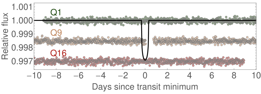
Figure 1.— If the period of KOI-1274.01 were half that which we claim here, three additional transits would occur in the Kepler time series. For a linear ephemeris, the black line shows the expected location of such an event, which is highly inconsistent with the available data (circles).

In a similar vein, it is possible to exclude higher integer ratios. For example, if the true period were a third of our candidate value, four additional transits would occur in the Kepler time series which again the excellent temporal coverage excludes. Accordingly, we are able to demonstrate that our candidate orbital period for KOI-1274.01, of $704.2$ days, is correct.

2.7. Stellar Rotational Period

Stars with active regions have a non-uniform surface brightness distribution, which leads to time variable changes in brightness as the star rotates (Budding, 1977). In practice, these active regions may evolve in location and amplitude over timescales of days to years, and even present evolving periodicities due to differential rotation (Reinhold et al., 2013). Despite this, the rotation period tends to produce a dominant peak in the frequency-domain allowing for an estimate of the rotation period using photometry alone (Basri et al., 2011).

Since the data are unevenly sampled and each quarter has a unique offset, we elected to use a Lomb-Scargle style periodogram. The light curve model is a simple sinusoid and thus is linear with respect to the model parameters, for any trial rotation period, $P_{\mathrm{rot}}$. Using weighted linear least squares, we are guarenteed to find the global maximum likelihood solution at each trial $P_{\mathrm{rot}}$. We scan in frequency space from twice the cadence ($\sim 0.04$ d) up to twice the total baseline of observations ($\sim 2940$ d) making $10^{5}$ uniform steps in frequency. At each realization, we define the “power” as $(BIC_{\mathrm{null}}-BIC_{\mathrm{trial}})/BIC_{\mathrm{null}}$, where BIC is the Bayesian Information Criterion and “null” and “trial” refer to the two models under comparison.

The resulting periodogram, shown in Figure 2, reveals a strong peak at around 30 days. Conducting a second periodogram with a finer grid around this solution and defining the period uncertainty as the full width at half maximum, we find $P_{\mathrm{rot}}=28.5\pm 0.3$ days. We note that this period lies close to the rotation period of typical spots on the surface of the Sun of 27.3 days. This information is used in §3.5 to constrain the age of Kepler-421.

Folding the detrended Kepler photometry on our maximum likelihood rotation period reveals a quasi-sinusoidal pattern, with a peak-to-peak amplitude of $\sim 40$ ppm (see Figure 3).

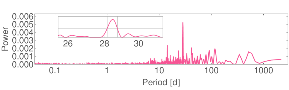
Figure 2.— Periodogram of the Kepler photometry for Kepler-421. A zoomed-in view of the peak at $P=28.5\pm 0.3$ days is shown in the top-left, which we consider to be the stellar rotation period.

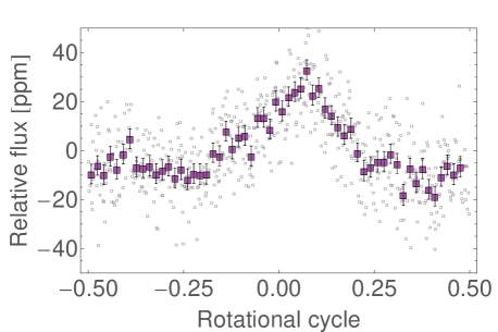
Figure 3.— Out-of-transit Kepler photometry for Kepler-421 folded upon our maximum likelihood rotation period of $28.5$ days. Gray points are 100-point phase binned, purple points are 1000-point phase binned.

3. FOLLOW-UP OBSERVATIONS

3.1. Overview

We describe here further observations and analyses we performed to both characterize the parent star, and to aid in addressing the probability that the photometric signal we detected might be due to an astrophysical false positive (i.e. other phenomena mimicking the transit) rather than a true planet around KOI-1274.

3.2. Spectroscopy

A high-resolution optical spectrum of KOI-1274 was obtained on 2011 August 4 using the fiber-fed echelle Spectrograph (FIES) on the 2.5 m Nordic Optical Telescope (NOT) on La Palma, Spain (Djupvik & Andersen, 2010). The resolving power delivered by the instrument with the medium (1$\farcs$3) fiber setup is $R=46,\!000$, and the 21-minute exposure yielded an average signal-to-noise ratio per resolution element of 35 in the Mg I b region (5190 Å).

On 2012 June 25 we acquired an additional high-resolution spectrum with the Keck I Telescope on Mauna Kea (HI) and its HIRES spectrometer (Vogt et al., 1994). The exposure time was 10 min, and the size of the spectrograph slit was set to 0$\farcs$86. Use of the standard setup and reduction procedures of the California Planet Search (Howard et al., 2010; Johnson et al., 2010) resulted in a spectrum with $R\sim 60,\!000$ covering the range 3642–7990 Å, with a signal-to-noise ratio per resolution element of 56 also in the Mg I b region. The absolute radial velocity of the target was measured from this spectrum using telluric lines as the reference, and is $-25.4\pm 0.1$ $\mathrm{km}\,\mathrm{s}^{-1}$. We note that this is compatible with that derived using the FIES spectrum, $-25.5\pm 0.1$ $\mathrm{km}\,\mathrm{s}^{-1}$.

We used the better-quality HIRES spectrum to search for signs of absorption lines from another star that might be causing the transit signal, by subtracting a spectrum closely matching that of the target star (after proper Doppler shifting and continuum normalization) and inspecting the residuals (Kolbl et al. 2014, in prep). The closest match (in a $\chi^{2}$ sense) was selected from a large library of observed spectra taken with the same instrument, spanning a wide range in temperature, surface gravity, and chemical composition. No evidence of secondary spectral lines was seen. To better quantify our sensitivity to faint companions, we subjected the residuals to a similar fitting process by injecting mock companions over a range of temperatures between 3500 K and 6000 K, and with a wide range in relative velocities, and attempting to recover them. In this way we estimated we are sensitive to companions down to 1% of the flux of the primary star, and velocity separations $\Delta RV$ greater than 10 $\mathrm{km}\,\mathrm{s}^{-1}$. For smaller relative velocities the secondary lines would be blended with those of the primary and would not be detected.

3.3. High-resolution imaging

KOI-1274 was observed as part of a large survey of Kepler Objects of Interest by Law et al. (2013) using a robotic laser-guide-star adaptive optics system known as Robo-AO, on the Palomar 60-inch telescope. Images obtained on 2012 August 6 in the Sloan $i$ passband revealed a close companion with a signal-to-noise ratio of 7, located at an angular separation of $1\farcs 10\pm 0\farcs 06$ in position angle $241\arcdeg\pm 1\arcdeg$. This star is $3.75\pm 0.44$ magnitudes fainter than the target. Law et al. (2013) performed Monte Carlo simulations in order to quantify the sensitivity to additional fainter companions as a function of angular separation, by injecting and then attempting to recover fake stars out to separations of 2$\farcs$5 for a group of representative targets. For our BLENDER analysis below in §4 we have adopted their sensitivity curve corresponding to observations of similar quality as KOI-1274 (see their Figure 5, for medium performance).

3.4. Centroid motion analysis

To search for false positives that may result, e.g., from a background eclipsing binary in the photometric aperture of KOI-1274 we measured the location of the transit signal relative to KOI-1274 via difference images formed by subtracting an average of in-transit pixel values from out-of-transit pixel values. If the transit signal is due to a stellar source, the difference image will show that stellar source, whose location is determined via Pixel Response Function (PRF) centroiding (Bryson et al., 2013). The centroid of an average out-of-transit image gives the location of KOI-1274 because the object is well isolated. The difference image centroid was compared to the out-of-transit image centroid, giving the location of the transit source relative to KOI-1274. This was done for each of the two quarters in which a transit occurs. For further details of the procedure, see Bryson et al. (2013).

In Quarter 5 the measured transit location is offset from KOI-1274 by $0\farcs 532\pm 0\farcs 026$ with a position angle of about 316°. In Quarter 13 the transit location is offset by $0\farcs 065\pm 0\farcs 027$ with a position angle of about 177°. The uncertainties in these quarterly measurements are based on standard propagation of errors starting with the measured pixel-level noise. Clearly there is additional bias in each quarterly centroid measurement, so to determine the transit source location from these two measurements an average was computed as a least-squares constant fit to the quarterly offsets. The uncertainty of this average was computed both via standard propagation of errors for the fit and via a bootstrap estimate. We adopted the larger of these two uncertainty estimates (for details see Bryson et al. (2013)). The resulting average transit signal offset from KOI-1274 is $0\farcs 248\pm 0\farcs 279$ with a position angle of about 308°. This average position estimate is 4.18 $\sigma$ from the companion star at 1$\farcs$1 detected by Law et al. (2013), ruling out that companion as the cause of the transit signal. Based on the 1 $\sigma$ uncertainty in this average we adopt a 3 $\sigma$ radius of confusion of 0$\farcs$84, within which the centroid motion analysis is insensitive to the presence of contaminating stars (blends).

3.5. Stellar properties

The spectroscopic parameters of KOI-1274 were derived from the observations described in §3.2 using the Stellar Parameter Classification pipeline (SPC; Buchhave et al., 2012). Briefly, this algorithm cross-correlates the observed spectra against a large library of calculated spectra based on model atmospheres by R. L. Kurucz spanning a wide range of parameters, and assigns stellar properties interpolated among those of the synthetic spectra giving the best match. There is excellent agreement between the SPC results from the individual spectra. The weighted mean of the two estimates yielded $T_{\rm eff}=5308\pm 50$ K, ${\rm[m/H]}=-0.25\pm 0.08$ dex, $\log g=4.61\pm 0.10$ dex, and $v\sin I_{\star}=0.0\pm 0.5$ $\mathrm{km}\,\mathrm{s}^{-1}$. These parameters correspond to a dwarf star of spectral type G9 or K0.

We determined the mass and radius of the star, along with other characteristics, by comparing these spectroscopic properties with stellar evolution models from the Dartmouth series (Dotter et al., 2008) in a $\chi^{2}$ fashion. The procedure was analogous to that described by Torres et al. (2008). The results are listed in Table 1. The distance estimate of 320 pc relies on an average $V$ magnitude of $13.56\pm 0.04$ (Droege et al., 2006; Henden et al., 2012; Everett et al., 2012) as well as our estimate of the interstellar extinction toward KOI-1274. We inferred the latter from several sources (Hakkila et al., 1997; Schlegel et al., 1998; Drimmel et al., 2003; Amores & Lepine, 2005) that yield an average reddening of $E(B-V)=0.036\pm 0.022$ (conservative error), corresponding to $A_{V}=0.11\pm 0.07$.

The uncertainty in the spectroscopic surface gravity is large enough that the age of the star is essentially unconstrained by the models. However, in §2.7 we describe the detection of a rotation signature in the Kepler photometry with a period of $P_{\rm rot}=28.5\pm 0.3$ days, which enables us to infer an age using gyrochronology relations. We obtain consistent estimates of $3.7_{-0.5}^{+0.9}$ Gyr (Barnes, 2007), $4.1_{-0.6}^{+1.0}$ Gyr (Mamajek & Hillenbrand, 2008), and $4.3_{-0.7}^{+2.9}$ Gyr (Meibom et al., 2009), in which we have adopted a dereddened $B-V$ color of $0.73\pm 0.04$ for the star (from the indices derived by Henden et al. 2012 and Everett et al. 2012, and the above reddening value).

Table 1Stellar properties of KOI-1274.

Property	Value
$T_{\rm eff}$ (K)	$5308\pm 50$
$\log g$ (dex)	$4.61\pm 0.10$
${\rm[Fe/H]}$ (dex)	$-0.25\pm 0.08$
$v\sin I_{\star}$ (km s-1)	$0.0\pm 0.5$
$M_{\star}$ ($M_{\odot}$)	$0.794\pm 0.030$
$R_{\star}$ ($R_{\odot}$)	$0.757\pm 0.029$
$L_{\star}$ ($L_{\odot}$)	$0.40\pm 0.06$
$M_{V}$ (mag)	$5.90\pm 0.12$
Distance (pc)	$320\pm 20$
Age (Gyr)	$4.0\pm 0.8$

4. STATISTICAL VALIDATION

4.1. Overview

A typical mass for a planet the size of KOI-1274.01 ($\sim$4 $R_{\oplus}$) is expected to be 10–20 $M_{\oplus}$, based on the range of properties of known exoplanets. The Doppler signal induced on the host star would then have a semi-amplitude of only 0.8–1.6 $\mathrm{m}\,\mathrm{s}^{-1}$, making it very challenging to detect with current instrumentation around such a faint star ($V=13.58$), particularly given the long orbital period. Dynamical “confirmation” in the usual sense (by establishing that the orbiting object is of planetary mass) is therefore not currently possible in this case. Instead, we describe here our efforts to “validate” it statistically, by showing that the likelihood of a true planet around KOI-1274 is orders of magnitude larger than that of a false positive.

The main type of false positive that can mimic the transit signal in this case involves blends with another eclipsing object in the photometric aperture of Kepler. This includes background eclipsing binaries (‘BEBs’), background or foreground stars transited by a (larger) planet (‘BP’), or physically associated stellar companions transited by another star or by a planet. The companions in these latter cases are generally close enough to the target that they cannot be resolved with high-resolution imaging. We refer to these hierarchical triple configurations as ‘HTS’ and ‘HTP’, respectively, depending on whether the orbiting object is a star or a planet. In each of the four scenarios described above the eclipses are attenuated by the light of the target and can be reduced to planetary proportions, leading to confusion. Other types of false positives not involving contamination by another object include grazing eclipsing binaries, and transits of a small star in front of a giant star. Each of these can easily ruled out because their signals would be inconsistent with the significant second-to-third contact transit duration ($T_{23}=14.18_{-0.15}^{+0.12}$ hours; see §5.1) and the measured properties of the star ($\log g=4.61\pm 0.10$ dex).

To address the blends we relied on the BLENDER technique (Torres et al., 2004, 2011; Fressin et al., 2012), which uses the detailed shape of the transit light curve to weed out scenarios that lead to the wrong shape for a transit. BLENDER simulates large numbers of false positives over a wide range of stellar (or planetary) parameters, and compares their synthetic light curves with the Kepler photometry in a $\chi^{2}$ sense. Blends that provide poor fits are considered to be excluded. This allows us to place tight constraints on the types of objects composing the eclipsing pair that yield viable blends, including their sizes or masses, as well as other properties of the blends such as their overall brightness and color, the linear distance between the background/foreground eclipsing pair and the KOI, and even the eccentricities of the orbits. For details of the procedure we refer the reader to the above sources, or recent applications of BLENDER by Borucki et al. (2013), Meibom et al. (2013), and Ballard et al. (2013). Following the nomenclature in those studies, the objects in the eclipsing pair are designated as the “secondary” and “tertiary”, and the target itself is referred to as the “primary”. Secondary and tertiary stellar properties (masses, sizes, and absolute brightness in the Kepler and other passbands) were drawn from model isochrones from the Dartmouth series (Dotter et al., 2008), and the properties adopted for the primary are those reported in §3.5, supplemented with others inferred from the adopted isochrone. The long-cadence photometry we used for KOI-1274 was processed and detrended as described earlier.

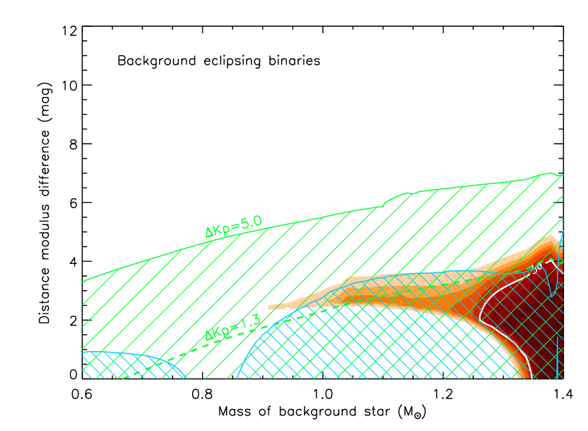
Figure 4.— Map of the $\chi^{2}$ surface (goodness of fit) for KOI-1274.01 corresponding to blends involving background eclipsing binaries. On the vertitcal axis is represented the linear distance between the BEB and the target ($D_{\rm BEB}-D_{\rm targ}$), expressed for convenience in terms of the difference in distance modulus, $\Delta\delta=5\log(D_{\rm BEB}/D_{\rm targ}$). Only blends within the solid white contour (darker colors) provide fits to the Kepler light curve that are within acceptable limits (3$\sigma$, where $\sigma$ is the significance level of the $\chi^{2}$ difference compared to a transiting planet model fit; see Fressin et al., 2012). Other concentric colored areas (lighter colors) represent fits that are increasingly worse (4$\sigma$, 5$\sigma$, etc.), which we consider to be ruled out. The blue cross-hatched areas correspond to regions of parameter space where the blends are either too red (left) or too blue (right) compared to the measured $r-K_{s}$ color of the target, by more than three times the measurement uncertainty. The dashed green line labeled $\Delta K\!p=1.3$ is tangent to the white contour from above and corresponds to the faintest viable blends. The green line labeled $\Delta K\!p=5.0$ represents the spectroscopic limit on faint background stars. All simulated blends below this line (hatched region) are brighter and are generally excluded if the BEB is angularly close enough to the target to fall within the slit of the spectrograph (see text). Thus, very few blends remain viable.

4.2. Blend Frequency

Our simulations with BLENDER rule out all scenarios in which a pair of eclipsing stars orbits the target (HTS). The resulting light curves invariably have the wrong shape for the transit, or produce secondary eclipses that are not observed in the photometry of KOI-1274. Background eclipsing binaries with two stellar components are only able to produce viable false positives if the secondaries are restricted to a very narrow range of masses between about 1.25 $M_{\odot}$ and 1.43 $M_{\odot}$, as well as a limited interval in brightness ($K\!p$ magnitude) relative to the primary ($\Delta K\!p\lesssim 1.3$). We illustrate this in Figure 4, which shows the $\chi^{2}$ landscape for all blends of this kind in a representative cross-section of parameter space. Regions outside of the 3-$\sigma$ contour correspond to configurations with light curves that give poor fits to the Kepler photometry, i.e., much worse than a true planet fit. These scenarios are therefore excluded. Other constraints available for KOI-1274 place further restrictions on viable blends. In particular, comparing the $r-K_{s}$ colors of the simulated blends with the measured color index of the target ($r-K_{s}=1.779\pm 0.023$; Brown et al., 2011), we find that most of the BEB scenarios allowed by BLENDER are too blue by more than 3$\sigma$, and are therefore also excluded. Additionally, the analysis of our Keck/HIRES spectrum generally rules out companions within 5 magnitudes of the primary if they are closer than 0$\farcs$43 (half-width of the spectrograph slit) and their radial velocity (RV) is offset by more than 10 $\mathrm{km}\,\mathrm{s}^{-1}$ from that of the primary. If $\Delta RV<10$ $\mathrm{km}\,\mathrm{s}^{-1}$ line blending could prevent their detection, so those stars are not necessarily excluded. Stars brighter than $\Delta K\!p=5$ but outside of 0$\farcs$43 are only ruled out if they are above the detection threshold from the high-resolution imaging, which is a function of their angular separation. We show these two observational constraints in Figure 4. Other constraints are discussed below.

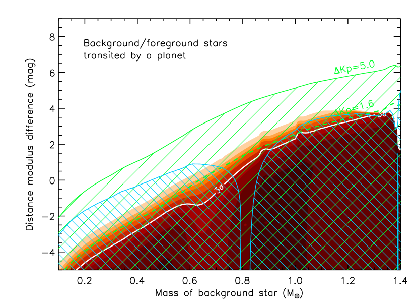
Figure 5.— Similar to Figure 4 (and with the same color scheme) for blends involving background or foreground stars transited by a planet (BP). The faintest blends giving acceptable fits have $\Delta K\!p=1.6$ relative to the target (dashed green line), and are all excluded by the spectroscopic constraint ($\Delta K\!p=5.0$, hatched green area) unless the intruding star is more than 0$\farcs$43 from the target, or within 0$\farcs$43 but with $\Delta RV<10$ $\mathrm{km}\,\mathrm{s}^{-1}$ (see text).

For blend scenarios involving a background or foreground star transited by a planet (BP) there is a wide range of secondary masses that yield acceptable fits to the Kepler light curve, as shown in Figure 5. The faintest of these blends are 1.6 mag fainter than the primary in the $K\!p$ band. However, as in the case of BEBs, the observational constraints severely limit the pool of viable false positives. In particular, many of them are either too red or too blue compared to the measured color index of the target, or are bright enough that they would generally have been detected spectroscopically (but not always; see above).

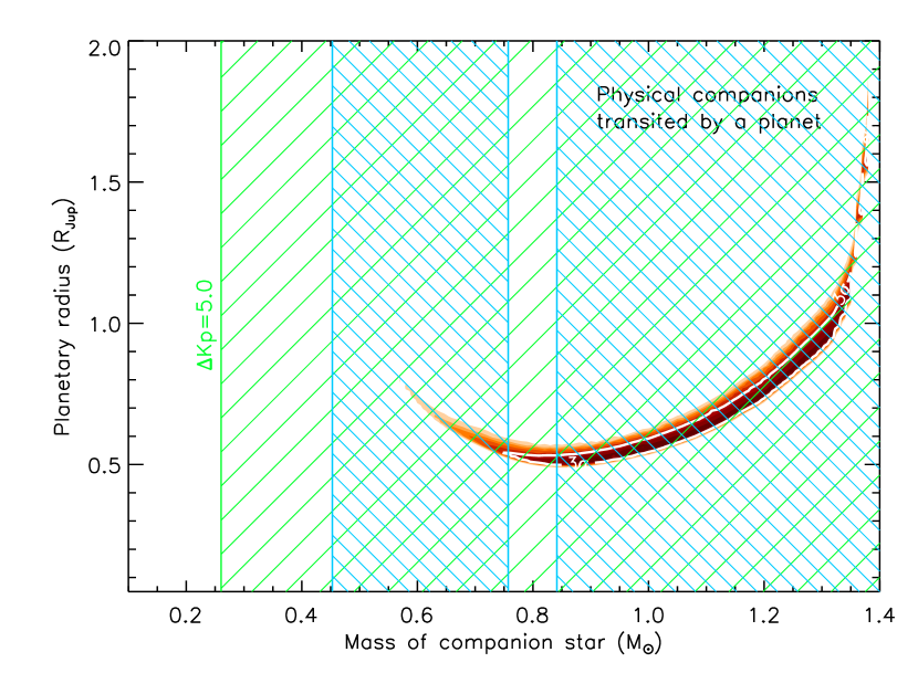
Figure 6.— Similar to Figure 4 for the case of physical companions to KOI-1274 that are transited by a planet (HTP). Only companion stars with masses between about 0.75 $M_{\odot}$ and 0.84 $M_{\odot}$ (i.e., very similar to the target star itself) yield blend colors that are consistent with the measured $r-K_{s}$ index of KOI-1274. However, these blends are generally eliminated by the spectroscopic consraint (but not always; see text), as they are brighter than $\Delta K\!p=5.0$.

The $\chi^{2}$ map for scenarios involving a physically associated companion to KOI-1274 that is transited by a larger planet (HTP) appears in Figure 6, and shows the size of the planetary tertiary that can mimic the transit signal as a function of the companion star. BLENDER restricts viable blends to be in a very narrow strip of parameter space corresponding to secondary masses between about 0.75 $M_{\odot}$ and 1.35 $M_{\odot}$, and planetary sizes 0.5–1.2 $R_{\rm Jup}$ (5.5–13.5 $R_{\oplus}$). As before, color and brightness constraints permit us to exclude most of these blends (see Figure 6), but not all (e.g., not ones within 0$\farcs$43 where the spectral lines of the companion and the primary would be blended).

The frequencies with which each of the blend configurations are expected to occur were computed via Monte Carlo experiments, in which we simulated large numbers of blends and rejected those that give poor fits to the transit photometry or that would have been detected with the aid of our follow-up observations. We then counted the remaining blends to derive their frequencies. These experiments relied on a number of ingredients including the known distributions of binary star properties, the number density of stars near the target, and the rates of occurrence of transiting planets and eclipsing binaries inferred from the Kepler observations themselves. Those rates (and any dependence they may have on orbital period or other properties) are conveniently implicit in the KOI lists generated by the Kepler team and in the eclipsing binary catalog of Slawson et al. (2011), when normalized by the total number of targets observed by Kepler. We have taken advantage of that information below.

For the HTP case we simulated companion stars following the distributions of binary properties given by Raghavan et al. (2010) (mass ratios, orbital periods, eccentricities), and placed them in random orbits around the primary and at random orbital phases. We derived their relevant stellar properties (size, brightness, colors) from the isochrone used for the target. We assigned to each of these companions a random transiting planet drawn from the KOI list hosted at the NASA Exoplanet Archive (downloaded 2014 March 26), but accepted as viable only those with periods similar to that of KOI-1274.01 (within a factor of two). The rationale for this is that the relevant blend frequency is that of configurations involving planets with periods near that of the candidate, since those frequencies depend strongly on period. We then examined the properties of the companion stars and their planets, and rejected configurations that do not satisfy the BLENDER restrictions on companion mass, planetary size, and orbital eccentricity as illustrated in Figure 6. We further rejected those that would have been detected in our high-resolution imaging, spectroscopy, centroid motion analysis, or by their colors. In applying the spectroscopic constraint we discarded blends brighter than $\Delta K\!p=5.0$ mag if the companion star is within 0$\farcs$43 of the target, unless its radial velocity computed from the simulated orbit around the target is within 10 $\mathrm{km}\,\mathrm{s}^{-1}$ of that of KOI-1274. In that case the spectral lines would be heavily blended with those of the primary and might be missed, so we consider those blends still viable. Finally, we retained only configurations that are dynamically stable according to the criterion of Holman & Wiegert (1999). We repeated this experiment a large number of times, counting the surviving blends and finally multiplying by the 46% frequency of non-single stars from Raghavan et al. (2010). The resulting HTP blend frequency is very small, $4.9\times 10^{-11}$, which is due to a combination of very strong observational constraints, the well-defined shape of the transit, and the rare occurrence of larger transiting planets in such wide orbits that can be involved in blends.

The calculation of the frequency of background or foreground stars transited by a planet (BP) proceeded in a similar fashion, and depends on the number density of stars in the vicinity of KOI-1274 (stars per square degree). Using the Galactic structure model of Robin et al. (2003), we began by generating a list of simulated stars in a 5 square-degree area around the target, including their kinematic properties (radial velocity). We then drew stars randomly from this list assigning them a random angular separation from the target within the 0$\farcs$84, 3-$\sigma$ exclusion radius from our centroid motion analysis (since stars outside of this area would have been detected). To each of these stars we assigned a transiting planet from the KOI list, retaining only those within a factor of two of the period of KOI-1274.01, as before. Blends involving background/foreground stars and their planets that do not meet the BLENDER constraints were rejected, along with those that would have been flagged by our follow-up observations (imaging, spectroscopy, and color). We retained configurations in which the velocity of the simulated secondaries are within 10 $\mathrm{km}\,\mathrm{s}^{-1}$ of that measured for KOI-1274 ($-24.7$ $\mathrm{km}\,\mathrm{s}^{-1}$; Sect. 3.1), which would be spectroscopically undetectable. The resulting frequency of false positives of this kind, after normalizing by the ratio of areas between the centroid exclusion region and 5 square degrees, is only $3.5\times 10^{-14}$. The contribution of these kinds of blends to the overall frequency is therefore negligible, and as before this is partly a consequence of how uncommon long-period transiting planets are, which in turn has to do with the low probability of transit.

To assess the frequency of BEBs acting as blends we used the Galactic structure model of Robin et al. (2003) as above, drawing secondaries and assigning a companion star (tertiary) from the distributions of binary properties of Raghavan et al. (2010). We assigned periods to these blends drawn randomly from the list of Kepler binaries by Slawson et al. (2011), and kept only those within a factor of two of the period of KOI-1274.01. After filtering out BEBs with properties that make them inviable according to BLENDER, we applied the observational constraints in the same way as for the BP scenario, and counted the surviving blends. Their frequency in this case is so small that we can only place an upper limit of $\sim 10^{-14}$. In this case the smallness of the number is related to the low frequency of eclipsing binaries with periods as long as 704 days (again largely a result of the low probability of eclipse).

The total blend frequency is the sum of the HTP, BP, and BEB contributions, or $4.9\times 10^{-11}$. While this is a very small figure, the a priori frequency of a true transiting planet such as KOI-1274.01(‘planet prior’) is also expected to be very small. Our aim in the present work is to validate the candidate to a very high level of confidence equivalent to a 3$\sigma$ significance, consistent with previous applications of BLENDER. For this we require a planet prior that is at least $1/(1-99.73\%)\approx 370$ times larger than the total blend frequency, or $\sim 2\times 10^{-8}$.

4.3. Planet Prior

We here discuss our estimation of the a priori probability of Kepler detecting a genuine planet similar to KOI-1274.01- the planet prior. We define the planet prior as the prior probability of a star having a planet similar to KOI-1274.01 (the occurrence rate) multiplied by the prior probability of Kepler detecting such a planet in transit (the detection probability). We discuss each of these in what follows.

4.3.1 Occurrence rate calculation

The occurrence rate of a planet at a specific orbital period and size cannot be reasonably defined, since it will always be infinitessimal. Instead, one must consider a confidence interval defining “similar” planets to the one in question, and then integrate the occurrence rate distribution over this range. For consistency with previous BLENDER works, we define the period interval as $P/2\to 2P$, where $P$ is the orbital period equal to 704.1984 d (see §5). Similarly, previous BLENDER works have defined the size interval to be the 3 $\sigma$ confidence region of $R_{P}$, which for KOI-1274.01 is $3.55$ $R_{\oplus}<R_{P}<5.03$ $R_{\oplus}$ (see §5).

Unlike previous BLENDER analyses (Torres et al., 2011; Fressin et al., 2011, 2012), we are unable to use the Kepler statistics themselves (Fressin et al., 2013) to define the occurrence rate, since these are only complete up to 418 d. Instead, we turn to the radial velocity occurrence rates from Cumming et al. (2008), which are complete for $P<2000$ d and $M_{P}\geq 0.3$ $M_{J}$. One complication introduced by this decision is that we must convert radii to masses. Although empirical mass-radius relations have been derived for $\sim 4$ $R_{\oplus}$ planets (Weiss & Marcy, 2014), these relations are calibrated to planets which are closer to their host star than KOI-1274.01. Instead, given that KOI-1274.01 most closely resembles Uranus in size at just 2.5% larger and both worlds are “cold”, being $\lesssim 200$ K, we simply adopt the Uranian mean density (1.27 g cm^-3) to estimate masses. This changes our 3 $\sigma$ confidence interval from $3.55$ $R_{\oplus}<R_{P}<5.03$ $R_{\oplus}$ to $10.0$ $M_{\oplus}<M_{P}<29.4$ $M_{\oplus}$ (with the most likely value being $16.0$ $M_{\oplus}$).

This mass estimation process reveals that KOI-1274.01 likely has a mass below 0.3 $M_{J}$ ($=95$ $M_{\oplus}$), which is a problem given that the Cumming et al. (2008) relation only extends down to 0.3 $M_{J}$. However, we also know that empirically determined occurrence rates consistently show that smaller planets outnumber their bigger brothers (Jiang et al., 2010). We may therefore simply push our mass range up to the 0.3 $M_{J}$ boundary and any derived occurence rate will be a conservative estimate. This “push” could be done by multiplying the mass range until the lower limit equals 0.3 $M_{J}$ giving $0.30$ $M_{J}<M_{P}<0.85$ $M_{J}$. Alternatively, one may simply add a constant to both limits until the lower limit equals 0.3 $M_{J}$, giving $0.30$ $M_{J}<M_{P}<0.36$ $M_{J}$. The narrow range of this latter estimate yields a more conservative occurrence rate and so we adopt it from here on.

The Cumming et al. (2008) occurrence rate is described by a power-law function:

$$\mathrm{d}N =CM^{\alpha}P^{\beta}\,\mathrm{d}\log M\,\mathrm{d}\log P$$ (1)

It is this function we must integrate between our defined interval to compute the occurrence rate. Before proceeding, we calculate some example occurrences using this law and the Cumming et al. (2008) estimates and associated uncertainties for $\alpha$ and $\beta$ (we assume they are normally distributed). We consider the range $0.3\to 10$ $M_{J}$ to define the range of “giant planets”. This may be compared to the “giants” bin given by Fressin et al. (2013) of $6\to 22$ $R_{\oplus}$. Using the five longest period intervals presented by Fressin et al. (2013), we show the comparison of these two occurrence rate estimates in Figure 7. The evident close agreement of these two estimates demonstrates the reliability of the Cumming et al. (2008) power-law. Accordingly, we use the law to finally estimate a conservative occurrence rate of $0.041_{-0.020}^{+0.038}$% for planets similar to KOI-1274.01.

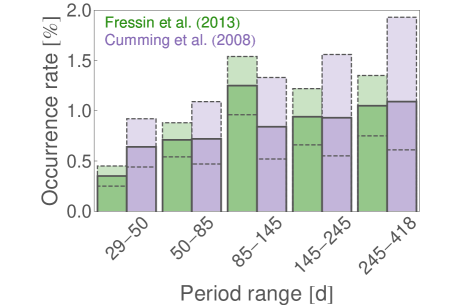
Figure 7.— Occurrence rates of “giant” planets in five period bins from Fressin et al. (2013) (green bars) and Cumming et al. (2008) (purple bars). Dashed lines mark the $\pm 1$ $\sigma$ confidence interval. The Cumming et al. (2008) values provide excellent agreement with those of Fressin et al. (2013), yet extend to longer periods up to 2000 d, thereby offering a viable method of computing the planet prior for KOI-1274.01.

4.3.2 Detection probability calculation

KOI-1274.01 presents a high signal-to-noise ratio (SNR) transit with $(R_{P}/R_{\star})^{2}=(2.508_{-0.058}^{+0.082})\times 10^{-3}$. With a SNR exceeding 40, the recovery rate of such signals is expected to be $\sim 100$% (Fressin et al., 2013). In light of this, the only relevant issue for the detection probability is the geometric transit probability of such a long-period planet. The geometric transit probability of a circular orbit planet is simply $1/(a/R_{\star})$ but circularity cannot be reasonably assumed for a long-period planet such as KOI-1274.01. If one assumes the eccentricity distribution may be described by a Beta distribution (Kipping, 2013a), then the eccentricity-marginalized transit probability is derived by Kipping (2014b) to be

$$\mathrm{P}(\mathrm{transit}|a/R_{\star}) =\Big{(}\frac{1}{a/R_{\star}}\Big{)}\Big{(}\frac{\Gamma[\alpha_{e}+\beta_{e}]}{\beta_{e}-1}\Big{)}\gamma_{1},$$ (2)

$$\gamma_{1} =\,_{2}\tilde{F}_{1}[1,\alpha_{e};\alpha_{e}+\beta_{e}-1;-1],$$ (3)

where $\alpha_{e}$ and $\beta_{e}$ are the Beta distribution shape parameters and ${}_{2}\tilde{F}_{1}$ is Gauss’ hypergeometric function. To compute this probability, we draw samples from the joint posterior distribution of $\alpha_{e}$ and $\beta_{e}$ for the long-period sample described in Kipping (2013a) and samples for $(a/R_{\star})$ from our light curve fits (see §5). This yields $\mathrm{P}(\mathrm{transit}|a/R_{\star})=0.341_{-0.017}^{+0.033}$%.

4.4. Final Result

Using the results of §4.3, we may multiply the planet occurrence rate prior by the transit probability prior to estimate our final planet prior of $(1.41_{-0.69}^{+1.32})\times 10^{-6}$. Recall in §4.2 that any planet prior above $\sim 2\times 10^{-8}$ would indicate a $>3$ $\sigma$ statistical validation of KOI-1274.01. In fact, in this case the probability of a planetary nature for KOI-1274.01 is approximately 28,000 greater than that of a false positive, corresponding to a confidence level for the validation of 4.1$\sigma$. We therefore refer to KOI-1274.01 as Kepler-421b throughout the remainder of this paper, and similarly refer to the host star as Kepler-421.

5. LIGHT CURVE FITS

5.1. Global Fit

Here we here discuss our final transit light curve fit of both epochs (i.e. a global fit) from which we derive our final system parameters. In what follows, we use the detrended PDC Kepler photometric time series as our input data, for which details on the detrending are described in §2.5.

We model the transit light curve using the standard Mandel & Agol (2002) algorithm employing the quadratic limb darkening law. This simple transit model assumes a spherical, opaque planet transiting a spherically symmetric luminous star on a Keplerian orbit. We resample the long-cadence data into short-cadence sampling following the method described in Kipping (2010), to avoid smearing effects. Our model has 10 free parameters in total. These are the orbital period, $P$, the time of transit minimum, $\tau$, the ratio-of-radii, $p$, the mean stellar density, $\rho_{\star}$, the impact parameter, $b$, the orbital eccentricity, $e$, the argument of periapsis, $\omega$, the blend factor, $B$, and the quadratic limb darkening coefficients $q_{1}$ and $q_{2}$. All of these parameters have uniform priors in our fits, except $\rho_{\star}$ which uses a log-normal prior, $e$ which uses a Beta prior, $B$, which uses a normal prior and $\omega$ which uses a periodic uniform prior. Note that we do not fit directly for the standard quadratic limb darkening coefficients $u_{1}$ and $u_{2}$, but rather use the transformed parameters $q_{1}$ and $q_{2}$ as advocated in Kipping (2013b), in order to impose efficient, uninformative and physical priors for the limb darkening profile.

In the case of $\rho_{\star}$, we use an informative log-normal prior rather than an uninformative choice, as used for the other parameters. Using an informative prior in $\rho_{\star}$ allows for the orbital eccentricity to be constrained via Asterodensity Profiling (AP) (Kipping, 2014a), specifically via the photoeccentric effect (Dawson & Johnson, 2012). Using a $\rho_{\star}$ prior from asteroseismology, Kipping et al. (2013b) recently demonstrated this principle on the planet Kepler-22b. In the case of Kepler-421, this dwarf star is too faint ($K\!p=13.354$) for the detection of asteroseismic modes ($K\!p\lesssim 12$) and thus we must find an alternative independent constraint on the stellar density. Recently, Kipping et al. (2014) have proposed that brightness variability on an 8-hour timescale, so-called “flicker” (Bastien et al., 2013), may be used as an alternative constraint for fainter stars. Using the method described in Kipping et al. (2014), we estimate a flicker of $F_{8}=(18.3\pm 5.2)$ ppm which yields a constraint on the stellar density of $\log_{10}(\rho_{\star}\,\mathrm{[kg}\,\mathrm{m}^{-3}\mathrm{]})=(3.08\pm 0.27)$ dex. As discussed in Kipping et al. (2014), a flicker-based estimate of the stellar density has a probability distribution well-described by a log-normal distribution, which is why we use this function here.

In the case of $e$, we use a loose but informative Beta distribution prior described by shape parameters $\alpha_{e}$ and $\beta_{e}$. The Beta distribution provides the closest match to observed distribution of eccentricities from radial velocity surveys (Kipping, 2013a). We use the “long-period” sample $P\gtrsim 1$ year described in Kipping (2013a), described by $\alpha_{e}=1.12$ and $\beta_{e}=3.09$. Beta samples were computed on the fly using the ECCSAMPLES algorithm (Kipping, 2014b). Finally, for the blend prior, we make use of the Robo-AO constrast measurement of the nearby companion (Law et al., 2013), which allows us to account for the extra contaminating light which dilutes the transit depth. In addition to this, we use an extra fixed blend factor unique to each quarter due to contaminating light identified in the MAST database.

We also mention that the out-of-transit baseline flux for each transit epoch is also fitted. However, in this case, we use a linear minimization for the baseline flux, similar to that described by Kundurthy et al. (2011). This treats the baseline flux simply as a nuisance parameter which is not marginalized against, but rather minimized at each Monte Carlo realization. This allows us to reduce the number of free parameters yet retain just 10 model parameters.

To regress our 10-parameter model to the observations, we employed the mulitmodal nested sampling algorithm MultiNest described in Feroz et al. (2008, 2009). We use 4000 live points with constant efficiency mode turned off and set an enlargement factor of 0.1. The maximum a posteriori model parameters and their associated 68.3% credible intervals are provided in Table 2. We also show the folded transit light curve and the maximum a posteriori transit model in Figure 8.

Table 2Final parameter estimates for Kepler-421b. ^† = assuming a Bond albedo similar to Neptune/Uranus of 0.30. ^∗ = equivalent semi-major axis of the Kepler-421b if planet orbited the Sun and received an insolation level of $S_{\mathrm{eff}}$.

Parameter	Estimate
Fitted parameters
$P$	$704.1984_{-0.0016}^{+0.0016}$
$\tau$ [BKJDUTC-2,455,000]	$325.7674_{-0.0012}^{+0.0012}$
$(R_{P}/R_{\star})$	$0.05008_{-0.00059}^{+0.00081}$
$\rho_{\star}$ [g cm-3]	$1.58_{-0.37}^{+0.22}$
$b$	$0.21_{-0.14}^{+0.17}$
$q_{1}$	$0.53_{-0.12}^{+0.16}$
$q_{2}$	$0.311_{-0.095}^{+0.116}$
$e$	$0.041_{-0.034}^{+0.095}$
$\omega$ [∘]	$160_{-120}^{+150}$
Other transit parameters
$(a/R_{\star})$	$346_{-29}^{+16}$
$i$ [∘]	$89.965_{-0.031}^{+0.024}$
$u_{1}$	$0.814_{-0.069}^{+0.057}$
$u_{2}$	$-0.08_{-0.12}^{+0.14}$
$T_{14}$ [hours]	$15.79_{-0.10}^{+0.12}$
$T_{23}$ [hours]	$14.18_{-0.15}^{+0.12}$
$T_{12}\simeq T_{34}$ [hours]	$0.785_{-0.035}^{+0.105}$
Physical parameters
$R_{P}$ [$R_{\oplus}$]	$4.16_{-0.16}^{+0.19}$
$a$ [AU]	$1.219_{-0.106}^{+0.089}$
$T_{\mathrm{eq}}^{\dagger}$ [K]	$184.8_{-4.8}^{+8.6}$
$S_{\mathrm{eff}}$ [$S_{\oplus}$]	$0.276_{-0.028}^{+0.055}$
$a_{\mathrm{eff}}^{*}$ [AU]	$1.90_{-0.17}^{+0.10}$

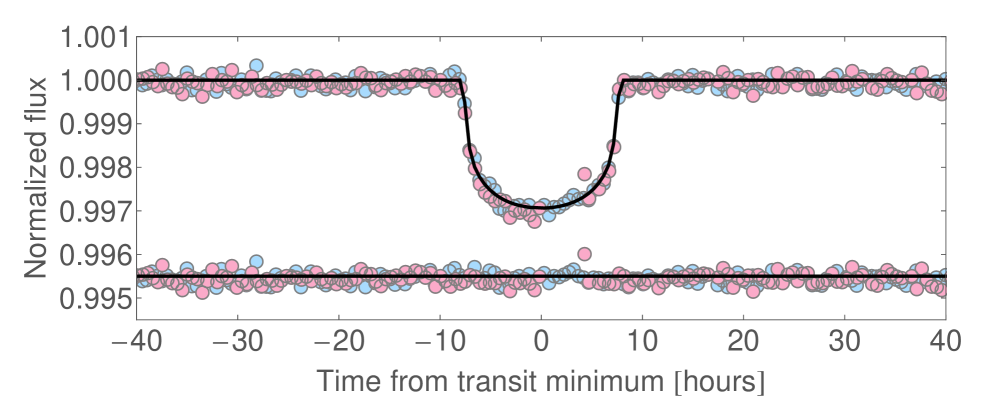
Figure 8.— Folded transit light curve. Blue points are associated with epoch 1, and red points with epoch 2. Maximum a posteriori model fit is shown in solid gray, with the corresponding (offset) residuals shown below.

5.2. Individual Fits

We also attempted independent fits of each of our two individual transits. The purpose of the these fits was to verify quantitatively that the two transits are consistent with being due to the same transiting body (see §2.6). In these fits, it is necessary to fix the orbital period, for which we adopt the maximum a posteriori period from the global fit. Additionally, we fix the two quadratic limb darkening coefficients to values interpolated from the Claret & Bloemen (2011) tabulation of Kepler bandpass coefficients as generated from a PHOENIX stellar atmosphere model. The interpolation is made at the point $T_{\mathrm{eff}}=5308$ K and $\log g=4.632$, giving $u_{1}=0.542$ and $u_{2}=0.139$. Fixing the limb darkening coefficients in these fits imposes the condition that the host star is the same between the two transits, but does not impose that the transiting body is the same.

We regress the standard Mandel & Agol (2002) model to each transit using MultiNest and four free parameters, $\tau$, $p$, $\rho_{\star}$ and $b$, where we use the same priors as before, except $\rho_{\star}$ changes to an uninformative Jeffrey’s prior. We also still enforce the blend factor, $B$, but now simply fix it at the maximum likelihood value rather than imposing a Gaussian prior. As with the limb darkening, this both simplifies the regression and enforces the condition that the star is the same between the two transits.

In Table 3, we report the maximum a posteriori values for these parameters for each epoch, although we replace $b$ and $\rho_{\star}$ with the more intuitive transit durations $T_{14}$ and $T_{23}$. From Table 3, it is evident that the two transits are consistent with being due to the same underlying transiting body, supporting our hypothesis made earlier in §2.6. Also note that there is no evidence for precession effects between these two events.

Table 3 Comparison of the four basic parameters describing a transit when epochs 1 and 2 are fitted independently.

Parameter	Epoch 1	Epoch 2
$\tau$ [BKJDUTC-2,455,000]	$325.7674_{-0.0012}^{+0.0012}$	$1029.9658_{-0.0012}^{+0.0012}$
$(R_{P}/R_{\star})$	$0.04990_{-0.00044}^{+0.00103}$	$0.05057_{-0.00043}^{+0.00092}$
$T_{14}$ [hours]	$15.748_{-0.094}^{0.128}$	$15.774_{-0.089}^{+0.119}$
$T_{23}$ [hours]	$14.122_{-0.171}^{+0.097}$	$14.141_{-0.154}^{+0.090}$

5.3. Exomoon Fits

The long-period nature of Kepler-421b makes an exomoon search provocative, despite the paucity of transit observations. In general, searching for an exomoon around a planet with just a few transits cannot yield a comprehensive search, since during these two events a moon of any size could happen not to transit the star. For this reason, upper limits on a moon’s size are generally very large. With just two transits, deviations from a linear ephemeris cannot be detected and thus the transit timing variations (TTV) effect is lost, which is the easiest way to infer a moon’s mass (Kipping, 2009a, b). Nevertheless, weaker constraints on an exomoon’s mass can be inferred by transit duration variations, TDVs (Kipping, 2009a, b), and ingress/egress asymmetry (Kipping, 2011b). For this reason, a photodynamic algorithm is the most reasonable way to model potential exomoons.

We regressed the analytic photodynamic LUNA transit model (Kipping, 2011b) of a planet with a single moon using the MultiNest algorithm. We adopt the same proceedures and priors as used in previous papers from the “Hunt for Exomoons with Kepler” (HEK) project (e.g. see Kipping et al. 2012, 2013a, 2013b).

By comparing the Bayesian evidences, we find that the planet-with-moon model is favored over the simple planet-only model at 8.3 $\sigma$. However, this significance should not be used in isolation to claim moon detections, as has been cautioned in previous HEK papers. Inspecting the posterior distributions for the 15 parameters in our model (14 usual planet-with-moon parameters used by the HEK project plus one extra for the blend factor $B$) reveals a preference for a short-period, close-in moon with $a_{SP}/R_{P}=3.52_{-0.57}^{+0.73}$ ($a_{SP}=$semi-major axis of the moon around the planet) and $P_{S}=0.339_{-0.007}^{+0.0129}$ days (orbital period of the moon). This is apparent by plotting the maximum a posteriori light curve model shown in Figure 9, where the model produces mutual events (i.e. the moon and planet eclipse during a transit) at several locations, which is the dominant type of photometric effect of close-in moons (Kipping, 2011b).

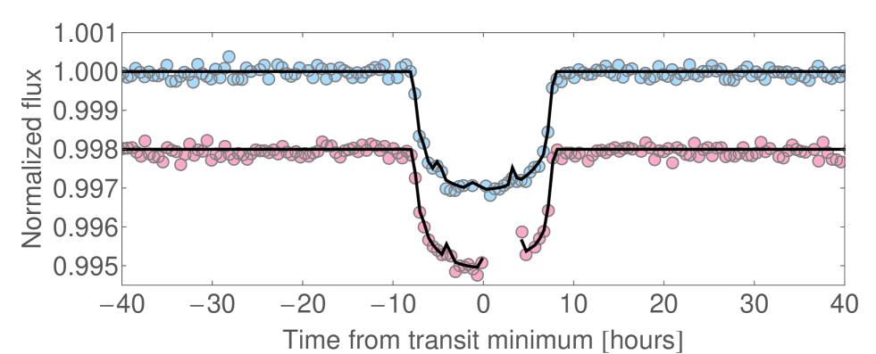
Figure 9.— Maximum a posteriori planet-with-moon light curve model generated using LUNA (Kipping, 2011b) for the Kepler-421b photometry. Blue points show the first transit epoch and red the second (vertically offset by 0.002). We argue that the depicted moon model is likely fitting out starspot crossings.

The light curve features due to mutual events have a close morphological resemblance to starspot crossings (e.g. see Pont et al. 2007; Rabus et al. 2009). The features shown in Figure 9 have an amplitude $\lesssim 300$ ppm, which appears considerably larger than the rotational modulation ampltidue shown later in §2.7. However, the rotational modulations may be caused by a mixture of dark and bright spots leading to an attenuated disk-integrated signal. We therefore consider the hypothesis of starspot crossings to be a viable explanation for the features fitted out by the planet-with-moon model. Without unambiguous evidence for what would be the first observation of a transiting exomoon, the model should be considered to be not the favored hypothesis for this data. We compute a 95% confidence upper limit on the satellite-to-planet mass ratio of $(M_{S}/M_{P})<0.26$, using our marginalized posterior distributions from the photodynamic fit.

6. DISCUSSION

6.1. Insolation

As the longest period known transiting planet, Kepler-421b should be much cooler than the typical transiting exoplanet. The orbit-averaged insolation received by Kepler-421b, $S_{\mathrm{eff}}$, is

$$\frac{S_{\mathrm{eff}}}{S_{\oplus}} =\frac{(L_{\star}/L_{\odot})}{(a_{P}/\mathrm{AU})^{2}\sqrt{1-e^{2}}},$$ (4)

where $S_{\oplus}$ denotes the orbit-averaged insolation received by the Earth. Using our joint posterior distributions for the planetary and stellar parameters, $S_{\mathrm{eff}}=0.276_{-0.028}^{+0.055}$ $S_{\oplus}$. The equilibrium temperature of Kepler-421b is then $T_{P}=202.0_{-5.3}^{+9.5}$ K for a Bond albedo of zero, or $T_{P}=184.8_{-4.8}^{+8.6}$ K using a more realistic assumption of a Uranian-like albedo of 0.30.

With a semi-major axis of $1.22_{-0.11}^{+0.09}$ AU, Kepler-421b orbits closer to its parent star than the orbit of Mars (1.52 AU) around the Sun. Despite this smaller orbit, the lower luminosity of Kepler-421 ($L_{\star}=0.40\pm 0.06$ $L_{\odot}$) causes Kepler-421b to receive just $\sim$64% of the insolation received by Mars (0.43 $S_{\oplus}$). Comparing the incident insolation to the habitable-zone boundaries of Kopparapu et al. (2013), Kepler-421b lies firmly outside the maximum greenhouse outer edge. Statistically, 79% of the joint posterior samples lie beyond the maximum greenhouse outer boundary.

Due to the lower luminosity of Kepler-421, we seek an alternative insolation-weighted metric for comparing the orbit of Kepler-421b with the planetary orbits in the Solar System. We define the “effective semi-major axis” as the semi-major axis of a circular orbit around the Sun where the exoplanet would receive the same insolation as in its current orbit around its host host. Mathematically, we have

$$\frac{a_{\mathrm{eff}}}{\mathrm{AU}} =\sqrt{\frac{1}{(S_{\mathrm{eff}}/S_{\oplus})}},$$ (5)

where $S_{\mathrm{eff}}$ was defined earlier in Equation 4. With this relation, the effective semi-major axis of Kepler-421b is $1.90_{-0.17}^{+0.10}$ AU. Thus, Kepler-421b has an insolation roughly midway between the insolations of Mars and the asteroid Vesta ($a$ = 2.36 AU).

6.2. A Transiting Planet Near the Snow-Line

To place the insolation results in the context of planet formation theories, it is useful to compare $a_{\mathrm{eff}}$ with the location of the snow-line. The snow-line is an annulus in a protoplanetary disk where water ice condenses out of the gas (Sasselov & Lecar, 2000). As the central star approaches the main sequence, time evolution of the disk temperature changes the location of the snow line (Kennedy et al., 2006; Garaud & Lin, 2007; Kennedy & Kenyon, 2008). In most planet formation theories, rocky terrestrial planets form inside the snow line; icy planets grow outside the snow line (Ida & Lin, 2005).

In the Solar System, evidence from the asteroid belt suggests a “canonical” snow-line distance of around 2.7 AU (Abe et al., 2000; Morbidelli et al., 2000; Rivkin et al., 2002). However, the location in a general protoplanetary disk depends upon the luminosity of the central star and the grain opacities, mass accretion rates, and surface densities in the disk (Lecar et al., 2006). Time variations in these quantities change the position of the snow-line. Theoretical calculations of static protoplanetary disks suggest snow-line distances of 1.0–1.8 AU (Sasselov & Lecar, 2000; Lecar et al., 2006). Time-dependent calculations yield distances of 3 AU at 0.3 Myr to 1 AU at 10 Myr (Kennedy & Kenyon, 2008). Our effective semi-major axis of $1.90_{-0.17}^{+0.10}$ AU places Kepler-421b beyond the snow-line for most of the evolution of the protosolar nebula.

To compare the actual semi-major axis of Kepler-421b to protoplanetary disk models, we consider evolving disks around a 0.8 $M_{\odot}$ star (e.g., Kennedy & Kenyon, 2008). The Kennedy & Kenyon (2008) calculations derive the position of the snow line as a function of time in response to changes in the disk accretion rate and the stellar luminosity. We digitized the temporal evolution curves shown in their Figure 1 and then linearly interpolated between the 0.6 $M_{\odot}$ and 1.0 $M_{\odot}$ curves to estimate the location of Kepler-421’s snow-line over time, which is shown in Figure 10.

Using our posterior samples for the semi-major axis of Kepler-421b (i.e. $a$ and not $a_{\mathrm{eff}}$), the orbit of Kepler-421b lies inside the snow-line for stellar ages exceeding $\tau\simeq 2.9_{-0.5}^{+0.9}$ Myr. This age is comparable to the median lifetimes of protoplanetary disks around solar-type stars (e.g., Strom et al., 1993; Haisch et al., 2001). With disk lifetimes scaling as $M_{\star}^{-1/2}$ (Yasui et al., 2012), it is quite feasible that Kepler-421’s protoplanetary disk remained at this time.

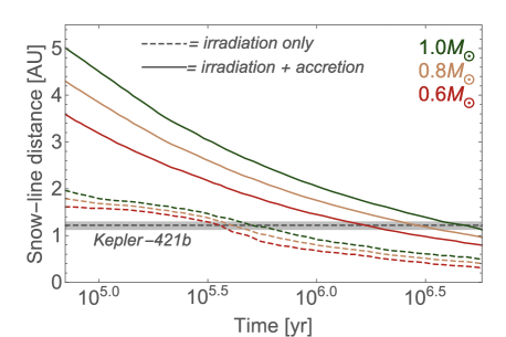
Figure 10.— Location of the snow-line over time for a $0.6$ $M_{\odot}$, $0.8$ $M_{\odot}$ and $1.0$ $M_{\odot}$ star, with irradiation only (using Palla & Stahler 1999 PMS tracks, dashed line) and irradiation + accretion (solid line). Calculated contours come from Kennedy et al. (2006), except for the $0.8$ $M_{\odot}$ contour which is an interpolation between the other two. The 68.3% confidence interval for Kepler-421b’s present location (gray band) equates to the snow-line distance at $\sim 3$ Myr.

Snow-line transiting planets like Kepler-421b may be common but their discovery is impinged by the low transit probability ($\sim 0.3$%) and number of events. Wright et al. (2009) highlighted an enhancement in the occurrence of exoplanets $\sim 1$ AU, which Mordasini et al. (2012) interpret as a signature of the snow-line. Rice et al. (2013) find that by normalizing exoplanet semi-major axes by the snow-line distance, there is evidence for a pile-up of planets around the snow-line threshold, suggesting Kepler-421b-like worlds may be common.

6.3. Formation Scenarios

Although calculating detailed formation scenarios for Kepler-421b is outside the scope of this work, simple arguments suggest Kepler-421b is an icy planet which formed at or beyond the snow line. With a radius of roughly 4 $R_{\oplus}$ and a mass density of at least 5 g cm^-3, a rocky Kepler-421b has a mass of at least 60 $M_{\oplus}$. Growing such a massive planet requires a massive protostellar disk with most of the solid material at 1–2 AU (Mann et al., 2010; Hansen & Murray, 2012). Among protoplanetary disks in nearby star-forming regions, such massive disks are rare (Andrews et al., 2013). Thus, a rocky Kepler-421b seems unlikely.

Outside the snow-line, icy planets with radii of roughly 4 $R_{\oplus}$ can form in more common, much less massive disks. In the standard core accretion theory, icy planets grow from the agglomeration of smaller planetesimals (e.g., Youdin & Kenyon, 2013). Depending on the initial sizes of the planetesimals growth times range from a few Myr to several Gyr (Mann et al., 2010; Bromley & Kenyon, 2011; Kobayashi et al., 2011; Rogers et al., 2011; Lambrechts & Johansen, 2012; Kenyon & Bromley, 2014). As icy planets grow, they migrate through the gas or leftover planetesimals (Ida & Lin, 2005; Mann et al., 2010; Kenyon & Bromley, 2014). Migrating planets sometimes reach small semi-major axes, $a\lesssim 0.5$ AU (Mann et al., 2010; Rogers et al., 2011). Often, the low surface densities of leftover planetesimals preclude migration inside 1–2 AU (Kenyon & Bromley, 2014).

For Kepler-421b, in situ formation is a reasonable alternative to formation and migration from larger semi-major axes. Scaling results from published calculations, the time scale to produce a 10–20 $M_{\oplus}$ planet is comparable to or larger than the median lifetime of the protoplanetary disk (e.g., Mann et al., 2010; Rogers et al., 2011; Lambrechts & Johansen, 2012; Kenyon & Bromley, 2014). Thus, formation from icy planetesimals is very likely. If significant migration through the gas (e.g., Lega et al., 2014) and leftover planetesimals (e.g., Kenyon & Bromley, 2014) can be avoided, Kepler-421b remains close to the “feeding zone” in which it formed.

Developing a more rigorous theory requires more information (see the discussion in Kenyon & Bromley, 2014). Good estimates for the mean density can distinguish between rocky and icy formation scenarios. Detecting absorption from atmospheric constituents might enable choices between various migration scenarios.

6.4. Future Follow-Up

Within the Kepler time series, only two transits of Kepler-421b are observed. The expected third transit would have occurred in March 2014, after the primary Kepler Mission ended. Unfortunately, we did not have time to schedule observations capable of detecting the event. The fourth transit is due at $2,457,438.3627_{-0.0041}^{+0.0042}$ $\mathrm{BJD}_{\mathrm{UTC}}$, which is in February 2016. Note that these estimates assume a strictly linear ephemeris, for which we have no direct evidence given that only two transits have been observed thus far.

Assuming a Uranian mean density for Kepler-421b, we estimate that the radial velocity semi-amplitude induced on Kepler-421 would be $K=1.40_{-0.14}^{+0.20}$ m/s with a periodicity of 704 d. This clearly presents a significant challenge to current observational facilities, but Kepler-421b is a unique object being the first Neptune-like planet discovered at long-period by transits or radial velocity. Determining the mass of the first transiting cold-Neptune would provide a crucial point in intepretting the empirical mass-radius relationship of exoplanets as a function of insolation.

References

- Abe et al. (2000) Abe, Y., Ohtani, E., Okuchi, T., Righter, K. & Drake, M., 2000, Origin of the Earth and Moon, ed. R. M. Canup & K. Righter (Tucson: Univ. Arizona Press), 1, 413
- Akeson et al. (2013) Andrews, R. L. et al., 2013, PASP, 125, 989
- Andrews et al. (2013) Andrews, S. M.,Rosenfeld, K. A., Kraus, A. L. & Wilner, D. J., 2013, ApJ, 771, 129
- Agol (2003) Agol, E., 2003, ApJ, 594, 449
- Amores & Lepine (2005) Amôres, E. B., & Lépine, J. R. D., 2005, AJ, 130, 659
- Baglin et al. (2006) Baglin, A., Michel, E., Auvergne, M. & COROT Team, 2006, in Proc. of the CoRoT Mission Pre-Launch Status—Stellar Seismology and Planet Finding, ed. M. Fridlund, A. Baglin, J. Lochard & L. Conroy (ESA SP-1306; Noordwijk: ESA), 39
- Bakos et al. (2004) Bakos, G. A., Noyes, R. W., Kovacs, G., Stanek, K. Z., Sasselov, D. D. & Domsa, I., 2004, PASP, 116, 266
- Ballard et al. (2013) Ballard, S. et al., 2013, ApJ, 773, 98
- Barnes & Fortney (2004) Barnes, J. W. & Fortney, J. J., 2004, ApJ, 616, 1193
- Barnes (2007) Barnes, S. A., 2007, ApJ, 669, 1167
- Basri et al. (2011) Basri, G. et al., 2011, AJ, 141, 20
- Bastien et al. (2013) Bastien, F. A., Stassun, K. G., Basri, G. & Pepper, J., 2013, Nature, 500, 427
- Batalha et al. (2013) Batalha, N. et al., 2013, ApJS, 204, 21
- Beatty & Gaudi (2008) Beatty, T. G. & Gaudi, S. B., 2008, ApJ, 686, 1302
- Bodenheimer et al. (2000) Bodenheimer, P., Hubickyj, O. & Lissauer, J. J., 2000, Icarus, 143, 2
- Borucki et al. (2009) Borucki, W. et al., 2008, in Pont F., Sasselov, D., Holman M. J., eds, Proc. IAU Symp. 253: Transiting Planets, p. 289
- Borucki et al. (2013) Borucki, W. J. et al., 2013, Science, 340, 587
- Bromley & Kenyon (2011) Bromley, B. C. & Kenyon, S. J., 2011, ApJ, 731, 101
- Brown et al. (2011) Brown, T. M., Latham, D. W., Everett, M. E., & Esquerdo, G. A., 2011, AJ, 142, 112
- Bryson et al. (2013) Bryson, S. T. et al., 2013, PASP, 125, 889
- Buchhave et al. (2012) Buchhave, L. A. et al., 2012, Nature, 486, 375
- Budding (1977) Budding, E., 1977, Ap&SS, 48, 207
- Burke et al. (2014) Burke, C. J. et al., 2014, ApJS, 210, 19
- Charbonneau et al. (2000) Charbonneau, D., Brown, T. M., Latham, D. W. & Mayor, M., 2000, ApJ, 529, L45
- Claret & Bloemen (2011) Claret, A, & Bloemen, S., 2011, A&A, 529, 75
- Cumming et al. (2008) Cumming, A., Butler, R. P., Marcy, G. W., Vogt, S. S., Wright, J. T. & Fischer, D. A., 2008, PASP, 120, 531
- Dawson & Johnson (2012) Dawson, R. I. & Johnson, J. A., 2012, ApJ, 756, 13
- Djupvik & Andersen (2010) Djupvik, D. D. & Andersen, J., 2010, Highlights of Spanish Astrophysics V, J. M. Diego, L. J. Goicoechea, J. I. González-Serrano, & J. Gorgas, eds., p. 211
- Dotter et al. (2008) Dotter, A., Chaboyer, B., Darko, J., Veselin, K., Baron, E., & Ferguson, J. W., 2008, ApJS, 178, 89
- Drimmel et al. (2003) Drimmel, R., Cabrera-Lavers, A., & López-Corredoira, M., 2003, A&A, 409, 205
- Droege et al. (2006) Droege, T. F., Richmond, M. W., & Sallman, M., 2006, PASP, 118, 1666
- Everett et al. (2012) Everett, M. E., Howell, S. B., & Kinemuchi, K., 2012, PASP, 124, 316
- Feroz et al. (2008) Feroz, F. & Hobson, M. P., 2008, MNRAS, 384, 449
- Feroz et al. (2009) Feroz, F., Hobson, M. P. & Bridges, M., 2009, MNRAS, 398, 1601
- Fressin et al. (2011) Fressin, F. et al., 2011, ApJS, 197, 5
- Fressin et al. (2012) Fressin, F. et al., 2012, Nature, 482, 195
- Fressin et al. (2013) Fressin, F. et al., 2013, ApJ, 766, 81
- Garaud & Lin (2007) Garaud, P. & Lin, D. N. C., 2007, ApJ, 654, 606
- Haisch et al. (2001) Haisch, Jr., K. E., Lada, E. A. & Lada, C. J., 2001, ApJ, 553, L153
- Hakkila et al. (1997) Hakkila, J., Myers, J. M., Stidham, B. J., & Hardmann, D. H., 1997, AJ, 114, 2043
- Hansen & Murray (2012) Hansen, B. M. S. & Murray, N., 2012, ApJ, 751, 158
- Henden et al. (2012) Henden, A. A., Levine, S. E., Terrell, D., Smith, T. C., & Welch, D., 2012, J. American Association of Variable Star Observers, 40, 430
- Holman & Wiegert (1999) Holman, M. J. & Wiegert, P. A., 1999, AJ, 117, 621
- Howard et al. (2010) Howard, A. W., Johnson, J. A., Marcy, G. W. et al., 2010, ApJ, 721, 1467
- Hui & Seager (2002) Hui, L. & Seager, S., 2002, ApJ, 572, 540
- Ida & Lin (2005) Ida, S. & Lin, D. N. C., 2005, ApJ, 626, 1045
- Jiang et al. (2010) Jiang, I.-G., Yeh, L.-C., Chang, Y.-C. & Hung, W.-L., 2010, ApJS, 186, 48
- Johnson et al. (2010) Johnson, J. A. et al., 2010, PASP, 122, 701
- Kennedy et al. (2006) Kennedy, G. M., Kenyon, S. J. & Bromley, B. C., 2006, ApJ, 650, L139
- Kennedy & Kenyon (2008) Kennedy, G. M. & Kenyon, S. J., 2008, ApJ, 673, 502
- Kenyon & Bromley (2014) Kenyon, S. J. & Bromley, B. C., 2014, ApJ, 780, 4
- Kipping (2009a) Kipping, D. M., 2009a, MNRAS, 392, 181
- Kipping (2009b) Kipping, D. M., 2009b, MNRAS, 396, 1797
- Kipping (2010) Kipping, D. M., 2010, MNRAS, 408, 1758
- Kipping (2011a) Kipping, D. M., 2011a, MNRAS, 409, L119
- Kipping (2011b) Kipping, D. M., 2011b, MNRAS, 416, 689
- Kipping et al. (2012) Kipping, D. M., Bakos, G. Á., Buchhave, L. A., Nesvorný, D. & Schmitt, A. 2012, ApJ, 750, 115
- Kipping et al. (2013a) Kipping, D. M., Hartman, J., Buchhave, L. A., Schmitt, A., Nesvorný, D. & Bakos, G. Á., 2013a, ApJ, 770, 101
- Kipping et al. (2013b) Kipping, D. M., Forgan, D., Hartman, J., Nesvorný, D., Bakos, G. Á., Schmitt, A. & Buchhave, L. A., 2013b, ApJ, 777, 134
- Kipping (2013a) Kipping, D. M., 2013a, MNRAS, 434, L51
- Kipping (2013b) Kipping, D. M., 2013b, MNRAS, 435, 2152
- Kipping (2014a) Kipping, D. M., 2014a, MNRAS, 440, 2164
- Kipping (2014b) Kipping, D. M., 2014b, MNRAS, submitted
- Kipping et al. (2014) Kipping, D. M., Bastien, F. A., Stassun, K. G., Chaplin, W. J., Huber, D. & Buchhave, L. A., 2014, ApJ, 785, L32
- Kobayashi et al. (2011) Kobayashi, H., Tanaka, H. & Krivov, A. V., 2011, ApJ, 738, 35
- Kopparapu et al. (2013) Kopparapu, R. K. et al., 2013, ApJ, 765, 131
- Kruse & Agol (2014) Kruse, E. & Agol, E., 2014, Science, 344, 275
- Kundurthy et al. (2011) Kundurthy, P., Agol., E., Becker, A. C., Barnes, R., Williams, B. & Makadam, A., 2011, ApJ, 731, 123
- Lambrechts & Johansen (2012) Lambrechts, M. & Johansen, A., 2012, A&A, 544, 32
- Law et al. (2013) Law, N. M. et al., 2013, ApJ, submitted (astro-ph:1312.4958)
- Lecar et al. (2006) Lecar, M., Podolak, M., Sasselov, D. & Chiang, E., 2006, ApJ, 640, 1115
- Lega et al. (2014) Lega, E., Crida, A., Bitsch, B. & Morbidelli, A., 2014, MNRAS, 440, 683
- Lissauer (2001) Lissauer, J. J. 2001, Nature, 409, 23
- Mamajek & Hillenbrand (2008) Mamajek, E. E. & Hillenbrand, L. A., 2008, ApJ, 687, 1264
- Mandel & Agol (2002) Mandel, K. & Agol, E., 2002, ApJ, 580, 171
- Mann et al. (2010) Mann, A. W., Gaidos, E. & Gaudi, B. S., ApJ, 719, 1454
- Marcy et al. (2014) Marcy, G. W. et al., 2014, ApJS, 210, 20
- Mayor et al. (2011) Mayor, M. et al., 2011, arXiv e-prints:1109.2497
- Meibom et al. (2009) Meibom, S., Mathieu, R. D. & Stassun, K. G., 2009, ApJ, 695, 679
- Meibom et al. (2013) Meibom, S. et al., 2013, Nature, 499, 55
- Morbidelli et al. (2000) Morbidelli, A., Chambers, J., Lunine, J. I., Petit, J. M., Robert, F., Valsecchi, G. B. & Cyr, K. E., 2000, M&PS, 35, 1309
- Mordasini et al. (2012) Mordasini, C., Alibert, Y., Benz, W., Klahr, H. & Henning, T., 2012, A&A, 541, 97
- Muirhead et al. (2013) Muirhead, P. S. et al., 2013, ApJ, 767, 111
- Palla & Stahler (1999) Palla, F. & Stahler, S. W., 1999, ApJ, 525, 772
- Pepper et al. (2007) Pepper, J. et al., 2007, PASP, 119, 923
- Pepper et al. (2012) Petigura, J., Kuhn, R. B., Siverd, R., James, D. & Stassun, K., 2012, PASP, 124, 230
- Petigura et al. (2013) Petigura, E. A., Howard, A. W. & Marcy, G. A., 2013, PNAS, 110, 19273
- Pont et al. (2007) Pont, F. et al., 2007, A&A, 476, 1347
- Rabus et al. (2009) Rabus, M. et al., 2009, A&A, 494, 391
- Raghavan et al. (2010) Raghavan, D. et al., 2010, ApJS, 190, 1
- Rauer et al. (2013) Rauer, H et al., 2013, Exp. Astron., submmited (astro-ph:1310.0696)
- Reinhold et al. (2013) Reinhold, T., Reiners, A. & Basri, G., 2013, A&A, 560, 4
- Rice et al. (2013) Rice, K., Penny, M. T. & Horne, K., 2013, MNRAS, 428, 756
- Ricker et al. (2010) Ricker, G. R. et al., 2010, in American astronomical society meeting abstracts #215, vol. 42 of Bulletin of the American Astronomical Society, p. 450.06
- Rivkin et al. (2002) Rivkin, A. S., Howell, E. S., Vilas, F. & Lebofsky, L. A., 2002, Asteroids III (Tucson, AZ: Univ. Arizona Press), 235
- Robin et al. (2003) Robin, A. C., Reylé, C., Derrière, S., & Picaud, S. 2003, A&A, 409, 523
- Rogers et al. (2011) Rogers, L. A., Bodenheimer, P., Lissauer, J. J. & Seager, S., 2011, ApJ, 738, 59
- Sasselov & Lecar (2000) Sasselov, D. D. & Lecar, M., 2000, ApJ, 528, 995
- Schlegel et al. (1998) Schlegel, D. J., Finkbeiner, D. P., & Davis, M., 1998, ApJ, 500, 525
- Seager & Sasselov (2000) Seager, S. & Sasselov, D. D., 2000, ApJ, 537, 916
- Sidis & Sari (2011) Sidis, O. & Sari, R., 2011, ApJ, 720, 904
- Slawson et al. (2011) Slawson, R. W. et al., 2011, AJ, 142, 160
- Street et al. (2003) Street, R. A. et al. 2003, in ASP Conf. Ser. 294, Scientific Frontiers in Research on Extrasolar Planets, ed. D. Deming & S. Seager (San Francisco, CA: ASP), 405
- Strom et al. (1993) Strom, S. E., Edwards, S. & Skrutskie, M. F., 1993, in Protostars and Planets III, ed. E. H. Levy & J. I. Lunine, 837–866
- Torres et al. (2004) Torres, G., Konacki, M., Sasselov, D. D., & Jha, S., 2004, ApJ, 614, 979
- Torres et al. (2008) Torres, G., Winn, J. N., & Holman, M. J., 2008, ApJ, 677, 1324
- Torres et al. (2011) Torres, G. et al., 2011, ApJ, 727, 24
- Vogt et al. (1994) Vogt, S. S. et al., 1994, Proc. SPIE, 2198, 362
- Waldmann et al. (2012) Waldmann, I. P., Tinetti, G., Drossart, P., Swain, M. R., Deroo, P. & Griffith, C. A., 2012, ApJ, 744, 35
- Weiss & Marcy (2014) Weiss, L. M. & Marcy, G. W., 2014, ApJ, 783, L6
- Winn (2010) Winn, J. N., 2010, Transits and Occultations, EXOPLANETS, University of Arizona Press; ed: S. Seager
- Wright et al. (2009) Wright, J. T., Upadhyay, S., Marcy, G. W., Fischer, D. A., Ford, E. B. & Johnson, J. A., 2009, ApJ, 693, 1084
- Yasui et al. (2012) Yasui, C., Kobayashi, N., Tokunaga, A. T. & Saito, M., 2012, AAS Meeting #219, #439.06
- Youdin & Kenyon (2013) Youdin, A. N. and Kenyon, S. J., 2013, in “Planets, Stars and Stellar Systems. Volume 3: Solar and Stellar Planetary Systems”, eds. Oswalt, T. D., French, L. M. and Kalas, P.