Propagation of acoustic edge waves in graphene under quantum Hall effect

Abstract

We consider a graphene sheet with a zigzag edge subject to a perpendicular magnetic field and investigate the propagation of in-plane acoustic edge waves under the influence of magnetically induced electronic edge states. In particular is is shown that propagation is significantly blocked for certain frequencies defined by the resonant absorption due to electronic-acoustic interaction. We suggest that strong interaction between the acoustic and electronic edge states in graphene may generate significant non-linear effects leading to the existence of acoustic solitons in such systems.

The discovery of grapheneNovoselov et al. (2004), an ultra-pure 2D crystal membrane of remarkable promiseGeim and Novoselov (2007), has in just the past few years led to the rapid growth of a new field of research, uniting and challenging scientists from research backgrounds as diverse as the capabilities of the material itself. In addition to its astounding material properties, the very existence of a true 2D crystal both requires and inspires new ways of thinking.

It is well known that a 3D continuous medium supports acoustic waves localized to the surfaceLandau and Lifshitz (2008). Such surface waves have been used to probe the electronic properties of samplesHeil et al. (1984), e.g. the fractional quantum Hall effect (QHE) of 2D electron gasses in semi-conductor heterostructuresWillett et al. (1990, 1993), topological insulatorsThalmeier (2011); Simon (1996) and, more recently, grapheneThalmeier et al. (2010). In past schemes the surface wave direction of localization was normal to the 2D electron gas plane so that the electrons experienced no localization of acoustic energy. However, the isolation of single-layer grapheneNovoselov et al. (2004), a flexible 2D membrane, suggests the existence of acoustic edge waves, a 2D analog of the 3D surface waves. Recent studies have shown such edge-localized vibrational motion in graphene to consist of both in-plane and flexural modes, both which decay into the 2D “bulk”Savin and Kivshar (2010). At the same time, a magnetic field applied perpendicularily to the sheet would induce current-carrying electronic states localized to the same graphene edge on the order of the magnetic length, $l_{B}=\sqrt{\hbar/|eB|}\approx 26\text{ nm}/\sqrt{B[T]}$ ($B[T]$ is the dimensionless field strength in Tesla)Peres et al. (2006); Gusynin et al. (2008a, b, 2009); Romanovsky et al. (2011); Castro Neto et al. (2009); Brey and Fertig (2006a). In this paper we investigate the interaction between electronic quantum Hall effect edge states and localized acoustic edge waves, specifically low-amplitude in-plane Rayleigh wavesLandau and Lifshitz (2008), while flexural modes will be neglected.

To be concrete, we consider a 2D graphene sheet with a stress-free zigzag edge at $y=0$, directed along the $x$-axis, see Fig. 1. A transverse magnetic field, $\bm{B}=-|B|\bm{e}_{z}$, is then applied to the sheet ($\bm{e}_{x,y,z}$ are unit vectors), bringing the sample into the quantum Hall effect regime. The sheet is treated as a continuous medium and the width of the sample is taken to be large enough for the electronic and acoustic edge states to decay completely across the the sample; it is then enough to consider only one edge. The sample length $L$ is assumed to be long enough to allow for acoustic wave propagation in the $x$-direction.

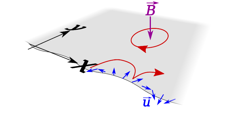
Figure 1: (Color online) A schematic picture of a continuous (graphene) sheet with an edge along the $x$-axis and an applied perpendicular magnetic field (purple). The electronic states (red) may be either localized Landau orbits in the bulk or dispersive states near the edge. Along the edge there are propagating acoustic (Rayleigh) edge waves given by a 2D displacement field (blue, amplitude exaggerated).

Since the graphene edge, which is normal to $-\bm{e}_{y}$ and located at $y=0$, is stress-free, the elastic boundary conditions are

$$\sigma_{jy}(x,0)=0,\;\;j=x,y,z\;,$$ (1)

where $\sigma_{ij}(x,y)$ is the usual 2D stress tensorLandau and Lifshitz (2008). Since the Rayleigh waves are pseudo-1D, they can be specified by the wave vector $x$-component $q$ alone, which will be referred to as the wave number. Standard techniquesLandau and Lifshitz (2008) give the two-component displacement field $\bm{u}^{(q)}(x,y)$ for an in-plane Rayleigh wave as

$$\bm{u}^{(q)}(x,y;t)=2u_{0}\begin{pmatrix}f^{(q)}_{x}(y)\cos(qx-\omega t)\\ \operatorname{sgn}(q)f^{(q)}_{y}(y)\sin(qx-\omega t)\end{pmatrix}\;,$$ (2)

where

$$\bm{f}^{(q)}_{x}(y)={e}^{-\lambda_{l}|q|y}-C_{x}{e}^{-\lambda_{t}|q|y}$$ (3)

and

$$\bm{f}^{(q)}_{y}(y)=-\lambda_{l}{e}^{-\lambda_{l}|q|y}+C_{y}{e}^{-\lambda_{t}|q|y}.$$ (4)

The dimensionless constants are

$$\lambda_{l}=0.81,\;\;\lambda_{t}=0.46,$$

$$C_{x}=0.61,\;\;C_{y}=1.3\;,$$ (5)

and depend only on the ratio of the transverse and longitudinal sound velocities in graphene, $s_{t}/s_{l}$, or, equivalently, on the Poisson ratio. The sound velocities are taken to be $s_{t}=1.4\cdot 10^{4}\text{ m/s}$ and $s_{l}=2.1\cdot 10^{4}\text{ m/s}$Castro et al. (2010); Kaasbjerg et al. (2012). The dispersion relation is linear,

$$\omega{(q)}=s_{R}|q|\;,$$ (6)

with Rayleigh-wave sound velocity $s_{R}=1.2\cdot 10^{4}\text{ m/s}$.

The electronic subsystem is described by the standard effective-model graphene Hamiltonian

$$\hat{\bm{H}}_{\text{el}}=v^{F}(\bm{\sigma}_{x}\hat{p_{x}}+\tau\bm{\sigma}_{y}\hat{p_{y}}),$$ (7)

where $v^{F}=1.0\cdot 10^{6}\text{ m/s}$ is the Fermi velocity of graphene, $\tau=+1$ ($-1$) for the $K$-point ($K^{\prime}$-point), the $\bm{\sigma}$s are the sublattice-space Pauli matricesCastro Neto et al. (2009); Nakada et al. (1996); Brey and Fertig (2006a) and the sublattice psuedospinor upon which the Hamiltonian acts is defined by $\bm{\psi}(x,y)=(\psi_{A}(x,y),\tau\psi_{B}(x,y))^{T}$. The transverse magnetic field is represented by a vector potential in the Landau gauge, $\bm{A}_{B}=(By,0)^{T}$, and then included in the Hamiltonian of Eq. (7) through the minimal coupling $\bm{p}\rightarrow\bm{p}+e\bm{A}$ (the electron charge is $-e<0$).

In an infinite bulk system the electronic energies form Landau levelsNovoselov et al. ; Jiang et al. (2007); Li et al. (2007),

$$E_{n} =\operatorname{sgn}(n)E_{1}\sqrt{|n|},\;\;n=0,\pm 1,\pm 2,\ldots$$

$$E_{1} =\sqrt{2}\hbar v^{F}l_{B}^{-1}\propto\sqrt{|B|}\;,$$ (8)

and the electronic wave functions are harmonic oscillator states centered around $y_{c}=-kl^{2}_{B}$, corresponding to closed Landau orbits, see Fig. 1. This simple picture is modified by the introduction of an edge.

In the considered system the edge at $y=0$ is a zigzag edge of $B$-atoms, leading to the electronic boundary conditionBrey and Fertig (2006b)

$$\psi_{A}(x,0)=0.$$ (9)

Since the zigzag boundary condition does not mix valleys the $K$- and $K^{\prime}$-points can be considered separately.

The edge induces a positive (negative) dispersion in the electron-like (hole-like) Landau levels as $k$ increases and the wave function center $y_{c}\propto-k$ moves toward and over the edgePeres et al. (2006), pressing the oscillator wave functions against the edge and turning them into edge-localized current-carrying states. For a classical, intuitive picture of this effect, see Fig. 1.

The dispersion can be calculated by generalizing the Landau-level index $n$ to a continuous analogue, $\nu=(E/E_{1})^{2}$, and the harmonic oscillator functions to (Whittaker’s) parabolic cylinder functions $D_{\nu}(z)$, which reduce to harmonic oscillator functions for integer $\nu$ but allow for non-integer $\nu$ solutions between the bulk Landau levels. The spectrum is then calculated from the boundary condition of Eq. (9)Gusynin et al. (2008a, b, 2009); Romanovsky et al. (2011). The dimensionless energy $E/E_{1}\equiv\tilde{E}$ is plotted against the dimensionless wave number $kl_{B}\equiv\tilde{k}$ in Fig. 2 for both the $K$- and $K^{\prime}$-points. The energy band stemming from Landau level $n$ will be referred to as “edge band $n$”. When $\tilde{k}=kl_{B}=0$, $y_{c}=0$ and the wave function is centered on the edge.

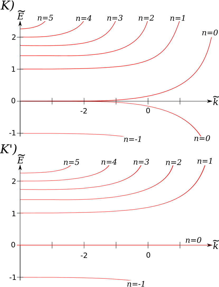
Figure 2: (Color online) A schematic picture of the electronic spectrum around the points $K$ (top) and $K^{\prime}$ (bottom). The scaled energy $\tilde{E}=E/E_{1}$ is plotted against the scaled wave number $\tilde{k}=kl_{B}$ (energy bands in red). The leftmost low-$\tilde{k}$ states are bulk states and their spectrum consists of discrete Landau levels. The dispersive states are edge states and here share the label $n$ with their bulk counterparts.

As seen in Fig. 2, the zeroth Landau level remains dispersonless for all $\tilde{k}$ in the $K^{\prime}$-point spectrum, whereas it is seemingly split in two edge bands, one electron-like and one hole-like, in the $K$-point spectrum. This can be explained by extra degeneracies introduced by topological edge states; the peculiar nature of the $n=0$ Landau level have been studied in other papersFujita et al. (1996); Arikawa et al. (2008); Gusynin et al. (2009); Romanovsky et al. (2011); for the purpose of this paper the schematic spectra in Fig. 2 will suffice.

The electronic pseudospinor wave functions are given in the appendix for reference. There, scaled physical coordinates $\tilde{x}(\tilde{y})\equiv x(y)/l_{B}$ are introduced, which will be employed below when considering the absorption.

The standard first-order-in-strain Hamiltonian for the electron-strain interaction in graphene is given by Suzuura and Ando (2002)

$$\bm{H}_{\text{int}}^{\tau}\left(\bm{u}(x,y;t)\right)=g_{1}(u_{xx}+u_{yy})\bm{I}+\\ +g_{2}\left(-\tau(u_{xx}-u_{yy})\bm{\sigma}_{x}+2u_{xy}\bm{\sigma}_{y}\right),$$ (10)

where $u_{i}j$ is the standard strain tensor. The diagonal elements are the scalar deformation potential, with coupling constant $g_{1}\sim 10\text{ eV}$, and the off-diagonal elements are usually imagined as a strain-induced pseudo vector-potential, and their coupling constant is $g_{2}\sim 1\text{ eV}$. Since the valley separation is $|\bm{K}-\bm{K}^{\prime}|\sim a^{-1}$, interaction with the acoustic Rayleigh waves will not mix $K$ and $K^{\prime}$ if the acoustic wave number $q\ll a^{-1}$, which must hold for the continuous-media model to be valid. Therefore all electronic transitions induced by the acoustic waves are intra-valley and the $K$- and $K^{\prime}$-point spectra can still be considered separately using $\tau=\pm 1$.

Inserting Eqs. (2), (3), and (4) into Eq. (10) yields the Hamiltonian for an electronic transition due to interaction with the acoustic Rayleigh waves as

$$\bm{H}_{\text{int}}^{\tau}\left(\bm{u}^{(q)}(x,y;t)\right)=u_{0}e^{iqx-i\omega t}(iq)\left\{g_{1}(T_{1}\bm{I}e^{-\lambda_{l}|q|y}+\right.\\ \left.+g_{2}\left(\left[-\tau T_{2}^{x,l}\bm{\sigma}_{x}+i\operatorname{sgn}(q)T_{2}^{y}\bm{\sigma}_{y}\right]e^{-\lambda_{l}|q|y}+\right.\right.\\ \left.\left.+\left[\tau T_{2}^{x,t}\bm{\sigma}_{x}-i\operatorname{sgn}(q)T_{2}^{y}\bm{\sigma}_{y}\right]e^{-\lambda_{t}|q|y}\right)\right\}+\text{H.c.}$$ (11)

where the constants are

$$T_{1}=0.34,\;\;T_{2}^{y}=1.6,$$

$$T_{2}^{x,l}=1.7,\;\;T_{2}^{x,t}=1.2\;.$$ (12)

Considering the spectra for the $K$- and $K^{\prime}$-points in Fig. 2, it is evident that using a gate voltage $V_{G}$ to adjust the scaled Fermi energy, $E^{F}/E_{1}=\tilde{E}^{F}\propto V_{G}/\sqrt{B}$, alters the number of dispersive energy bands crossing the Fermi level. If

$$|\tilde{E}_{n-1}|<|\tilde{E}^{F}|<|\tilde{E}_{n}|,$$ (13)

where $\tilde{E}_{n}$ refers to the scaled energy of bulk Landau level $n$ (see Eq. (8)), there will be $n$ ($n-1$) energy bands crossing the Fermi level in the $K$-spectrum ($K^{\prime}$-spectrum). These crossings are the quantized conduction channels of the quantum Hall effect theory and the absolute values in Eq. (13) correspond to the electron-hole symmetry of the spectrum. The dispersionless level in the $K^{\prime}$-spectrum never crosses the Fermi level and is therefore assumed never to be involved in transitions.

To analyze the possible transitions, consider the transition rate between levels, thereby introducing conservation laws. The transition rate $W_{m,n}$ for an electronic jump from energy band $n$ to energy band $m$ due to interaction with an acoustic wave with scaled wave number $ql_{B}\equiv\tilde{q}$ is given by the Fermi golden rule,

$$W_{m,n}=\frac{2\pi}{\hbar}\sum_{\tilde{k}_{n}}\int\operatorname{d}\!{\tilde{E}_{m}}\delta\left(\tilde{E}_{n}+\tilde{E_{R}}-\tilde{E}_{m}\right)\delta_{\tilde{k}_{n}+\tilde{q},\tilde{k}_{m}}\times\\ \times\rho(E_{m})\left|\Lambda_{\tilde{k}_{m};\tilde{q};\tilde{k}_{n}}^{\tau}\right|^{2}f_{\text{FD}}(E_{n})\left(1-f_{\text{FD}}(E_{m})\right).$$ (14)

Here, $\delta_{\tilde{k}_{n}+\tilde{q},\tilde{k}_{m}}\Lambda_{\tilde{k}_{m};q;\tilde{k}_{n}}^{\tau}$ is the matrix element of an induced transition from $\tilde{k}_{n}$ to $\tilde{k}_{m}$ defined by

$$\delta_{\tilde{k}_{n}+\tilde{q},\tilde{k}_{m}}\Lambda_{\tilde{k}_{m};\tilde{q};\tilde{k}_{n}}^{\tau}=\\ l_{B}^{2}\iint_{\mathit{S}}\bm{\psi}^{\tau,\tilde{k}_{m}\dagger}_{\nu}\bm{H}_{\text{int}}^{\tau}\left(\bm{u}^{(q)}\right)\bm{\psi}^{\tau,\tilde{k}_{n}}_{\nu}\operatorname{d}\!{\tilde{x}}d{\tilde{y}}$$ (15)

where the interaction is given by Eq. (11) (the harmonic time dependence is accounted for by the energy conservation), the electronic wave functions are given in the appendix and the integration surface is the whole sheet $\mathit{S}$ in terms of the scaled coordinates. The continuous level index is $\nu=(E/E_{1})^{2}$ as before, $f_{\text{FD}}(E(k))$ is the Fermi-Dirac distribution function, $\rho(E_{m})$ is the density of final states, $\tilde{k}_{n}$ is the scaled wave number for an electronic state in energy band $n$ corresponding to energy $\tilde{E}_{n}$, and the scaled acoustic dispersion is given by, using Eq. (6),

$$\tilde{E}_{R}\left(\tilde{q}\right)=\tilde{s}_{R}|\tilde{q}|\;,$$ (16)

with dimensionless speed of sound

$$\tilde{s}_{R}\equiv\frac{s_{R}}{\sqrt{2}v^{F}}\;.$$ (17)

The energy integration and the Fermi-Dirac factors confine the energy region of absorption to the vicinity of the Fermi energy, $E_{n}\lesssim E^{F}\lesssim E_{m}$, and thus imply that the energies and wave numbers may be taken at the Fermi level, e.g. $\tilde{k}_{n}\rightarrow\tilde{k}^{F}_{n}$. Armed with this knowledge, the picture can be simplified by linearizing the spectrum, swapping each curved energy band $n$ for a linear band $n$ with velocity equal to the Fermi velocity $v_{n}$ of the band, see Fig. 3. Then the linearized dimensionless dispersion of band $n$ is

$$\tilde{E}_{n}\left(\tilde{k}_{n}\right)=\tilde{v}_{n}\left(\tilde{k}_{n}-\tilde{k}^{F}_{n}\right)+\tilde{E}^{F}$$ (18)

where the dimensionless velocity of the band is defined analogously to Eq. (17),

$$\tilde{v}_{n}\equiv\frac{v_{n}}{\sqrt{2}v^{F}},$$ (19)

and $\tilde{s}_{R}\ll\tilde{v}_{n}\forall n$.

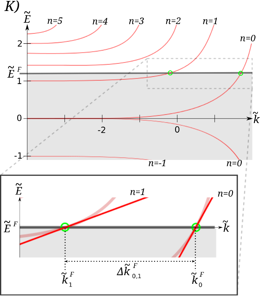
Figure 3: (Color online) In the $K$-point spectrum of Fig. 2 the Fermi energy $\tilde{E}^{F}$ (horizontal grey line) is set by a gate voltage to lie between, say, bulk Landau level 1 and Landau level 2, thus giving the spectrum two Fermi crossing points (green circles), at $\tilde{k}^{F}_{1}$ and $\tilde{k}^{F}_{0}$, for energy band $1$ and $0$ respectively. Since transitions occur only near the Fermi level, the spectrum can be linearized, resulting in an effective model with two linear bands crossing the Fermi level at points $\tilde{k}^{F}_{1}$ and $\tilde{k}^{F}_{0}$ (see magnified inset). The resonant frequency is then given by the wave number separation at the Fermi level $\Delta\tilde{k}^{F}_{0,1}=|\tilde{k}^{F}_{0}-\tilde{k}^{F}_{1}|$. The picture is schematic.

.

The above arguments together with energy and momentum conservation restrict the number of allowed transitions by imposing the requirement that

$$\tilde{q}\approx\tilde{k}^{F}_{m}-\tilde{k}^{F}_{n}\equiv\Delta\tilde{k}^{F}_{m,n},$$ (20)

i.e. the acoustic wave number $\tilde{q}$ must roughly match the $\tilde{k}$-separation of the two Fermi crossing points. Transitions occur in the vicinity of the Fermi level, not at the Fermi level, but for the purpose of this paper it is sufficient to take $\tilde{q}=\Delta\tilde{k}^{F}_{m,n}$. The same above arguments also imply that there are no allowed intra-level transitions, $n\neq m$.

The number of band-to-band transitions $N_{t}(n)$ for $n$ Fermi level crossings is then

$$N_{t}\left(n\right)=\begin{cases}\frac{n!}{2(n-2)!}&\mbox{if }n\geq 2,\\ 0&\mbox{if }n<2\;,\end{cases}$$ (21)

and it must be remembered that transitions can occur in both the $K$- and $K^{\prime}$-spectra.

Since the spacing $\Delta\tilde{k}^{F}_{n+1,n}$ between neighboring Fermi crossings is approximately equal for the same energy, i.e. $\Delta\tilde{k}^{F}_{n,n+j}\approx j\cdot\Delta\tilde{k}^{F}_{m,m+1}$, it is potentially useful to group the transitions in terms of how many bands they jump, i.e. a jump from band $n$ to band $n-j$ is a $j$-jump (the minus sign is due to Fermi crossings of higher-$n$ bands having larger $\tilde{k}$). For the situation with $n$ Fermi crossings in one of the valley spectra, the number of $j$-jumps is

$$N_{t,j}\left(n\right)=\begin{cases}n-j&\mbox{if }n>2,\\ 0&\mbox{if }n\leq 2.\end{cases}$$ (22)

Summing $N_{t,j}$ for all $j<n$ yields the total number of transitions in the spectrum, $N_{t}$. Since all $j$-jumps have approximately equal $\Delta\tilde{k}^{F}_{m,n}$, i.e. absorbed acoustic frequency, they might appear as a multi-peak in the absorption spectrum: $N_{t,j}$ peaks close together.

The absorbed acoustic frequencies $sl_{B}^{-1}\Delta\tilde{k}^{F}_{m,n}$ can be found by using the electronic boundary conditions to find the Fermi level crossings $\tilde{k}^{F}_{n}$, see the appendix. These frequencies are on the order of $sl_{B}^{-1}\sim\sqrt{B[T]}\cdot 10^{11}\text{s}^{-1}$ and depend only on the scaled Fermi energy $\tilde{E_{F}}$, i.e. the relative position of the Fermi level. The periods of these acoustic frequencies must be much shorter than the acoustic decay time due to interaction with the electronic subsystem for the Fermi golden rule to remain valid.

For the linearized spectrum, Eq. (18), standard periodic boundary conditions in the $x$-direction yields the density of final states per unit length $\rho(E_{m})$ as

$$\rho(E_{m})=\frac{1}{2\sqrt{2}\pi\hbar v^{F}\tilde{v}_{m}}.$$ (23)

As seen in Fig. 2, the density of states increases with edge localization, i.e. increasing $\tilde{k}$.

Since transitions occur near the Fermi level, the matrix element of transition in Eq. (15) is evaluated for $\tilde{q}=\Delta\tilde{k}_{m,n}$ and $\tilde{E}_{n}=\tilde{E}_{m}=\tilde{E}^{F}$, and is then

$$\Lambda_{\tilde{k}^{F}_{m};\tilde{k}^{F}_{n}}^{\tau}=i\Delta\tilde{k}^{F}_{m,n}\left(\frac{u_{0}}{l_{B}}\right)\left(g_{1}F_{1}+g_{2}F_{2}\right)$$ (24)

where the dimensionless transition-dependent integrals have been separated into a scalar potential contribution $F_{1}$ and pseudo-magnetic-field contribution $F_{2}$; both given in the appendix. Normalization of the electronic wave functions causes these integrals to be at the most unity.

Inserting the above into Eq. (14), the final expression for the absorption rate per unit length is

$$W_{m,n}=\\ \left(\frac{1}{\sqrt{2}\hbar^{2}v^{F}}\right)\frac{\left(\Delta\tilde{k}^{F}_{m,n}\right)^{2}}{\tilde{v}_{m}}\left(\frac{u_{0}}{l_{B}}\right)^{2}\left|g_{1}F_{1}+g_{2}F_{2}\right|^{2}.$$ (25)

where all relevant depencies have been included explicitly for clarity. The first factor $\approx 1.6\cdot 10^{24}\text{eV}^{-2}\text{s}^{-1}\text{m}^{-1}$ and consists of general constants, and the second factor constists of parameters specific to the transition in question and is $\sim 2$. The third is the amplitude dependence, with the amplitude scaled by the magnetic length. By assumptiom, the amplitude is low, $A\ll l_{b}$, causing this factor to be very small. The final factor is the coupling coefficients and the transition integrals, which are less than one by normalization, meaning that the order of magnitude is set by the coupling. Inserting the definition of the magnetic length yields $W_{m,n}\propto B$. This direct proportionality to the field comes from the $iq$-factor in the strain tensor and the fact that absorption occurs only for the phonon wave numbers $q$ which match the electro-magnetic spectrum and are thus are on the order of inverse magnetic length.

The total energy of the acoustic wave isEzawa (1971)

$$E_{\text{ac}}=\rho_{\text{gr}}\omega(q)^{2}\iint_{\mathit{S}}|\bm{u}^{(q)}(x,y;0)|^{2}\operatorname{d}\!{x}d{y}$$ (26)

where $\rho_{\text{gr}}=7.6\cdot 10^{-7}\text{kg}/\text{m}^{2}$ is the surface mass density of grapheneKaasbjerg et al. (2012). In this case

$$\iint_{\mathit{S}}|\bm{u}^{(q)}(x,y;0)|^{2}\operatorname{d}\!{x}d{y}=\frac{2Lu_{0}^{2}}{|q|N_{\text{ac}}^{2}}\;,$$ (27)

and it can be shown that

$$N_{\text{ac}}=1.2,$$ (28)

whereas the energy lost to each electronic transition is simply $\hbar\omega(q)$. The acoustic inverse decay time $\tau_{D}$ due to interaction with the electronic subsystem is then given by

$$\frac{1}{\tau_{D}} =\left(\frac{N_{\text{ac}}^{2}\left(\Delta\tilde{k}^{F}_{m,n}\right)^{2}}{2\sqrt{2}\hbar v^{F}\tilde{v}_{m}\rho_{\text{gr}}l_{B}^{2}s_{R}}\right)\left|g_{1}F_{1}+g_{2}F_{2}\right|^{2}$$

$$=\frac{2.0\cdot 10^{7}B[T]}{\text{s eV}^{2}}\frac{\left(\Delta\tilde{k}^{F}_{m,n}\right)^{2}}{\tilde{v}_{m}}\left|g_{1}F_{1}+g_{2}F_{2}\right|^{2}.$$ (29)

As an example, consider the simplest case. The gate voltage is adjusted in relation the magnetic field so that

$$\tilde{E}^{F}=\frac{\tilde{E}_{1}+\tilde{E}_{2}}{2},$$ (30)

i.e. the Fermi level is now in the middle of the gap between Landau level 1 and 2. According to Eq. (13) there will be $2$ bands crossing the Fermi level in the $K$-point spectrum ($1$ in the $K^{\prime}$-spectrum) and by Eq. (21) there will, trivially, be $1$ possible transition ($0$ possible transitions). Eq. (22) specifies that this one transition will be between neighboring levels. Solving Eq. (35) numerically returns $\tilde{k}^{F}_{1}=-1.29$ and $\tilde{k}^{F}_{0}=0.36$, the points where the bands intersect the Fermi level. This leads to $\Delta\tilde{k}^{F}_{0,1}=1.65$, which will be the acoustic wave number absorbed in the transition from edge band $1$ to edge band $0$. The set $\tilde{E}^{F}$ means that the generalized level index is, according to Eq. (37), $\nu^{F}=((1+\sqrt{2})/2)^{2}\approx 1.4571$ and the velocity of the destination band is estimated to $\tilde{v}_{0}\approx 0.6$ (in general, $\tilde{v}_{0}\sim 0.5$). Using the wave functions of Eq. (33) with parameters $\nu^{F}$ and $\tilde{k}^{F}_{1}$ ($\tilde{k}^{F}_{0}$) for edge band $1$ ($0$) as well as the acoustic wave number $\Delta\tilde{k}^{F}_{0,1}$ allows for numerical evaluation of the integrals in the appendix. The interaction integrals in Eqs. (38) and (39) yield $F_{1}=-0.0546$ and $F^{\tau}_{2}=-0.0918$. Inserting all known values into Eq (29) the resulting inverse decay time is

$$\frac{1}{\tau_{D}}=\frac{9.1\cdot 10^{7}B[T]}{\text{s eV}^{2}}\left|0.0546g_{1}+0.0918g_{2}\right|^{2}.$$ (31)

With the standard valuesSuzuura and Ando (2002) of $g_{1}\approx 20\text{ eV}$ and $g_{2}\approx 2\text{ eV}$, the decay time becomes $\tau_{D}\approx 6.8\text{ ns}/B[T]$, which corresponds to a characteristic decay length of $82\text{ }\mu\text{m}/B[T]$. The decay time is much longer than the acoustic period $\sim\sqrt{B[T]}10^{-11}\text{ s}$, thus validating our use of the Fermi golden rule.

In conclusion, we have shown that a stress-free graphene edge supports propagating vibrational in-plane edge modes in the form of 2D Rayleigh waves, and that interaction with such waves can cause electronic transitions between the electronic edge states induced by a perpendicular magnetic field.

Since momentum conservation requires the wavelength of the acoustic waves to be on scale of the magnetic length for transitions to occur, the magnetic field strength enters into the low-amplitude absorption rate as a simple proportionality through the strain tensor.

With the expressions given in this paper, both the absorbed acoustic frequencies and the resulting decay time can be calculated for all electronic transitions of the considered type, yielding an acoustic absorption spectrum which could be used for result confirmation in a wave-propagation experiment.

We suggest, based on comparison with similar systemsBorovik et al. (1989), that this edge-localized interaction could result in nonlinear phenomena such as acoustic solitons propagating along the edge.

I Acknowledgements

We thank L. Gorelik for valuable discussion, E. Cojocaru for his Matlab scriptsCojocaru (2009) and the Swedish Research Council (VR) for funding.

Appendix A Electronic wave functions

The electronic pseudospinor wave functions of the energy band $n$ and $m$, areGusynin et al. [2008a, b, 2009], Romanovsky et al. [2011]

$$\bm{\psi}_{\nu}^{\tau,\tilde{k}}(x,y)=\frac{N^{\tau,k}_{\nu}}{\sqrt{Ll_{B}}}{e}^{i\tilde{k}\tilde{x}}\bm{\phi}^{\tau,\tilde{k}}_{\nu}(\tilde{y}),$$ (32)

where $\tau$ labels the valley ($K$ or $K^{\prime}$) as before. The $y$-dependent factor is

$$\bm{\phi}^{+1,\tilde{k}}_{\nu}(\tilde{y})=\begin{pmatrix}D_{\nu}(\sqrt{2}(\tilde{k}+\tilde{y}))\\ \sqrt{\nu}D_{\nu-1}(\sqrt{2}(\tilde{k}+\tilde{y}))\end{pmatrix},$$ (33)

for the $K$-point and

$$\bm{\phi}^{-1,\tilde{k}}_{\nu}(\tilde{y})=\begin{pmatrix}\sqrt{\nu}D_{\nu-1}(\sqrt{2}(\tilde{k}+\tilde{y}))\\ -D_{\nu}(\sqrt{2}(\tilde{k}+\tilde{y}))\end{pmatrix},$$ (34)

for the $K^{\prime}$-point. The factors $N_{\tau,n,k}/(\sqrt{Ll_{B}})$ are normalization constants.

Appendix B Fermi level crossings

The edge boundary condition of Eq. (9) ultimately gives an equation for the electronic spectrum. At the Fermi energy $E_{F}$ this equation reads, for the $K$-point,

$$D_{{\nu}^{F}}\left(\sqrt{2}\tilde{k}^{F}\right)=0,$$ (35)

and for the $K^{\prime}$-point

$$D_{{\nu}^{F}-1}\left(\sqrt{2}\tilde{k}^{F}\right)=0,$$ (36)

where

$${\nu}^{F}=\left(\tilde{E}^{F}\right)^{2}.$$ (37)

Solving Eqs. (35) and (36) for $\tilde{k}^{F}$ gives the Fermi crossing points $\tilde{k}^{F}_{n}$ for the given $\tilde{E}^{F}$. Identifying them with the different bands allows for calculation of $\Delta\tilde{k}^{F}_{m,n}$ and thus the absorbed acoustic frequencies. In general $\Delta\tilde{k}^{F}_{m,n}\sim 1$.

Appendix C Absorption integrals

Here the dimensionless transition integrals that enter into the transition matrix element are given. Since the integrands decay into the bulk, they are easily evaluated using a cutoff. The integral giving the scalar-potential contribution to the absorption is (normalization constants have been moved to the left hand side for brevity)

$$\frac{F_{1}}{N^{\tau,k^{F}_{m}*}_{\nu^{F}}N^{\tau,k^{F}_{n}}_{\nu^{F}}}=\\ T_{1}\int_{0}^{\infty}\bm{\phi}^{\tau,\tilde{k}^{F}_{m}\dagger}_{{\nu}^{F}}(\tilde{y})\bm{\phi}^{\tau,\tilde{k}^{F}_{n}}_{{\nu}^{F}}(\tilde{y})e^{-\lambda_{l}|\Delta\tilde{k}^{F}_{m,n}|\tilde{y}}d{\tilde{y}},$$ (38)

and the pseudo-magnetic-field contribution integral is

$$\frac{F_{2}}{N^{\tau,k^{F}_{m}*}_{\nu^{F}}N^{\tau,k^{F}_{n}}_{\nu^{F}}}=\tau\int_{0}^{\infty}\bm{\phi}^{\tau,\tilde{k}^{F}_{m}\dagger}_{{\nu}^{F}}(\tilde{y})\bm{\sigma}_{x}\bm{\phi}^{\tau,\tilde{k}^{F}_{n}}_{{\nu}^{F}}(\tilde{y})\times\\ \left(-T^{x,l}_{2}e^{-\lambda_{l}\Delta|\tilde{k}^{F}_{m,n}|\tilde{y}}+T^{x,t}_{2}e^{-\lambda_{t}|\Delta\tilde{k}^{F}_{m,n}|\tilde{y}}\right)d{\tilde{y}}+\\ i\operatorname{sgn}(\Delta\tilde{k}^{F}_{m,n})T^{y}_{2}\int_{0}^{\infty}\bm{\phi}^{\tau,\tilde{k}^{F}_{m}\dagger}_{{\nu}^{F}}(\tilde{y})\bm{\sigma}_{y}\bm{\phi}^{\tau,\tilde{k}^{F}_{n}}_{{\nu}^{F}}(\tilde{y})\times\\ \left(e^{-\lambda_{l}\Delta|\tilde{k}^{F}_{m,n}|\tilde{y}}-e^{-\lambda_{t}|\Delta\tilde{k}^{F}_{m,n}|\tilde{y}}\right)d{\tilde{y}}.$$ (39)

The numerical normalization constants are given by

$$\left|N^{\tau,k^{F}_{n}}_{\nu^{F}}\right|^{2}=\frac{1}{\int_{0}^{\infty}\left|\bm{\phi}^{\tau,\tilde{k}^{F}_{n}}_{{\nu}^{F}}(\tilde{y})\right|^{2}d{\tilde{y}}}.$$ (40)

References

- Novoselov et al. (2004) K. S. Novoselov, A. K. Geim, S. V. Morozov, D. Jiang, Y. Zhang, S. V. Dubonos, I. V. Grigorieva, and A. A. Firsov. Electric field effect in atomically thin carbon films. Science, 306(5696):666–669, 2004. doi: 10.1126/science.1102896. URL http://www.sciencemag.org/content/306/5696/666.abstract.
- Geim and Novoselov (2007) A. K. Geim and K. S. Novoselov. The rise of graphene. Nat. mater., 6:183–191, March 2007. doi: 10.1038/nmat1849. URL http://www.nature.com/nmat/journal/v6/n3/full/nmat1849.html.
- Landau and Lifshitz (2008) L. D. Landau and E. M. Lifshitz. Theory of Elasticity. Butterworth-Heinemann, 2008.
- Heil et al. (1984) J Heil, I Kouroudis, B Luthi, and P Thalmeier. Surface acoustic waves in metals. Journal of Physics C: Solid State Physics, 17(13):2433, 1984. URL http://stacks.iop.org/0022-3719/17/i=13/a=024.
- Willett et al. (1990) R. L. Willett, M. A. Paalanen, R. R. Ruel, K. W. West, L. N. Pfeiffer, and D. J. Bishop. Anomalous sound propagation at =1/2 in a 2d electron gas: Observation of a spontaneously broken translational symmetry? Phys. Rev. Lett., 65:112–115, Jul 1990. doi: 10.1103/PhysRevLett.65.112. URL http://link.aps.org/doi/10.1103/PhysRevLett.65.112.
- Willett et al. (1993) R. L. Willett, R. R. Ruel, M. A. Paalanen, K. W. West, and L. N. Pfeiffer. Enhanced finite-wave-vector conductivity at multiple even-denominator filling factors in two-dimensional electron systems. Phys. Rev. B, 47:7344–7347, Mar 1993. doi: 10.1103/PhysRevB.47.7344. URL http://link.aps.org/doi/10.1103/PhysRevB.47.7344.
- Thalmeier (2011) Peter Thalmeier. Surface phonon propagation in topological insulators. Phys. Rev. B, 83:125314, Mar 2011. doi: 10.1103/PhysRevB.83.125314. URL http://link.aps.org/doi/10.1103/PhysRevB.83.125314.
- Simon (1996) Steven H. Simon. Coupling of surface acoustic waves to a two-dimensional electron gas. Phys. Rev. B, 54:13878–13884, Nov 1996. doi: 10.1103/PhysRevB.54.13878. URL http://link.aps.org/doi/10.1103/PhysRevB.54.13878.
- Thalmeier et al. (2010) Peter Thalmeier, Balázs Dóra, and Klaus Ziegler. Surface acoustic wave propagation in graphene. Phys. Rev. B, 81:041409, Jan 2010. doi: 10.1103/PhysRevB.81.041409. URL http://link.aps.org/doi/10.1103/PhysRevB.81.041409.
- Savin and Kivshar (2010) Alexander V. Savin and Yuri S. Kivshar. Vibrational tamm states at the edges of graphene nanoribbons. Phys. Rev. B, 81:165418, Apr 2010. doi: 10.1103/PhysRevB.81.165418. URL http://link.aps.org/doi/10.1103/PhysRevB.81.165418.
- Peres et al. (2006) N. M. R. Peres, F. Guinea, and A. H. Castro Neto. Electronic properties of disordered two-dimensional carbon. Phys. Rev. B, 73:125411, Mar 2006. doi: 10.1103/PhysRevB.73.125411. URL http://link.aps.org/doi/10.1103/PhysRevB.73.125411.
- Gusynin et al. (2008a) V. P. Gusynin, V. A. Miransky, S. G. Sharapov, and I. A. Shovkovy. Edge states in quantum hall effect in graphene (review article). Low Temperature Physics, 34(10):778–789, 2008a. doi: 10.1063/1.2981387. URL http://link.aip.org/link/?LTP/34/778/1.
- Gusynin et al. (2008b) V. P. Gusynin, V. A. Miransky, S. G. Sharapov, and I. A. Shovkovy. Edge states, mass and spin gaps, and quantum hall effect in graphene. Phys. Rev. B, 77:205409, May 2008b. doi: 10.1103/PhysRevB.77.205409. URL http://link.aps.org/doi/10.1103/PhysRevB.77.205409.
- Gusynin et al. (2009) V. P. Gusynin, V. A. Miransky, S. G. Sharapov, I. A. Shovkovy, and C. M. Wyenberg. Edge states on graphene ribbons in magnetic field: Interplay between dirac and ferromagnetic-like gaps. Phys. Rev. B, 79:115431, Mar 2009. doi: 10.1103/PhysRevB.79.115431. URL http://link.aps.org/doi/10.1103/PhysRevB.79.115431.
- Romanovsky et al. (2011) Igor Romanovsky, Constantine Yannouleas, and Uzi Landman. Unique nature of the lowest landau level in finite graphene samples with zigzag edges: Dirac electrons with mixed bulk-edge character. Phys. Rev. B, 83:045421, Jan 2011. doi: 10.1103/PhysRevB.83.045421. URL http://link.aps.org/doi/10.1103/PhysRevB.83.045421.
- Castro Neto et al. (2009) A. H. Castro Neto, F. Guinea, N. M. R. Peres, K. S. Novoselov, and A. K. Geim. The electronic properties of graphene. Rev. Mod. Phys., 81:109–162, Jan 2009. doi: 10.1103/RevModPhys.81.109. URL http://link.aps.org/doi/10.1103/RevModPhys.81.109.
- Brey and Fertig (2006a) Luis Brey and H. A. Fertig. Edge states and the quantized hall effect in graphene. Phys. Rev. B, 73:195408, May 2006a. doi: 10.1103/PhysRevB.73.195408. URL http://link.aps.org/doi/10.1103/PhysRevB.73.195408.
- Castro et al. (2010) Eduardo V. Castro, H. Ochoa, M. I. Katsnelson, R. V. Gorbachev, D. C. Elias, K. S. Novoselov, A. K. Geim, and F. Guinea. Limits on charge carrier mobility in suspended graphene due to flexural phonons. Phys. Rev. Lett., 105:266601, Dec 2010. doi: 10.1103/PhysRevLett.105.266601. URL http://link.aps.org/doi/10.1103/PhysRevLett.105.266601.
- Kaasbjerg et al. (2012) Kristen Kaasbjerg, Kristian S. Thygesen, and Karsten W. Jacobsen. Unraveling the acoustic electron-phonon interaction in graphene. Phys. Rev. B, 85:165440, Apr 2012. doi: 10.1103/PhysRevB.85.165440. URL http://link.aps.org/doi/10.1103/PhysRevB.85.165440.
- Nakada et al. (1996) Kyoko Nakada, Mitsutaka Fujita, Gene Dresselhaus, and Mildred S. Dresselhaus. Edge state in graphene ribbons: Nanometer size effect and edge shape dependence. Phys. Rev. B, 54:17954–17961, Dec 1996. doi: 10.1103/PhysRevB.54.17954. URL http://link.aps.org/doi/10.1103/PhysRevB.54.17954.
- (21) K. S. Novoselov, A. K. Geim, S. V. Morozov, D. Jiang, M. I. Katsnelson, I. V. Grigorieva, and S. V. Dubonos. Two-dimensional gas of massless dirac fermions in graphene.
- Jiang et al. (2007) Z. Jiang, E. A. Henriksen, L. C. Tung, Y.-J. Wang, M. E. Schwartz, M. Y. Han, P. Kim, and H. L. Stormer. Infrared spectroscopy of landau levels of graphene. Phys. Rev. Lett., 98:197403, May 2007. doi: 10.1103/PhysRevLett.98.197403. URL http://link.aps.org/doi/10.1103/PhysRevLett.98.197403.
- Li et al. (2007) Guohong Li, Eva Y. Andrei, and A. A. Firsov. Observation of landau levels of dirac fermions in graphite. Nat Phys, 3:623, September 2007. doi: 10.1038/nphys653. URL http://www.nature.com/nphys/journal/v3/n9/suppinfo/nphys653_S1.html.
- Brey and Fertig (2006b) L. Brey and H. A. Fertig. Electronic states of graphene nanoribbons studied with the dirac equation. Phys. Rev. B, 73:235411, Jun 2006b. doi: 10.1103/PhysRevB.73.235411. URL http://link.aps.org/doi/10.1103/PhysRevB.73.235411.
- Fujita et al. (1996) Mitsutaka Fujita, Katsunori Wakabayashi, Kyoko Nakada, and Koichi Kusakabe. Peculiar localized state at zigzag graphite edge. Journal of the Physical Society of Japan, 65(7):1920–1923, 1996. doi: 10.1143/JPSJ.65.1920. URL http://dx.doi.org/10.1143/JPSJ.65.1920.
- Arikawa et al. (2008) Mitsuhiro Arikawa, Yasuhiro Hatsugai, and Hideo Aoki. Edge states in graphene in magnetic fields: A specialty of the edge mode embedded in the n=0 landau band. Phys. Rev. B, 78:205401, Nov 2008. doi: 10.1103/PhysRevB.78.205401. URL http://link.aps.org/doi/10.1103/PhysRevB.78.205401.
- Suzuura and Ando (2002) Hidekatsu Suzuura and Tsuneya Ando. Phonons and electron-phonon scattering in carbon nanotubes. Phys. Rev. B, 65:235412, May 2002. doi: 10.1103/PhysRevB.65.235412. URL http://link.aps.org/doi/10.1103/PhysRevB.65.235412.
- Ezawa (1971) Hiroshi Ezawa. Phonons in a half space. Ann. Phys., 67:438–460, 1971.
- Borovik et al. (1989) A. E. Borovik, E. N. Bratus, and V. S. Shumeiko. Hypersonic solitons in metals. Sov. Phys. JETP, 68:826–832, April 1989.
- Cojocaru (2009) E. Cojocaru. Parabolic cylinder functions implemented in matlab. January 2009. URL arXiv:0901.2220.