The antikick strikes back: recoil velocities for nearly-extremal
binary black hole mergers in the test-mass limit

Abstract

Gravitational waves emitted from a generic binary black-hole merger carry away linear momentum anisotropically, resulting in a gravitational recoil, or “kick”, of the center of mass. For certain merger configurations the time evolution of the magnitude of the kick velocity has a local maximum followed by a sudden drop. Perturbative studies of this “antikick” in a limited range of black hole spins have found that the antikick decreases for retrograde orbits as a function of negative spin. We analyze this problem using a recently developed code to evolve gravitational perturbations from a point-particle in Kerr spacetime driven by an effective-one-body resummed radiation reaction force at linear order in the mass ratio $\nu\ll 1$. Extending previous studies to nearly-extremal negative spins, we find that the well-known decrease of the antikick is overturned and, instead of approaching zero, the antikick increases again to reach $\Delta v/(c\nu^{2})=3.37\times 10^{-3}$ for dimensionless spin ${\hat{a}}=-0.9999$. The corresponding final kick velocity is $v_{end}/(c\nu^{2})=0.076$. This result is connected to the nonadiabatic character of the emission of linear momentum during the plunge. We interpret it analytically by means of the quality factor of the flux to capture quantitatively the main properties of the kick velocity. The use of such quality factor does not require trajectories nor horizon curvature distributions and should therefore be useful both in perturbation theory and numerical relativity.

I Introduction

The anisotropic emission of gravitational radiation in coalescing black hole binaries carries away linear momentum from the system, which results in a net recoil of the center of mass. This gravitational recoil, or “kick”, can be related to a delicate and complicated interference between the gravitational wave (GW) multipoles. In the test-mass limit the recoil can be computed using perturbative methods by modeling the small black hole as a point-particle. Perturbative studies are crucial to study the basic features of the interference pattern among different multipoles. A detailed understanding of the recoil in the perturbative regime is important not only for binaries with an extreme mass ratio, but also for comparable masses. As pointed out in Ref. Nagar (2013) extrapolation from the test-mass result delivers quantitative agreement with numerical relativity for non-rotating black holes. Furthermore, for a rotating central black hole only the perturbative framework can systematically probe the extremal regime.

Recoil computations in the test-mass limit were performed recently by two groups using time domain calculations. The case with a non-rotating central black hole was studied in Bernuzzi and Nagar (2010) solving the Regge-Wheeler-Zerilli (RWZ) equations for gravitational metric perturbations. The case with a rotating central black hole was studied in Sundararajan et al. (2010) (SKH hereafter) solving the Teukolsky equation for gravitational curvature perturbations. The SKH analysis was limited to spin magnitudes $|{\hat{a}}|\leq 0.9$, where ${\hat{a}}$ is the dimensionless angular momentum parameter. In particular, SKH studied the drop in the time evolution of the recoil velocity, or “antikick” Baker et al. (2006); Schnittman et al. (2008), as a function of spin, and found that it is “essentially non-existent” for large spin retrograde coalescences.

Building on recent progress in solving numerically the Teukolsky equation with a point-particle source in the time domain Harms et al. (2014), we revisit the SKH analysis and extend it to nearly-extremal spin values, particularly focusing on the retrograde case with spin parameters up to ${\hat{a}}=-0.9999$. The extension of the parameter space reveals a new phenomenon: the antikick significantly reappears for $-1<{\hat{a}}<-0.9$. We explain this phenomenon by analyzing and relating the dynamics of the plunge and the GW linear momentum flux. As noted long ago by Damour and Gopakumar Damour and Gopakumar (2006) (DG hereafter) the time-evolution of the recoil velocity (also for the comparable mass ratio case) and, in particular, the existence of an antikick can be directly connected to the nonadiabatic emission of linear momentum during the plunge. Following DG, the behavior of the antikick as a function of ${\hat{a}}$ is understood analytically and quantified in a “quality factor” $Q$ associated to the maximum of the GW linear momentum flux (Sec. IV). This understanding of the antikick relies on gauge-invariant notions and may be a useful alternative to previous discussions that emphasize the trajectory Price et al. (2011, 2013) or curvature distributions on the horizon Rezzolla et al. (2010).

To set the stage for our analysis, we discuss the dynamics of the system providing a quantitative measure for its nonadiabaticity (Sec. II), and point out interesting properties of the GW linear momentum flux (Sec. III): as ${\hat{a}}\to-1$, the linear momentum flux shows a characteristic, multi-peaked interference pattern that can be explained by the increased importance of the subdominant waveform multipoles $0\leq m<\ell$ during the plunge Harms et al. (2014). The behavior of the maximal and final recoil velocity is discussed and analytically explained in Sec. IV. We examine the accuracy of our results in the Appendix, including extremal positive spins, $+0.9\leq{\hat{a}}\leq+0.9999$, that require special care.

We use geometric units $c=G=1$. The dynamics of the particle is obtained using a Hamiltonian formulation Harms et al. (2014); Damour and Nagar (2014) and expressed in dimensionless canonical variables.

II Dynamics: measuring nonadiabaticity

In the test-mass limit we model the black-hole binary system by a central spinning black hole of mass $M$ and a nonspinning particle of mass $\mu$, such that $\nu=\mu/M\ll 1$. Our test-mass calculations follow the method developed in Nagar et al. (2007); Bernuzzi and Nagar (2010), extended to the Kerr background in Harms et al. (2014). The gravitational waveforms used to compute the flux of linear momentum are extracted at future null infinity with a perturbative method based on the solution of the Teukolsky equation in the time domain. The black hole spin is either aligned or anti-aligned with the orbital angular momentum. The relative dynamics is driven by an effective-one-body resummed analytic radiation reaction Damour et al. (2009); Pan et al. (2011) at linear order in $\nu$. For simplicity, we do not include horizon absorption Nagar and Akcay (2012); Taracchini et al. (2013), so that the radiation reaction only incorporates the angular momentum flux emitted to infinity, following Harms et al. (2014). Since our radiation reaction is certainly inaccurate as ${\hat{a}}\to 1$ (because of both the absence of horizon absorption and the lack of higher-order spin-dependent terms in the resummed flux at infinity Harms et al. (2014); Taracchini et al. (2014)) our results for large, positive spin may be partly affected by systematic uncertainties. For this reason, we discuss in the main text only the spin range $-0.9999\leq{\hat{a}}\leq+0.9$, while the more challenging regime $+0.9<{\hat{a}}\leq+0.9999$ is discussed separately in Appendix A. Our main new findings are in the regime ${\hat{a}}\to-1$, where the analytic radiation reaction is robust. We work with mass ratio $\nu=10^{-3}$; the spin configurations we consider are listed in Table 4 of Harms et al. (2014).

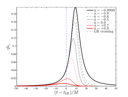
Figure 1: Time evolution of $-\dot{p}_{r_{*}}$: the characteristic time-scale of the curve $\tau_{\dot{p}_{r_{*}}}^{max}$ (Eq. (1)) is a measure of the adiabaticity of the plunge. One finds that $\tau_{\dot{p}_{r_{*}}}^{max}$ decreases from ${\hat{a}}=0.9$ to ${\hat{a}}=-0.57$ (see also Table 1), but then increases again. This is consistent with the increase of the quality factor $Q$ (indicating adiabaticity in the linear momentum flux) and the related peculiar time evolution of the recoil velocity as ${\hat{a}}\to-1$ (see Fig. 4). Note that $t_{\rm LR}$ indicates the light-ring crossing time.

The relative dynamics is started from post-circular initial data Buonanno and Damour (2000); Nagar et al. (2007) and driven from inspiral to plunge by the radiation reaction. The transition from quasi-circular inspiral to plunge depends on the spin-orbit coupling between the particle’s angular momentum and the black-hole’s spin through the Hamiltonian. It can be slowly-varying and adiabatic (spin aligned with particle’s angular momentum, the last-stable-orbit (LSO) moves towards the horizon) or quickly-varying and nonadiabatic (spin anti-aligned with particle’s angular momentum, the LSO moves away from the horizon). The net GW emission of linear momentum and the final value of the recoil velocity can be connected to the nonadiabatic part of the dynamics Damour and Gopakumar (2006). (A similar argument has also been discussed recently in Refs. Price et al. (2011, 2013)). In the following, we introduce a quantitative measure of this nonadiabaticity in the plunge phase.

Consider the time derivative of the radial momentum in a tortoise coordinate $-\dot{p}_{r_{*}}$ (changed sign for clarity; see Ref. Harms et al. (2014) for the precise definition). As shown in Ref. Harms et al. (2014) (see Fig. 15 there), $-p_{r_{*}}$ is a monotonic function of time: it grows during the plunge attaining a finite maximum at the horizon. Its time derivative has a bell shape as displayed in Fig. 1 for a few representative values of ${\hat{a}}$. For convenience of comparison, the plot is done versus $t-t_{\rm LR}$, where $t_{\rm LR}$ is the light-ring crossing time defined by $r_{\rm LR}\equiv r(t_{\rm LR})$ and $r_{\rm LR}=2\left[1+\cos\left(\frac{2}{3}\arccos(-{\hat{a}})\right)\right]$.

The spin-orbit interaction is repulsive for prograde orbits and attractive for retrograde orbits. Consistently, the distribution of $-\dot{p}_{r_{*}}$ is wider as ${\hat{a}}\to+1$ (slowly-varying, adiabatic plunge dynamics) and narrower as ${\hat{a}}\to-1$ (quickly-varying, nonadiabatic plunge dynamics). To quantify the spin-dependence of the width of the curve, we define its characteristic variation time

$$\tau_{\dot{p}_{r_{*}}}^{max}=-\dfrac{\dot{p}_{r_{*}}}{\dddot{p}_{r_{*}}}|_{t=t_{max}^{\dot{p}_{r_{*}}}}\ ,$$ (1)

where $t_{max}^{\dot{p}_{r_{*}}}$ corresponds to the peak of $-\dot{p}_{r_{*}}$. The values of $\tau_{\dot{p}_{r_{*}}}^{max}$ are listed in Table 1. Note that $\tau_{\dot{p}_{r_{*}}}^{max}$ is not monotonically decreasing when the spin decreases from positive to nearly-extremal negative values (it is not possible to deduce this from the plot). On the contrary, $\tau_{\dot{p}_{r_{*}}}^{max}$ attains a minimum for ${\hat{a}}\sim-0.57$ and grows again as ${\hat{a}}\to-1$ (though to smaller values), indicating that the dynamics becomes slightly more adiabatic again. Such a simple quantitative characterization of the plunge is helpful in interpreting the following analysis of the linear momentum flux and the recoil velocity.

III The GW linear momentum flux

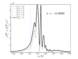
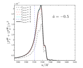
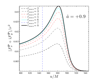
Figure 2: Modulus of the linear momentum flux for three representative values of ${\hat{a}}$. As ${\hat{a}}\to-1$, the emission of linear momentum occurs in a shorter time. The interference pattern seen for ${\hat{a}}=-0.9999$ is determined by the increased importance of the subdominant waveform multipoles with $0\leq m<\ell$ when ${\hat{a}}\to-1$ (as noted in Ref. Harms et al. (2014)) around merger (defined as the peak of $|\Psi_{22}|$, dashed vertical lines).

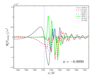
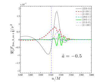
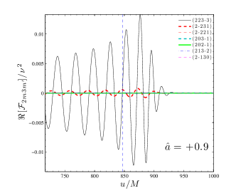
Figure 3: Comparing the real part of the various terms entering the leading contribution ${\cal F}_{2}^{\bf P}$ to the linear momentum flux, Eq. (III). One sees that for ${\hat{a}}=-0.9999$ all terms in Eqs. (4a)-(4g) have comparable magnitudes around merger (marked by the vertical line). This prompts the interference pattern seen in the corresponding modulus in Fig. 2.

Let us now analyze the GW linear momentum flux. We will see how the emission of linear momentum closely mirrors the plunge dynamics. Notably, the analysis of the flux (a gauge invariant quantity) is independent of having at hand a description of the dynamics and therefore can be directly applied to investigate also numerical relativity data.

In our simulations the GW linear momentum is emitted in the equatorial $xy$-plane because we consider equatorial orbits (the black hole spin is either aligned or antialigned with the orbital angular momentum). Working with RWZ-normalized variables $\Psi_{{\ell m}}^{(\epsilon)}$ the GW linear momentum flux reads

$${\cal F}_{x}^{\bf P}+{\rm i}{\cal F}_{y}^{\bf P}=\sum_{\ell=2}^{\ell_{max}}{\cal F}^{\bf P}_{\ell}=\dfrac{1}{8\pi}\sum_{\ell=2}^{\ell_{max}}\sum_{m=-\ell}^{\ell}{\rm i}\bigg{[}a_{{\ell m}}\dot{\Psi}_{\ell m}^{(0)}\dot{\Psi}^{(1)*}_{\ell,m+1}$$

$$+b_{\ell m}\sum_{\epsilon=0,1}\dot{\Psi}^{(\epsilon)}_{\ell m}\dot{\Psi}^{(\epsilon)*}_{\ell+1,m+1}\bigg{]},$$ (2)

where the numerical coefficients $(a_{\ell m},b_{\ell m})>0$ are given in Eqs. (16)-(17) of Bernuzzi and Nagar (2010), $\epsilon$ is the parity of $(\ell+m)$, and $\Psi^{*}_{{\ell m}}=(-1)^{m}\Psi_{\ell,-m}$. Note that for each value of $\ell$ the contribution ${\cal F}^{\bf P}_{\ell}$ involves all $\ell$ and $\ell+1$ waveform multipoles (e.g., for $\ell=2$ one deals with 7 waveform multipoles). Since we extracted gravitational wave multipoles up to $\ell_{max}=8$, we do not include $\ell=9$ modes in ${\cal F}^{\bf P}_{8}$.

Figure 2 shows the flux of linear momentum as a function of the retarded time $u$ (cf. Harms et al. (2014)) for ${\hat{a}}=-0.9999$ (top), ${\hat{a}}=-0.5$ (middle) and ${\hat{a}}=+0.9$ (bottom). Each labeled line on the plot corresponds to the sum $\sum_{\ell=2}^{\ell_{max}}{\cal F}^{\bf P}_{\ell}$ in Eq. (III) up to the indicated $\ell_{max}$. The vertical dashed line indicates the “merger time” $u_{\rm mrg}$, defined as the time of the peak of $|\Psi_{22}|$. To relate these figures with Fig. 1, as ${\hat{a}}\to-1$ one has $u_{\rm mrg}\approx t_{\rm LR}$, while as ${\hat{a}}\to 1$ one progressively gets $u_{\rm mrg}<t_{\rm LR}$. The precise quantitative information is collected in Table 4 of Harms et al. (2014): one has $t_{\rm LR}=7321.7$ for ${\hat{a}}=-0.9999$, $t_{\rm LR}=3321.3$ for ${\hat{a}}=-0.5$ and $t_{\rm LR}=883.6$ for ${\hat{a}}=+0.9$ [the corresponding last-stable-orbit (LSO) crossing times are 6858.3, 2980.4 and 820.7].

Comparing the three plots in Fig. 2 one can directly extract that as ${\hat{a}}\to-1$: (i) the emission of linear momentum appears more localized in time (the three time-axes show an equally-sized range of $\sim 140M$) , i.e. it becomes an impulsive phenomenon; (ii) the simple single-peak structure is replaced by a complicated interference pattern with several peaks of different amplitude and width.

This phenomenon mirrors strong destructive interference  effects between the various terms entering Eq. (III). Such effect is maximal as ${\hat{a}}\to-1$ and progressively less apparent as ${\hat{a}}$ increases. It can be explained (see below) by the magnification of the subdominant $0\leq m<\ell$ modes during the late plunge and merger as ${\hat{a}}\to-1$. Since it is present already in the leading-order ${\cal F}_{2}^{\bf P}$ term (dashed line in the bottom panel of Fig. 2) it can be quantitatively understood by analyzing the behavior of only this contribution as a function of the black hole spin.

Setting $\ell_{max}=2$ the corresponding GW linear momentum flux ${\cal F}_{2}^{\bf P}$ is built from the interference of the following seven terms, involving all $\ell=2$ and $\ell=3$ multipoles:

$${{\cal F}}_{2}^{\bf P} ={\cal F}_{223-3}+{\cal F}_{2-231}+{\cal F}_{2-221}$$

$$+{\cal F}_{202-1}+{\cal F}_{203-1}+{\cal F}_{213-2}+{\cal F}_{2-130}\ .$$ (3)

The ${\cal F}_{lm\ell^{\prime}m^{\prime}}$ are obtained from Eq. (III) and read explicitly

$${\cal F}_{223-3} =\dfrac{5}{\pi}\sqrt{\dfrac{6}{7}}\dot{\Psi}_{22}\dot{\Psi}_{3-3},$$ (4a)

$${\cal F}_{2-221} =\dfrac{2{\rm i}}{\pi}\dot{\Psi}_{2-2}\dot{\Psi}_{21},$$ (4b)

$${\cal F}_{2-231} =\dfrac{1}{\pi}\sqrt{\dfrac{10}{7}}\dot{\Psi}_{2-2}\dot{\Psi}_{31},$$ (4c)

$${\cal F}_{202-1} =\dfrac{{\rm i}}{\pi}\sqrt{6}\,\dot{\Psi}_{20}\dot{\Psi}_{2-1},$$ (4d)

$${\cal F}_{203-1} =\dfrac{2}{\pi}\sqrt{\dfrac{15}{7}}\dot{\Psi}_{20}\dot{\Psi}_{3-1},$$ (4e)

$${\cal F}_{213-2} =-\dfrac{1}{\pi}\dfrac{10}{\sqrt{7}}\,\dot{\Psi}_{21}\dot{\Psi}_{3-2},$$ (4f)

$${\cal F}_{2-130} =-\dfrac{1}{\pi}\sqrt{\dfrac{30}{7}}\dot{\Psi}_{2-1}\dot{\Psi}_{30}\ ,$$ (4g)

when using $\Psi^{*}_{{\ell m}}=(-1)^{m}\Psi_{\ell,-m}$.

References Harms et al. (2014); Taracchini et al. (2014) pointed out that the breakdown of the circularity during the plunge as ${\hat{a}}\to-1$ (see Fig. 15 in Ref. Harms et al. (2014)) makes each multipolar waveform amplitude higher and sharper around their peak (which occurs near merger). In particular for $0\leq m<\ell$ the peaks get amplified to values comparable to that of the leading $\ell=m=2$ mode (the effect is particularly striking for the $m=0$ modes). This phenomenon occurs on the short time scale of the plunge and thus also yields a magnification of the $\dot{\Psi}_{\ell m}$’s. One can then understand how the spin-dependence of the various ${\cal F}_{lm\ell^{\prime}m^{\prime}}$ terms in Eqs. (4) can prompt complicated interference patterns via Eq. (III). To illustrate how this works in practice, Fig. 3 compares the real part of the seven partial contributions given by Eq. (4) for spins ${\hat{a}}\in\{-0.9999,-0.5,+0.9\}$. For ${\hat{a}}=-0.9999$ all terms in Eq. (4) are comparable. One sees that ${\cal F}_{202-1}$ and ${\cal F}_{2-231}$ are approximately in phase among themselves and in phase opposition to ${\cal F}_{213-2}$ and ${\cal F}_{223-3}$. When taking the modulus of the sum of all these contributions one understands the origin of the minima in the modulus of Fig. 2. Notably, the times of the minima in Fig. 2 correspond to the minima of ${\cal F}_{202-1}$ and ${\cal F}_{2-231}$, indicating that the interference pattern of the linear momentum flux reflects the enhancement of $(\Psi_{20},\Psi_{21},\Psi_{31})$. This is driven by the next-to-quasi-circular corrections to the waveform, which are enhanced for the mainly radial indirect plunges.

By contrast, when ${\hat{a}}=+0.9$, ${\cal F}_{223-3}$ is much larger than the other terms, e.g. ${\cal F}_{2-231}$ and ${\cal F}_{202-1}$ do not contribute significantly. The negligible value of $\dot{\Psi}_{31}$ with respect to $\dot{\Psi}_{2-2}$ essentially removes the complicated behavior that one finds in ${\cal F}_{2-231}$ as ${\hat{a}}\to-1$, and this contribution is just dominated by the $\dot{\Psi}_{2-2}$ mode. Note in the bottom panel of Fig. 3 how the red and black lines are dephased by $\pi/2$, consistent with the dephasing due to complex conjugation.

Finally, focusing on the case ${\hat{a}}=-0.9999$ for definitess, we note that the emission of linear momentum predominantly occurs on the time interval $(7320,7360)$ around the largest peak of $|{\cal F}^{\bf P}|$; the interval is approximately the same where $-\dot{p}_{r_{*}}$ is significantly different from zero ($-\dot{p}_{r_{*}}$ peaks at $t^{p_{r_{*}}}_{max}\approx 7331$). This supports the understanding that it is the time variation of $p_{r_{*}}$ that is pumping up (the time-derivatives of) the gravitational waveform around the light-ring crossing to generate the narrow burst of linear momentum. For this value of the spin, we also note that the rather shallow peak of the flux around $u/M\sim 7390$ is essentially driven by the quasi-normal-mode excitation. For ${\hat{a}}=-0.9999$ the modes are long-lasting, which explains why this peak is so shallow (see also the top panel of Fig. 3). The same feature, with the same explanation, is seen also for ${\hat{a}}=-0.5$, though it is absent for ${\hat{a}}=+0.9$. We postpone to future work a detailed analysis of the QNMs-driven features of the linear momentum flux.

IV Kick and antikick

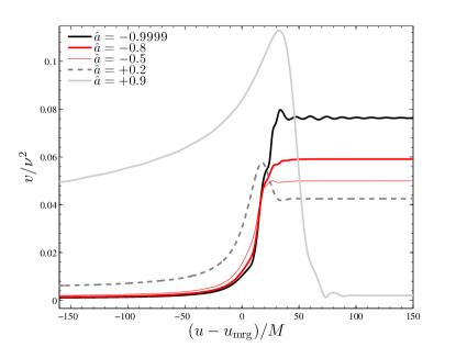
Figure 4: Time evolution of the recoil velocity for various black hole spin parameters ${\hat{a}}$. The large antikick present for positive values of ${\hat{a}}$ is progressively absorbed until it disappears when $-0.9\lesssim{\hat{a}}\lesssim-0.5$. Suprisingly, for nearly-extremal negative spins it progressively reappears due to a slight increase of the adiabatic character of the plunge dynamics. We use the peak of $|\Psi_{22}|$ as the merger time $u_{\rm mrg}$.

Table 1: From left to right the columns report: the magnitude of the final and the maximal recoil velocities, $v_{end}/\nu^{2}$ and $v_{max}/\nu^{2}$; the magnitude of the antikick $\Delta v/\nu^{2}$: for $-0.9\leq{\hat{a}}\leq-0.5$ no significant antikick is observed; the quality factor $Q$ associated with the maximum of the amplitude of the linear momentum flux, as an indicator of the adiabaticity of the emission of linear momentum. The larger is $Q$ the more adiabatic is the emission process, the larger is the antikick; the characteristic time scale $\tau_{\dot{p}_{r_{*}}}^{max}$ of $-\dot{p}_{r_{*}}$ (see Eq. (1)), as a complementary indicator of the adiabaticity of the dynamics; the approximate analytic calculation of the kick velocity, $v_{end}^{anal}/\nu^{2}$ of Eq. (9). Minima of $\Delta v/\nu^{2},Q,\tau_{\dot{p}_{r_{*}}}^{max}$ are printed in boldface.

${\hat{a}}$	$v_{max}/\nu^{2}$	$v_{end}/\nu^{2}$	$\Delta v/\nu^{2}$	$Q$	$\tau^{max}_{\dot{p}_{r_{*}}}$	$v_{end}^{anal}/\nu^{2}$
-0.9999	0.07972	0.07634	3.377e-03	1.0060	3.8436	0.04060
-0.9990	0.07967	0.07637	3.303e-03	1.0065	3.8411	0.04091
-0.9950	0.07884	0.07587	2.972e-03	0.9942	3.8302	0.04052
-0.9900	0.07798	0.07539	2.589e-03	0.9639	3.8171	0.04050
-0.9800	0.07571	0.07383	1.883e-03	0.9518	3.7924	0.04017
-0.9700	0.07452	0.07320	1.326e-03	0.9356	3.7696	0.03996
-0.9500	0.07093	0.07040	5.264e-04	0.9015	3.7292	0.03942
-0.9000	0.06545	0.06539	5.589e-05	0.8663	3.6508	0.03855
-0.8000	0.05910	0.05909	9.332e-06	0.8378	3.5570	0.03807
-0.7000	0.05501	0.05501	8.223e-07	0.8402	3.5123	0.03910
-0.6000	0.05183	0.05183	1.915e-08	0.8650	3.4977	0.04189
-0.5000	0.05003	0.05003	2.289e-09	0.9024	3.5044	0.04765
-0.4400	0.04914	0.04879	3.485e-04	0.9491	3.5167	0.05318
-0.4000	0.04948	0.04882	6.618e-04	1.0038	3.5280	0.05801
-0.3000	0.04913	0.04766	1.479e-03	1.9191	3.5667	0.09562
-0.2000	0.04981	0.04658	3.224e-03	1.4625	3.6198	0.09148
-0.1000	0.05060	0.04534	5.266e-03	1.4011	3.6878	0.07821
0.0000	0.05319	0.04530	7.892e-03	1.4364	3.7722	0.07029
0.1000	0.05471	0.04377	1.094e-02	1.5086	3.8755	0.06279
0.2000	0.05771	0.04252	1.519e-02	1.6045	4.0019	0.05655
0.3000	0.06105	0.04053	2.052e-02	1.7207	4.1580	0.05116
0.4000	0.06606	0.03822	2.785e-02	1.8678	4.3534	0.04578
0.5000	0.07131	0.03398	3.733e-02	2.0643	4.6049	0.03887
0.6000	0.07796	0.02831	4.965e-02	2.3413	4.9426	0.02766
0.7000	0.08719	0.02056	6.663e-02	2.7528	5.4289	0.01406
0.8000	0.09919	0.01085	8.835e-02	3.5249	6.2242	0.00431
0.9000	0.11293	0.00206	1.109e-01	5.3834	7.8682	0.00031

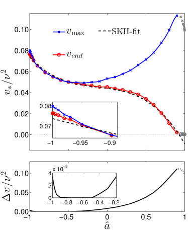
Figure 5: Dependence of the maximum (blue, crosses) and the final (red, circles) recoil velocities on the spin ${\hat{a}}$ for $\nu=10^{-3}$. The dashed black line refers to the fit of  Sundararajan et al. (2010). Although the antikick is suppressed in the interval $-0.9\leq{\hat{a}}\leq-0.5$, it strikes back for large negative spins , i.e. for ${\hat{a}}\lesssim-0.9$ we find again that $v_{max}>v_{end}$. The data points for ${\hat{a}}>0.9$ are plotted in gray to indicate that they are affected by larger systematic uncertainties due to inaccuracy of the radiation reaction as ${\hat{a}}\rightarrow+1$ ($v_{max}$ is expected to grow monotonically. See Appendix A).

Let us now discuss the recoil velocity computation and the antikick. We define a complex velocity vector $\mathbf{v}\equiv v_{x}+{\rm i}v_{y}$ corresponding to the recoil velocity accumulated by the system up to a certain time $t$,

$$\mathbf{v}=-\dfrac{1}{M}\int_{-\infty}^{t}dt^{\prime}\ \left({\cal F}_{x}^{\bf P}+{\rm i}{\cal F}_{y}^{\bf P}\right)\ .$$ (5)

In practice, the improper integral above is calculated from a finite initial time $t_{0}$. Thus the recoil velocity calculation requires to fix a complex integration constant $\mathbf{v}_{0}$ that accounts for the velocity that the system has acquired in evolving from $t=-\infty$ to $t=t_{0}$, i.e

$$\mathbf{v}=\mathbf{v}_{0}-\dfrac{1}{M}\int_{t_{0}}^{t}dt^{\prime}\left({\cal F}_{x}^{\bf P}+{\rm i}{\cal F}_{y}^{\bf P}\right).$$ (6)

If this integration constant is not determined correctly, unphysical oscillations show up in the time evolution of the modulus of the velocity $v(t)\equiv|\mathbf{v}(t)|$, which eventually result in an inaccurate estimate of the final recoil. We determine the vectorial integration constant $\mathbf{v}_{0}$ by finding the center of the hodograph of the velocity in the complex plane following Pollney et al. (2007); Bernuzzi and Nagar (2010). This procedure is tuned iteratively until the time evolution of $v(t)$ during inspiral grows monotonically without spurious oscillations. The correct determination of the integration constant is especially important when ${\hat{a}}\to+1$, as it can strongly influence the rather small value of the final recoil velocity.

Figure 4 shows for some representative configurations ${\hat{a}}\in\{-0.9999,-0.8,-0.5,+0.2,+0.9\}$ the computed time evolution of the recoil velocity. Visually the ascent of the curves is free of oscillations due to the fine tuned setting of $\mathbf{v}_{0}$. Close to merger $v(t)$ grows monotonically until it reaches its maximum $v_{max}$. For large positive spins it then drops down to an asymptotic value $v_{end}<v_{max}$. The gap $\Delta v=v_{max}-v_{end}$ between the maximal and the final recoil velocity is called the antikick. We list in Table 1 the values of the maximal and final recoil velocities as well as the antikick for the configurations considered in this work. The antikick is large for positive spins and essentially absent for $-0.9\leq{\hat{a}}\leq-0.5$. Our data highlight a new feature of the antikick for nearly-extremal, negative spins: the antikick “strikes back” for $-1<{\hat{a}}<-0.9$, i.e. $\Delta v$ increases again, though it reaches smaller values than for positive spins. From the value $\Delta v/\nu^{2}\sim 6\times 10^{{-5}}$ at ${\hat{a}}=-0.9$, it rises to $1.3\times 10^{-3}$ at ${\hat{a}}=-0.97$ and reaches $\sim 3.4\times 10^{-3}$ in the most extremal case considered (${\hat{a}}=-0.9999$). This value is comparable to values obtained for ${\hat{a}}\sim-0.2$. The behavior of the recoil velocities and the antikick versus ${\hat{a}}$ is illustrated in Figure 5. The top panel shows the maximal and final recoil velocities. The SKH fit is included for comparison. The bottom panel shows the antikick. Note that in the range $-0.9\leq{\hat{a}}\leq+0.9$ our data are compatible (though different because of different accuracy, see Appendix A) with SKH findings.

The reappearance of the antikick, although apriori surprising, can be understood quantitatively in relatively simple terms following DG. One of the points of DG was to relate the antikick to the maximum of the modulus of the GW linear momentum flux, ${\cal F}_{\bf P}^{max}=\max|{\cal F}_{\bf P}|$. At time $t$, the accumulated kick velocity is given by the complex integral (5), i.e. $\mathbf{v}={\rm i}\int_{-\infty}^{t}|{\cal F}_{\bf P}(t)|e^{i\varphi(t)}dt$, where $\varphi(t)$ is the phase of the linear momentum flux. Expanding around the time $t_{max}$ corresponding to ${\cal F}_{\bf P}^{max}$ one gets

$$\mathbf{v}\simeq{\rm i}{\cal F}_{\bf P}^{max}e^{{\rm i}\varphi_{max}}\sqrt{\dfrac{\pi}{2\alpha}}e^{\beta^{2}/(2\alpha)}{\rm erfc}(z),$$ (7)

with $z=-\sqrt{\alpha/2}(\bar{t}-\beta/\alpha)$, where $\alpha\equiv 1/\tau_{max}^{2}(1-{\rm i}\epsilon_{max})$ and $\beta={\rm i}Q/\tau_{max}$. Here $\tau^{2}_{max}\equiv-{\cal F}_{\bf P}^{max}/(\ddot{|{\cal F}|}_{\bf P})^{max}$ is the characteristic time scale associated with the “resonance peak” of $|{\cal F}_{\bf P}|$; $\omega\equiv\dot{\varphi}$, $\epsilon_{max}\equiv\dot{\omega}_{max}\tau^{2}_{max}$, and the quantity

$$Q\equiv\omega_{max}\tau_{max},$$ (8)

can be interpreted as the quality factor associated with the same peak. According to Eq. (7) the time evolution of the recoil velocity is given by the complementary error function ${\rm erfc}(z)$ of a complex argument $z$ whose imaginary part is proportional to the quality factor $Q$. Hence, the quality factor $Q$ controls the monotonic behavior of ${\rm erfc}(z)$: when $Q$ is sufficiently large a local maximum appears.

The values of $Q$ are listed in Table 1 for all configurations considered. One observes immediately the tight correlations between $Q$, $v_{end}$, $\Delta v$ and $\tau_{\dot{p}_{r_{*}}}^{max}$, which supports the interpretation of the antikick results. The quantities $\tau_{\dot{p}_{r_{*}}}^{max}$ and $Q$ behave qualitatively like $\Delta v$, i.e. their minima at ${\hat{a}}\sim(-0.5,-0.58,-0.75$) for ($\Delta v$, $\tau_{\dot{p}_{r_{*}}}^{max}$, $Q$) are close and all of them increase again when ${\hat{a}}\to-1$. Physically the quality factor can be interpreted as a measure of the adiabaticity of the process: small $Q$ indicates fast emission of linear momentum and reduced antikick; large $Q$ indicates slow emission of linear momentum and enhanced antikick. Thus, the computation of $Q$ from the maximum of the linear momentum flux gives us a quantitative method to understand the origin of the antikick and, in particular, to predict its behavior for ${\hat{a}}\to-1$ (see Fig. 5). Although $Q$ is quantitative and helpful in understanding the global picture, it might be missing some details. For example, Table 1 says that $Q$ is in one to one correspondence with $\Delta v$ and $\tau^{\rm max}_{p_{r_{*}}}$ for all values of ${\hat{a}}$ except in the range $-0.4<{\hat{a}}<0$, where it seems to oscillate instead of growing monotonically as the values of $\Delta v$ suggest. Actually, inspecting $|{\cal F}_{\bf P}|$ for, say, ${\hat{a}}=-0.3$ (that shows the largest deviation from the global growing trend) one finds that it has a rather shallow top region, with essentially two maxima of approximately the same height fused together. In this particular case, the approximation that is behind the computation of $Q$ is probably not accurate enough to faithfully represent the structure of the peak of $|{\cal F}_{\bf P}|$ .

Finally, following DG, when $t\gg\tau_{max}$, the error function in Eq. (7) can be evaluated analytically to give the final recoil magnitude

$$v^{anal}_{end}\simeq\sqrt{2\pi}{\cal F}_{\bf P}^{max}\dfrac{\tau_{max}}{(1+\epsilon^{2}_{max})^{1/4}}e^{-Q^{2}/[2(1+\epsilon^{2}_{max})]}\quad.$$ (9)

Looking at Table 1 the computed $v^{anal}_{end}$ is at the same order as $v_{end}$ over the whole spin range. Percentual differences usually vary around $\sim 50\%$ but can reach $\sim 10\%$ for values around ${\hat{a}}\sim 0.6$. It would be interesting to increase the order of the approximation of formula (7) and recheck its domain of accuracy depending on ${\hat{a}}$. Such formula would simplify the computation of the final recoil from numerical relativity data, especially because one would rely only on local knowledge of the linear momentum flux avoiding the uncertainties related to the integration constant.

V Conclusions

The main finding of this paper is a new phenomenon for nearly extremal negative spins. The antikick, i.e. the drop from the maximal to the final recoil velocity, is not a monotonic function of the spin and, while suppressed between $-0.9\leq{\hat{a}}\leq-0.5$, it reappears for nearly extremal negative spins. Quantitatively, this surprising phenomenon is a small but significant effect, and its existence allows us to get a new understanding of the dynamics of retrograde plunges. It can be interpreted quantitatively and predicted qualitatively by analyzing the plunge dynamics or the GW linear momentum flux around its maximum. The variation of the latter can be measured by the quality factor $Q$, which can also be viewed as a measure of the “adiabaticity” of the process of emission of linear momentum through GWs. A significant antikick always results from a slow (quasi-adiabatic) plunge and is associated with large values of $Q$. Small values of $Q$ mirror a rather nonadiabatic plunge and, consistently, small, or absent, antikicks.

In this work we have pointed out how certain features of the linear momentum flux directly mirror the dynamics. Qualitatively, our findings may be robust also in unequal but comparable mass-ratio binaries, in which the ratio between the spin of the two objects is nearly extremal. The flux analysis presented here may guide the extraction of useful information for kick computations in numerical relativity, like those recently performed in Healy et al. (2014).

Appendix A Accuracy

Table 2: Dependence on $\ell_{max}$ of $v_{end}$ and $v_{max}$. For ${\hat{a}}=-0.9999$, $\ell_{max}>4$ contributions give less than $1\%$. For ${\hat{a}}=+0.9$, the effect is larger and $v_{end}$ slightly increases for higher $\ell_{max}$.

${\hat{a}}=-0.9999$
$\ell_{max}$	$v_{max}/\nu^{2}$	diff $[\%]$	$v_{end}/\nu^{2}$	diff $[\%]$
2	0.070252	-	0.068323	-
3	0.077692	10.59	0.074520	9.07
4	0.079033	1.73	0.075589	1.43
5	0.079187	0.19	0.075766	0.23
6	0.079442	0.32	0.076045	0.37
7	0.079613	0.21	0.076228	0.24
8	0.079722	0.14	0.076345	0.15

${\hat{a}}=+0.9$
$\ell_{max}$	$v_{max}/\nu^{2}$	diff $[\%]$	$v_{end}/\nu^{2}$	diff $[\%]$
2	0.003687	-	0.000932	-
3	0.045957	1146.49	0.001190	27.80
4	0.074009	61.04	0.001350	13.43
5	0.091701	23.90	0.001535	13.64
6	0.102239	11.49	0.001741	13.44
7	0.108800	6.42	0.001917	10.10
8	0.112927	3.79	0.002056	7.27

Table 3: Effect of the mass ratio $\nu$. The table compares for a few values of ${\hat{a}}$ the recoil velocities as obtained from trajectories with $\nu=10^{-3}$ and $\nu=10^{-4}$. The percentual difference if about $1\%$ for ${\hat{a}}<0.9$ and reaches $\sim 7\%$ for ${\hat{a}}=0.9$. We use the notation $v^{(\log_{10}\nu)}$.

${\hat{a}}$	$v_{max}^{(-3)}/\nu^{2}$	$v_{max}^{(-4)}/\nu^{2}$	diff $[\%]$	$v_{end}^{(-3)}/\nu^{2}$	$v_{end}^{(-4)}/\nu^{2}$	diff $[\%]$
-0.9000	0.06545	0.06598	0.81	0.06539	0.06592	0.81
-0.7000	0.05501	0.05504	0.06	0.05501	0.05504	0.06
-0.5000	0.05003	0.04964	0.76	0.05003	0.04964	0.76
0.0000	0.05319	0.05313	0.11	0.04530	0.04508	0.48
0.5000	0.07131	0.07119	0.17	0.03398	0.03383	0.44
0.7000	0.08719	0.08877	1.81	0.02056	0.02073	0.83
0.9000	0.11293	0.12093	7.09	0.00206	0.00199	3.24

We give here some estimates about the accuracy of our computation and discuss the limitations of our approach for configurations with ${\hat{a}}\to+1$.

Table 2 shows the effect of $\ell_{max}$ on the velocity computation. The results for ${\hat{a}}=-0.9999$ vary $\lesssim 1\%$ by including multipoles with $\ell_{max}>4$. The inclusion of high multipoles is more relevant for large positive spins. For ${\hat{a}}=+0.9$ we observe a $\sim 7\%$ variation by increasing $\ell_{max}=7$ to $\ell_{max}=8$. Including only up to $\ell_{max}=6$ multipoles underestimates $v_{end}$ by at least $10\%$. This is consistent with the corresponding variations we see in the fluxes, Fig. 2. Note that $v_{end}$ increases by including more multipoles.

Another source of uncertainty is the finite value of the mass ratio $\nu$ employed in the simulations Bernuzzi and Nagar (2010). Table 3 shows a comparison between results obtained with $\nu=10^{-3}$ and $\nu=10^{-4}$. The uncertainties for ${\hat{a}}<0.5$ are at the $1\%$ level. For larger spins they grow and reach about $7\%$ for ${\hat{a}}=0.9$. We expect even larger uncertainties for ${\hat{a}}\geq 0.95$ since these simulations are strongly biased by the inaccurate radiation reaction (see below).

Our kick calculation in Table 1 and Fig. 5 can be compared with the fit proposed in SKH. The latter was calculated (i) including multipoles up to $m_{max}=6$; (ii) using a different technique to determine the integration constant; and (iii) using $\nu=10^{-4}$ simulations of about $25$ orbits. The fit of SKH refers to the interval $|{\hat{a}}|<0.9$ and is therein consistent with our data, in some cases within $1\%$. However, it does not capture the fine structures for nearly-extremal values of the spin. Observe, for example, that it underestimates $v_{end}$ for ${\hat{a}}\to-1$ (Fig. 5).

Let us finally discuss the data for nearly-extremal positive spins $+0.9<{\hat{a}}\leq+0.9999$. These data are displayed in Fig. 5 in gray color since they are uncertain. The numbers behind the plot are listed in Table 4. Inspecting the table and Fig. 5 one sees that: (i) $v_{end}$ first decreases and then remains approximately constant (and very small) for ${\hat{a}}\geq 0.995$; (ii) $v_{max}$ decreases monotonically; (iii) $Q$ oscillates around 9.2 for $0.99\leq{\hat{a}}\leq 0.9999$; (iv) $\tau^{max}_{\dot{p}_{r_{*}}}$ increases monotonically. At first sight these numbers look contradictory. The increase of $\tau^{max}_{\dot{p}_{r_{*}}}$ with ${\hat{a}}$ is indicating that the dynamics (and thus the emission of linear momentum) is increasingly adiabatic as ${\hat{a}}\to+1$. Consistently, $v_{end}$ decreases, but the increased adiabaticity of the dynamics is not mirrored in $Q$ nor in $v_{max}$, which decreases instead.

Table 4: Same as Table 1 for$+0.95\leq{\hat{a}}\leq+0.9999$.

${\hat{a}}$	$v_{max}/\nu^{2}$	$v_{end}/\nu^{2}$	$\Delta v/\nu^{2}$	$Q$	$\tau^{max}_{\dot{p}_{r_{*}}}$	$v_{end}^{anal}$
0.9500	0.11186	0.00065	1.112e-01	7.1404	8.6964	0.00015
0.9700	0.10821	0.00046	1.077e-01	7.9190	8.8428	0.00008
0.9800	0.10524	0.00043	1.048e-01	8.7525	9.0199	0.00021
0.9900	0.10307	0.00044	1.026e-01	9.2251	9.4295	0.00045
0.9950	0.10127	0.00038	1.009e-01	9.3933	9.8429	0.00039
0.9990	0.09968	0.00036	9.933e-02	9.2492	10.4124	0.00019
0.9999	0.09914	0.00035	9.878e-02	9.1388	10.5938	0.00031

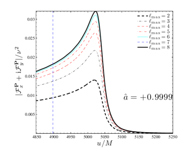
Figure 6: Flux of linear momentum for ${\hat{a}}=+0.9999$. The vertical line indicates the peak of $|\Psi_{22}|$.

A careful inspection of the dynamics brought us to conclude that these results are qualitatively inaccurate for $v_{max}$ (and thus $Q$) and quantitatively inaccurate for $v_{end}$. The main reason is the systematic inaccuracy of the radiation reaction for large positive spins ${\hat{a}}\gtrsim 0.9$, as shown in Harms et al. (2014). Practically speaking, the low accuracy of the radiation reaction (and in particular the absence of horizon fluxes that could contrast the loss of angular momentum to infinity via superradiance Bernuzzi et al. (2012); Taracchini et al. (2013)) makes the system lose too much angular momentum. For ${\hat{a}}>+0.97$ this effect is so strong that the angular momentum $p_{\phi}$ becomes negative ($p_{\phi}\sim-0.1$) around merger. For example, for $a+0.9999$ (see Fig. 6) this change of sign occurs at $t/M=5038$, that is quite close to the peak of the flux of linear momentum in a domain where the waveforms are still influenced by the dynamics (the LSO is crossed at $t/M=5056.6$ and the light-ring at $t/M=5220$). This unphysical effect ($p_{\phi}$ is defined to be positive) mirrors an excessive acceleration of the dynamics during the plunge and heuristically explains the drop of $v_{max}$ for ${\hat{a}}>0.9$. By contrast, we found that the calculation of $\tau^{max}_{\dot{p}_{r_{*}}}$ relies on a part of the dynamics before the change of sign of $p_{\phi}$ ($-\dot{p}_{r_{*}}$ peaks at $t/M=5028$) and therefore is more robust, as confirmed by the monotonic behavior of $\tau^{max}_{\dot{p}_{r_{*}}}$ over ${\hat{a}}$. A way of treating larger spin values is to adopt the self-consistent radiation reaction method introduced in Harms et al. (2014). Doing this is computationally very demanding and will be discussed in a follow up study. At present, we could check our understanding only against self-consistent ${\hat{a}}=+0.9$ data Harms et al. (2014). Consistently with our expectation that the correct radiation reaction should yield a more adiabatic plunge, we found a slightly smaller $v_{end}^{\rm sc}/\nu^{2}=0.00189$ (instead of 0.00206) and a slightly larger $v_{max}^{\rm sc}/\nu^{2}=0.11908$ (instead of 0.11293). This preliminary result suggests that $v_{max}$ will increase further and $v_{end}$ will become smaller as ${\hat{a}}\to+1$. New, challenging investigations will be needed to assess whether $v_{end}=0$ as ${\hat{a}}=+1$.

References

- Nagar (2013) A. Nagar, Phys.Rev. D88, 121501 (2013), eprint 1306.6299.
- Bernuzzi and Nagar (2010) S. Bernuzzi and A. Nagar, Phys. Rev. D81, 084056 (2010), eprint 1003.0597.
- Sundararajan et al. (2010) P. A. Sundararajan, G. Khanna, and S. A. Hughes, Phys.Rev. D81, 104009 (2010), eprint 1003.0485.
- Baker et al. (2006) J. G. Baker, J. Centrella, D.-I. Choi, M. Koppitz, J. R. van Meter, et al., Astrophys.J. 653, L93 (2006), eprint astro-ph/0603204.
- Schnittman et al. (2008) J. D. Schnittman et al., Phys. Rev. D77, 044031 (2008), eprint 0707.0301.
- Harms et al. (2014) E. Harms, S. Bernuzzi, A. Nagar, and A. Zenginoglu (2014), eprint 1406.5983.
- Damour and Gopakumar (2006) T. Damour and A. Gopakumar, Phys. Rev. D73, 124006 (2006), eprint gr-qc/0602117.
- Price et al. (2011) R. H. Price, G. Khanna, and S. A. Hughes, Phys.Rev. D83, 124002 (2011), eprint 1104.0387.
- Price et al. (2013) R. H. Price, G. Khanna, and S. A. Hughes, Phys.Rev. D88, 104004 (2013), eprint 1306.1159.
- Rezzolla et al. (2010) L. Rezzolla, R. P. Macedo, and J. L. Jaramillo, Phys.Rev.Lett. 104, 221101 (2010), eprint 1003.0873.
- Damour and Nagar (2014) T. Damour and A. Nagar (2014), eprint 1406.6913.
- Nagar et al. (2007) A. Nagar, T. Damour, and A. Tartaglia, Class. Quant. Grav. 24, S109 (2007), eprint gr-qc/0612096.
- Damour et al. (2009) T. Damour, B. R. Iyer, and A. Nagar, Phys. Rev. D79, 064004 (2009), eprint 0811.2069.
- Pan et al. (2011) Y. Pan, A. Buonanno, R. Fujita, E. Racine, and H. Tagoshi, Phys.Rev. D83, 064003 (2011), eprint 1006.0431.
- Nagar and Akcay (2012) A. Nagar and S. Akcay, Phys.Rev. D85, 044025 (2012), eprint 1112.2840.
- Taracchini et al. (2013) A. Taracchini, A. Buonanno, S. A. Hughes, and G. Khanna, Phys.Rev. D88, 044001 (2013), eprint 1305.2184.
- Taracchini et al. (2014) A. Taracchini, A. Buonanno, G. Khanna, and S. A. Hughes (2014), eprint 1404.1819.
- Harms et al. (2013) E. Harms, S. Bernuzzi, and B. Brügmann, Class.Quant.Grav. 30, 115013 (2013), eprint 1301.1591.
- Shah (2014) A. G. Shah (2014), eprint 1403.2697.
- Buonanno and Damour (2000) A. Buonanno and T. Damour, Phys. Rev. D62, 064015 (2000), eprint gr-qc/0001013.
- Bini and Damour (2012) D. Bini and T. Damour, Phys.Rev. D86, 124012 (2012), eprint 1210.2834.
- Pollney et al. (2007) D. Pollney, C. Reisswig, L. Rezzolla, B. Szilagyi, M. Ansorg, et al., Phys.Rev. D76, 124002 (2007), eprint 0707.2559.
- Healy et al. (2014) J. Healy, C. O. Lousto, and Y. Zlochower (2014), eprint 1406.7295.
- Bernuzzi et al. (2012) S. Bernuzzi, A. Nagar, and A. Zenginoglu, Phys.Rev. D86, 104038 (2012), eprint 1207.0769.