On a consistent finite-strain plate theory based on 3-D energy principle

Abstract

This paper derives a finite-strain plate theory consistent with the principle of stationary three-dimensional (3-D) potential energy under general loadings with a third-order error. Staring from the 3-D nonlinear elasticity (with both geometrical and material nonlinearity) and by a series expansion, we deduce a vector plate equation with three unknowns, which exhibits the local force-balance structure. The success relies on using the 3-D field equations and bottom traction condition to derive exact recursion relations for the coefficients. Associated weak formulations are considered, leading to a 2-D virtual work principle. An alternative approach based on a 2-D truncated energy is also provided, which is less consistent than the first plate theory but has the advantage of the existence of a 2-D energy function. As an example, we consider the pure bending problem of a hyperelastic block. The comparison between the analytical plate solution and available exact one shows that the plate theory gives second-order correct results. Comparing with existing plate theories, it appears that the present one has a number of advantages, including the consistency, order of correctness, generality of the loadings, applicability to finite-strain problems and no involvement of unphysical quantities.

1 Introduction

Plates are very important engineering structures, which have attracted extensive research since the 19th century. Plates are defined as plane structural elements with a small thickness (characteristic length $h$) compared with the other two planar dimensions. Plate theories attempt to reduce the three-dimensional (3-D) elasticity theory to a 2-D approximate one defined on a surface. The literature on plate theories is vast, including direct [2, 1] and derived plate theories. Here, we only give a review on selected works on derived plate theories, which are

divided into three categories.

(1) A common starting point is the series expansion of the deformed position (or displacement) vector in terms of thickness variable $Z$, like

$$\mathbf{x}(\mathbf{r},Z)=\sum_{j=0}^{N}Z^{j}\mathbf{x}^{(j)}(\mathbf{r}).$$ (1)

Early attempts on plate theories relied on a priori hypotheses, mostly motivated by engineering intuition. The classical plate theory (Kirchhoff-Love theory, see Kirchhoff [3] and Love [4]), which relies on three assumptions about both the geometry and deformation, is known to be only applicable to thin plates. Within linear elasticity, the first-order shear deformable plate theory [5] (Mindlin-Reissner theory) relaxes one of Kirchhoff’s assumptions, and introduces additional two unknowns. As a refinement, the third-order shear deformable plate theory [6, 7] incorporates postulated cubic terms in the two planar displacements, by assuming the way that the stresses vary over a cross-section. The advantage is that it avoids the use of the shear correction factor, whereas the results for $\mathbf{x}$ are almost the same as in Mindlin-Reissner theory (see [7]). The von Kármán plate theory [8] still uses Kirchhoff’s assumptions but retains some nonlinear components for the strain tensor (geometric nonlinearity) with an attempt to describe large deflections for thin plates. Although widely accepted and used, due to the hypotheses involved, one cannot expect that they are consistent with the 3-D formulation up to the required order for general loadings. Also, they do not expect to provide good results for relatively thick plates and certainly cannot be used for finite-strain problems.

(2) Another approach is also based on $(\ref{eq0})$ but with no explicit kinematic assumptions. All the coefficients $\mathbf{x}^{(j)}$ ($j\geq 1$) are treated as independent unknowns, whose governing equations are derived from the 2-D variational (or virtual work) principle by first integrating out the $Z$ variable and conducting a truncation. Such an approach was adopted by Kienzler [9, 10] based on linear elasticity. By a procedure of "pseudo-reduction" of the resulting system to certain orders of $h$, the classical plate theory and a Reissner-type theory [11, 12] were recovered. Based on nonlinear elasticity, Meroueh [13] used a similar approach except with Legendre polynomials of $Z$ in $(\ref{eq0})$, and formulated a system in terms of generalized (higher-order) stress resultants for finite-strain problems. Also based on nonlinear elasticity, Steigmann [14] carried out a study to construct an $O(h^{3})$ 2-D energy and finally arrived at a fourth-order system for $\mathbf{x}^{(0)}$ by eliminating other unknowns $\mathbf{x}^{(j)}$ ($j\geq 1$). The disadvantage of these theories is that the resulting system (Euler-Lagrange equation) contains many unknowns, albeit some may be eliminated by a further reduction. In addition, it is not easy to interpret and propose suitable and consistent boundary conditions on the lateral surface, since they involve generalized (high-order) stress resultants whose physical meanings are not clear. Also, as pointed out by Steigmann [15], for the truncated energy to be as accurate as possible by the standard of 3-D elasticity theory, one needs to impose restrictions on the high-order coefficients in $(\ref{eq0})$ from the 3-D formulation instead of treating them as independent unknowns. This way was adopted by Steigmann in [16, 17, 15], leading to a significant progress towards the derivation of more proper plate and shell models which incorporate both stretching and bending. More specifically, the author considered the case that the tractions were zero (or sufficiently small) on the top and bottom surfaces, which were utilized to represent $\mathbf{x}^{(i)}$ ($i=1,2$) in terms of $\mathbf{x}^{(0)}$, leading to a final system with only $\mathbf{x}^{(0)}$. The theory appears to extend Koiter’s shell theory [18] and dictate an optimal $O(h^{3})$ approximation for the 3-D potential energy. However, as indicated by the author in [15], an undesirable feature is that the relation for $\mathbf{x}^{(1)}$ is not accurate enough, which may cause a non-negligible $O(h^{3})$ error in the energy. And, the theory is restricted to the traction-free (or sufficiently small traction) case.

(3) Some consistent mathematical approaches for deriving leading-order plate theories have also been developed, which are based on certain a priori scalings between the thickness $h$ and the deformations (or applied loads). The method of Gamma convergence [19, 20, 21] concerns with the limiting 2-D variational problem of vanishing thickness $h$, which leads to a hierarchy of 2-D energies depending on the scalings. This method is rigorous but so far has failed to furnish a model containing the thickness parameter which incorporates both bending and stretching. On the other hand, asymptotic methods [22, 23, 24] aim at generating the leading-order (in $h$) 2-D variational problem or differential system via formal expansions. In [22], it was shown that von Kármán plate equations could be derived formally by such an approach based on the 3-D weak formulation with prescribed orders of applied loads and certain lateral surface boundary conditions. In [23, 24], the derivations were based on the 3-D differential formulation, in particular a hierarchy of leading-order plate equations were derived in [24]. However, the main difficulty preventing the wide applicability of these models is that they do not furnish a single plate model for all orders of applied loads, which is perhaps most needed in engineering problems. There are also some restrictions on the lateral boundary conditions in the asymptotic approaches. And, from the leading-order equations, it is difficult to examine the effects of the thickness.

Strictly speaking, a plate theory can be said to be consistent if the approximations ensure that either the 3-D differential formulation (including field equations and boundary conditions) or the 3-D weak formulation (by the energy principle) are satisfied to the required order of $h$. In our view, a good plate theory should be consistent with the 3-D formulation beyond the leading order with no special restrictions on applied loads, and further should furnish a single model with no unphysical quantities, leading to applicability from thin plates to relatively thick plates for a variety of deformations from small bending and stretching to finite strains. Despite more than 150 years research and significant advancements (see the above review for selected works), it appears that such a good plate theory has not been established. In this paper, an attempt is made in this direction.

Our starting point is also $(\ref{eq0})$ (with $N=4$). With this expansion and based on 3-D nonlinear elasticity, we intend to derive (without special restrictions on applied loads) a 2-D plate system consistent with the 3-D stationary potential energy principle (or weak formulation) with an error of $O(h^{4})$, with an aim of producing $O(h^{2})$-correct results for all the displacement (position) vector, strain tensor and stress tensor. We mention some key points for our success. First, rather than obtaining a truncated 2-D energy by integration, we deduce the main results by directly approximating the exact 3-D field equations and conditions on the top and bottom surfaces. This was the way adopted before (with only third-order material nonlinearity) in [25, 26, 27] for deriving rod-like theories and in [28] for deriving a plate model involving only stretching. Specifically, those 3-D differential relations are kept to the desired order in a pointwise manner, such that the corresponding terms in the variation of the 3-D potential energy are $O(h^{4})$. A finding is that the exact recursive relations between $\mathbf{x}^{(i)}(i=2,3,4)$ and $\mathbf{x}^{(i)}(i=0,1)$ can be obtained by solving linear algebraic equations. Second, we adopt an expansion about the bottom surface, as did in [29] for a tube buckling problem. This enables us to derive an exact algebraic relation between $\mathbf{x}^{(1)}$ and $\nabla\mathbf{x}^{(0)}$, which avoids the non-negligible error in [15]. These relations show the dependence among $\mathbf{x}^{(i)}(i=0,1,2,3,4)$, and thus it may not be proper to treat them as independent unknowns as did in some works. As a result, the final vector plate equation only contains three knowns $\mathbf{x}^{(0)}$. Proper plate boundary conditions are then introduced to make the two edge-integration terms in the 3-D energy principle be $O(h^{4})$.

Associated weak formulations for the derived differential plate system are also provided, which show that the latter obeys a 2-D virtual work principle and lead to the natural boundary conditions. By relaxing the consistent criterion a little, we also construct a truncated 2-D strain energy as did in [15]. The differences are that it is not restricted to the traction-free case and there is no non-negligible error. The advantage of this approach is that the plate problem can be solved by an energy minimization, although the 3-D weak formulation is not satisfied exactly to $O(h^{4})$. To examine the vadility of our consistent plate theory, we consider the pure finite-bending problem of a rectangular hyperelastic block, for which the exact solutions are available. The comparison between the analytical plate solution and the exact one supports our claims that the plate theory can provide $O(h^{2})$-correct results for the displacement vector, strain tensor and stress tensor. It appears that no existing plate theories have been demonstrated to produce results correct to this order. Finally, we give some concluding remarks, including a summary of nice features of this plate theory.

2 The 3-D energy principle and field equations

We consider a homogeneous thin plate of constant thickness composed of a hyperelastic material. A material point in the reference configuration $\kappa=\Omega\times[0,2h]$ is denoted by $\mathbf{X}=(\mathbf{r},Z)$, where the thickness $2h$ of the plate is small compared with the planar dimensions of the bottom surface $\Omega$. The deformed position in the current configuration $\kappa_{t}$ is denoted by $\mathbf{x}$. In this section, we first recall the 3-D formulation and then introduce the consistency criterion for a plate theory.

For a plate structure, the deformation gradient is represented as

$$\mathbf{F}=\frac{\partial\mathbf{x}}{\partial\mathbf{X}}=\frac{\partial\mathbf{x}}{\partial\mathbf{r}}+\frac{\partial\mathbf{x}}{\partial Z}\otimes\mathbf{k}=\nabla\mathbf{x}+\frac{\partial\mathbf{x}}{\partial Z}\otimes\mathbf{k},$$ (2)

where $\nabla$ is the in-plane two-dimensional gradient, and $\mathbf{k}$ is the unit normal to the reference bottom surface $\Omega$. For a hyperelastic material, the nominal stress $\mathbf{S}$ can be obtained through the strain energy function $\Phi(\mathbf{F})$ by $\mathbf{S}(\mathbf{F})=\frac{\partial\Phi}{\partial\mathbf{F}}.$ The associated first and second order elastic moduli are defined by

$$\mathcal{A}^{1}(\mathbf{F})=\frac{\partial^{2}\Phi}{\partial\mathbf{F}\partial\mathbf{F}}~{}~{}(\mathcal{A}_{ijkl}^{1}=\frac{\partial^{2}\Phi}{\partial{F}_{ji}\partial{F}_{lk}}),\quad\mathcal{A}^{2}(\mathbf{F})=\frac{\partial^{3}\Phi}{\partial\mathbf{F}\partial\mathbf{F}\partial\mathbf{F}}.$$ (3)

Here and in the sequel we adopt the convention that Latin indices run from 1 to 3 whereas Greek indices run from 1 to 2, and the index after the comma indicates differentiation (e.g. $(\nabla\mathbf{x})_{i\alpha}=\mathbf{x}_{i,\alpha}$ in $(\ref{eq6})$). It is assumed that the strain energy function for the deformations concerned satisfies the strong-ellipticity condition

$$\mathbf{a}\otimes\mathbf{b}:\mathcal{A}^{1}(\mathbf{F})[\mathbf{a}\otimes\mathbf{b}]>0,\quad\mathrm{for\ all}\ \mathbf{a}\otimes\mathbf{b}\neq 0,$$ (4)

where the colon means a scalar tensor product $\mathbf{A}:\mathbf{B}=\mathrm{tr}(\mathbf{A}\mathbf{B}^{T})$ and the square bracket after a modulus tensor means the operation: $(\mathcal{A}^{1}[\mathbf{A}])_{ij}=\mathcal{A}_{ijkl}^{1}{A}_{lk}$ in rectangular cartesian coordinates.

For the case of dead-loading and in the absence of body forces, the 3-D potential energy $E$ is given by

$$E=\bar{\Phi}-\bar{V},\qquad\bar{\Phi}=\int_{\Omega}\int_{0}^{2h}\Phi(\mathbf{F})\mathrm{dZ}\mathrm{d\mathbf{r}},$$ (5)

$$\bar{V}=\int_{\Omega}\mathbf{q}^{-}(\mathbf{r})\cdot\mathbf{x}(\mathbf{r},0)-\mathbf{q}^{+}(\mathbf{r})\cdot\mathbf{x}(\mathbf{r},2h)\ \mathrm{d\mathbf{r}}+\int_{\partial\Omega_{q}}\int_{0}^{2h}\mathbf{q}(s,Z)\cdot\mathbf{x}(s,Z)\mathrm{dZds},$$

where $\bar{V}$ is the load potential, $\mathbf{q}^{\pm}$ are the applied tractions on the top and bottom surfaces, and $\mathbf{q}$ is the applied traction on the lateral surface (the edge). Here the boundary $\partial\Omega$ is divided into two parts, the position boundary $\partial\Omega_{0}$ and the traction boundary $\partial\Omega_{q}$. The principle of stationary potential energy requires the first variation of $E$ to be zero, which leads to

$$\delta E= -\int_{\Omega}\int_{0}^{2h}\mathrm{Div}\mathbf{S}\cdot\delta\mathbf{x}\mathrm{dZd\mathbf{r}}-\int_{\Omega}\left(\left.\mathbf{S}^{T}\mathbf{k}\right|_{Z=0}+\mathbf{q}^{-}\right)\cdot\delta\mathbf{x}(\mathbf{r},0)\mathrm{d\mathbf{r}}$$ (6)

$$+\int_{\Omega}\left(\left.\mathbf{S}^{T}\mathbf{k}\right|_{Z=2h}-\mathbf{q}^{+}\right)\cdot\delta\mathbf{x}(\mathbf{r},2h)\mathrm{d\mathbf{r}}+\int_{\partial\Omega_{0}}\int_{0}^{2h}\mathbf{S}^{T}\mathbf{N}\cdot\delta\mathbf{x}(s,Z)\mathrm{dZds}$$

$$+\int_{\partial\Omega_{q}}\int_{0}^{2h}\left(\mathbf{S}^{T}\mathbf{N}-\mathbf{q}\right)\cdot\delta\mathbf{x}(s,Z)\mathrm{dZds}=0,$$

where $\mathbf{N}$ is the unit outward normal to the lateral surface. This is a 3-D weak formulation of the problem. Then the 3-D field equations together with boundary conditions are

$$\mathrm{Div}\mathbf{S}=0,\quad\mathrm{in}\quad\Omega\times[0,2h],$$ (7)

$$\left.\mathbf{S}^{T}\mathbf{k}\right|_{Z=0}=-\mathbf{q}^{-},\quad\left.\mathbf{S}^{T}\mathbf{k}\right|_{Z=2h}=\mathbf{q}^{+},\quad\mathrm{in}\quad\Omega$$

$$\mathbf{x}=\mathbf{b}(s,Z),\quad\mathrm{on}\quad\partial\Omega_{0}\times[0,2h],$$

$$\mathbf{S}^{T}\mathbf{N}=\mathbf{q}(s,Z),\quad\mathrm{on}\quad\partial\Omega_{q}\times[0,2h],$$

where $\mathbf{b}$ is the prescribed position on the boundary $\partial\Omega_{0}$.

For a consistent plate theory, one needs to make approximations to eliminate the $Z$ variable, which should agree with the principle of stationary 3-D potential energy (i.e. the 3-D weak formulation) to certain order. Thus, the consistency criterion is that for all loadings (without priori restrictions on $\mathbf{q}^{\pm},\mathbf{q}(s,Z)$ and $\mathbf{b}(s,Z)$ except some smooth requirement) each term in $\delta E$ should be either zero or a required asymptotic order (say, $O(h^{4})$) separately for the plate approximation. It should be noted that $\delta\mathbf{x}$ is not correlated in each of these terms. Even a plate model can make $\delta E$ be of the required asymptotic order as a whole, it does not guarantee each term to be of that order, and thus it could still be inconsistent with the 3-D weak formulation. As far as the authors are aware of, no existing plate theories satisfy the above criterion up to $O(h^{4})$. The main purpose of the present paper is to provide such a consistent plate theory.

3 The 2-D vector plate equation

The starting point of our derivation of a consistent plate theory is a series expansion of the current position vector, which is employed with the previously defined consistency criterion in mind. First, we consider the corresponding expansions of the deformation gradient and nominal stress and make some key observations, which are essential for the success of our procedure. In the sequel, without loss of generality, it is understood that all the spatial variables and position/displacement vectors are scaled by the typical length of the in-plane surface and all the stresses, energies and applied tractions are scaled by a typical stress magnitude. Then, in particular, $2h$ means the thickness ratio.

3.1 Expansions

In order to make approximations to obtain a 2-D formulation, a plausible way is to take the advantage of the thinness of the plate by taking series in $Z$. Suppose that the current position vector $\mathbf{x}(\mathbf{X})$ is a $C^{5}$ function in $Z$, then for any $0\leq Z\leq 2h$ we can expand it about $Z=0$ (the bottom surface) as

$$\mathbf{x}(\mathbf{X})=\mathbf{x}^{(0)}(\mathbf{r})+Z\mathbf{x}^{(1)}(\mathbf{r})+\frac{1}{2}Z^{2}\mathbf{x}^{(2)}(\mathbf{r})+\frac{1}{6}Z^{3}\mathbf{x}^{(3)}(\mathbf{r})+\frac{1}{24}Z^{4}\mathbf{x}^{(4)}(\mathbf{r})+Z^{5}\mathbf{x}^{(5)}(\mathbf{r},Z^{*}),$$ (8)

where $0<Z^{*}<2h$ and the superscript $n$ denotes the $nth$-order derivative and $\mathbf{x}^{(n)}(\mathbf{r})=\left.{\frac{\partial^{n}\mathbf{x}}{\partial Z^{n}}}\right|_{Z=0}(n=1,2,3,4).$ Accordingly, the deformation gradient has a similar expansion

$$\mathbf{F}=\mathbf{F}^{(0)}(\mathbf{r})+Z\mathbf{F}^{(1)}(\mathbf{r})+\frac{1}{2}Z^{2}\mathbf{F}^{(2)}(\mathbf{r})+\frac{1}{6}Z^{3}\mathbf{F}^{(3)}(\mathbf{r})+O(Z^{4}),$$ (9)

where $\mathbf{F}^{(n)}$ is defined in the same way as $\mathbf{x}^{(n)}$. Substituting $(\ref{eq4})$ into $(\ref{eq6})$ and comparing with $(\ref{eq7})$, we obtain the relations

$$\mathbf{F}^{(n)}=\nabla\mathbf{x}^{(n)}+\mathbf{x}^{(n+1)}\otimes\mathbf{k},\quad n=0,1,2,3.$$ (10)

An observation is that the dependence of $\mathbf{F}^{(n)}$ on $\mathbf{x}^{(n+1)}$ is linearly algebraic. The strain energy $\Phi$ is also assumed to belong to $C^{5}$ in its arguments, then the nominal stress $\mathbf{S}$ can be expanded as

$$\mathbf{S}(\mathbf{F})=\mathbf{S}^{(0)}(\mathbf{r})+Z\mathbf{S}^{(1)}(\mathbf{r})+\frac{1}{2}Z^{2}\mathbf{S}^{(2)}(\mathbf{r})+\frac{1}{6}Z^{3}\mathbf{S}^{(3)}(\mathbf{r})+O(Z^{4}).$$ (11)

By the chain rule, the left-hand side can also be expanded in series of $Z$ by virtue of $(\ref{eq1_2},\ref{eq7})$. Comparing two sides leads to

$$\mathbf{S}^{(0)}=\mathbf{S}(\mathbf{F}^{(0)}),\quad\mathbf{S}^{(1)}={\mathcal{A}}^{1}(\mathbf{F}^{(0)})[\mathbf{F}^{(1)}],\quad\mathbf{S}^{(2)}={\mathcal{A}}^{1}(\mathbf{F}^{(0)})[\mathbf{F}^{(2)}]+{\mathcal{A}}^{2}(\mathbf{F}^{(0)})[\mathbf{F}^{(1)},\mathbf{F}^{(1)}],$$ (12)

and in component form the last two are

$${S}_{ij}^{(1)}={\mathcal{A}}_{ijkl}^{1}{F}_{lk}^{(1)},\quad{S}_{ij}^{(2)}={\mathcal{A}}_{ijkl}^{1}{F}_{lk}^{(2)}+{\mathcal{A}}_{ijklmn}^{2}{F}_{lk}^{(1)}{F}_{nm}^{(1)},$$ (13)

where the argument $\mathbf{F}^{(0)}$ is omitted in ${\mathcal{A}}^{i}$ ($i=1,2$). The relation $(\ref{eq10})$ between the components of stress and deformation gradient is helpful for clarifying the dependence and the sequel derivation. In practice, once the strain energy function is specified, one can get $\mathbf{S}^{(i)}(i=0,1,2)$ directly through an expansion of $\mathbf{S}$ without computing the moduli. Actually, $\mathbf{S}^{(3)}$ is also needed, but it is an intermediate quantity, whose expression is omitted. One can observe that the dependence of $\mathbf{S}^{(i)}$ ($i=1,2$) on $\mathbf{x}^{(i+1)}$ is linearly algebraic, which is one key of the success.

Based on the above series expansions, we are ready to derive a 2-D plate theory, which satisfies the consistency criterion defined before.

3.2 Derivation of the vector plate equation

Due to the expansion $(\ref{eq4})$, the unknowns are five vectors $\mathbf{x}^{(i)}(i=0,..,4)$. It appears there are a little too many unknowns but it is necessary to obtain $O(h^{2})$ correct results as we shall show. The first issue is whether a closed-system for them can be obtained up to the proper order. The second issue is whether it is possible to eliminate most unknowns (one wants to avoid a consistent but too complicated plate theory). In this subsection, we shall address both issues.

First of all, we substitute $(\ref{eq9})$ into the bottom traction condition $(\ref{eq3})_{2}$ to obtain

$$(\mathbf{S}^{(0)})^{T}\mathbf{k}=-\mathbf{q}^{-}.$$ (14)

The advantage of the expansion at the bottom is that it is an exact equation which contains only two unknown vectors $\mathbf{x^{(0)}}$ and $\mathbf{x^{(1)}}$, and further the dependence on the latter is algebraic (cf. $(\ref{eq10})_{1}$ and $(\ref{eq8})$). The strong-ellipticity condition together with the implicit function theorem guarantee that $\mathbf{x}^{(1)}$ can be uniquely solved in terms of $\nabla\mathbf{x}^{(0)}$ (see [14]).

Substituting $(\ref{eq9})$ into the top traction condition $(\ref{eq3})_{3}$ leads to

$$(\mathbf{S}^{(0)})^{T}\mathbf{k}+2h(\mathbf{S}^{(1)})^{T}\mathbf{k}+2h^{2}(\mathbf{S}^{(2)})^{T}\mathbf{k}+\frac{4}{3}h^{3}(\mathbf{S}^{(3)})^{T}\mathbf{k}+O(h^{4})=\mathbf{q}^{+},$$ (15)

in which $O(h^{4})$ terms are omitted. The above equation contains all five unknown vectors, and to have a closed system one needs to have another three vector equations which contain and only contain those unknowns. For that purpose, we utilize the 3-D field equations $(\ref{eq3})_{1}$, which can be expressed as

$$\mathrm{Div}\mathbf{S}=\nabla\cdot\mathbf{S}+\frac{\partial(\mathbf{S}^{T}\mathbf{k})}{\partial Z}=\mathbf{0}.$$ (16)

After the substitution of $(\ref{eq9})$, the left-hand side becomes a series of $Z$, and the vanishing of the coefficients of $Z^{n}$ leads to

$$\nabla\cdot\mathbf{S}^{(n)}+(\mathbf{S}^{(n+1)})^{T}\mathbf{k}=\mathbf{0},\quad n=0,1,2.$$ (17)

The above three vector equations, involving only $\mathbf{S}^{(k)}(k=0,1,2,3)$, contain and only contain the above-mentioned five unknowns vectors. So, we have a closed system. This demonstrates that the number of coefficients in the series expansion $(\ref{eq4})$ should not be taken arbitrarily, rather it should be chosen according to the error in the top traction condition.

We also observe that $(\ref{eq12})$ relates the higher-order coefficient $\mathbf{S}^{(n+1)}$ (whose dependence on $\mathbf{x}^{(n+2)}$ is linearly algebraic) to the derivatives of the lower-order coefficient $\mathbf{S}^{(n)}$ (involving up to $\mathbf{x}^{(n+1)}$). Therefore, this series of equations can be used to derive the recursion relations for $\mathbf{x}^{(n)}$ ($n\geq 2$) by solving linear algebraic equations!

We take $n=0$ as an example. Substituting $(\ref{eq8},\ref{eq10})$ into $(\ref{eq12})$, we obtain

$$\mathbf{B}\mathbf{x}^{(2)}+\mathbf{f}^{(2)}=0,\quad{B}_{ij}=\mathcal{A}_{3i3j}^{1},\quad\mathbf{f}^{(2)}=({\mathcal{A}}^{1}[\nabla\mathbf{x}^{(1)}])^{T}\mathbf{k}+\nabla\cdot\mathbf{S}^{(0)},$$ (18)

where both $\mathbf{B}$ and $\mathbf{f}^{(2)}$ only involve $\mathbf{x}^{(0)}$ and $\mathbf{x}^{(1)}$. In $(\ref{eq13})$ and hereafter, the argument $\mathbf{F}^{(0)}$ is omitted for brevity in $\mathbf{B}$, ${\mathcal{A}}^{1}$ and $\mathbf{S}^{(0)}$ (and ${\mathcal{A}}^{2}$ in the sequel). By the strong-ellipticity condition $(\ref{eq1_4})$, $\mathbf{B}$ is invertible and we obtain

$$\mathbf{x}^{(2)}=-\mathbf{B}^{-1}\mathbf{f}^{(2)}.$$ (19)

Similarly, for $n=1$ we obtain the following expression of $\mathbf{x}^{(3)}$ from $(\ref{eq12})$

$$\mathbf{x}^{(3)}=-\mathbf{B}^{-1}\mathbf{f}^{(3)},\quad\mathbf{f}^{(3)}=({\mathcal{A}}^{1}[\nabla\mathbf{x}^{(2)}]+{\mathcal{A}}^{2}[\mathbf{F}^{(1)},\mathbf{F}^{(1)}])^{T}\mathbf{k}+\nabla\cdot\mathbf{S}^{(1)}.$$ (20)

The vector $\mathbf{x}^{(4)}$ is an intermediate quantity, whose explicit expression is not needed, however the relation $(\ref{eq12})$ with $n=2$ as a whole will be utilized to eliminate it. Due to these recursion relations, along with $(\ref{eqX1})$, all the higher-order terms $\mathbf{x}^{(k)}$ ($k=1,2,3$) can be expressed by $\mathbf{x}^{(0)}$. It should be pointed out that these are exact relations without any approximation involved.

Finally, by subtracting $(\ref{eqX1})$ and utilizing the field equations $(\ref{eq12})$ ($n=0,1,2$) once, $(\ref{eqX2})$ reduces to

$$\nabla\cdot\bar{\mathbf{S}}=-\bar{\mathbf{q}},\quad\bar{\mathbf{q}}=(\mathbf{q}^{+}+\mathbf{q}^{-})/(2h),\quad\bar{\mathbf{S}}=\frac{1}{2h}\int_{0}^{2h}\mathbf{S}\mathrm{dZ}=\mathbf{S}^{(0)}+h\mathbf{S}^{(1)}+\frac{2}{3}h^{2}\mathbf{S}^{(2)}+O(h^{3}).$$ (21)

The first equation $(\ref{eq17})_{1}$ is the 2-D vector plate equation, which involves quantities up to $\mathbf{x}^{(3)}$. After replacing $\mathbf{x}^{(i)}$ ($i=1,2,3$), it becomes a fourth-order differential equation for $\mathbf{x}^{(0)}$ (with an error of $O(h^{3})$). Once it is solved, an up to $O(h^{2})$-correct result for $\mathbf{x}^{(0)}$ can be obtained. Then, up to $O(h^{2})$-correct results for $\mathbf{x}^{(k)}$ ($k=1,2,3$), strains and stresses can be easily deduced.

By definition, $\bar{\mathbf{S}}$ is the averaged stress over the thickness, and $\bar{\mathbf{q}}$ can be regarded as the effective body force for the plate caused by the tractions on the top and bottom surfaces. A direct integration of the 3-D field equations $(\ref{eq3})_{1}$ (also refer to $(\ref{eq11})$) over the thickness variable followed by the use of the top and bottom boundary conditions $(\ref{eq3})_{2}$ leads to precisely $\nabla\cdot\bar{\mathbf{S}}=-\bar{\mathbf{q}}$! Therefore, the present plate equation possesses, in a through-thickness average, the local force-balance structure in all three directions inherited from the 3-D system.

Now, we examine the consistency according to the criterion introduced before. For that purpose, we analyze the asymptotic orders of the first three terms in $\delta E$ (see $(\ref{eq2})$). For the first term, we notice that $\mathrm{Div}\mathbf{S}=\sum_{n=0}^{2}\frac{Z^{n}}{n!}[\nabla\cdot\mathbf{S}^{(n)}+(\mathbf{S}^{(n+1)})^{T}\mathbf{k}]+O(Z^{3})$. In the derivation, $(\ref{eq12})$ with $n=0,1,2$ were utilized to obtain the recursion relations for eliminating $\mathbf{x}^{(i)}$ ($i=2,3,4$). Thus we have $\mathrm{Div}\mathbf{S}=O(Z^{3})$, which implies that the first term is of $O(h^{4})$. While $(\ref{eqX1})$, which is used to eliminate $\mathbf{x}^{(1)}$, makes the second term be exactly zero. The error of the third term is $O(h^{4})$ due to $(\ref{eqX2})$. Actually, it is easy to see the 3-D field equations and traction conditions on the top and bottom surfaces are satisfied up to $O(h^{2})$ in a pointwise manner. Thus, we conclude that, except the two edge terms (the fourth and fifth terms in $\delta E$), the present plate equation together with the intrinsic relations among $\mathbf{x}^{(i)}$ ($i=0,...,4$) guarantee an $O(h^{4})$ error for for the first three terms in $\delta E$. Next, we shall introduce proper plate boundary conditions to make the two edge terms be $O(h^{4})$.

Remark: In existing plate theories, usually the series expansion about the middle surface is used, perhaps due to some symmetry properties and separation of bending and stretching deformations in the derivation. Here we abandon this convention and adopt an expansion about the bottom surface, which enables us to derive the exact relation between $\mathbf{x}^{(1)}$ and $\mathbf{x}^{(0)}$, leading to a simple system for only $\mathbf{x}^{(0)}$. If we follow the middle-surface expansion (as we have attempted initially), the consistent 2-D plate equations with the same $O(h^{4})$ error for $\delta E$ will be a coupled system for $\mathbf{x}^{(1)}$ and $\mathbf{x}^{(0)}$ (much more complicated). In the 2-D energy approach to be presented in section 5, the middle-surface expansion also causes the difficulty in finding accurate enough relation between $\mathbf{x}^{(1)}$ and $\mathbf{x}^{(0)}$.

3.3 Boundary conditions

In this subsection, we aim to reduce the 3-D boundary conditions to appropriate ones for the derived 2-D vector plate equation. Since the plate equation is of fourth order, two conditions regarding $\mathbf{x}^{(0)}$ or its derivatives are needed, either on the position boundary $\partial\Omega_{0}$ or on the traction boundary $\partial\Omega_{q}$.

Case 1. Prescribed position in the 3-D formulation

Suppose that on $\partial\Omega_{0}\times[0,2h]$ the position $\mathbf{b}$ is prescribed. In this case, in order to satisfy the consistency criterion, for the 2-D vector plate equation we adopt the following two conditions

$$\mathbf{x}^{(0)}=\mathbf{b}^{(0)}(s),\quad\bar{\mathbf{x}}=\bar{\mathbf{b}}\quad on\quad\partial\Omega_{q},$$ (22)

$$\Leftrightarrow \mathbf{x}^{(0)}=\mathbf{b}^{(0)}(s),\quad\mathbf{x}^{(1)}+\frac{2}{3}h\mathbf{x}^{(2)}+\frac{1}{3}h^{2}\mathbf{x}^{(3)}+O(h^{3})=\frac{1}{h}(\bar{\mathbf{b}}-\mathbf{b}^{(0)}),$$

where a bar over a quantity represents the through-thickness average and $\mathbf{b}^{(0)}=\mathbf{b}|_{Z=0}$. The second condition contains up to the third-order derivatives of $\mathbf{x}^{(0)}$ upon using the recursion relations. We point out that the first condition can be replaced by prescribing the position at any given point.

To check the consistency, we examine the asymptotic order of the fourth term in $(\ref{eq2})$:

$$\int_{0}^{2h}\mathbf{S}^{T}\mathbf{N}\cdot\delta\mathbf{x}\mathrm{dZ}= \int_{0}^{2h}\mathbf{S}^{(0)T}\mathbf{N}\cdot\delta\mathbf{x}\mathrm{dZ}+\int_{0}^{2h}Z\mathbf{S}^{(1)T}\mathbf{N}\cdot[\delta\mathbf{x}^{(0)}+Z\delta\mathbf{x}^{(1)}]\mathrm{dZ}$$ (23)

$$+\int_{0}^{2h}\frac{1}{2}Z^{2}\mathbf{S}^{(2)T}\mathbf{N}\cdot\delta\mathbf{x}^{(0)}\mathrm{dZ}+O(h^{4}).$$

Obviously the first term in $(\ref{eq19})$ is zero due to the condition $(\ref{eq18})_{2}$. The last term is zero as $\delta\mathbf{x}^{(0)}=0$, and the second term is of $O(h^{4})$ since it is easy to see from $(\ref{eq18})_{2}$ that $\delta\mathbf{x}^{(1)}=O(h)$.

Case 2. Prescribed traction in the 3-D formulation

Suppose that on $\partial\Omega_{q}\times[0,2h]$ the traction $\mathbf{q}$ is specified and is $C^{4}$ in $Z$. Denote the coefficients of its four-term Taylor expansion by $\mathbf{q}^{(i)}$ ($i=0,1,2,3$). In this case, we adopt the following two conditions

$$\frac{1}{2h}\int_{0}^{2h}\mathbf{S}^{T}\mathbf{N}\mathrm{dZ}=\frac{1}{2h}\int_{0}^{2h}\mathbf{q}\mathrm{dZ}={\mathbf{q}_{0}},\quad\mathbf{S}^{(0)T}\mathbf{N}=\mathbf{q}^{(0)}$$ (24)

$$\Leftrightarrow \bar{\mathbf{S}}^{T}\mathbf{N}=\left[\mathbf{S}^{(0)}+h\mathbf{S}^{(1)}+\frac{2}{3}h^{2}\mathbf{S}^{(2)}+\frac{1}{3}h^{3}\mathbf{S}^{(3)}+O(h^{3})\right]^{T}\mathbf{N}={\mathbf{q}_{0}},\quad\mathbf{S}^{(0)T}\mathbf{N}=\mathbf{q}^{(0)},$$

where ${\mathbf{q}_{0}}$ is the averaged traction and can be expressed in terms of $\mathbf{q}^{(i)}$ in the same way as the left-hand side. Similarly the second traction condition at $Z=0$ may be replaced by one at an arbitrary $Z$. Alternatively, the second condition can be suitably replaced by the specified moment about the middle line as follows

$$\frac{1}{2h}\int_{0}^{2h}(Z-h)\mathbf{S}^{T}\mathbf{N}\mathrm{dZ}=\frac{1}{2h}\int_{0}^{2h}(Z-h)\mathbf{q}\mathrm{dZ}=\mathbf{m}_{0}(s),$$ (25)

$$\Leftrightarrow \frac{1}{3}\mathbf{S}^{(1)T}\mathbf{N}+\frac{1}{3}h\mathbf{S}^{(2)T}\mathbf{N}+\frac{1}{5}h^{2}\mathbf{S}^{(3)T}\mathbf{N}+O(h^{3})=h^{-}2\mathbf{m}_{0}(s),$$

where $\mathbf{m}_{0}(s)$ can be expressed in terms of $\mathbf{q}^{(i)}$ in the same way as the left-hand side. The first two components of $2h\mathbf{m}_{0}$ are the classical bending moment and the twisting moment respectively [9]. The third component does not has a clear physical meaning (somehow related to the extension of the edge cross-section along $Z$ direction), which can also replaced by the third component of $(\ref{eq20})_{2}$ whose physical meaning is clear. Also, $\mathbf{S}^{(3)T}\mathbf{N}$ terms are kept in order to make the boundary conditions up to $O(h^{2})$ correct.

To check the consistency, we examine the asymptotic order of the fifth term in $(\ref{eq2})$. For convenience, we denote $\tilde{\mathbf{q}}=\mathbf{S}^{T}\mathbf{N}-\mathbf{q}$ and use $\mathbf{\tilde{q}}^{(i)}$ ($i=0,1,2$) to represent the coefficients of its Taylor expansion . We have

$$\int_{0}^{2h}\tilde{\mathbf{q}}\cdot\delta\mathbf{x}\mathrm{dZ}=\int_{0}^{2h}\tilde{\mathbf{q}}\cdot\delta\mathbf{x}^{(0)}\mathrm{dZ}+\int_{0}^{2h}Z\left[\tilde{\mathbf{q}}^{(0)}+Z\tilde{\mathbf{q}}^{(1)}\right]\cdot\delta\mathbf{x}^{(1)}\mathrm{dZ}+\int_{0}^{2h}\frac{1}{2}Z^{2}\tilde{\mathbf{q}}^{(0)}\cdot\delta\mathbf{x}^{(2)}\mathrm{dZ}+O(h^{4}).$$ (26)

The first term is zero due to the condition $(\ref{eq20})_{1}$. By simple manipulations of the two conditions in $(\ref{eq20})$ (or $(\ref{eq20})_{1}$ and $(\ref{eq21})$), one can show $\tilde{\mathbf{q}}^{(0)}=O(h^{2})$ and $\tilde{\mathbf{q}}^{(1)}=O(h)$, and consequently the remaining terms are at least $O(h^{4})$.

Remark: Depending on the problems, some combinations of $(\ref{eq18})_{1,2}$ and $(\ref{eq20})_{1,2}$ or $(\ref{eq21})$ can be used. It should also be pointed that the above proposed boundary conditions do not satisfy edge boundary conditions $(\ref{eq3})_{4,5}$ in the 3-D differential formulation to the required order in a pointwise manner about $Z$. Rather, they are satisfied in certain average manners. As a result, locally near the edge the plate solution may not achieve $O(h^{2})$ accuracy, especially when a boundary layer is present. We should mention that most common plate boundary conditions are derived from the variational (or virtual work) principle with the introduction of generalized traction and bending moment, which do not conform with those in the 3-D formulation. Here, when the 3-D position or traction conditions are known, we do not need such artificial quantities for plate boundary conditions. However, when the 3-D position or traction conditions are not known, as a price to pay for such an uncertainty, they will be needed, as will be seen later.

To sum up, the 2-D vector plate equation $(\ref{eq17})_{1}$ together with boundary conditions $(\ref{eq18})$ and $(\ref{eq20})$ (or $(\ref{eq20})_{1}$ and $(\ref{eq21})$), ensure each term in the variation $\delta E$ to be either zero or $O(h^{4})$. To our knowledge, no existing plate models enjoy such a consistency. Also, the derived plate theory does not need to introduce either artificial quantities like generalized traction and bending moment nor unphysical higher-order (generalized) stress resultants, which are often present in existing plate theories.

4 Associated weak formulations

In this section, we deduce the associated weak formulations for the previous 2-D plate system in a way similar to that in [30], in order to derive formulations suitable for numerical calculations. Another purpose is to introduce suitable boundary conditions for a number of practical cases that the 3-D edge conditions are not known (e.g., for a pinned edge one does not know the traction distribution).

First, multiplying both sides of the 2-D plate equation $(\ref{eq17})_{1}$ by $\xi=\delta\mathbf{x}^{(0)}$, we obtain

$$\int_{\Omega}(\nabla\cdot\bar{\mathbf{S}})\cdot\xi\mathrm{d\mathbf{r}}=-\int_{\Omega}\bar{\mathbf{q}}\cdot\xi\mathrm{d\mathbf{r}}\quad\Rightarrow\quad\int_{\partial\Omega}(\bar{\mathbf{S}}^{T}\mathbf{N})\cdot\xi\mathrm{ds}-\int_{\Omega}\bar{\mathbf{S}}:\nabla\xi\mathrm{d\mathbf{r}}=-\int_{\Omega}\bar{\mathbf{q}}\cdot\xi\mathrm{d\mathbf{r}}.$$ (27)

In general, for a fourth-order differential system, the weak formulation should only contain up to the second-order derivative of $\mathbf{x}^{(0)}$ (especially regarding the functional space in finite element calculations). However, $\bar{\mathbf{S}}$ involves the third-order derivative of $\mathbf{x}^{(0)}$, which we intend to eliminate. This term originates from the term $\mathbf{F}^{(2)}$ in $\mathbf{S}^{(2)}$ (see $(\ref{eq10})_{3}$ and $(\ref{eq8})$), which is decomposed into two parts for identification

$$\mathbf{F}^{(2)} =\mathbf{F}_{1}^{(2)}+\mathbf{F}_{2}^{(2)},\quad\mathbf{F}_{1}^{(2)}=-\left\{\mathbf{B}^{-1}({\mathcal{A}}^{2}[\mathbf{F}^{(1)},\mathbf{F}^{(1)}])^{T}\mathbf{k}\right\}\otimes\mathbf{k},$$ (28)

$$\mathbf{F}_{2}^{(2)} =\nabla\mathbf{x}^{(2)}-\left\{\mathbf{B}^{-1}\left(({\mathcal{A}}^{1}[\nabla\mathbf{x}^{(2)}])^{T}\mathbf{k}+\nabla\cdot\mathbf{S}^{(1)}\right)\right\}\otimes\mathbf{k},$$

where only the second part needs special attention. Correspondingly, we have

$$\bar{\mathbf{S}}:\nabla\xi=\mathcal{W}_{1}(\nabla\nabla\mathbf{x}^{(0)},\nabla\xi)+\mathcal{W}_{2}(\nabla\nabla\nabla\mathbf{x}^{(0)},\nabla\xi),$$ (29)

where only the highest-order derivative is listed in the arguments. Curlicue letters including $\mathcal{W}_{i}$ ($i=1,2,3$) and the following $\mathbf{\mathcal{S}}_{0},\eta$ are used to denote quantities involving the virtual variable $\xi$. Explicitly, we have

$$\mathcal{W}_{1} =(\mathbf{S}^{(0)}+h\mathbf{S}^{(1)}):\nabla\xi+\frac{2}{3}h^{2}{\mathcal{A}}^{2}[\mathbf{F}^{(1)},\mathbf{F}^{(1)}]:\nabla\xi+\frac{2}{3}h^{2}{\mathcal{A}}^{1}[\mathbf{F}_{1}^{(2)}]:\nabla\xi,$$ (30)

$$\mathcal{W}_{2} =\frac{2}{3}h^{2}{\mathcal{A}}^{1}[\mathbf{F}_{2}^{(2)}]:\nabla\xi=\frac{2}{3}h^{2}{\mathcal{A}}^{1}[\nabla\xi]:\mathbf{F}_{2}^{(2)}=\frac{2}{3}h^{2}\left(\mathbf{\mathcal{S}}_{0}:\nabla\mathbf{x}^{(2)}+\eta\cdot(\nabla\cdot\mathbf{S}^{(1)})\right),$$

where the symmetry property of ${\mathcal{A}}^{1}$ has been utilized in deriving $(\ref{eq26})_{2}$, and the quantities $\mathbf{\mathcal{S}}_{0}$ and $\eta$ are defined as

$$\eta=-\mathbf{B}^{-1}({\mathcal{A}}^{1}[\nabla\xi])^{T}\mathbf{k},\quad\mathbf{\mathcal{S}}_{0}={\mathcal{A}}^{1}[\nabla\xi+\eta\otimes\mathbf{k}].$$ (31)

These quantities are actually the variations of $\mathbf{x}^{(1)}$ and $\mathbf{S}^{(0)}$ respectively, since from $(\ref{eq10})_{1}$ and $(\ref{eqX1})$ one can deduce

$$\eta=\delta\mathbf{x}^{(1)},\quad\mathbf{\mathcal{S}}_{0}=\delta\mathbf{S}^{(0)}.$$ (32)

Then, the third-order derivative terms in $(\ref{eq23})$ is eliminated by the divergence theorem

$$\int_{\Omega}\mathcal{W}_{2}\mathrm{d\mathbf{r}}=\frac{2}{3}h^{2}\int_{\partial\Omega}(\mathbf{\mathcal{S}}_{0}^{T}\mathbf{N})\cdot\mathbf{x}^{(2)}+(\mathbf{S}^{(1)T}\mathbf{N})\cdot\eta\mathrm{ds}+\int_{\Omega}\mathcal{W}_{3}\mathrm{d\mathbf{r}},$$ (33)

$$\mathcal{W}_{3}(\nabla\nabla\mathbf{x}^{(0)},\nabla\nabla\xi)=-\frac{2}{3}h^{2}\left((\nabla\cdot{\mathbf{\mathcal{S}}}_{0})\cdot\mathbf{x}^{(2)}+\mathbf{S}^{(1)}:\nabla\eta\right).$$

In summary, we have the following 2-D weak form

$$\int_{\Omega}\left(\mathcal{W}_{1}+\mathcal{W}_{3}-\bar{\mathbf{q}}\cdot\xi\right)\mathrm{d\mathbf{r}}=\int_{\partial\Omega}\left(\bar{\mathbf{S}}^{T}\mathbf{N}\cdot\xi-\frac{2}{3}h^{2}\mathbf{S}^{(1)T}\mathbf{N}\cdot\eta-\frac{2}{3}h^{2}\mathbf{\mathcal{S}}_{0}^{T}\mathbf{N}\cdot\mathbf{x}^{(2)}\right)\mathrm{ds}.$$ (34)

In the following, we will rewrite $(\ref{eq30})$ for two distinct situations, according to different types of edge boundary conditions.

(1) Edge position and traction in the 3-D formulation are known

In the differential formulation of the plate system, the suitable boundary conditions for this situation have been introduced in case 1 and case 2 of subsection 3(c) (respectively on $\partial\Omega_{0}$ and $\partial\Omega_{q}$). Now we use them to further simplify the the above weak formulation.

On $\partial\Omega_{0}$, $(\ref{eq18})$ holds, and from which it is easy to deduce $\xi=\delta\mathbf{x^{(0)}}=0,\eta=\delta\mathbf{x}^{(1)}=O(h)$. The latter and $(\ref{eq27})_{1}$ imply that $\nabla\xi=O(h)$, which, together with $(\ref{eq27})_{2}$, further imply $\mathbf{\mathcal{S}}_{0}=O(h)$. As a result, the part on $\partial\Omega_{0}$ of the right-hand side of $(\ref{eq30})$ is of $O(h^{3})$ and is thus ignored (note that a factor $2h$ is divided in deriving the plate equation). In this context, we can readily replace $\partial\Omega$ by $\partial\Omega_{q}$ for the edge boundary integral.

While on $\partial\Omega_{q}$, from the boundary conditions in case 2 it is easy to deduce $\mathbf{\mathcal{S}}_{0}^{T}\mathbf{N}=\delta[\mathbf{S}^{(0)T}\mathbf{N}]=O(h^{2})$. Thus, the third term inside the boundary integral can be neglected. Then, the 2-D weak form $(\ref{eq30})$ reduces to

$$\int_{\Omega}\left(\mathcal{W}_{1}+\mathcal{W}_{3}-\bar{\mathbf{q}}\cdot\xi\right)\mathrm{d\mathbf{r}}=\int_{\partial\Omega_{q}}\left(\bar{\mathbf{S}}^{T}\mathbf{N}\cdot\xi-\frac{2}{3}h^{2}\mathbf{S}^{(1)T}\mathbf{N}\cdot\eta\right)\mathrm{ds}=\int_{\partial\Omega_{q}}{\mathbf{q}_{0}}\cdot\xi-2\mathbf{m}_{0}\cdot\eta\mathrm{ds}.$$ (35)

in which the second equality is obtained upon using $(\ref{eq20})_{1}$ and $(\ref{eq21})$ to replace the two traction terms and neglecting $O(h^{3})$ terms. The above weak form is suitable for finite element calculations with prescribed ${\mathbf{q}_{0}}$ and $\mathbf{m}_{0}$ (which are known once the edge traction in the 3-D formulation is given). It should be noted that attention should be paid on the suitable functional space for the test functions, which should conform with the restrictions $(\ref{eq18})$ on $\partial\Omega_{0}$.

(2) Edge position and traction in the 3-D formulation are unknown

In a number of practical situations, one does not know the edge traction distribution (e.g. a pinned edge) or displacement distribution (e.g. a clamped edge). In these cases, it does not make sense to introduce plate boundary conditions for the purpose of making the two edge terms in $\delta E$ (see $(\ref{eq2})$) be of certain consistent order. Rather, one can propose the so-called natural boundary conditions according to the weak formulation, and most existing plate models deduce boundary conditions in this way. To this end, we would like to rewrite the boundary integral in (4.8) by using $\xi_{,N}$, the normal derivative of $\xi$.

For convenience, we introduce a third-order (moment) tensor $\mathbf{M}=\mathbf{M}(\nabla\mathbf{x}^{(0)},\nabla\nabla\mathbf{x}^{(0)})$ according to the last two terms in the boundary integral of (4.8):

$$-\frac{2}{3}h^{2}\left(\mathbf{S}^{(1)T}\mathbf{N}\cdot\eta+\mathbf{\mathcal{S}}_{0}^{T}\mathbf{N}\cdot\mathbf{x}^{(2)}\right)=(\mathbf{M[N]})^{T}:\nabla\xi.$$ (36)

And further we introduce the decomposition

$$\nabla\xi=\xi_{,s}\otimes\mathbf{T}+\xi_{,N}\otimes\mathbf{N},$$ (37)

where $\mathbf{T}$ and $\xi_{,s}$ are respectively the unit tangential vector and tangent derivative. Substituting these two relations $(\ref{eq32},\ref{eq32_1})$ into the boundary integral in $(\ref{eq30})$ and a simple integration by part leads to (possible corner forces are not considered here)

$$\int_{\Omega}\left(\mathcal{W}_{1}+\mathcal{W}_{3}-\bar{\mathbf{q}}\cdot\xi\right)\mathrm{d\mathbf{r}}=\int_{\partial\Omega}\left(\bar{\mathbf{S}}^{T}\mathbf{N}-(\mathbf{M[N,T]})_{,s}\right)\cdot\xi+\mathbf{M[N,N]}\cdot\mathbf{\xi}_{,N}\mathrm{ds},$$ (38)

where the two quantities relating to $\mathbf{M}$ are given by

$$\mathbf{M[N,N]}=\frac{2}{3}h^{2}\left(\mathbf{B}_{1}^{T}\mathbf{B}^{-1}\left(\mathbf{S}^{(1)T}\mathbf{N}+\mathbf{B}_{1}\mathbf{x}^{(2)}\right)-\mathbf{B}_{2}\mathbf{x}^{(2)}\right),$$ (39)

$$\mathbf{M[N,T]}=\frac{2}{3}h^{2}\left(\mathbf{B}_{3}^{T}\mathbf{B}^{-1}\left(\mathbf{S}^{(1)T}\mathbf{N}+\mathbf{B}_{1}\mathbf{x}^{(2)}\right)-\mathbf{B}_{4}\mathbf{x}^{(2)}\right),$$

$$(B_{1})_{ij}={\mathcal{A}}^{1}_{3i\alpha j}N_{\alpha},\quad({B}_{2})_{ij}={\mathcal{A}}^{1}_{\alpha i\beta j}N_{\alpha}N_{\beta},({B}_{3})_{ij}={\mathcal{A}}^{1}_{3i\alpha j}T_{\alpha},\quad({B}_{4})_{ij}={\mathcal{A}}^{1}_{\alpha i\beta j}T_{\alpha}N_{\beta}.$$

In the standard plate theory (see [31, 32]), the terms before $\xi$ and $\xi_{,N}$ are considered as the generalized average traction and generalized bending moment respectively.

Formally, if we regard $\mathcal{W}=:\mathcal{W}_{1}+\mathcal{W}_{3}$ as the variation (increase) of the plate stress work due to the virtual position/displacement $\xi$, the weak form $(\ref{eq33})$ can be rewritten as

$$\int_{\Omega}\mathcal{W}\mathrm{d\mathbf{r}}=\int_{\Omega}\bar{\mathbf{q}}\cdot\xi\mathrm{d\mathbf{r}}+\int_{\partial\Omega}\hat{\mathbf{q}}(s)\cdot\xi+\hat{\mathbf{m}}_{0}(s)\cdot\mathbf{\xi}_{,N}\mathrm{ds},$$ (40)

where $\hat{\mathbf{q}}$ and $\hat{\mathbf{m}_{0}}$ are respectively the applied generalized traction and bending moment at the edge. Since the three terms on the right-hand side are respectively the virtual work by the plate body force (caused by the tractions of top and bottom surfaces), by the generalized edge traction and the generalized edge bending moment, the above equation is simply the 2-D virtual work principle for the plate. This weak form can be used for implementing finite element schemes.

In the expressions of $\mathcal{W}_{1}$ and $\mathcal{W}_{3}$ (see $(\ref{eq26})_{1}$ and $(\ref{eq29})_{2}$), except that the $\mathbf{S}^{(0)}$-term depends on $\nabla\mathbf{x}^{(0)}$ only, the remaining terms depend on both $\nabla\mathbf{x}^{(0)}$ and $\nabla\nabla\mathbf{x}^{(0)}$. So, it is difficult to identify which part representing stretching and which part representing bending, rather these two effects are combined together in the variation of the stress work. Also, if there exists an function $W(\nabla\mathbf{x}^{(0)},\nabla\nabla\mathbf{x}^{(0)})$ such that $\int_{\Omega}\delta W\mathrm{d\mathbf{r}}=\int_{\Omega}\mathcal{W}\mathrm{d\mathbf{r}}$, then $W$ can be regarded as the 2-D plate strain energy function. But, in general, although it is not a proof, we expect that such a function does not exist. One reason is that $W$ is an energy not only depending on the material and plate thickness but also on the applied traction $\mathbf{q}^{-}$ on the bottom surface ($\mathbf{x^{(1)}}$ is solved in terms of $\nabla\mathbf{x}^{(0)}$ and $\mathbf{q}^{-}$, see $(\ref{eqX1})$). From this point view, the derived plate system may not be treated as an energy minimization problem.

Based on the weak form $(\ref{eq33})$, we are ready to introduce the suitable boundary conditions for various practical cases.

Case 3. A clamped edge

For a clamped edge, the bottom position and its normal derivative are assigned, that is

$$\mathbf{x}^{(0)}=\mathbf{b}^{(0)}(s),\quad\mathbf{x}_{,N}^{(0)}=\hat{\mathbf{b}}^{(1)}(s).$$ (41)

These two conditions can be recast in terms of the displacement according to the relation of $\mathbf{u}^{(0)}=\mathbf{x}^{(0)}-[\mathbf{r},0]^{T}$, since sometimes it is convenient to use displacement directly, e.g. $\mathbf{u}_{,N}^{(0)}=\mathbf{0}$.

Case 4. Prescribed generalized traction and bending moment

In this case, the boundary conditions are

$$\bar{\mathbf{S}}^{T}\mathbf{N}-(\mathbf{M[N,T]})_{,s}=\hat{\mathbf{q}}(s),\quad\mathbf{M[N,N]}=\hat{\mathbf{m}}_{0}(s).$$ (42)

Case 5. A pinned edge

In this case, the position is assigned and the generalized bending moment vanishes. Correspondingly, we have

$$\mathbf{x}^{(0)}(s)=\mathbf{b}^{(0)}(s),\quad\mathbf{M[N,N]}=\mathbf{0}.$$ (43)

Case 6. A simply-supported edge

We take the left edge $X_{1}=0$ of a rectangular plate with $\mathbf{X}=(X_{1},X_{2},Z)$ for example. The normal vector is $\mathbf{N}=(-1,0,0)$ and the variable along the edge is $s=-X_{2}$. Then, the boundary conditions are

$$\mathbf{u}_{2}^{(0)}(0,X_{2})=\mathbf{u}_{3}^{(0)}(0,X_{2})=0,\quad(\bar{\mathbf{S}}^{T}\mathbf{N})_{1}+(\mathbf{M[N,T]})_{1,2}=0,$$ (44)

$$(\mathbf{M[N,N]})_{2}=(\mathbf{M[N,N]})_{3}=0,\quad\mathbf{u}_{1,1}^{(0)}(0,X_{2})=0.$$

For a plate with other geometries, we should properly modify $(\ref{eq42})$ according to its tangential and normal directions.

5 A 2-D plate strain energy function

The previous derived plate system has the force-balance structure in all three directions and is consistent with the principle of stationary 3-D potential energy up to $O(h^{3})$, but a price to pay is that it may not be treated as an energy minimization problem. In this section, we shall somewhat relax the consistency requirement to obtain a 2-D strain energy function for the plate in a way similar to that used in [15]. In that paper, the case of zero (or small enough) tractions on the top and bottom surfaces was considered and, as pointed out by the author, a non-negligible error was incurred when $\mathbf{x^{(1)}}$ was expressed in terms of $\mathbf{x^{(0)}}$. While here we do not put any restrictions on the applied tractions and the derivation avoids such an error. We shall first truncate the 3-D potential energy $(\ref{eq1})$ to $O(h^{3})$ and then simplify it to a 2-D potential energy by eliminating the third-order derivatives. The details are described below.

Similar to $(\ref{eq4})$, the strain energy is also expanded as

$$\Phi(\mathbf{F})=\Phi^{(0)}(\mathbf{r})+Z\Phi^{(1)}(\mathbf{r})+\frac{1}{2}Z^{2}\Phi^{(2)}(\mathbf{r})+\cdots,\quad 0\leq Z\leq 2h.$$ (45)

By the chain rule with the help of $(\ref{eq7},\ref{eq9})$, one can deduce the relations

$$\Phi^{(0)}=\Phi(\mathbf{F}^{(0)}),\quad\Phi^{(1)}=\mathbf{S}^{(0)}:\mathbf{F}^{(1)},\quad\Phi^{(2)}=\mathbf{S}^{(0)}:\mathbf{F}^{(2)}+\mathbf{S}^{(1)}:\mathbf{F}^{(1)}.$$ (46)

Subsequently with the series expansions $(\ref{eq4},\ref{eq43})$ and by an integration, the two parts in the 3-D potential energy $E$ given in $(\ref{eq1})$ are truncated as

$$\bar{\Phi}= 2h\int_{\Omega}\left(\Phi^{(0)}(\mathbf{r})+h\Phi^{(1)}(\mathbf{r})+\frac{2}{3}h^{2}\Phi^{(2)}(\mathbf{r})\right)\mathrm{d\mathbf{r}}+O(h^{4})$$ (47)

$$\bar{V}= 2h\int_{\Omega}\bar{\mathbf{q}}\cdot\mathbf{x}^{(0)}+\mathbf{q}^{+}\cdot\left(\mathbf{x}^{(1)}+h\mathbf{x}^{(2)}+\frac{2}{3}h^{2}\mathbf{x}^{(3)}\right)\mathrm{d\mathbf{r}}$$

$$+2h\int_{\partial\Omega_{q}}\left(\mathbf{q}_{0}\cdot\mathbf{x}^{(0)}+h\mathbf{q}_{1}\cdot\mathbf{x}^{(1)}+\frac{2}{3}h^{2}\mathbf{q}^{(0)}\cdot\mathbf{x}^{(2)}\right)\mathrm{ds}+O(h^{4}),$$

where $\mathbf{\bar{q}}$, $\mathbf{q}_{0}$ and $\mathbf{q}^{(0)}$ have the same meanings defined previously, and $\mathbf{q}_{1}$ is defined as $\frac{1}{2h^{2}}\int_{0}^{2h}Z\mathbf{q}dZ$.

The above terms in $(\ref{eq44})$ involve quantities from $\mathbf{x}^{(0)}$ to $\mathbf{x}^{(3)}$, which are not independent in the 2-D formulation since $\mathbf{x}^{(i)}(i=1,2,3)$ can be expressed in terms of $\mathbf{x}^{(0)}$ according to the 3-D formulation as done in section 3. Therefore, those relations should be used before taking the variation. As a result, the strain energy $\bar{\Phi}$ will involve up to the third-order derivatives of $\mathbf{x}^{(0)}$. To eliminate them, similar to that in section 4, we further simplify the following term in $\Phi^{(2)}$ by the divergence theorem

$$\int_{\Omega}\mathbf{S}^{(0)}:\mathbf{F}^{(2)}\mathrm{d\mathbf{r}}=\int_{\Omega}\mathbf{S}^{(0)}:\nabla\mathbf{x}^{(2)}+(\mathbf{S}^{(0)T}\mathbf{k})\cdot\mathbf{x}^{(3)}\mathrm{d\mathbf{r}}$$ (48)

$$= \int_{\Omega}-(\nabla\cdot\mathbf{S}^{(0)})\cdot\mathbf{x}^{(2)}+(\mathbf{S}^{(0)T}\mathbf{k})\cdot\mathbf{x}^{(3)}\mathrm{d\mathbf{r}}+\int_{\partial\Omega}(\mathbf{S}^{(0)T}\mathbf{N})\cdot\mathbf{x}^{(2)}ds$$

Combining the last two terms in $(\ref{eq46})$ and the two $O(h^{3})$ terms of $\bar{V}$ in $(\ref{eq44})_{2}$ (upon using $(\ref{eqX1})$) leads to

$$\frac{8}{3}h^{4}\int_{\Omega}\bar{\mathbf{q}}\cdot\mathbf{x}^{(3)}\mathrm{d\mathbf{r}}+\frac{4}{3}h^{3}\int_{\partial\Omega_{q}}(\mathbf{S}^{(0)T}\mathbf{N}-\mathbf{q}^{(0)})\cdot\mathbf{x}^{(2)}ds+\frac{4}{3}h^{3}\int_{\partial\Omega_{0}}\mathbf{S}^{(0)T}\mathbf{N}\cdot\mathbf{x}^{(2)}ds.$$ (49)

The first term can be neglected as it is $O(h^{4})$. The second term is on the traction boundary $\partial\Omega_{q}$, and for any reasonably prescribed traction conditions the term $(\mathbf{S}^{(0)T}\mathbf{N}-\mathbf{q}^{(0)})$ should be at least $O(h)$ (cf. $(\ref{eq51})$ in Appendix A). Thus, this term can also be neglected. We shall also neglect the third term, which represents the contribution from $\mathbf{x}^{(2)}$ on $\partial\Omega_{0}$. In terms of asymptotic order, one cannot say such an approximation is consistent as it is $O(h^{3})$. Nevertheless, we drop it based on the following reasons. Firstly, the 3-D edge conditions on $\Omega_{0}$ are not known in some practical problems (see section 4), and in this case the error to any proposed plate boundary conditions can never be estimated. So, the above approximation does not worsen the situation. Secondly, no suitable boundary conditions can be prescribed if this term is kept, since three boundary conditions on $\partial\Omega_{0}$ (inconsistent with the required two) will be needed after the 2-D variational principle is performed. Thus, this term leads to an essential and inevitable difficulty on the boundary conditions in a 2-D energy formulation. This point was already noticed by Steigmann [16], who ignored such terms in his plate theory by stipulating that the posteriori boundary data of $\mathbf{x}^{(2)}$ is consistently prescribed.

With the above-mentioned approximation, the 2-D potential energy reduces to

$$E_{2D}= \bar{\Phi}_{2D}-\bar{V}_{2D}=\int_{\Omega}\Phi_{2D}\mathrm{d\mathbf{r}}-2h\int_{\Omega}\bar{\mathbf{q}}\cdot\mathbf{x}^{(0)}\mathrm{d\mathbf{r}}-2h\int_{\partial\Omega_{q}}\left(\mathbf{q}_{0}\cdot\mathbf{x}^{(0)}+h\mathbf{q}_{1}\cdot\mathbf{x}^{(1)}\right)ds,$$ (50)

$$\Phi_{2D}= 2h\Phi^{(0)}+2h^{2}\Phi^{(1)}+\frac{4}{3}h^{3}\left(\mathbf{S}^{(1)}:\mathbf{F}^{(1)}-(\nabla\cdot\mathbf{S}^{(0)})\cdot\mathbf{x}^{(2)}\right)-2h\mathbf{q}^{+}\cdot\left(\mathbf{x}^{(1)}+h\mathbf{x}^{(2)}\right).$$

Based on this expression, one can regard $\Phi_{2D}$ as the 2-D plate strain energy function. We point out that it is a function not only depending on the material and the plate thickness but also on the applied tractions $\mathbf{q}^{-}$ and $\mathbf{q}^{+}$ (despite the fact that the contribution from them is also present in the load potential $\bar{V}_{2D}$). We note that $\Phi_{2D}$ is a function of $(\nabla\mathbf{x}^{(0)},\nabla\nabla\mathbf{x}^{(0)})$.

By taking a variation of $\bar{\Phi}_{2D}$, one can get the vector plate equation, which is given in Appendix A. Similar to the treatment in section 4, by introducing the generalized average edge traction and bending moment, it can be shown that the variation of the load potential $\bar{V}_{2D}$ can also be written as (cf. $(\ref{eq33})$ or $(\ref{eq36})$)

$$\delta\bar{V}_{2D}=2h\int_{\Omega}\bar{\mathbf{q}}\cdot\delta\mathbf{x}^{(0)}\mathrm{d\mathbf{r}}+2h\int_{\partial\Omega}\left(\hat{\mathbf{q}}_{0}(s)\cdot\delta\mathbf{x}^{(0)}+\hat{\mathbf{m}}_{0}(s)\cdot\delta\mathbf{x}_{,N}^{(0)}\right)\mathrm{ds}.$$ (51)

From this form, one can easily deduce the natural boundary conditions for the corresponding vector plate equation, which are also given in Appendix A.

To end this section, we remark further on the consistency/inconsistency of this 2-D energy approach for the plate system. The second term in $\delta E$ given in $(\ref{eq2})$ is zero as the approach still uses $(\ref{eqX1})$. Due to the dropping of the third term in $(\ref{eq47})$, it is not possible to make the fourth term in $\delta E$ be $O(h^{4})$, and the fifth term cannot be made $O(h^{4})$ neither. Also, we cannot show that the first and third terms in $\delta E$ are of $O(h^{4})$ separately as $\mathbf{S}^{(3)}$ is never used in deriving $E_{2D}$ (according to the results in section 3 this coefficient is needed for each of them being this order). However, if one considers all the terms together except the third term in $(\ref{eq47})$ (denoted by $h^{3}E^{e}_{0}$), the derivation given in this section actually implies that $E-h^{3}E^{e}_{0}=O(h^{4})$, which, in turn, implies $\delta(E-h^{3}E^{e}_{0})=O(h^{4})$. Thus, although the present approach cannot make the first and third to fifth terms in $\delta E$ be $O(h^{4})$ separately, it can make $\delta E$ as a whole be $O(h^{4})$ when $h^{3}E^{e}_{0}$ is dropped (in a traction boundary problem $\delta\Omega_{0}$ is not present, and nor is this term). This gives some justification for this 2-D energy approach, which has the important advantage that the plate problem can be treated as an energy minimization problem.

6 An example: pure finite-bending problem

To demonstrate the validity of the previously derived 2-D vector plate equation, in this section we consider the pure bending of a rectangular block for Hill’s class of compressible materials, for which the exact solutions are available in literature [33, 34]. Since this example is essentially a 2-D problem and a semi-inverse one, the original system is a second-order differential system for a scalar function. For the derived plate theory, the final equation becomes an algebraic equation for one scalar. In a special case, we compare the plate solution with the exact closed-form solution.

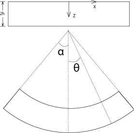
Figure 1: (a) The 2-D view of the reference and current states of the block. (b) Comparison between the plate solution (dashed lines) and exact solution (solid lines) with parameters $\alpha=\pi,\nu=0.3,h=0.1$.

Figure 1 schematically illustrates the 2-D picture of reference and current states of the rectangular block. Cartesian coordinate system $(X,Y,Z)$ is used for a reference point, while cylindrical coordinate system $(\theta,y,r)$ is used for a current point. Then, the bending of the block is described by

$$\theta=\frac{\alpha}{L_{1}}X,\qquad\quad r=r(Z),\qquad\quad y=\lambda_{2}Y,$$ (52)

$$-L_{1}\leq X\leq L_{1},\quad 0\leq Z\leq 2h,\quad-L_{2}\leq Y\leq L_{2},$$

where $\alpha$ is the bending angle, $\lambda_{2}$ is the stretch normal to the bending plane, and $L_{i}$ ($i=1,2$) are the two planar dimensions. Without loss of generality we set $\lambda_{2}=1$ and $L_{1}=1$ ($h$ is then the thickness ratio). The deformation gradient is diagonal in the above coordinate systems

$$\mathbf{F}=\mathrm{diag}[\alpha r,\quad 1,\quad r^{\prime}],$$ (53)

where the prime denotes differentiation with respect to $Z$. As for the constitutive relations, we recall the strain energy for Hill’s class of compressible materials [35],

$$\Phi=\frac{1}{2}\lambda(\mathrm{tr}\mathbf{E}^{(m)})^{2}+\mu\mathrm{tr}[(\mathbf{E}^{(m)})^{2}],\quad\mathbf{E}^{(m)}=\frac{1}{m}\left[(\mathbf{F}^{T}\mathbf{F})^{m/2}-\mathbf{I}\right],$$ (54)

where $\lambda$ and $\mu$ are the Lame constants and $m$ is a parameter running over the reals. The case $m=0$ corresponds to Hencky material, and $m=2$ corresponds to Saint Venant-Kirchhoff material. The nominal stress is given by

$$\mathbf{S}=\mathbf{F}^{-1}\left[\lambda\frac{\mathrm{tr}(\mathbf{V}^{m})-3}{m}\mathbf{V}^{m}+2\mu\frac{\mathbf{V}^{2m}-\mathbf{V}^{m}}{m}\right],\quad\mathbf{V}=\sqrt{\mathbf{F}\mathbf{F}^{T}}.$$ (55)

After some simple algebra, we obtain the following expressions of the two components of the nominal stress ($S_{Yy}$ is not needed)

$$S_{X\theta}=\frac{2\mu(\alpha r)^{m-1}}{1-2\nu}\left[(1-\nu)\frac{(\alpha r)^{m}-1}{m}+\nu\frac{(r^{\prime})^{m}-1}{m}\right],$$ (56)

$$S_{Zr}=\frac{2\mu(r^{\prime})^{m-1}}{1-2\nu}\left[(1-\nu)\frac{(r^{\prime})^{m}-1}{m}+\nu\frac{(\alpha r)^{m}-1}{m}\right],$$

where the parameter $\lambda$ has been replaced by Poisson’s ratio $\nu$ by $\lambda=2\mu\nu/(1-2\nu)$.

For the plate theory, we follow the previous procedure in $(\ref{eq4})$ to expand $r$ in terms of $Z$

$$r(Z)=r_{0}+r_{1}Z+\frac{1}{2}r_{2}Z^{2}+\frac{1}{6}r_{3}Z^{3}+\frac{1}{24}r_{4}Z^{4}+\cdots,\quad 0\leq Z\leq 2h,$$ (57)

where $r_{i}$ ($i=0,..,4$) are the constant coefficients. Accordingly as in $(\ref{eq7},\ref{eq9})$, the deformation gradient and nominal stress are expanded in series of $Z$. As we mentioned earlier, the components $\mathbf{S}^{(i)}$ ($i=0,1,2$) are computed directly from specific form $(\ref{eq57_1})$ by substituting $(\ref{eq58})$ rather than using relations $(\ref{eq10})$. The explicit expressions are given in Appendix B, and the component $\mathbf{S}^{(i)}$ ($i=0,1,2$) depends linearly on the constant $r_{i+1}$. Then, by $(\ref{eq12})$ with $n=0,1$, the constants $r_{i}$ ($i=2,3$) can be expressed by $r_{0}$ and $r_{1}$. For example

$$r_{2}=\frac{-\alpha\bar{r}_{0}^{m-1}r_{1}^{2-m}\left[\bar{r}_{0}^{m}-\left(\bar{r}_{0}^{m}+(m-1)r_{1}^{m}\right)\nu-1\right]}{\nu\bar{r}_{0}^{m}-r_{1}^{m}(\nu-1)+m\left(-\nu\bar{r}_{0}^{m}+2r_{1}^{m}(\nu-1)+1\right)-1},$$ (58)

where $\bar{r}_{0}=\alpha r_{0}$. The expression of $r_{3}$ is given in Appendix B. From the traction condition at $Z=0$ as in $(\ref{eqX1})$, we obtain

$$r_{1}=\left(\frac{\bar{r}_{0}^{m}\nu-1}{\nu-1}\right)^{\frac{1}{m}}.$$ (59)

Finally, the plate equation $(\ref{eq17})_{1}$ furnishes an algebraic equation for $\bar{r}_{0}$ upon using all the recursion relations

$$-3\bar{r}_{0}^{2}\left(\bar{r}_{0}^{m}-1\right)-\frac{3\bar{h}\bar{r}_{0}}{\nu-1}\left(\frac{\bar{r}_{0}^{m}\nu-1}{\nu-1}\right)^{\frac{1}{m}-1}[(2\nu-m(\nu+2)+1)\bar{r}_{0}^{m}$$ (60)

$$+2(m-1)\nu\bar{r}_{0}^{2m}+m-1]+\bar{h}^{2}f_{1}(\bar{r}_{0})=0,$$

where $\bar{h}=\alpha h$ and the explicit expression of $f_{1}$ is omitted. Therefore, the quantity $\bar{r}_{0}$ is a function of the parameter $\bar{h}$ for a fixed $m$. The algebraic equation $(\ref{eq61})$ can be solved numerically without difficulty for any fixed $m$, and for some special values of $m$ analytical solutions are available.

The exact solutions in [33, 34] for the pure bending problem were obtained in integral form , and for some special values of $m$, the integral solution can be reduced to explicit expressions with elementary functions. We can compare the results for any $m$, but in order to see clearly the error we only compare for $m=1$, for which the exact solution and that of our plate equation are both explicit. In our notations the exact solution in [34] takes the form

$$r=r^{\star}(Z)=-\frac{e^{\alpha Z}(1-2\nu)+e^{2\bar{h}}-e^{2\bar{h}-\alpha Z}+1}{\alpha\left(1+e^{2\bar{h}}\right)(\nu-1)},\quad 0\leq Z\leq 2h.$$ (61)

For small thickness ratio $h$, one can do a Taylor expansion. Denoting the corresponding coefficients by $r_{i}^{\star}(i=0,1,2,3)$, we have

$$\bar{r}_{0}^{\star}= \alpha r_{0}^{\star}=1-\bar{h}+\frac{\bar{h}^{3}}{3}+O(\bar{h}^{4}),\quad r_{1}^{\star}=1-\frac{\nu\bar{h}}{\nu-1}+\frac{\nu\bar{h}^{3}}{3(\nu-1)}+O(\bar{h}^{4}),$$ (62)

$$\frac{r_{2}^{\star}}{\alpha}= \frac{\nu}{\nu-1}-\bar{h}+\frac{\bar{h}^{3}}{3}+O(\bar{h}^{4}),\quad\frac{r_{3}^{\star}}{\alpha^{2}}=1-\frac{\nu\bar{h}}{\nu-1}+\frac{\nu\bar{h}^{3}}{3(\nu-1)}+O(\bar{h}^{4}).$$

In the plate theory, for $m=1$ the recursion relations for the coefficients in $(\ref{eq58})$ become

$$r_{1} =\frac{\bar{r}_{0}\nu-1}{\nu-1},\quad r_{2}=-\frac{\alpha(-\nu\bar{r}_{0}+\bar{r}_{0}-1)}{\nu-1},\quad r_{3}=\alpha^{2}r_{1}.$$ (63)

These recursion relations are exact as we mentioned earlier. Indeed, one can check easily that the Taylor expansion coefficients of the exact solution $(\ref{eq62})$ also satisfy these relations. In $(\ref{eq61})$, by setting $m=1$ the equation for $\bar{r}_{0}$ becomes a linear equation, which immediately leads to the solution

$$\bar{r}_{0}=\frac{3-3\bar{h}+2\bar{h}^{2}}{3+2\bar{h}^{2}}.$$ (64)

By further using Taylor expansions in $\bar{h}$, we obtain the first four coefficients in the series of $r$

$$\bar{r}_{0}= 1-\bar{h}+\frac{2\bar{h}^{3}}{3}+O(\bar{h}^{4}),\quad r_{1}=1-\frac{\nu\bar{h}}{\nu-1}+\frac{2\nu\bar{h}^{3}}{3(\nu-1)}+O(\bar{h}^{4}),$$ (65)

$$\frac{r_{2}}{\alpha}= \frac{\nu}{\nu-1}-\bar{h}+\frac{2\bar{h}^{3}}{3}+O(\bar{h}^{4}),\quad\frac{r_{3}}{\alpha^{2}}=1-\frac{\nu\bar{h}}{\nu-1}+\frac{2\nu\bar{h}^{3}}{3(\nu-1)}+O(\bar{h}^{4}).$$

Comparing $(\ref{eq63})$ and $(\ref{eq66})$, one can see that the plate theory yields $O(\bar{h}^{2})$-correct results for $r_{i}$ ($i=0,1,2,3$) (the relative error is of $O(\bar{h}^{3})$). As a result, the current position $r(Z)$, strains and stresses are all pointwise correct up to $O(\bar{h}^{2})$ for all bending angles. This example gives a justification of our plate theory. As far as the authors are aware of, no other plate theory has been shown that it can produce results with a relative error of $O(h^{3})$ for all relevant physical quantities (displacements, strains and stresses) in comparison with the exact solution.

By taking the parameter values $\alpha=\pi,\nu=0.3,h=0.1$, Figure 1 shows the comparison between the plate solution and the exact solution, with an almost indiscernible difference. Actually the maximum relative error is less than $1.5\%$. When $h$ increases to $0.15$, the relative error is $5.1\%$.

Remark: If we use the 2-D plate strain energy function in $(\ref{eq48})$ to deal with this problem, the solution is found to be

$$\bar{r}_{0}= \frac{3(\nu-1)+3(\nu+1)\bar{h}+2(\nu-4)\bar{h}^{2}}{3(\nu-1)+6\nu\bar{h}+8(\nu-1)\bar{h}^{2}}=1-\bar{h}+\frac{8\bar{h}^{3}}{3}+O(\bar{h}^{4}).$$ (66)

Therefore, for the pure bending problem this approach also gives us an $O(h^{2})$- correct solution when the bending angle is prescribed, although the higher-order $O(h^{3})$ terms are different from $(\ref{eq66})_{1}$. Comparing with the above results in $(\ref{eq66})$, the maximum relative error in this approach is increased by about $7$ times. Indeed, in numerical values this energy approach yields relative errors of $10.5\%$ and $36.2\%$ respectively when $h=0.1$ and $h=0.15$.

When the applied bending moment is prescribed, the consistent plate theory can also provide $O(h^{2})$-correct results as the plate boundary condition $(\ref{eq21})$ agrees with this value up to the required order. However, for the energy approach the generalized bending moment (see $(\ref{eq53})_{1})$ has to be assigned this prescribed value. But, it does not conform with the bending moment in the exact formulation, which further induces an $O(h^{2})$ error.

7 Concluding Remarks

In this paper, a finite-strain plate theory, which is term-wise consistent with the 3-D stationary potential energy principle, is developed with no special restrictions on loadings or the order of deformations. It seems that existing plate theories may not enjoy such kind of consistency. The success relies on the derivation of the recursion relations for the coefficients in the series expansion. Another key is to use an expansion for the position vector about the bottom surface, which enables the elimination of the second coefficient exactly. Weak formulations suitable for finite element calculations together with boundary conditions for some practical cases are also provided. Besides the consistency, nice features of this plate theory include: (a) reserving the local force-balance structure in all three directions up to $O(h^{2})$ (in a through-thickness average); (b) obeying a 2-D virtual work principle; (c) not involving unphysical quantities like higher-order stress resultants (usually present in existing higher-order plate theories); (d) when the 3-D edge conditions are known, no need to introduce the so-called generalized traction and generalized bending moment (which do not conform with those in a 3-D formulation); (e) providing up to $O(h^{2})$-correct solution for the pure bending problem of a rectangular block while other plate theories have not been shown to give $O(h^{2})$-correct results in comparison with an exact solution. In some textbook (e.g., [36]), it was asserted that when the thickness ratio is bigger than some value from $\frac{1}{10}$ to $\frac{1}{8}$ plate theories do not apply any more and the 3-D theory should be used. However, for the pure bending problem, our plate theory can actually provide accurate results even when the thickness ratio reaches $0.15$, which breaks the limit in the textbook. Also, in the widely used first-order (Mindlin-Reissner) and third-order shear deformable plate theories for small deflections, there are five differential equations (see [31]), while the present plate theory for finite strains only has three differential equations. So, it appears that the present plate theory is superior to the existing ones.

For the above-mentioned consistency and nice features, a price to pay is that the plate theory cannot be formulated as a 2-D energy minimization problem. By relaxing the consistency a little bit, a 2-D plate strain energy function is obtained by using those recursion relations. Then, a plate problem can be solved through an energy minimization. However, in terms of numerical errors, the consistent plate theory produces a better result than that from this energy approach for the pure bending problem. Another problem in this approach is that the traction and bending moment conditions do not conform with those in the 3-D formulation. We would also like to point out that any plate theory involving generalized traction and generalized bending moment has the same problem. Since they are not equal to the average edge traction and bending moment in the 3-D formulation, one would not expect that an $O(h^{2})$-correct result can be produced. Actually, one can see from $(\ref{eq40})$ that the difference is $O(h^{2})$, and such a difference will lead to an error of $O(h^{2})$ in the solution.

These two types of plate theories raise a philosophical question. Suppose that one plate theory provides an approximation to the governing system satisfied by the minimizer of the 3-D energy functional (like the first theory in this paper) and another plate theory provides a 2-D energy functional which is an approximation to the 3-D energy functional (like the second plate theory). The question is whether the 2-D minimizer in the latter approach approximates the 3-D minimizer to the required order. For example, if one substitute (1.1) into the traction conditions on the top and bottom surfaces, two vector equations for the coefficients are obtained (which the 3-D minimizer should satisfy). Whether the set of equations obtained from the 2-D energy variation (or virtual work principle) for the same coefficients are comparable to these two vector equations (to the required order) is not clear. Based on this reason, a plate theory which directly approximates the governing system for the 3-D minimizer seems to be preferred. Most existing plate theories belong to the 2-D energy approach (in principle), and this might be a reason why so far non plate theories have been shown to achieve $O(h^{2})$-correct (or even $O(h)$-correct) results for all physical quantities.

It is known that so far the method of Gamma convergence fails to provide higher-order (say, $O(h^{2})$) plate theories. Since the present consistent plate theory cannot be formulated as an energy minimization problem, it might hint that the Gamma convergence could not succeed in doing so as it is based on the energy minimization. For direct plate theories, the difficulty is to propose the proper 2-D constitutive relation. The derivations given in this paper indicate that such a relation may not just be the property of the material and plate geometry (see the discussions below $(\ref{eq36})$ and $(\ref{eq48})$ respectively) and depends on the tractions on the bottom/top surfaces as well, which further increases the level of difficulty.

In our derivations, the body force is neglected for simplicity. But, it is a straightforward matter to take it into account. For a dynamic process, the 3-D field equations change to $\mathrm{Div}\mathbf{S}=\rho\ddot{\mathbf{x}}$ with density $\rho$. Correspondingly, the 2-D plate equations become $\nabla\cdot\bar{\mathbf{S}}=\rho\ddot{\bar{\mathbf{x}}}-\bar{\mathbf{q}}$, with some modifications for the intrinsic relations between $\mathbf{x}^{(k)}$ ($k=1,2,3,4$) and $\mathbf{x}^{(0)}$. We shall represent the details elsewhere, together with a study on the degenerated linear plate theory. This work is currently being extended for the derivation of a consistent shell theory.

Finally, we would like to mention that under the imposed smooth assumptions (see, e.g. $(\ref{eq4})$), the plate theory agrees with the 3-D weak formulation to $O(h^{3})$ rigorously and the order of errors in the plate equations and boundary conditions is also rigorous. However, the proof that those errors will lead to an error of the same order for the solution is not provided, which will be left for a future investigation. Plate theories can be dated back at least 150 years ago, and it was stated by Steigmann in [14]: "The derivation of two-dimensional theories of elastic plates from three-dimensional elasticity is one of the main open problems in solid mechanics". In terms of the formal procedure, the agreement with the 3-D weak formulation and the order of error in the field equations and boundary conditions, the present work makes a contribution toward to the resolution of this open problem. Desirably, comparisons between solutions of the present plate theory and those in the 3-D formulation in more numerical examples are needed to see whether this plate theory provides a plausible solution, which will be carried out in the future.

Appendix

Appendix A The differential system from the 2-D plate strain energy

By taking variation of the 2-D plate potential energy in $(\ref{eq48})$ and setting it to be zero, we can obtain

$$\nabla\cdot\hat{\mathbf{S}}=-\bar{\mathbf{q}},\quad in\quad\Omega,$$ (A.1)

$$\mathbf{x}^{(0)}=\mathbf{b}^{(0)}(s),\quad\mathbf{x}^{(1)}=\mathbf{b}^{(1)}(s),\quad on\quad\partial\Omega_{0},$$

$$\hat{\mathbf{S}}^{T}\mathbf{N}=\mathbf{q}_{0},\quad\tilde{\mathbf{S}}^{T}\mathbf{N}=\mathbf{q}_{1},\quad on\quad\partial\Omega_{q}.$$

where the two stress tensors $\hat{\mathbf{S}}$ and $\tilde{\mathbf{S}}$ are expressed as

$$\hat{\mathbf{S}}=\mathbf{S}^{(0)}+h\mathbf{S}^{(1)}+\frac{2}{3}h^{2}\hat{\mathbf{S}}^{(2)}+2h\mathbf{P}_{2},\quad\tilde{\mathbf{S}}=\mathbf{S}^{(0)}+\frac{4h}{3}\mathbf{S}^{(1)}+2h\mathbf{P}_{1},$$ (A.2)

$$\hat{\mathbf{S}}^{(2)}={\mathcal{A}}^{2}[\mathbf{F}^{(1)},\mathbf{F}^{(1)}]-\mathbf{x}^{(2)}\cdot(\nabla\cdot{\mathcal{A}}^{1}),$$

$$\mathbf{p}_{0}=\nabla\cdot\mathbf{S}^{(0)}+\bar{\mathbf{q}},\quad\mathbf{p}_{1}=\mathbf{p}_{0}+\frac{2}{3}h\nabla\cdot\mathbf{S}^{(1)}-\frac{1}{3}h\hat{\mathbf{S}}^{(2)T}\mathbf{k},$$

$$\mathbf{P}_{0}=\frac{\partial\mathbf{B}^{-1}}{\partial\mathbf{F}^{(0)}}[\mathbf{p}_{0}\otimes\mathbf{f}^{(2)}]+{\mathcal{A}}^{2}[\nabla\mathbf{x}^{(1)},\mathbf{B}^{-1}\mathbf{p}_{0}\otimes\mathbf{k}]+\mathbf{B}^{-1}\mathbf{p}_{0}\cdot(\nabla\cdot{\mathcal{A}}^{1}),$$

$$\mathbf{P}_{1}={\mathcal{A}}^{1}[\mathbf{B}^{-1}\mathbf{p}_{0}\otimes\mathbf{k}],\quad\mathbf{P}_{2}={\mathcal{A}}^{1}[\mathbf{B}^{-1}(\mathbf{p}_{1}+h\nabla\cdot\mathbf{P}_{1}-h\mathbf{P}_{0}^{T}\mathbf{k})\otimes\mathbf{k}]+h\mathbf{P}_{0}.$$

The boundary conditions in $(\ref{eq51})$ are parallel to those of cases 1 and 2 of subsection 3(c).

Alternatively, if the variation of the load potential the 2-D energy $\delta\bar{V}_{2D}$ in $(\ref{eq49})$ is used, then the boundary conditions parallel to those in cases 3 to 6 of section 4 will come out. Specifically, the quantities $\bar{\mathbf{S}}$ and $\mathbf{M}$ in $(\ref{eq38}-\ref{eq42})$ are replaced by the newly defined averaged stress $\hat{\mathbf{S}}$ and newly defined moment tensor $\mathbf{\hat{M}}$

$$\mathbf{\hat{M}[N,N]}=h\mathbf{B}_{1}^{T}\mathbf{B}^{-1}\tilde{\mathbf{S}}^{T}\mathbf{N},\quad\mathbf{\hat{M}[N,T]}=h\mathbf{B}_{3}^{T}\mathbf{B}^{-1}\tilde{\mathbf{S}}^{T}\mathbf{N},$$ (A.3)

where $\mathbf{\hat{M}[N,N]}$ is considered as a generalized bending moment.

Note that the explicit expressions for $\hat{\mathbf{S}}$, $\tilde{\mathbf{S}}$ and $\mathbf{\hat{M}}$ in $(\ref{eq52},\ref{eq53})$ are only for comparison with the consistent plate system in section 3. In practice they can be derived directly from the explicit form of $\Phi_{2D}$ in $(\ref{eq48})$. Substituting the relation $(\ref{eq14})$ for $\mathbf{x}^{(2)}$, one can write $\Phi_{2D}=\Phi_{2D}(\nabla\mathbf{x}^{(0)},\mathbf{x}^{(1)},\nabla\mathbf{x}^{(1)})$. Then $\tilde{\mathbf{S}}$ is calculated by

$$\tilde{\mathbf{S}}=\frac{1}{2h^{2}}\frac{\partial\Phi_{2D}}{\partial(\nabla\mathbf{x}^{(1)})}.$$ (A.4)

Further substituting the relation for $\mathbf{x}^{(1)}$, one can write $\Phi_{2D}=\Phi_{2D}(\nabla\mathbf{x}^{(0)},\nabla\nabla\mathbf{x}^{(0)})$. Then $\hat{\mathbf{S}}$ and $\mathbf{\hat{M}}$ are given by

$$\mathbf{M}=\frac{1}{2h}\frac{\partial\Phi_{2D}}{\partial(\nabla\nabla\mathbf{x}^{(0)})},\quad\hat{\mathbf{S}}=\frac{1}{2h}\frac{\partial\Phi_{2D}}{\partial(\nabla\mathbf{x}^{(0)})}-\nabla\cdot\mathbf{M}.$$ (A.5)

Comparing with $(\ref{eq17})$, we see that the present plate equation $(\ref{eq51})_{1}$ does not reserve the force-balance structure inherited from the 3-D system in all three directions. However, as mentioned earlier, with a 2-D plate strain energy function, the plate problem can be considered as an energy minimization problem, which could have advantages in some problems.

Appendix B Some expressions in the pure-bending problem

The components in the series of the nominal stress are given by

$$S_{X\theta}^{(0)}= \frac{2\mu\bar{r}_{0}^{m-1}\left(-\nu r_{1}^{m}+(\nu-1)\bar{r}_{0}^{m}+1\right)}{m(2\nu-1)},\quad S_{Zr}^{(0)}=\frac{2r_{1}^{m-1}\mu\left(-(\nu-1)r_{1}^{m}+\nu\bar{r}_{0}^{m}-1\right)}{m-2m\nu},$$ (B.1)

$$S_{X\theta}^{(1)}= -\frac{2\mu\bar{r}_{0}^{m-2}\left(mr_{2}\nu\bar{r}_{0}r_{1}^{m}-\alpha(2m-1)(\nu-1)\bar{r}_{0}^{m}r_{1}^{2}+\alpha(m-1)\left(r_{1}^{m}\nu-1\right)r_{1}^{2}\right)}{mr_{1}(2\nu-1)},$$

$$S_{Zr}^{(1)}= -\frac{2r_{1}^{m-2}\mu}{m(2\nu-1)\bar{r}_{0}}\left[\alpha mr_{1}^{2}\nu\bar{r}_{0}^{m}+(m-1)r_{2}\nu\bar{r}_{0}^{m+1}\right.$$

$$\left.-r_{2}\left(-(\nu-1)r_{1}^{m}+m\left(2(\nu-1)r_{1}^{m}+1\right)-1\right)\bar{r}_{0}\right],$$

$$S_{X\theta}^{(2)}= \frac{2\mu\bar{r}_{0}^{m-3}}{mr_{1}^{2}(2\nu-1)}\left[-m\left((m-1)r_{2}^{2}+r_{1}r_{3}\right)\nu\bar{r}_{0}^{2}r_{1}^{m}\right.$$

$$\left.+2\alpha^{2}\left(2m^{2}-3m+1\right)(\nu-1)\bar{r}_{0}^{m}r_{1}^{4}-\alpha^{2}\left(m^{2}-3m+2\right)\left(r_{1}^{m}\nu-1\right)r_{1}^{4}\right.$$

$$\left.+\alpha(2m-1)r_{2}(\nu-1)\bar{r}_{0}^{m+1}r_{1}^{2}-\alpha(m-1)r_{2}\left((2m+1)r_{1}^{m}\nu-1\right)\bar{r}_{0}r_{1}^{2}\right],$$

$$S_{Zr}^{(2)}= \frac{2r_{1}^{m-3}\mu}{m(2\nu-1)\bar{r}_{0}^{2}}\left[-\alpha^{2}(m-1)mr_{1}^{4}\nu\bar{r}_{0}^{m}-\alpha m(2m-1)r_{1}^{2}r_{2}\nu\bar{r}_{0}^{m+1}\right.$$

$$-(m-1)\left((m-2)r_{2}^{2}+r_{1}r_{3}\right)\nu\bar{r}_{0}^{m+2}+((m-1)(-2(\nu-1)r_{1}^{m}+mr_{2}^{2}$$

$$\left(4(\nu-1)r_{1}^{m}+1\right)-2)+r_{1}r_{3}\left(-(\nu-1)r_{1}^{m}+m\left(2(\nu-1)r_{1}^{m}+1\right)-1\right))\left.\bar{r}_{0}^{2}\right].$$

The recursion relation for $r_{3}$ is given by

$$r_{3}= \frac{r_{1}^{-m-1}}{\bar{r}_{0}^{2}\left((2m-1)(\nu-1)r_{1}^{m}-(m-1)\nu\bar{r}_{0}^{m}+m-1\right)}\left[-(m-1)r_{2}^{2}\right.$$ (B.2)

$$\left(2(2m-1)(\nu-1)r_{1}^{m}+m-2\right)\bar{r}_{0}^{2}r_{1}^{m}+\alpha^{2}(2m-1)(\nu-1)\bar{r}_{0}^{2m}r_{1}^{4}$$

$$\left.+(m-1)\bar{r}_{0}^{m}\left(r_{2}\nu\bar{r}_{0}\left(2\alpha mr_{1}^{2}+(m-2)r_{2}\bar{r}_{0}\right)r_{1}^{m}+\alpha^{2}\left((m-1)\nu r_{1}^{m}+1\right)r_{1}^{4}\right)\right].$$

References

- [1] Altenbach, H. & Eremeyev, V. A. 2014 actual developments in the nonlinear shell theory– state of the art and new applications of the six-parameter shell theory. Shell structures: Theory and applications, Vol. 3-Pietraszkiewicz and Kreja (eds), pp. 3–12.
- [2] Altenbach, J., Altenbach, H. & Eremeyev, V. A. 2010 On generalized cosserat-type theories of plates and shells: a short review and bibliography. Arch. of Appl. Mech., 80(1), 73–92.
- [3] Kirchhoff, G. 1850 Über das gleichgewicht und die bewegung einer elastischen scheibe. Journal für die reine und angewandte Mathematik, 40, 51–88.
- [4] Love, A. E. H. 1888 The small free vibrations and deformation of a thin elastic shell. Phil. Tran. Royal Soc. Lond. A, pp. 491–546.
- [5] Mindlin, R. D. 1951 Influence of rotary inertia and shear on flexural motions of isotropic, elastic plates. J. of Appl. Mech., 18, 31–38.
- [6] Reddy, J. & Arciniega, R. 2004 Shear deformation plate and shell theories: from stavsky to present. Mech. of Adv. Mater. Struct., 11(6), 535–582.
- [7] Reddy, J. 2007 Theory and analysis of elastic plates and shells. CRC press, Taylor and Francis.
- [8] Von Karman, T. 1910 Festigkeitsprobleme im maschinenbau, vol. 4.
- [9] Kienzler, R. 2002 On consistent plate theories. Arch. Appl. Mech., 72(4-5), 229–247.
- [10] Kienzler, R. & Schneider, P. 2012 Consistent theories of isotropic and anisotropic plates. J. Theor. Appl. Mech., 50, 755–768.
- [11] Reissner, E. 1945 The effect of transverse shear deformation on the bending of elastic plates. J. Appl. Mech., 12, 69–77.
- [12] Reissner, E. 1986 On a mixed variational theorem and on shear deformable plate theory. Inter. J. Numer. Meth. Engi., 23(2), 193–198.
- [13] Meroueh, K. 1986 On a formulation of a nonlinear theory of plates and shells with applications. Comput. Struct., 24(5), 691–705.
- [14] Steigmann, D. J. 2007 Thin-plate theory for large elastic deformations. Inter. J. Non-Linear Mech., 42(2), 233–240.
- [15] Steigmann, D. J. 2013 Koiter’s shell theory from the perspective of three-dimensional nonlinear elasticity. J. Elast., 111(1), 91–107.
- [16] Steigmann, D. J. 2008 Two-dimensional models for the combined bending and stretching of plates and shells based on three-dimensional linear elasticity. Inter. J. Engi. Sci., 46(7), 654–676.
- [17] Steigmann, D. J. 2010 Recent developments in the theory of nonlinearly elastic plates and shells. Shell structures: Theory and applications, Vol. 2-Pietraszkiewicz and Kreja (eds), pp. 19–23, CRC Press, London.
- [18] Ciarlet, P. G. 2005 An introduction to differential geometry with applications to elasticity. Springer, Berlin.
- [19] Le Dret, H. & Raoult, A. 1993 Le modèle de membrane non linéaire comme limite variationnelle de l’élasticité non linéaire tridimensionnelle. Comptes rendus de l’Académie des sciences. Série 1, Mathématique, 317(2), 221–226.
- [20] Le Dret, H. & Raoult, A. 1995 The nonlinear membrane model as variational limit of nonlinear three-dimensional elasticity. J. Math. Pures Appl., 74, 549–578.
- [21] Friesecke, G., James, R. D. & Müller, S. 2006 A hierarchy of plate models derived from nonlinear elasticity by gamma-convergence. Arch. Rational Mech. Analy., 180(2), 183–236.
- [22] Ciarlet, P. G. 1980 A justification of the Von Kármán equations. Arch. Rational Mech. Analy., 73(4), 349–389.
- [23] Erbay, H. 1997 On the asymptotic membrane theory of thin hyperelastic plates. Inter. J. Engi. Sci., 35(2), 151–170.
- [24] Millet, O., Hamdouni, A. & Cimetière, A. 2001 A classification of thin plate models by asymptotic expansion of non-linear three-dimensional equilibrium equations. Inter. J. Non-linear Mech., 36(1), 165–186.
- [25] Dai, H.-H. & Cai, Z. 2006 Phase transitions in a slender cylinder composed of an incompressible elastic material. i. asymptotic model equation. Proc. Royal Soc. Lond. A, 462(2065), 75–95.
- [26] Dai, H.-H. & Wang, F.-F. 2012 Analytical solutions for the post-buckling states of an incompressible hyperelastic layer. Analy. Appl., 10(01), 21–46.
- [27] Dai, H.-H., Wang, Y. & Wang, F.-F. 2013 Primary and secondary bifurcations of a compressible hyperelastic layer: Asymptotic model equations and solutions. Inter. J. Non-Linear Mech., 52, 58–72.
- [28] Dai, H.-H. & Cai, Z. 2012 An analytical study on the instability phenomena during the phase transitions in a thin strip under uniaxial tension. J. Mech. Phy. Solids, 60(4), 691–710.
- [29] Dai, H.-H., Wang, J., Wang, F.-F. & J., X. 2014 Pitchfork and octopus bifurcations in a hyperelastic tube subjected to compression: Analytical post-bifurcation solutions and imperfection sensitivity. to appear in Math. Mech. Solids.
- [30] Ogden, R. 1984 Non-linear elastic deformations. Ellis Horwood, New York.
- [31] Ma, H., Gao, X.-L. & Reddy, J. 2011 A non-classical mindlin plate model based on a modified couple stress theory. Acta Mech., 220(1-4), 217–235.
- [32] Taylor, M., Bertoldi, K. & Steigmann, D. J. 2014 Spatial resolution of wrinkle patterns in thin elastic sheets at finite strain. J. Mech. Phys. Solids, 62(1), 163–180.
- [33] Bruhns, O. T., Xiao, H. & Meyers, A. 2002 Finite bending of a rectangular block of an elastic hencky material. J. Elast. Phys. Sci. Solids, 66(3), 237–256.
- [34] Xiao, H., Yue, Z. & He, L. 2011 Hill s class of compressible elastic materials and finite bending problems: Exact solutions in unified form. Inter. J. Solids Struc., 48(9), 1340–1348.
- [35] Hill, R. 1978 Aspects of invariance in solid mechanics. Adv. Appl. Mech., 18, 1–75.
- [36] Ventsel, E. & Krauthammer, T. 2001 Thin plates and shells: theory: analysis, and applications. CRC press, New York.