The lifetime of cosmic rays in the Milky Way

Abstract

The most reliable method to estimate the residence time of cosmic rays in the Galaxy is based on the study of the suppression, due to decay, of the flux of unstable nuclei such as beryllium–10, that have lifetime of appropriate duration. The Cosmic Ray Isotope Spectrometer (CRIS) collaboration has measured the ratio between the fluxes of beryllium–10 and beryllium–9 in the energy range $E_{0}\simeq 70$–145 MeV/nucleon, and has used the data to estimate an escape time $\tau_{\rm esc}=15.0\pm 1.6$ Myr. This widely quoted result has been obtained in the framework of a simple leaky–box model where the distributions of escape time and age for stable particles in the Galaxy are identical and have exponential form. In general, the escape time and age distributions do not coincide, they are not unique (because they depend on the injection or observation point), and do not have a simple exponential shape. It is therefore necessary to discuss the measurement of the beryllium ratio in a framework that is more general and more realistic than the leaky–box model.

In this work we compute the escape time and age distributions of cosmic rays in the Galaxy in a model based on diffusion that is much more realistic than the simple leaky–box, but that remains sufficiently simple to have exact analytic solutions. Using the age distributions of the model to interpret the measurements of the beryllium–10 suppression, one obtains a cosmic ray residence time that is significantly longer (a factor 2 to 4 depending on the extension of the cosmic ray halo) than the leaky–box estimate. This revised residence time implies a proportional reduction of the power needed to generate the galactic cosmic rays.

1 Introduction

The average residence time of cosmic rays (CR) in the Milky Way is a very important quantity in high energy astrophysics, and is a key element to determine the power required to generate the galactic CR. The most direct way to estimate the average residence time is the measurement of the suppression, due to radioactive decay, of the flux of an unstable nucleus that has a lifetime comparable with the residence time. A longer residence time obviously implies a larger decay probability and a smaller flux. The comparison of the fluxes of two isotopes of the same chemical element, one stable and the other unstable allows to measure the decay suppression for the unstable particle, and the result can then be used to estimate the lifetime of the CR particles.

The most attractive element to perform this program is beryllium that has two stable isotopes (⁷Be and ⁹Be) and one unstable (¹⁰Be) with half–life $1.51\pm 0.04$ Myr [1]. Beryllium is a very rare element in ordinary matter, and essentially all beryllium nuclei in the cosmic rays have not been directly accelerated, but are “secondaries” formed by the fragmentation of heavier nuclei, mostly carbon and oxygen, as they interact with the interstellar gas. This implies that the injection rates for the different isotopes can be calculated from a knowledge of the fluxes of the primary nuclei and of the relevant fragmentation cross sections. More explicitely one can write the injection rate (at the energy per nucleon $E_{0}$ and the space point $\vec{x}$) of the isotope $j$ in the form:

$$q_{j}(E_{0},\vec{x})=n_{\rm ism}(\vec{x})\;\beta\,c\;\sum_{A}n_{A}(E_{0},\vec{x})~{}\sigma_{A}(E_{0})\,B_{j\to A}(E_{0})~{},$$ (1)

where $n_{\rm ism}(\vec{x})$ is the density of the interstellar medium gas, $n_{A}(E_{0},\vec{x})$ is the density of CR nuclei of type $A$ at the same energy per nucleon, $\sigma_{A}$ is the total charge changing cross section for nucleus $A$, and $B_{A\to j}$ the fraction of interactions where a nucleus of type $j$ is produced. The summation is in principle extended to all nuclei of sufficiently large mass, but in practice it is dominated by the contributions of carbon and oxygen. In equation (1) we have also used the (good) approximation that the nuclear fragments emerge from the interaction with the same velocity as the primary nucleus, or equivalently with the same energy per nucleon.

The ratio between the fluxes of beryllium–10 and beryllium–9 at a fixed energy per nucleon (left implicit in the notation) can then be written as the product of three factors:

$$r=\frac{\phi_{10}}{\phi_{9}}=\left\langle P_{\rm surv}\right\rangle\;r_{\sigma}\;r_{\rm prop}=\left\langle P_{\rm surv}\right\rangle~{}\left(\frac{\sum_{A}\phi_{A}\;\sigma_{A}\;B_{A\to 10}}{\sum_{A}\phi_{A}\;\sigma_{A}\;B_{A\to 9}}\right)\;r_{\rm prop}~{}.$$ (2)

In this equation the factor $r_{\sigma}$ is the ratio of the injections for the two isotopes calculated using equation (1) and the assumption that the shape of the energy spectra for the different nuclear types is independent from the space coordinates. The factor $r_{\rm prop}$ takes into account the fact that, even neglecting the effects of decay for beryllium–10, the propagation properties of the two isotopes are not identical. This is because nuclei of the two isotopes with the same energy per nucleon have rigidities that differ by a factor 10/9, and their absorption due to interaction with the interstellar gas are not identical because of small differences in their cross sections. Finally, the factor $\langle P_{\rm surv}\rangle$ takes into account the effect of decay for the flux of the unstable nucleus.

Assuming that the energy of a cosmic ray nucleus remains constant after the injection, and using the notation $f_{\rm age}(t)$ for the (normalized) distribution of the time $t$ elapsed between the instants of injection and observation of a particle, the average survival probability can be calculated as:

$$\left\langle P_{\rm surv}\right\rangle=\int_{0}^{\infty}dt~{}f_{\rm age}(t)~{}e^{-t/T_{\rm dec}}$$ (3)

where $T_{\rm dec}=\tau_{\rm dec}\,\gamma$ is the decay time of the isotope (with $\gamma$ the Lorentz factor of the particles at the energy under study). The distribution $f_{\rm age}(t)$ must be calculated neglecting decay.

Measurements of the beryllium ratio for nuclei with kinetic energy in the interval 70–150 MeV per nucleon have been obtained by different experiments [2, 3, 4], and the results have been used to estimate the CR confinement time. The Cosmic Ray Isotope Spectrometer (CRIS) collaboration aboard the Advanced Composition Explorer spacecraft [4] has measured the beryllium ratio $r=0.123\pm 0.013$, $0.115\pm 0.013$ and $0.122\pm 0.016$ for nuclei in the kinetic energy intervals [70–95], [95-120] and [120–145] MeV/nucleon. The CRIS collaboration has estimated the product $r_{\sigma}\,r_{\rm prop}$ as approximately unity and, interpreting the result on the basis of a steady state leaky–box model, has obtained an “escape time” $\tau_{\rm esc}=15.0\pm 1.6$ Myr. In the leaky–box model the cosmic rays age and escape time distributions are identical and have an exponential form that is determined by the single parameter $\tau_{\rm esc}$ that has the physical meaning of the (position independent) average age and average escape time of the particles.

The cosmic rays “age” and “escape time” are distinct concepts, the first one measures the time elapsed between the instants of injection and observation of a particle, while the second one is the total time that a particle spends in the Galaxy after injection. Accordingly, the age and escape time distributions are in general not identical, and they are also not unique: the age distribution depends on the point of observation, and the escape time distribution depends on the point of injection. It is intuitive that particles injected near the center (periphery) of the Galaxy need a longer (shorter) time to escape, and the average age of the particles observed near (far) from the CR sources is shorter (longer). An interpretation of the observations of beryllium–10 and other unstable nuclei that goes beyond the leaky–box approximation should address these ambiguities. The suppression of the flux of an unstable particle, as shown in equation (3), depends on the age distribution at the observation point.

A fundamental point is that to interpret a measurement of $\langle P_{\rm surv}\rangle$ to obtain information about the cosmic ray residence time (for example to estimate $\langle t_{\rm age}\rangle$ at the solar system position) it is necessary to make some assumption about the shape of the age distribution. The leaky–box hypothesis that the age distribution has a simple exponential form has not a good physical motivation, and uncertainties about the shape of the age distribution, could very well be (see discussion below) the dominant source of error in the estimate of the CR galactic residence time. It is clearly necessary to consider models of the age distributions that are more realistic and have a more robust physical motivation.

In the standard analysis, based on the leaky–box model and used in [2, 3, 4], it is assumed that the age time distribution is a simple exponential:

$$f_{\rm age}(t)=\frac{1}{\langle t_{\rm age}\rangle}e^{-t/\langle t_{\rm age}\rangle}~{}.$$ (4)

The integral in equation (3) can then be easily performed with the result:

$$\left\langle P_{\rm surv}\right\rangle=\frac{1}{1+\langle t_{\rm age}\rangle/T_{\rm dec}}~{}.$$ (5)

Inverting this equation one finds:

$$\frac{\left\langle t_{\rm age}\right\rangle}{T_{\rm dec}}=\frac{1}{\langle P_{\rm surv}\rangle}-1~{}.$$ (6)

Before entering the discussion of how to construct a realistic model for the distribution $f_{\rm age}(t)$ is can be instructive, for a qualitative understanding of how much the estimate of $\langle t_{\rm age}\rangle$ is sensitive to the shape of the distribution, to consider a simple generalization of the exponential distribution of form:

$$f_{\rm age}(t)=\frac{(1+n)^{1+n}}{\Gamma(1+n)}\;\frac{t^{n}}{\langle t_{\rm age}\rangle^{n+1}}\,e^{-t(n+1)/\langle t_{\rm age}\rangle}$$ (7)

(an exponential multiplied by a power law of exponent $n$). This form depends on two parameters, the average age $\langle t_{\rm age}\rangle$ and the adimensional exponent $n$ (that can assume any value in the range $n>-1$). For $n=0$ the distribution function reduces to a simple exponential, for $n<0$ ($n>0$) the distribution has an excess of short (long) times.

Inserting the age distribution (7) in equation (3) one obtains:

$$\langle P_{\rm surv}\rangle=\left(\frac{1+n}{1+n+\langle t_{\rm age}\rangle/T_{\rm dec}}\right)^{1+n}~{},$$ (8)

or inverting

$$\frac{\langle t_{\rm age}\rangle}{T_{\rm dec}}=\frac{1+n}{\langle P_{\rm surv}\rangle^{1/(1+n)}}-(1+n)~{}.$$ (9)

Equations (8) and (9) are the generalizations of (5) and (6) that are recovered for $n=0$. The important point is that the relation between $\langle t_{\rm age}\rangle$, and the survival probability $\langle P_{\rm surv}\rangle$ depends strongly on the parameter $n$. For large $\langle t_{\rm age}\rangle/T_{\rm dec}$) (and small $\langle P_{\rm surv}\rangle$) one has the relation $\langle P_{\rm surv}\rangle\propto\langle t_{\rm age}\rangle^{-(1+n)}$, or $\langle t_{\rm age}\rangle\propto\langle P_{\rm surv}\rangle^{-1/(1+n)}$, that is very sensitive to the value of $n$.

More in general, one can observes that the relation between $\langle t_{\rm age}\rangle$, and $\langle P_{\rm surv}\rangle$, is approximately independent from the shape of the distribution only when $\langle t_{\rm age}\rangle/T_{\rm dec}$ is small and $\langle P_{\rm surv}\rangle$ is close to unity. In fact, developing in series the exponential in equation (3) one can write $\langle P_{\rm surv}\rangle$ as the series:

$$\langle P_{\rm surv}\rangle=1-\frac{\langle t_{\rm age}\rangle}{T_{\rm dec}}+\frac{1}{2}\,\frac{\langle t_{\rm age}^{2}\rangle}{T_{\rm dec}^{2}}+\ldots~{}.$$ (10)

where $\langle t^{k}_{\rm age}\rangle$ is the $k$–th moment of the distribution. When the lifetime of the particles is short (and $\langle P_{\rm surv}\rangle$ is close to unity) one can keep only the first term in the series, and the relation between $\langle P_{\rm surv}\rangle$ and $\langle t_{\rm age}\rangle$ is unique, but in general the dependence of the shape (encoded in the moments $\langle t^{k}_{\rm age}\rangle$) cannot be neglected. In the concrete situation that has emerged from the observations, where the quantity $\langle P_{\rm surv}\rangle$ is of order 0.12, the shape of the residence time distribution is likely to be very important.

In this work we address the problem outlined above, constructing a framework to compute the CR residence and escape time distributions The age distributions can then used to interpret the beryllium ratio measurements. We have tried to construct framework that is much more realistic than the unphysical leaky–box model, but that remains sufficiently simple (it will contains only three parameters) to yield exact analytic expressions for quantities of interest.

The work is organized as follows: in the next section we introduce the simple 1–dimensional diffusion model for propagation in the Galaxy, that is the basis of our calculations, and compute the shape of the escape time distributions (that depends on the particle injection point). In section 3 we compute the age distributions (that are a function of the observation point). In section 4 we compute the average survival probability $\langle P_{\rm surv}\rangle$ and study its relation with the CR lifetime. The final section gives a brief summary and some conclusions.

2 Escape time distribution

Diffusion models are in broad use for the description of the propagation of cosmic rays in the Milky Way (see for example [5, 6]. In this work we will adopt what can be considered as a “minimal” diffusion model, where as the CR galactic confinement volume one takes all space between the parallel planes $z=\pm z_{h}$ (the subscripts stands for halo). These boundary planes are considered as absorption surfaces, and the volume between the planes is considered as filled by a homogeneous diffusive medium, characterized by the isotropic diffusion coefficient $D$.

The assumption of an infinitely large confinement volume is a reasonable approximation if the vertical size of the CR halo $z_{h}$ is much smaller than the galactic radius. The motivation for introducing this approximation is that the calculation of the propagation of cosmic rays is reduced to a 1–dimensional problem that has an exact analytic solution.

In general the diffusion coefficient will be a function of the particle energy (one expects a dependence of form $D=D_{0}(|R|)\beta$, with $R=pc/(Ze)$ the particle rigidity and $\beta$ its velocity), but in this work we will not need to specify the functional form of the energy (or rigidity) dependence of the diffusion coefficient, because we will only discuss the propagation of nuclei, and assume that the energy of the particles remain constant after injection without energy loss or reacceleration. The energy can then be simply considered as a parameter that labels the propagation of different particle types. In most of the following discussion the energy dependence of the different quantities will be left implicit in the notation.

In our framework the only parameter wih the dimension of length is the halo half height $z_{h}$, and by dimensional analysis one can construct only a single independent quantity with the dimension of time, the diffusion time

$$T_{\rm diff}=\frac{z_{h}^{2}}{2\,D}~{}.$$ (11)

The average escape time and age of the cosmic rays (for a fixed energy) will of course be proportional to $T_{\rm diff}$, times adimensional coefficients that will be calculated below.

Neglecting energy loss, but allowing for decay and interaction, the number density $n(\vec{x},t;E)$ of cosmic rays with energy $E$ at the point $\vec{x}$ at the time $t$ can be obtained from the injection rate $q(\vec{x},t;E)$ solving, with appropriate boundary conditions, the partial differential equation:

$$\frac{\partial n(\vec{x},t;E)}{\partial t}=q(\vec{x},t;E)+D(E)\,\nabla^{2}n(\vec{x},t;E)-\frac{n(\vec{x},t;E)}{T_{\rm int}(E)}-\frac{n(\vec{x},t;E)}{T_{\rm dec}(E)}$$ (12)

where $T_{\rm int}$ and $T_{\rm dec}$ are the interaction and decay time of the particle. In equation (12) we have assumed that the interaction rate of a particle is independent from the position $\vec{x}$. This implies that the insterstellar gas density is cosidered homogeneous in the cosmic ray confinement volume. In the following we will neglect the effects of interactions on secondary nuclei. The inclusion, of these effects is straightforward if one makes the hypothesis that the gas distribution is homogeneous, more difficult in the general case.

The general solution of the diffusion equation (12) can be expressed in terms of the Green function $P(\vec{x},\vec{x}_{i},t)$ that gives the probability density that a particle initially at the point $\vec{x}_{i}$ is at the point $\vec{x}$ after a time $t$:

$$n(\vec{x},t_{\rm obs})=\int_{0}^{\infty}dt~{}\int d^{3}x_{i}~{}q(\vec{x}_{i},t_{\rm obs}-t)~{}P(\vec{x},\vec{x}_{i},t)$$ (13)

where $q(\vec{x},t)$ is the number of cosmic rays injected per unit time and unit volume at the point $\vec{x}$ at the time $t$.

Neglecting decay and interactions the Green function can be written explicitely in the form of a series:

$$P_{0}(\vec{x},\vec{x}_{i},t) = \frac{1}{(4\,\pi\,D\,t)^{3/2}}~{}\exp\left[-\frac{(x-x_{i})^{2}+(y-y_{i})^{2}}{4\,D\,t}\right]\times$$

$$\sum_{n=-\infty}^{+\infty}\left\{\exp\left[-\frac{(z-z_{i}-4nz_{h})^{2}}{4\,D\,t}\right]-\exp\left[-\frac{(z+z_{i}-2(2n+1)z_{h})^{2}}{4\,D\,t}\right]\right\}~{}.~{}~{}~{}~{}~{}~{}$$

The function is only defined in the space region $|z|\leq z_{h}$. For $|z|\geq z_{h}$ the particle density and the Green function vanish.

A derivation of equation (2) is simple. For propagation in a homogeneous, isotropic diffusive medium with no boundaries, it is well known that the Green function is a gaussian of width $\sigma^{2}=2\,Dt$. In the presence of the two parallel absorption surfaces at $z=\pm z_{h}$ (see [7]), the Green function becomes the superposition of an infinite number of Gaussian functions all of the same width. One of the gaussians is centered on the real physical source at the point with coordinates $\{x_{i},y_{i},z_{i}\}$, the others correspond to an infinite number of “mirror” sinks and sources placed symmetrically outside the diffusion volume. The sources are located at points $\{x_{i},y_{i},z_{n}^{+}\}$ with:

$$z_{n}^{+}=z_{i}+4\,n\,z_{h}~{},$$ (15)

(the source with $n=0$ is the real physical one). The sinks have coordinates $\{x_{i},y_{i},z_{n}^{-}\}$ with:

$$z_{n}^{-}=-z_{i}+2\,(2n+1)\,z_{h}~{}.$$ (16)

In the presence of interaction and/or decay, the Green function becomes:

$$P(\vec{x},\vec{x}_{i},t)=P_{0}(\vec{x},\vec{x}_{i},t)\;e^{-t/T_{\rm dec}}\;\;e^{-t/T_{\rm int}}~{}.$$ (17)

To compute the escape time distribution one can note that the integral of the Green function $P_{0}$ over the entire Galaxy volume ($|z|\leq z_{h}$):

$${\mathcal{N}}_{0}(t,\vec{x}_{i})=\int d^{3}x~{}P_{0}(\vec{x},\vec{x}_{i},t)$$ (18)

gives a result that is unity for $t=0$ and decreases monotonically with $t$, vanishing for $t\to\infty$. This is the consequence of escape, or formally absorption at the planes $z=\pm z_{h}$

The escape time distribution for a particle that is injected at the point $\vec{x}_{i}$ can then be calculated as:

$$f_{\rm esc}(t,\vec{x}_{i})=-\frac{d{\mathcal{N}}_{0}(t,\vec{x}_{i})}{dt}~{}.$$ (19)

The expression is automatically normalized to unity (for integration in the range $0\leq t<\infty$). The space integration and time derivative in equations (18) and (19) can be easily performed to obtain an explicit expression for $f_{\rm esc}(t)$. Our model is effectively unidimensional, and the escape time distribution depends only on the $z$ coordinate of the injection point, and has a scaling form:

$$f_{\rm esc}(t,\vec{x}_{i})=f_{\rm esc}(t,z_{i})=\frac{1}{T_{\rm diff}}\;F_{\rm esc}\left(\frac{t}{T_{\rm diff}},\frac{z_{i}}{z_{h}}\right)$$ (20)

where $T_{\rm diff}$ is the characteristic diffusion time given in equation (11), and the function $F_{\rm esc}(\tau,x)$ is:

$$F_{\rm esc}(\tau,x) = \frac{1}{2\,\sqrt{2\pi}\,\tau^{3/2}}\;\sum_{n=-\infty}^{+\infty}~{}\left\{e^{-\frac{(x_{n}^{+}+1)^{2}}{2\,\tau}}\,(1+x_{n}^{+})+e^{-\frac{(x_{n}^{+}-1)^{2}}{2\,\tau}}\,(1-x_{n}^{+})\right.$$

$$~{}~{}~{}~{}~{}~{}~{}~{}~{}~{}~{}~{}~{}~{}\left.-e^{-\frac{(x_{n}^{-}+1)^{2}}{2\,\tau}}\,(1+x_{n}^{-})-e^{-\frac{(x_{n}^{-}-1)^{2}}{2\,\tau}}\,(1-x_{n}^{-})\right\}$$

with $x_{n}^{+}=x+4n$ and $x_{n}^{-}=-x+2(2n+1)$. For numerical studies the series in equation (2) converges very rapidly including the first few terms with $|n|$ small.

Examples of the escape time distribution are shown in fig. 1 and fig. 2. Inspecting these figures one can see that for large $t$ ($t/T_{\rm diff}\gg 1$) the distribution approaches asymptotically the exponential form $\propto e^{-t/T^{*}}$ with a slope $T^{*}\simeq 0.810~{}T_{\rm diff}$ that is independent from the injection point. For small $t$ the distribution vanishes, reflecting the fact that the particles need a finite time to reach one of the boundaries of the diffusion volume after injection. The average escape time can be calculated exactly resumming the series, with the result:

$$\left\langle t_{\rm esc}\left(\frac{z_{i}}{z_{h}}\right)\right\rangle=\int_{0}^{\infty}dt~{}t~{}f_{\rm esc}(t,z_{i})=T_{\rm diff}\times\left[1-\frac{z_{i}^{2}}{z_{h}^{2}}\right]$$ (22)

The average escape time is maximum for particles injected in the central plane ($z_{i}=0$), when one has $\langle t_{\rm esc}\rangle=T_{\rm diff}$, and decreases quadratically with $z_{i}$, when the particle is injected closer to one of the boundaries of the Galaxy, vanishing for injection at the boundary of the diffusion volume ($z_{i}=\pm z_{h}$).

3 Residence time Distribution

The age distribution for particles at the point $\vec{x}$ can be obtained from equation (13):

$$f_{\rm age}(t,\vec{x},t_{\rm obs})=\frac{1}{n(\vec{x},t_{\rm obs})}~{}\int d^{3}x_{i}~{}q(\vec{x}_{i},t_{\rm obs}-t)~{}P_{0}(\vec{x},\vec{x}_{i},t)~{}.$$ (23)

The injection rate $q(\vec{x}_{i},t)$ enter in the definition, so the age distribution is determined also by the space and time dependence of the injection.

In the following, in the spirit of constructing simple, exactly solvable models we will consider an injection that is stationary (independent from $t$) and has a very simple space dependence. We will use two models for the injection: the “slab disk”, and the “exponential disk”. In both models the injection depends only on the $z$ coordinate, and is determined by a single parameter (with dimension of length) that gives the spatial thickness of the emission. In the slab disk model the injection is homogeneous in the central region of the halo $|z|<z_{d}$ and vanishes outside:

$$q(z)=\begin{cases}q&{\rm for}~{}~{}|z|\leq z_{d}\\ &{}{}\textstyle\\ 0&{\rm for}~{}~{}|z|>z_{d}~{}.\end{cases}$$ (24)

The parameter $z_{d}$ can take values in the interval $0<z_{d}\leq z_{h}$.

In the exponential disk model the injection has the form

$$q(z)=q_{0}~{}e^{-|z|/z^{*}}~{},$$ (25)

where the parameter $z^{*}$ can take values in the interval $0<z^{*}<\infty$. The two models are identical when their parameters are at the extremes of their intervals of definitions, that is for $z_{d}=z^{*}=0$, when the injection volume is reduced to a plane, and for $z_{d}=z_{h}$ or $z^{*}\to\infty$, when the injection is homogeneous in the entire confinement volume.

It is straightforward to compute the density of cosmic rays for both models. In the slab disk injection model one has:

$$n(z;z_{d})=\frac{q}{D}\;z_{d}~{}z_{h}\times\begin{cases}1-\frac{1}{2}\frac{z_{d}}{z_{h}}-\frac{1}{2}\frac{z^{2}}{z_{d}\;z_{h}}&{\rm for}~{}~{}|z|\leq z_{d}\\ &{}{}\textstyle\\ 1-\frac{1}{2}\frac{|z|}{z_{h}}&{\rm for}~{}~{}|z|>z_{d}~{}.\end{cases}$$ (26)

In the exponential disk injection model:

$$n(z;z^{*})=\frac{q_{0}}{D}\;z^{*}~{}z_{h}\left[1-\frac{|z|}{z_{h}}-\frac{z^{*}}{z_{h}}\;\left(e^{-|z|/z^{*}}-e^{-z_{h}/z^{*}}\right)\right]$$ (27)

In the models the density is proportional to the ratio $q/D$ (or $q_{0}/D$) and only depends on the $z$ coordinate, with a shape determined by the adimensional ratios $z_{d}/z_{h}$ or $z^{*}/z_{h}$, that goes to zero at the boundaries of the confinement volume ($|z|\geq z_{h}$). The $z$ dependence of the CR density is shown in fig. 3 and fig. 4 for the slab and exponential disk models.

The age distribution can be calculated explicitely using equation (23). The result has the same scaling property as the escape time distribution of equation (20):

$$f_{\rm age}(t,\vec{x})=f_{\rm age}(t,z)=\frac{1}{T_{\rm diff}}\;F_{\rm age}\left(\frac{t}{T_{\rm diff}},\frac{z}{z_{h}}\right)$$ (28)

For the slab disk model one obtains:

$$F_{\rm age}(\tau,x;x_{d}) = \frac{1}{2}~{}\sum_{n=-\infty}^{+\infty}~{}\left\{{\rm erf}\left[\frac{x+x_{d}-4n}{\sqrt{2}\,\tau}\right]-{\rm erf}\left[\frac{x-x_{d}-4n}{\sqrt{2}\,\tau}\right]\right.$$

$$~{}~{}~{}~{}~{}~{}~{}~{}~{}~{}~{}\left.+{\rm erf}\left[\frac{x-x_{d}-2(2n+1)}{\sqrt{2}\,\tau}\right]-{\rm erf}\left[\frac{x+x_{d}-2(2n+1)}{\sqrt{2}\,\tau}\right]\right\}$$

where $x=z/z_{h}$, $x_{d}=z_{d}/z_{h}$ and erf indicates the error function.

For the exponential disk model one has:

$$F_{\rm age}(\tau,x;y) = \sum_{n=-\infty}^{+\infty}~{}\left\{e^{\frac{t+8ny2xy}{2y^{2}}}{\rm erf}\left[\frac{t+y+4ny-x\,y}{\sqrt{2\,\tau}\,y}\right]-{\rm erf}\left[\frac{t+4ny-x\,y}{\sqrt{2\,\tau}\,y}\right]\right.$$

$$~{}~{}~{}~{}~{}~{}\left.e^{\frac{t+2(x-4n-2)\,y}{2\,y^{2}}}{\rm erf}\left[\frac{t+y(z-4n-2)}{\sqrt{2\,\tau}\,y}\right]-{\rm erf}\left[\frac{t+y\,(z-4n-1)}{\sqrt{2\,\tau}\,y}\right]\right\}$$

where again $x=z/z_{h}$ and $y=z^{*}/z_{h}$.

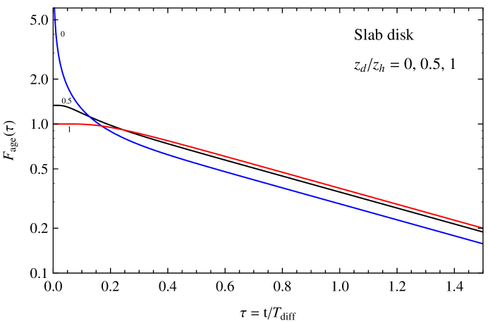
Figure 5: Rescaled age time distribution (see equation (28)). The function is calculated in the slab disk injection model for observations at $z=0$. The different curves correspond to different values of the ratio $z_{d}/z_{h}$ ($z_{d}/z_{h}=0$, 0.5, 1).

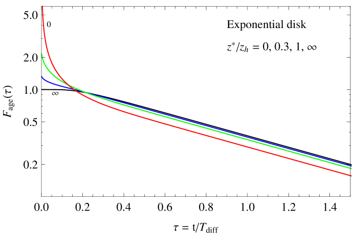
Figure 6: Rescaled age time distribution in the exponential disk model. The different curves correspond to observations at $z=0$ for three different values of the ratio $z^{*}/z_{h}$ ($z^{*}/z_{h}=0$, 0.3, 1, $\infty$).

Examples of the residence time distributions are shown in fig. 5 and fig. 6. In these figures the distributions are shown for an observation point at $z=0$, but for different values of the ratio $z_{d}/z_{h}$ or $z^{*}/z_{h}$. The reason to choose a point at $z\simeq 0$ is that the observations [8] indicate that the solar system lies close (approximately 16 pc) below the galactic plane. Inspecting figures 5 and 6 one can see that the distribution for large $t$ takes an asymptotic exponential form with slope $T^{*}\simeq 0.810~{}T_{\rm diff}$ (the same slope of the escape time distribution at large $t$); for small $t$ the shape deviates from an exponential with, in most cases, an excess at short times. This is the consequence of having a large fraction of the sources at short distances from the observation point. The excess of small $t$ trajectories becomes more important when the ratio between the injection and the confinement volume decreases. In the limit of planar injection ($z_{d}\to 0$ or $z^{*}\to 0$ for the two injection models) the age distribution at small $t$ diverges as $f_{\rm age}(t)\propto 1/\sqrt{t}$.

The average age can be calculated analytically, and the result has a simple form. For slab disk injection model one finds:

$$\left.\frac{\left\langle t_{\rm age}(z,z_{d})\right\rangle}{T_{\rm diff}}\right|_{\rm slab}=\begin{cases}\frac{6x^{2}\,(2-x_{d})-x_{d}\,(8-4x_{d}^{2}+x_{d}^{3})-x^{4}}{6[x^{2}-x_{d}\,(2-x_{d})]}&{\rm for}~{}~{}|z|\leq z_{d}\\ &{}{}\textstyle\\ \frac{2}{3}+\frac{2}{3}\,|x|-\frac{1}{3}\,x^{2}-\frac{1}{3}\,x_{d}^{2}&{\rm for}~{}~{}|z|>z_{d}\end{cases}$$ (31)

(with $x=z/z_{h}$ and $x_{d}=z_{d}/z_{h}$). For the exponential disk injection model:

$$\left.\frac{\left\langle t_{\rm age}(z,z^{*})\right\rangle}{T_{\rm diff}}\right|_{\rm exp}=\frac{e^{\frac{1+x}{y}}(1-x)(2+2x-x^{2}-6y^{2})-3\,e^{x/y}\,y[1-x^{2}-2y^{2}]+6\,e^{1/y}y^{3}}{3\,[e^{\frac{1+x}{y}}(1-x)-e^{\frac{1}{y}}\,y+e^{\frac{x}{y}}\,y]}$$ (32)

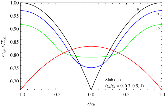
Figure 7: Average CR residence time (or age) calculated in the slab disk injection model, plotted as a function of the ratio $z/z_{h}$. The different curves correspond to three values of the ratio $z_{d}/z_{h}$ ($z_{d}/z_{h}=0$, 0.3, 0.5, 1).

(with $x=z/z_{h}$ and $y=z^{*}/z_{h}$). The average residence time for the two injection models is shown in fig. 7 and fig. 8) plotted as a function of the $z$ coordinate.

In the limiting cases of planar and volume injections one obtains simpler expressions. For planar injection ($z_{d}=0$ or $z^{*}=0$) one has:

$$\left.\frac{\left\langle t_{\rm age}(z)\right\rangle}{T_{\rm diff}}\right|_{\rm plane}=\frac{2}{3}+\frac{2}{3}\,\frac{|z|}{z_{h}}-\frac{1}{3}\,\frac{z^{2}}{z_{h}^{2}}~{}.$$ (33)

For homogeneous injection ($z_{d}=z_{h}$ or $z^{*}\to\infty$):

$$\left.\frac{\left\langle t_{\rm age}(z)\right\rangle}{T_{\rm diff}}\right|_{\rm volume}=\frac{5}{6}-\frac{1}{6}\,\frac{z^{2}}{z_{h}^{2}}$$ (34)

In the first case (injection from a plane) the average CR age is shortest when the observation point is at $z=0$, ($\langle t_{\rm age}\rangle/T_{\rm diff}=2/3$), it grows monotonically with $|z|$, with the maximum at the boundaries of the containement volume at $|z|=z_{h}$, (where $\langle t_{\rm age}\rangle/T_{\rm diff}=1$). For homogeneous injection the situation is reversed, the longest average residence time is at $z=0$ where $\langle t_{\rm age}\rangle/T_{\rm diff}=5/6$; the residence time decreases with $|z|$, with minimum value at the boundaries $\langle t_{\rm age}\rangle/T_{\rm diff}=2/3$.

4 Average survival probability

The quantity $\langle P_{\rm surv}\rangle$ can be calculated from its definition in (3) using the explicit expressions of the age distributions given in equations (3) or (3). The resulting series can be resummed to obtain a simple analytic expression. There is however a much simpler method to obtain $\langle P_{\rm surv}\rangle$, computing the CR density in the entire galactic volume solving equation (12) for an arbitrary value of $T_{\rm dec}$ (or of the combination $T^{-1}=T_{\rm dec}^{-1}+T_{\rm int}^{-1}$), and then taking the ratio with the density calculated for a stable particle (that is $T_{\rm dec}\to\infty$):

$$\langle P_{\rm surv}(\vec{x})\rangle=\frac{n(\vec{x},T)}{n(\vec{x},T\to\infty)}~{}.$$ (35)

For the slab disk injection models the particle density is:

$$n(z,T)=q\;T\times\begin{cases}\left[1-\cosh\left[\frac{z}{\sqrt{D\,T}}\right]\cosh\left[\frac{z_{h}-z_{d}}{\sqrt{D\,T}}\right]\left(\cosh\left[\frac{z_{h}}{\sqrt{D\,T}}\right]\right)^{-1}\right]&{\rm for}~{}~{}|z|\leq z_{d}\\ &{}{}\textstyle\\ \sinh\left[\frac{z_{d}}{\sqrt{D\,T}}\right]\sinh\left[\frac{z_{h}-z}{\sqrt{D\,T}}\right]\left(\cosh\left[\frac{z_{h}}{\sqrt{D\,T}}\right]\right)^{-1}&{\rm for}~{}~{}|z|>z_{d}~{},\end{cases}$$ (36)

For the exponential disk injection model:

$$n(z,T) = \frac{q_{0}\,T\,z^{*}}{(z^{*})^{2}-D\,T}\;\left\{e^{-|z|/z^{*}}\,z^{*}-e^{-z_{h}/z^{*}}\;\cosh\left[\frac{z_{h}}{\sqrt{D\,T}}\right]^{-1}\times\right.$$

$$~{}~{}~{}\;\left.\left(z^{*}\;\cosh\left[\frac{z}{\sqrt{D\,T}}\right]+\sqrt{D\,T}\,e^{z_{h}/z^{*}}\;\sinh\left[\frac{z_{h}-|z|}{\sqrt{D\,T}}\right]\right)\right\}$$

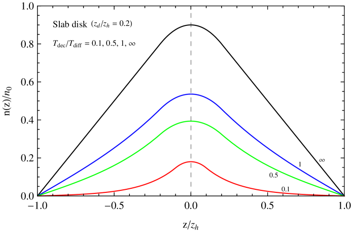
Figure 9: Density of unstable cosmic rays in the slab disk injection model plotted as a function of the ratio $z/z_{h}$. All lines are calculated for a fixed value of the ratio $z_{d}/z_{h}=0.2$. The different curves correspond to stable particles and to unstable particles for a ratio $T_{\rm dec}/T_{\rm diff}=1$, 0.5 and 0.1.

It is straightforward to check that in the limit of $T\to\infty$ one recovers expressions (26) and (27). Examples of the functions $n(z,T)$ for the two injection models are shown in fig. 9 and 10.

It is especially interesting to discuss the average survival probability $\langle P_{\rm surv}\rangle$ at $z=0$ because, as already mentioned, the solar system is close to the galactic plane. For $z=0$, in the slab disk injection model one has:

$$\left\langle P_{\rm surv}(\tau,x_{d})\right\rangle_{\rm slab}=\frac{1-\cosh[\sqrt{2\tau}(1-x_{d})]\;(\cosh[\sqrt{2\tau}])^{-1}}{\tau\,x_{d}(2-x_{d})}~{},$$ (38)

where $\tau=T_{\rm diff}/T_{\rm dec}$ and $x_{d}=z_{d}/z_{h}$. In the exponential disk injection model, for $z=0$ one has:

$$\left\langle P_{\rm surv}(\tau,y)\right\rangle_{\rm exp}=\frac{2y\sqrt{\tau}\;\cosh[\sqrt{2\tau}]^{-1}+e^{1/y}(\sqrt{2}\,\tanh[\sqrt{2\tau}]-2y\sqrt{\tau}}{2\sqrt{\tau}\,[e^{1/y}(1-y)-y)(1-2y^{2}\tau)]}$$ (39)

(with $y=z^{*}/z_{h}$).

Equations (38) and (39) can be seen as the main result of this work, they give average survival probability of an unstable particles as a function of the ratio $T_{\rm diff}/T_{\rm dec}$, for different space distributions of the injection, and different sizes of the confinement volume. The quantity $T_{\rm diff}$ is related to the average escape time $\langle t_{\rm esc}(z_{i})\rangle$ by equation (22) and to the average age $\langle t_{\rm age}(z)\rangle$ by equation (31) or (32).

More in general, the survival probability for observations at a position $z\neq 0$ can be obtained as the ratio of equations (36) and (26), or (4) and (27).

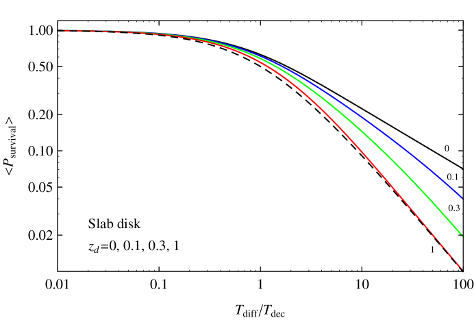
Figure 11: Average survival probability of unstable particles plotted as a function of the ratio $T_{\rm diff}/T_{\rm dec}$. The different curves are calculated in the slab disk model for different values of the parameter $z_{d}/z_{h}$ ($z_{d}/z_{h}=0$, 0.1, 0.3, 1). The dashed line is the leaky–box result plotted as a function of $\langle t_{\rm esc}\rangle/T_{\rm dec}$.

The values of $\langle P_{\rm surv}(\tau)\rangle$ for $\tau$ at the two extremes of its range of definition ($\tau=0$ and $\tau\to\infty$) are are model independent. For $\tau\to 0$ (very short residence time) one has $\langle P_{\rm surv}\rangle=1$, while in the limit $\tau\to\infty$ (very long residence time) one has $\langle P_{\rm surv}\rangle=0$. In general however, the shape of $\langle P_{\rm surv}(\tau)\rangle$ is model dependent. In the two very simple models discussed here the survival probability depends on only one parameter, the ratio $z_{d}/z_{h}$ for the slab disk injection model, or the ratio $z^{*}/z_{h}$ for exponential disk injection. These shapes are shown in figures 11 and 12.

Inspecting the figures one can see that for large $\tau$ the average survival probability decreases as a power law ($\langle P_{\rm surv}\rangle\propto\tau^{-\alpha}$) with an exponent that depends on the ratio $z_{d}/z_{h}$ (or $z^{*}/z_{h}$). In the limiting cases of injection from a plane or from the entire confinement volume one finds (for the observation point at $z=0$):

$$\left\langle P_{\rm surv}(\tau)\right\rangle_{\rm plane}=\frac{\tanh[\sqrt{2\tau}]}{\sqrt{2\tau}}$$ (40)

and

$$\left\langle P_{\rm surv}(\tau)\right\rangle_{\rm volume}=\frac{1}{\tau}\;\left(1-\frac{1}{\cosh[\sqrt{2\tau}]}\right)$$ (41)

These expressions span the entire range of possibilities for the set of models discussed in this work, and for large $\tau$ have the asymptotic behavior:

$$\left\langle P_{\rm surv}(\tau)\right\rangle_{\rm plane}\to\frac{1}{\sqrt{2\tau}}$$ (42)

and

$$\left\langle P_{\rm surv}(\tau)\right\rangle_{\rm volume}\to\frac{1}{\tau}~{}.$$ (43)

More in general, the large $\tau$ behavior of the survival probability ($\langle P_{\rm surv}\rangle\propto\tau^{-\alpha}$) has an exponent $\alpha$ in the interval $1/2\leq\alpha\leq 1$.

The power law behavior of the average survival probability for large $\tau$ can be easily understood qualitatively, as it is related to the shape of the age distribution for small $t$. In the introduction we have shown (see equation (8)) that for an age distribution of form $f_{\rm age}(t)\propto t^{n}\;e^{-t/T}$ (that is $t^{n}$ for small $t$) the survival probability has the asymptotic behavior $\langle P_{\rm surv}\rangle\propto\tau^{-(1+n)}$ (with $\tau=T/T_{\rm dec}$). In the models discussed here, when $t\to 0$ the age distribution $f_{\rm age}(t)$ goes to a constant (that corresponds to $\langle P_{\rm surv}\rangle\propto\tau^{-1}$) for volume injection, and diverges as $t^{-1/2}$ (that results in $\langle P_{\rm surv}\rangle\propto\tau^{-1/2}$) for planar injection.

The different possible functional dependences of $\langle P_{\rm surv}\rangle$ on the ratio $T_{\rm diff}/T_{\rm dec}$ in different models is reflected in a systematic uncertainty in the estimate of the CR residence time, associated to uncertainties in the size of the confinement volume. For $\langle P_{\rm surv}\rangle\lesssim 0.2$, when the use of the asymptotic expressions is a good approximation, one has

$$\left.\frac{\overline{\langle t_{\rm esc}\rangle}}{T_{\rm dec}}\right|_{\rm volume}\simeq\frac{2}{3}\;\frac{1}{\langle P_{\rm surv}\rangle}~{},$$ (44)

for volume injection, and

$$\left.\frac{\overline{\langle t_{\rm esc}\rangle}}{T_{\rm dec}}\right|_{\rm plane}\simeq\frac{1}{2}\;\frac{1}{\langle P_{\rm surv}\rangle^{2}}~{},$$ (45)

for planar injection. In these equations $\overline{\langle t_{\rm esc}\rangle}$ is the particle escape time averaged over all injection points, and have used equation (22) to perform the average over all injection points. For other values of the ratio $z_{d}/z_{h}$ or $z^{*}/z_{h}$, the estimate of the average residence time takes intermediate values between those given in equations (44) and (45).

The estimate $\overline{\langle t_{\rm esc}\rangle}$ for the volume injection given in equation (44) is close to the leaky–box result, but the estimate for planar injection of equation (45) can be much larger. This is illustrated in fig. 13 and 14, that show the interval of $T_{\rm diff}$ that corresponds to the measurement of the beryllium fraction obtained by the CRIS experiment [4] plotted as a function of $z_{d}/z_{h}$ or $z^{*}/z_{h}$ (for the slab disk and exponential disk injection model).

It is virtually certain that the CR sources are in the visible disk of the Galaxy, with a vertical extension of order 0.1–0.15 Kpc. Therefore in good approximation the ratio $z_{d}/z_{h}$ or $z^{*}/z_{h}$ can be interpreted as the inverse of the vertical extension of the CR halo. The observations suggest that the cosmic rays in our Galaxy are confined in a volume that is significantly larger than the visible disk, with a vertical extension of several Kpc. This implies that the leaky–box interpretation of the beryllium isotope ration gives a residence is underestimated by a factor 2 to 4 for a halo half–thickness between 1 and 5 Kpc.

5 Conclusions

The average residence time of cosmic rays in the Milky Way is an important quantity that plays a fundamental role in the estimate of the power of the galactic accelerators. The best method to determine this residence time is the study of the flux of unstable nuclei with a lifetime of appropriate duration.

Measurements of the ratio beryllium–10/beryllium–9 for nuclei with kinetic energy of order 100 MeV/nucleon indicate that the flux of the unstable isotope is suppressed by a factor $\langle P_{\rm surv}\rangle\simeq 0.12$ with respect to to what is expected in the absence of decay. The result clearly shows that the beryllium nuclei have a residence time of the same order of the decay time, but a quantitative estimate requires several assumptions about the propagation of cosmic rays in the Galaxy.

The simplest scheme to interpret the beryllium ratio measurements is the so called leaky–box model that gives [4] an average escape time $15.0\pm 1.6$ Myr. The leaky–box model has the merit of a remarkable simplicity, in fact it can be considered as a “zero–dimension” model where the confinement volume of the cosmic rays is not specified, and the density and injection of the particles are not allowed any dependence on the space coordinates. These unphysical assumptions could (and in fact do) result in a large bias for the estimate of the CR average residence time, and it is clearly very desirable to discuss the problem in models that are more realistic and have a more robust physical motivation.

Some rather elaborate numerical codes like GALPROP [9] or DRAGON [10] have been developed for the study of the propagation of cosmic rays in the Galaxy and can be used to study numerically the confinement of cosmic rays. In this work we have taken the approach of constructing a model that is reasonably realistic, but also sufficiently simple to yield analytic solutions for the quantities of interest, so that the dependence on the model parameters is explicit and transparent, offering a better understanding of the problem.

The framework that we have discussed in this work can be seen as a “minimal” extension of the leaky–box model, and introduces a minimum number (three) of parameters. The framework is a one–dimensional diffusion model, where the Galaxy is an infinite slab of half–thickness $z_{h}$. A second parameter determines the space distribution of the cosmic ray sources (the quantity $z_{d}$ that gives the half–thickness of the injection volume, or alternatively the slope $z^{*}$ for an exponential space distribution of the CR injection). A third parameter (for any given rigidity) is the isotropic diffusion coefficient $D$. The characteristic time for escape from the confinement volume is then $T_{\rm diff}=z_{h}^{2}/(2D)$.

In this simple framework one can compute exactly the escape time and residence time distributions for any possible set of the model parameters. The age and escape time distributions are distinct from each other and are not unique because they depend on the coordinates of the particle injection point (for the escape time) or observation point (for the age time). The average values $\langle t_{\rm esc}(\vec{x}_{i})\rangle$ and $\langle t_{\rm age}(\vec{x})\rangle$ are proportional to $T_{\rm diff}$ times a space–dependent, adimensional coefficient that depends only on the ratio $z_{d}/z_{h}$ or $z^{*}/z_{h}$. The distinction between escape time and age does not exist in the leaky–box model, but is important in a more general discussion of the cosmic ray residence time.

The most interesting result we have obtained is a simple, closed form expression for the average survival probability of an unstable particle $\langle P_{\rm surv}\rangle$ that depends on the $z$ coordinate of the observation point, and is a function of the ratio $T_{\rm diff}/T_{\rm dec}$ (with $T_{\rm dec}$ the decay time of the unstable particle). The crucial point is that $\langle P_{\rm surv}\rangle$ also depends on the ratio $z_{d}/z_{h}$ (or $z^{*}/z_{h}$) between the injection and confinement volumes.

The bottom line is that given a measurement of $\langle P_{\rm surv}\rangle$ that gives the flux suppression for an unstable nucleis, the estimate of the characteristic time $T_{\rm diff}$ (proportional to the average escape time and age of the cosmic rays) depends on the ratio between the injection and confinement volumes for the cosmic rays or, assuming that the injection volume is known, only on the size of the cosmic ray halo.

If the injection and confinement volumes are approximately equal, the relation between $T_{\rm diff}$ and $\langle P_{\rm surv}\rangle$ is very close to what is estimated in the leaky–box model, but when the confinement volume (or $z_{h}$) grows, the estimate of $T_{\rm diff}$ (for a fixed value of $\langle P_{\rm surv}\rangle$) increases monotonically. For a vertical size of the galactic CR halo of order $\simeq 5$ Kpc, the beryllium isotope ratio measurements imply a lifetime of order 50–60 million years, approximately a factor four longer than the leaky–box result. This corresponds to an equal reduction of the power of the galactic CR sources.

Figure 1: Rescaled escape time distribution $F_{\rm esc}(\tau,x)$ (see equation 20)). The three curves correspond to three different injection points ($z_{i}/z_{h}=0$, 0.4, 0.7).

Figure 2: Rescaled escape time distributions $F_{\rm esc}(\tau,x)$ (as in fig. 1). The function is represented in the form $\tau\,F_{\rm esc}(\tau)$ versus $\log\tau$. The area under the curves is unity.

Figure 3: Density of stable cosmic rays in the slab disk injection model plotted as a function of the ratio $z/z_{h}$. The different curves are calculated assuming the same total injection rate and different values of the ratio $z_{d}/z_{h}$ ($z_{d}/z_{h}=0$, 0.3, 0.6, 1).

Figure 4: Density of stable cosmic rays in the exponential disk injection model model plotted as a function of the ratio $z/z_{h}$. The different curves are calculated assuming the same total injection rate and different values of the ratio $z^{*}/z_{h}$ ($z^{*}/z_{h}=0$, 0.2, 0.5, $\infty$).

Figure 8: Average residence time (or age) calculated in the exponential disk injection model, plotted as a function of the ratio $z/z_{h}$. The different curves correspond to three values of the ratio $z^{*}/z_{h}$ ($z^{*}/z_{h}=0$, 0.2, 0.5, $\infty$).

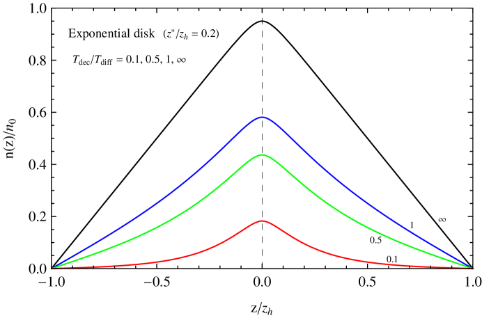
Figure 10: Density of unstable cosmic rays in the exponential disk injection model plotted as a function of the ratio $z/z_{h}$. All lines are calculated for a fixed value of the ratio $z^{*}/z_{h}=0.2$. The different curves correspond to stable particles and to unstable particles for a ratio $T_{\rm dec}/T_{\rm diff}=1$, 0.5 and 0.1.

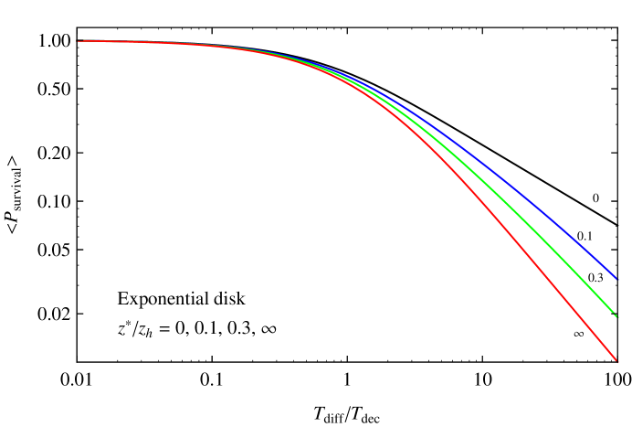
Figure 12: Average survival probability of unstable particles plotted as a function of the ratio $T_{\rm diff}/T_{\rm dec}$. The different curves are calculated in the exponential disk model for different values of the parameter $z^{*}/z_{h}$. ($z^{*}/z_{h}=0$, 0.1, 0.3, $\infty$).

Figure 13: Interval of $T_{\rm diff}$ that corresponds to the average survival probability $\langle P_{\rm surv}\rangle$ obtained by the CRIS experiment [4]. The interval is calculated for the diffusion model discussed in this work with slab disk injection, and is plotted as a function of the ratio $z_{d}/z_{h}$ (the ration between the vertical sizes of the source and confinement volumes). The horizontal band is the estimate of $\langle t_{\rm esc}\rangle$ estimated by the CRIS collaboration in a leaky–box model framework.

Figure 14: As in fig. 13 but the $T_{\rm diff}$ interval is calculated for the exponential disk injection model, and is plotted as a function of the ratio $z^{*}/z_{\rm halo}$.

References

- [1] D. R. Tilley, J. H. Kelley, J. L. Godwin, D. J. Millener, J. E. Purcell, C. G. Sheu and H. R. Weller, Nucl. Phys. A 745, 155 (2004).
- [2] M. Garcia-Munoz, G.M. Mason & J.A. Simpson “The age of the galactic cosmic rays derived from the abundance of Be-10” Astrophys. J. 217, 859 (1977).
- [3] S.P. Ahlen et al. “Measurement of the Isotopic Composition of Cosmic-Ray Helium, Lithium, Beryllium, and Boron up to 1700 MEV per Atomic Mass Unit” Astrophys. J. 534, 757 (2000).
- [4] N.E. Yanasak et al. “Measurement of the Secondary Radionuclides 10Be, 26Al, 36Cl, 54Mn, and 14C and Implications for the Galactic Cosmic-Ray Age” Astrophys. J. 563, 768 (2001).
- [5] V. Ginzburg, V. Dogiel, V. Berezinsky, S. Bulanov, and V. Ptuskin “Astrophysics of Cosmic Rays”, North-Holland, Amsterdam, (1990).
- [6] A. W. Strong, I. V. Moskalenko and V. S. Ptuskin, Ann. Rev. Nucl. Part. Sci. 57, 285 (2007) [astro-ph/0701517].
- [7] D.R. Cox and H.D. Miller, “The Theory of Stochastic Processes”, Chapman and Hall (1965).
- [8] H. T. Freudenreich, Astrophys. J. 492, 495 (1998) [astro-ph/9707340].
- [9] A. E. Vladimirov et al., Comput. Phys. Commun. 182, 1156 (2011) [arXiv:1008.3642 [astro-ph.HE]].
- [10] G. Di Bernardo, C. Evoli, D. Gaggero, D. Grasso and L. Maccione, JCAP 1303, 036 (2013) [arXiv:1210.4546 [astro-ph.HE]].