Half-metallic magnetism and the search for better spin valves

Abstract

We use a previously proposed theory for the temperature dependence of tunneling magnetoresistance to shed light on ongoing efforts to optimize spin valves. First we show that a mechanism in which spin valve performance at finite temperatures is limited by uncorrelated thermal fluctuations of magnetization orientations on opposite sides of a tunnel junction is in good agreement with recent studies of the temperature-dependent magnetoresistance of high quality tunnel junctions with MgO barriers. Using this insight, we propose a simple formula which captures the advantages for spin-valve optimization of using materials with a high spin polarization of Fermi-level tunneling electrons, and of using materials with high ferromagnetic transition temperatures. We conclude that half-metallic ferromagnets can yield better spin-value performance than current elemental transition metal ferromagnet/MgO systems only if their ferromagnetic transition temperatures exceed $\sim$950\text{\,}\mathrm{K}$$.

I Introduction

Magnetic tunnel junctionsJulliere (1975) (MTJs) have attracted considerable attention over the past 20 yearsMoodera et al. (1995); *Miyazaki1995; *Yuasa2004; *Lee2007; *Chappert2007; Parkin et al. (2004) because their use in read headsMoser et al. (2002); *Mao2006; *Mao2007 has improved magnetic memory devices, and because they have potential applications in magnetic switches, magnetic random access memories,Daughton (1997); *Engel2005; *DeBrosse2004 and in spin torqueSlonczewski (1996); *Berger1996; *Slonczewski1989; *Huai2004; *Stiles2006; Hayakawa et al. (2006) and caloritronicWalter et al. (2011); *Lin2012 devices. A MTJ consists of two ferromagnetic layers separated by a tunnel barrier which is normally not magnetic (see Fig. 1). The resistance of a MTJ depends strongly on the relative orientations of the magnetizations of the two ferromagnetic layers. For most applications performance is optimized by achieving the largest possible ambient temperature value of the tunneling magnetoresistance (TMR):

$$\mathrm{TMR}(T)=\frac{G_{P}(T)-G_{A}(T)}{G_{P}(T)}=\frac{R_{A}(T)-R_{P}(T)}{R_{A}(T)}.$$ (1)

Here, $G_{P}(T)$ ($G_{A}(T)$) and $R_{P}(T)$ ($R_{A}(T)$) are the conductances and resistances at temperature $T$ for parallel ($P$) and antiparallel ($A$) magnetization alignments. With this definition a perfect spin-valve, one in which the tunnel current is completely shut-off for $A$ alignment, has $\mathrm{TMR}=1$. In order to achieve a useful device it is important not only that $\mathrm{TMR}(0)$ is close to one, but also that its $\mathrm{TMR}(T)$ does not decrease substantially with increasing $T$ up to the intended operation temperature. In this article we propose a simple formula for the TMR temperature dependence, show that it describes the properties of current high-quality tunnel junctions, and use it to comment on strategies for achieving better MTJs.

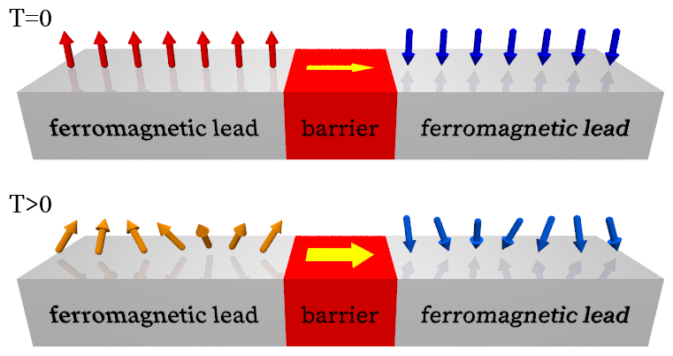
Figure 1: (Color online) Schematic illustration of a magnetic tunnel junction (MTJ). In the high resistance state the magnetizations of the left and right magnetic films at $T=0$ are exactly opposite (top panel) and the exchange potential experienced by transport electrons of a given spin changes sign across the junction. At finite temperature (bottom panel) thermal fluctuations of the left and right magnetizations prevent the layers from maintaining the orientations which maximize the tunnel resistance, allowing a larger current (yellow arrow) to pass through the barrier and reducing the TMR ratio.

II The Stoner Model of $T=0$ TMR

The magnetic and transport properties of most metallic ferromagnets are accurately described at $T=0$ by a mean-field theoryJones and Gunnarsson (1989), typically the Kohn-Sham equations of density functional theory, in which majority and minority spin states experience self-consistently determined spin-dependent potentials. In the following, we use $\downarrow$ to refer to the majority spin orientation on the left side of the tunnel barrier. With this nomenclature, the $\downarrow$ potential is more attractive than the $\uparrow$ potential on both sides of the barrier for $P$ magnetization alignment, whereas for $A$ alignment the $\downarrow$ potential is more attractive on the left side while the $\uparrow$ is more attractive on the right side. When spin-orbit coupling is neglected, $\uparrow$ and $\downarrow$ electrons contribute independently to the conductance in both cases. Because the mean-field Hamiltonians are different, the $\uparrow$ and $\downarrow$ conductances are different in $P$ and $A$ cases, and in the $P$ case also different from each other. Landauer-Büttiker theoryDatta (1997) can be reliably applied to calculate the conductances of accurately characterized tunnel junctions:

$$G_{P} =G^{MM}+G^{mm},$$ (2a)

$$G_{A} =G^{Mm}+G^{mM}=2G^{Mm}.$$ (2b)

Here, the superscript $MM$ refers to majority-spin to majority-spin tunneling, $mm$ to minority-spin to minority-spin tunneling and $Mm$ to majority-spin to minority-spin tunneling. In simplified tunneling Hamiltonian models with spin-independent tunneling amplitudes the conductance contributed by each spin is proportional to the product of its density of states on the two sides of the tunnel barrier, so that $G_{P}\propto\nu_{M}^{2}+\nu_{m}^{2}$, $G_{A}\propto 2\nu_{M}\nu_{m}$, and $\mathrm{TMR}(0)>0$. Although this model never strictly applies to real materials, the TMR nevertheless has a strong tendency to be positive because of the exchange potential jumps across the junction in the $A$ alignment case. The case of half-metallic ferromagnets,Irkhin and Katsnel’son (1994); *Katsnelson2008 in which only majority-spin states or only minority-spin states are present at the Fermi level, provides an extreme example because this property implies that $G^{Mm}=G^{mm}=0$, and hence perfect spin valve behavior with $\mathrm{TMR}(0)=1$.

If the Stoner model captured all relevant physics, the search for optimal spin valves would reduce to a search for half-metallic ferromagnets. Indeed, this search has attracted considerable attention in the spintronics materials community.de Groot et al. (1983); *Hanssen1986; *Hanssen1990; *Weht1999; *Lewis1997; *Kobayashi1998; *Gercsi2006; *Miao2006; *Rybchenko2006; Irkhin and Katsnel’son (1994); *Katsnelson2008 However, remarkably high performance spin valves can still be constructed using materials in which both majority and minority spins are present at the Fermi level. These junctions generally take advantage of the property that majority-spin wave functions of elemental transition-metal ferromagnets decay more slowly than minority-spin wave functions in MgO and other insulating barrier materialsButler et al. (2001), causing the ratio of $G_{P}^{MM}$ to $G_{P}^{mm}$ and $G_{A}^{Mm}$ to grow exponentially with tunnel barrier thickness within the Stoner model. The increase in TMR with barrier thickness is eventually limited by phonon-assisted tunneling and other beyond-Stoner-model effects. It is nevertheless possible to achieve values of $\mathrm{TMR}(0)$ as large as $0.879$ in devices with practical values of the tunnel resistance.Hayakawa et al. (2006)

III TMR at finite temperatures: Theory

As we now explain, uncorrelated thermal fluctuations in magnetization orientation on opposite sides of the tunnel barrier degrade spin-valve performance. This physics is absent in the Stoner model and arises in formal theoretical analyses from the interaction between quasiparticle and spin-wave excitations of the ferromagnets.MacDonald, Jungwirth, and Kasner (1998) It follows that there is a competition in the search for optimal spin valves between choosing materials that are effectively close to being half-metallic and choosing materials that have high ferromagnetic transition temperatures and correspondingly reduced magnetization orientation fluctuations.

Below we propose a simple approximate expression for the finite temperature tunnel magnetoresistance $\mathrm{TMR}(T)$ which depends only on $\mathrm{TMR}(0)$ and on $\zeta(T)=M_{s}(T)/M_{s}(0)$, where $M_{s}(T)$ is the saturation magnetization. In the following, we first present a qualitative discussion which justifies the expression, and then discuss some of its limitations. The expression is motivated by the analysis of the one-particle Green’s function of an itinerant electron ferromagnet presented in Ref. MacDonald, Jungwirth, and Kasner, 1998. As shown there, at non-zero temperatures both majority-spin and minority-spin Green’s functions have poles at both minority-spin and majority-spin quasiparticle energies. Provided that the quasiparticle exchange splitting is larger than spin-wave energies, and that the temperature is low enough that only long-wavelength spin waves are thermally excited, the residue of the majority-spin Green’s function is $(1+\zeta(T))/2$ at majority-spin quasiparticle poles and $(1-\zeta(T))/2$ at minority-spin quasiparticles poles. Similarly, the residue of the minority-spin Green’s function is $(1-\zeta(T))/2$ at majority-spin quasiparticle poles and $(1+\zeta(T))/2$ at minority-spin quasiparticles poles. The interpretation of these theoretical results is straight forward. Because of thermal fluctuations in magnetization orientation an electron with a given definite spin has a finite probability at finite temperature of being a majority-spin electron and a finite probability of being a minority-spin electron.

When these temperature-dependent quasiparticle weights are included, many of the deficiencies of the Stoner theory of itinerant electron magnetism are repaired. In particular, it is no longer difficult to reconcile the temperature dependence of the magnetization, which is controlled by long-wavelength thermally excited magnons whose occupation numbers are given by the Bose distribution function, with the temperature dependence of electron quasiparticle occupation numbers that are given by the Fermi distribution function. In addition, we can repair the theory of TMR by adding the independent conductivities contributed by the two average spin orientations and in each case assigning probabilities for instantaneous spin orientations on each side of the junction. For example, the majority-spin conductivity in the $P$ alignment case is

$$G^{MM}(T)=\lambda(T)\biggl{[}G^{MM}\biggl{(}\frac{1+\zeta(T)}{2}\biggr{)}^{2}+G^{mm}\biggl{(}\frac{1-\zeta(T)}{2}\biggr{)}^{2}+2G^{Mm}\biggl{(}\frac{1+\zeta(T)}{2}\biggr{)}\biggl{(}\frac{1-\zeta(T)}{2}\biggr{)}\biggr{]}.$$ (3)

This approximation leads to

$$G_{P,A}(T)=\lambda(T)\biggl{[}(G^{MM}+G^{mm})\biggl{(}\frac{1\pm\zeta(T)^{2}}{2}\biggr{)}+2G^{Mm}\biggl{(}\frac{1\mp\zeta(T)^{2}}{2}\biggr{)}\biggr{]}=\frac{\lambda(T)}{2}\bigl{[}G_{P}\bigl{(}1\pm\zeta(T)^{2}\bigr{)}+G_{A}\bigl{(}1\mp\zeta(T)^{2}\bigr{)}\bigr{]},$$ (4)

where the upper (lower) sign refers to the $P$ ($A$) alignment case. Hence we find that

$$\mathrm{TMR}(T)=\mathrm{TMR}(0)\frac{\zeta(T)^{2}}{1-\mathrm{TMR}(0)(1-\zeta(T)^{2})/2}.$$ (5)

The factor of $\lambda(T)$ in Eqs. (3) and (4) accounts for the Fowler-NordheimFowler and Nordheim (1928); *Nordheim1928; Forbes (2004); *Forbes2008 thermal smearing effects responsible for the temperature dependence of tunneling conductances in non-magnetic systems. At low temperature, $\lambda(T)$ usually increases quadratically with increasing temperature (see App. A). Note that with these definitions $\lambda(0)=\zeta(0)=1$. In Fig. 2 we plot $\mathrm{TMR}(T=$300\text{\,}\mathrm{K}$)$ as a function of $\mathrm{TMR}(0)$ and the ferromagnetic critical temperature $T_{c}$ by assuming that $\zeta(T)=1-(T/T_{c})^{3/2}$ to interpolate the dependence of magnetization between low temperature and the Curie temperature. Based on this plot we conclude that in searching for optimal spin-valve behavior a very high ferromagnetic transition temperature is at least as important as good low-temperature spin-valve behavior.

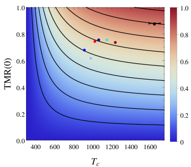
Figure 2: (Color online) Color-scale plot of $\mathrm{TMR}(T=$300\text{\,}\mathrm{K}$)$ as a function of $\mathrm{TMR}(0)$ and the ferromagnetic critical temperature $T_{c}$ assuming that $\zeta(T)=1-(T/T_{c})^{3/2}$. The solid lines are contours of constant $\mathrm{TMR}(T)$ separated in value by $0.1$. The symbols plot the $\mathrm{TMR}_{\mathrm{fit}}($300\text{\,}\mathrm{K}$)$ values of Tab. 1 using the same color code as in Fig. 3. All data points reported as being measured on the same sample are represented by the same color throughout this paper. The error bars represent uncertainties in determining values from published figures.

Eq. (5) becomes exactMacDonald, Jungwirth, and Kasner (1998) when (i) there are no exchange interactions and therefore no correlations between magnetization orientations across the tunnel barrier, (ii) Boltzmann weighting factors are large only for magnetization configurations in which orientations change slowly on a lattice constant length scale, (iii) thermal fluctuations at the interfaces between nanomagnets and tunnel barriers are similar to those of bulk magnetic material, and (iv) the tunneling amplitude across the barrier is spin-independent. Among these four conditions the first two are normally safely satisfied. Because magnetization fluctuations are typically larger at surfaces of nanomagnets or at interfaces with non-magnetic materials, the factor $\zeta(T)$ in Eq. (5) should likely be chosen to be smaller than the bulk magnetization thermal suppression factor, enhancing the importance of a high Curie temperature in achieving good spin valves. The fourth requirement for Eq. (5) is the most seriously violated in most TMR systems. For example, spin-dependent tunneling figures prominently in yielding the very large value of $\mathrm{TMR}(0)$ in FeCo/MgO TMR systems.Butler et al. (2001) Conceptually, $\mathrm{TMR}(T)$ should be performing a Boltzmann-weighted average of TMR values calculated for all realized magnetization configurations. Most configurations have substantial non-collinearity particularly inside the tunnel barrier. The main effect of thermal fluctuations is that non-collinearity increases $G_{A}$, and thus reduces the TMR. The property that the typical degree of local non-collinearity is greater in materials with lower magnetic transition temperatures is captured by Eq. (5). The reliability of this equation is discussed further below.

IV TMR at finite temperatures: Experiment

We have compared recent TMR measurement reportsParkin et al. (2004); Hayakawa et al. (2006); Wang et al. (2008); Ma et al. (2009) which contains values for both $G_{P}(T)$ and $G_{A}(T)$ (or equivalently $R_{P}(T)$ and $R_{A}(T)$ or the corresponding resistance-area products) with Eq. (4), forcing agreement by fixing the values of $\lambda(T)$ and $\zeta(T)$:

$$\zeta^{2}(T) =\frac{G_{P}(T)-G_{A}(T)}{G_{P}(T)+G_{A}(T)}\biggr{/}\frac{G_{P}^{0}-G_{A}^{0}}{G_{P}^{0}+G_{A}^{0}},$$ (6a)

$$\lambda(T) =(G_{P}(T)+G_{A}(T))/(G_{P}^{0}+G_{A}^{0}).$$ (6b)

In Fig. 3 we plot experimental data from Refs. 7; 19 (top row) and Refs. 41; 42 (bottom row). In Refs. 7; 19 the authors analyzed sputter-deposited CoFe(B)/MgO/CoFe(B) MTJs, whereas in Refs. 41; 42 the authors analyzed epitaxial MBE-grown Fe/MgO/Fe junctions. In all these studies, the MgO tunnel barrier was oriented along (100). Fig. 3 presents fits of this data to Eq. (4) using $T=0$ conductance and TMR values, and $T_{c}$ along with a characteristic Fowler-Nordheim tunneling temperature scale $T_{FN}$ as fitting parameters (for details see App. A). A summary of the MTJ sample geometries, key data values, and the parameters obtained by fitting the TMR data is given in Tab 1. As seen in Fig. 3, the fits generally describe the temperature dependence of the data well and are most accurate for the MBE-grown Fe/MgO/Fe samples.

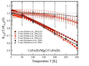
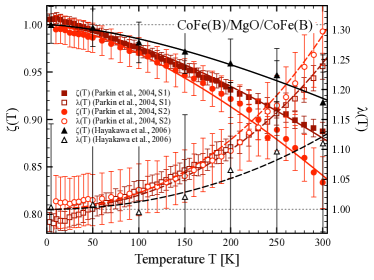
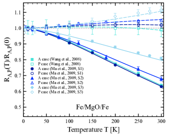
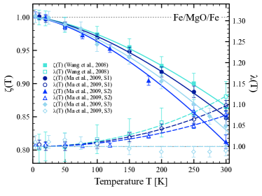
Figure 3: (Color online) Left column: $R_{P}(T)$ and $R_{A}(T)$ normalized to their zero-temperature values for the samples studies in Refs. 7; 19; 41; 42 compared with the fitting formulas proposed in this paper. Right column: $\zeta(T)$ (left axis) and $\lambda(T)$ (right axis) fits. $G_{P}(T)+G_{A}(T)$ increases with temperature in a manner similar to typical behavior for tunneling between non-magnetic metals. At the same time $\mathrm{TMR}(T)$ decreases as thermal fluctuations reduce the dependence of conductance on mean magnetization orientations. The end result is that $R_{P}(T)$ ($R_{A}(T)$) is more weakly (strongly) temperature dependent than in normal metals. The error bars in these plots represent uncertainties in determining values from published figures.

Ref./Sample	MTJ structure	$T_{c}^{\mathrm{eff}}$ [K]	$\mathrm{TMR}_{\mathrm{fit}}(0)$	$\mathrm{TMR}_{\mathrm{fit}}($300\text{\,}\mathrm{K}$)$	$\mathrm{TMR}_{\mathrm{exp}}($300\text{\,}\mathrm{K}$)$
Parkin et al., 2004, S1	3.0 Co70Fe30/2.9 MgO/15.0 Co84Fe16	$1235\,\pm\,11$	$0.742\,\pm\,0.001$	$0.627\,\pm\,0.001$	$0.635\,\pm\,0.006$
Parkin et al., 2004, S2	3.0 Co70Fe30/3.1 MgO/15.0 Co84Fe16	$1022\,\pm\,14$	$0.749\,\pm\,0.002$	$0.595\,\pm\,0.002$	$0.590\,\pm\,0.06$
Hayakawa et al., 2006	3.0 Co40Fe40B20/1.5 MgO/3.0 Co40Fe40B20	$1647\,\pm\,58$	$0.879\,\pm\,0.003$	$0.800\,\pm\,0.003$	$0.81\,\pm\,0.02$
Wang et al. 2008	25.0 Fe/3.0 MgO/10.0 Fe	$1146\,\pm\,10$	$0.761\,\pm\,0.001$	$0.631\,\pm\,0.001$	$0.63\,\pm\,0.02$
Ma et al., 2009, S1	25.0 Fe/3.0 MgO/10.0 Fe	$1061\,\pm\,9$	$0.761\,\pm\,0.001$	$0.614\,\pm\,0.001$	$0.630\,\pm\,0.005$
Ma et al., 2009, S2	25.0 Fe/2.1 MgO/10.0 Fe	$910\,\pm\,13$	$0.684\,\pm\,0.002$	$0.509\,\pm\,0.002$	$0.512\,\pm\,0.008$
Ma et al., 2009, S3	25.0 Fe/1.5 MgO/10.0 Fe	$978\,\pm\,14$	$0.622\,\pm\,0.002$	$0.474\,\pm\,0.002$	$0.477\,\pm\,0.009$

Table 1: Comparison of experimental room temperature TMR data from Refs. 7; 19; 41; 42 to our theory, Eq. (5). The stack layer thicknesses are in nm units. The errors stem from uncertainties in determining values from published figures.

It is important to observe that there are data in the literature which are not well described by our theory. One example are the observations reported in Ref. 43, summarized in Fig. 4, which studied 30 Mn_xGa_100-x/$\mathrm{t}_{\mathrm{CoFeB}}$CoFeB/0.4 Mg/2.2 MgO/0.2 Mg/1.2 CoFeB MTJ stacks. The thickness $\mathrm{t}_{\mathrm{CoFeB}}$ of the CoFeB layer adjacent to the (Mn,Ga) was varied between $0$ and $1.5\text{\,}\mathrm{nm}$. Our theory completely fails to describe the two samples with $\mathrm{t}_{\mathrm{CoFeB}}=$0\text{\,}\mathrm{nm}$$ and $\mathrm{t}_{\mathrm{CoFeB}}=$1.0\text{\,}\mathrm{nm}$$ for which the influence of the Mn_xGa_100-x layer is largest. The authors state that Mn atoms in these samples diffuse into the MgO layer. It seems likely that the Mn atoms induce local moments in the MgO that are detrimental for TMR and lie outside the physics that our approximate formula aims to capture. For the sample in this series with the thickest CoFeB, $\mathrm{t}_{\mathrm{CoFeB}}=$1.5\text{\,}\mathrm{nm}$$, curves in Fig. 4 are more similar to those in Fig. 3 above about $100\text{\,}\mathrm{K}$.

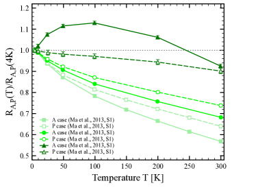
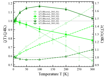
Figure 4: (Color online) Left panel: $P$ and $A$ resistances vs. temperature for the data of Ref. 43. Right panel: $\zeta(T)$ (left axis) and $\lambda(T)$ (right axis) calculated from the data using Eq. (6) and normalized to their values at $T=$4\text{\,}\mathrm{K}$$. For sample S1: $\mathrm{t}_{\mathrm{CoFeB}}=$0\text{\,}\mathrm{nm}$$, S2: $\mathrm{t}_{\mathrm{CoFeB}}=$1.0\text{\,}\mathrm{nm}$$, S3: $\mathrm{t}_{\mathrm{CoFeB}}=$1.5\text{\,}\mathrm{nm}$$. The error bars represent uncertainties in determining values from published figures.

V Summary and Conclusions

We have proposed a simple formula, Eq. (5), for the temperature-dependent TMR of a MTJ. Eq. (5) captures the property that the effectiveness of a tunnel-junction spin-valve depends both on the way in which spin-dependent exchange potentials influence the transport properties of electronic quasiparticles driven through a tunnel junction by a bias voltage, and on the degree to which those exchange potentials thermally fluctuate around mean values which can be controlled experimentally. The physics which controls the value of the TMR at $T=0$ depends mainly on electronic structure considerations in magnetic materials which are often accurately described by spin-density functional theory. For specific material combinations $\mathrm{TMR}(0)$ can be calculated accurately by separately evaluating the tunnel conductances of $P$ and $A$ magnetization configurations using the Landauer-Büttiker formulaDatta (1997) and the Green’s function methods of nanoelectronics. $\mathrm{TMR}(0)$ reaches its maximum value when either only majority or only minority spins are present at the Fermi level, i.e. in the case of half-metallic ferromagnetism. However, for sufficiently thick barriers quite large values of $\mathrm{TMR}(0)$ can still be achieved when both minority and majority spins have substantial presence at the Fermi energy, provided that the wave functions of one or the other decay more slowly in the tunnel barrier. At finite temperatures electronic structure theory considerations do not capture the most important source of TMR temperature dependence, uncorrelated thermal fluctuations in magnetization orientation on opposite sides of the tunnel barrier. This effect is captured in a very simple way in Eq. (5), where $\mathrm{TMR}(T)$ is related to the degree to which thermal fluctuations reduce the magnetization close to the tunnel barrier, $\zeta(T)=M_{s}(T)/M_{s}(0)$. In order to interpret literature experimental data using Eq. (5), we have assumed that in any viable spin-valve system we can use the low-temperature expression $\zeta(T)=1-(T/T_{c})^{3/2}$ for $\zeta(T)$. The $T_{c}$ values we obtain by fitting literature TMR data to Eq. (5), listed in Tab. 1, should be understood not literally as ferromagnetic critical temperature values, but as a number which characterizes the relative strength of thermal fluctuation effects in particular MTJ systems. The fact that the TMR fitting temperatures are nevertheless in each case comparable to the true ferromagnetic critical temperatures associated with the employed materials ($T_{c}\sim$1040\text{\,}\mathrm{K}$$ in bulk Fe, $\sim$1400\text{\,}\mathrm{K}$$ in bulk Co), provides strong evidence that we have correctly identified the origin of temperature dependence. In the light of this agreement, we are confident that Eq. (5) can be used to estimate the room temperature TMR of high-quality spin-valve systems given only their $\mathrm{TMR}(0)$ and the magnetic critical temperature of its magnetic constituents (see Fig. 2). We can therefore conclude that the room temperature TMR values of spin-valves fabricated with half-metallic magnetic materials can exceed those of existing spin-valves fabricated with Fe, Co, CoFeB, and similar magnetic materials combined with MgO tunnel barriers only if the half-magnetic material has a critical temperature exceeding at least $\sim$900\text{\,}\mathrm{K}$$. The highest reported room temperature TMR value with standard materials is $\sim 0.81$ (Ref. 19). According to Eq. (5), this value is achieved for $\mathrm{TMR}(0)=1$ if $\zeta($300\text{\,}\mathrm{K}$)=0.825$ which corresponds to $T_{c}^{\mathrm{eff}}=$960\text{\,}\mathrm{K}$$. These considerations rule clearly out most known half-metallic magnetic materials, with ferrimagnetic Fe₃O₄ ($T_{c}=$858\text{\,}\mathrm{K}$$) standing out as a notable exception.

Appendix A Fitting procedure

We extracted resistance (or resistance-area product) data $R_{A,P}(T)$ from Refs. 7; 19; 41; 42. Starting from Eq. (4) in the main text, we can express $\zeta(T)$ and $\lambda(T)$ in terms of the measured resistances using

$$\zeta^{2}(T) =\frac{R_{A}(T)-R_{P}(T)}{R_{A}(T)+R_{P}(T)}\biggr{/}\frac{R_{A}(0)-R_{P}(0)}{R_{A}(0)+R_{P}(0)},$$ (7a)

$$\lambda(T) =\frac{R_{A}(T)+R_{P}(T)}{R_{A}(T)R_{P}(T)}\biggr{/}\frac{R_{A}(0)+R_{P}(0)}{R_{A}(0)R_{P}(0)}$$ (7b)

with $\lambda(0)=\zeta(0)=1$. As discussed in the main text, we expect the temperature dependence of the saturation magnetization behaviour to fall off in temperature as $\zeta(T)=1-(T/T_{c}^{\mathrm{eff}})^{3/2}$ for $T<T_{c}^{\mathrm{eff}}$ and fit results at all temperatures using a single parameter $T_{c}^{\mathrm{eff}}$ which reflects the strength of thermal magnetization fluctuations in the MTJ device. $\lambda(T)$ accounts for the Fowler-Nordheim thermal smearing effectsFowler and Nordheim (1928); *Nordheim1928; Forbes (2004); *Forbes2008 and is commonly modeled using $\lambda(T)=[(T/T_{\mathrm{FN}})/\sin(T/T_{\mathrm{FN}})]\approx 1+(T/T_{\mathrm{FN}})^{2}/6$, where we have introduced a Fowler-Nordheim temperature $T_{\mathrm{FN}}$ defined by $T_{\mathrm{FN}}=d_{F}/(\pi k_{B})$. $d_{F}$ is the barrier decay length expressed in energy units and can be directly related to the barrier height.Forbes (2004, 2008) We have used one parameter $T_{FN}$ to fit the measured resistances at all temperatures.

Because zero-temperature data are not always available we have found it convenient to perform instead a closely related four-parameter fit of the temperature-dependent $P$ and $A$ resistances by defining

$$\tilde{\zeta}(T) =\biggl{(}\frac{R_{A}(T)-R_{P}(T)}{R_{A}(T)+R_{P}(T)}\biggr{)}^{1/2},$$ (8a)

$$\tilde{\lambda}(T) =\frac{R_{A}(T)+R_{P}(T)}{R_{A}(T)R_{P}(T)},$$ (8b)

and fitting measured values to the following functions:

$$\tilde{\zeta}(T) =\tilde{\zeta}_{0}\bigl{[}1-(T/T_{c}^{\mathrm{eff}})^{3/2}\bigr{]},$$ (9a)

$$\tilde{\lambda}(T) =\tilde{\lambda}_{0}\bigl{[}(T/T_{\mathrm{FN}})/\sin(T/T_{\mathrm{FN}})\bigr{]}.$$ (9b)

The values of the four parameters $T_{c}^{\mathrm{eff}},T_{\mathrm{FN}},\tilde{\zeta}_{0},\tilde{\lambda}_{0}$ which provide the best fits to the data shown in Fig. 3 are listed in Tab. 2. From these fit parameters we obtain $\mathrm{TMR}(0)$ using:

$$R_{P,A}(0) =2/[\tilde{\lambda}_{0}(1\pm\tilde{\zeta}_{0}^{2})],$$ (10a)

$$\mathrm{TMR}(0) =2\tilde{\zeta}_{0}^{2}/(1+\tilde{\zeta}_{0}^{2}).$$ (10b)

Ref./Sample	$T_{c}^{\mathrm{eff}}$ [K]	$T_{FN}$ [K]	$\tilde{\zeta}_{0}$	$\tilde{\lambda}_{0}$ [$\Omega^{-1}$]
Parkin et al., 2004, S1	1235	268	0.768	$6.55\cdot 10^{-3}$
Parkin et al., 2004, S2	1022	249	0.774	$1.655\cdot 10^{-2}$
Hayakawa et al., 2006	1647	366	0.885	$2.90$
Wang et al. 2008	1146	367	0.784	$3.781\cdot 10^{-5}$
Ma et al., 2009, S1	1061	406	0.784	$7.83\cdot 10^{-7}$
Ma et al., 2009, S2	910	459	0.721	$7.58\cdot 10^{-5}$
Ma et al., 2009, S3	978	$\infty$	0.672	$1.129\cdot 10^{-3}$

Table 2: Fit parameters for data from Refs. 7; 19; 41; 42.

References

- Julliere (1975) M. Julliere, Phys. Lett. A 54, 225 (1975).
- Moodera et al. (1995) J. S. Moodera, L. R. Kinder, T. M. Wong, and R. Meservey, Phys. Rev. Lett. 74, 3273 (1995).
- Miyazaki and Tezuka (1995) T. Miyazaki and N. Tezuka, J. Magn. Magn. Mat. 139, L231 (1995).
- Yuasa et al. (2004) S. Yuasa, T. Nagahama, A. Fukushima, Y. Suzuki, and K. Ando, Nat. Mater. 3, 868 (2004).
- Lee et al. (2007) Y. M. Lee, J. Hayakawa, S. Ikeda, F. Matsukura, and H. Ohno, Appl. Phys. Lett. 90, 212507 (2007).
- Chappert, Fert, and Van Dau (2007) C. Chappert, A. Fert, and F. N. Van Dau, Nat. Mater. 6, 813 (2007).
- Parkin et al. (2004) S. S. P. Parkin, C. Kaiser, A. Panchula, P. M. Rice, B. Hughes, M. Samant, and S.-H. Yang, Nat. Mater. 3, 862 (2004).
- Moser et al. (2002) A. Moser, K. Takano, D. T. Margulies, M. Albrecht, Y. Sonobe, Y. Ikeda, S. Sun, and E. E. Fullerton, J. Phys. D Appl. Phys. 35, R157 (2002).
- Mao et al. (2006) S. Mao, Y. Chen, F. Liu, X. Chen, B. Xu, P. Lu, M. Patwari, H. Xi, C. Chang, B. Miller, D. Menard, B. Pant, J. Loven, K. Duxstad, S. Li, Z. Zhang, A. Johnston, R. Lamberton, M. Gubbins, T. McLaughlin, J. Gadbois, J. Ding, B. Cross, S. Xue, and P. Ryan, IEEE T. Magn. 42, 97 (2006).
- Mao (2007) S. Mao, J. Nanosci. Nanotechnol. 7, 1 (2007).
- Daughton (1997) J. M. Daughton, J Appl Phys 81, 3758 (1997).
- Engel et al. (2005) B. N. Engel, J. Akerman, B. Butcher, R. Dave, M. DeHerrera, M. Durlam, G. Grynkewich, J. Janesky, S. V. Pietambaram, N. D. Rizzo, J. M. Slaughter, K. Smith, J. J. Sun, and S. Tehrani, IEEE T. Magn. 41, 132 (2005).
- DeBrosse et al. (2004) J. DeBrosse, D. Gogl, A. Bette, H. Hoenigschmid, R. Robertazzi, C. Arndt, D. Braun, D. Casarotto, R. Havreluk, S. Lammers, W. Obermaier, W. R. Reohr, H. Viehmann, W. J. Gallagher, and G. Muller, IEEE J. Solid-St. Circ. 39, 678 (2004).
- Slonczewski (1996) J. C. Slonczewski, J. Magn. Magn. Mat. 159, L1 (1996).
- Berger (1996) L. Berger, Phys. Rev. B 54, 9353 (1996).
- Slonczewski (1989) J. C. Slonczewski, Phys. Rev. B 39, 6995 (1989).
- Huai et al. (2004) Y. Huai, F. Albert, P. Nguyen, M. Pakala, and T. Valet, Appl. Phys. Lett. 84, 3118 (2004).
- Hillebrands and Thiaville (2006) B. Hillebrands and A. Thiaville, eds., “Spin dynamics in confined magnetic structures iii,” (Springer Verlag, 2006) Chap. 1.
- Hayakawa et al. (2006) J. Hayakawa, S. Ikeda, Y. M. Lee, R. Sasaki, T. Meguro, F. Matsukura, H. Takahashi, and H. Ohno, Jpn. J. Appl. Phys. 45, L1057 (2006).
- Walter et al. (2011) M. Walter, J. Walowski, V. Zbarsky, M. Münzenberg, M. Schäfers, D. Ebke, G. Reiss, A. Thomas, P. Peretzki, M. Seibt, J. S. Moodera, M. Czerner, M. Bachmann, and C. Heiliger, Nat. Mater. 10, 742 (2011).
- Lin et al. (2012) W. Lin, M. Hehn, L. Chaput, B. Negulescu, S. Andrieu, F. Montaigne, and S. Mangin, Nat. Commun. 3, 744 (2012).
- Jones and Gunnarsson (1989) R. O. Jones and O. Gunnarsson, Rev. Mod. Phys. 61, 689 (1989).
- Datta (1997) S. Datta, Electronic Transport in Mesoscopic Systems, Cambridge Studies in Semiconductor Physics and Microelectronic Engineering (Cambridge University Press, 1997).
- Irkhin and Katsnel’son (1994) V. Y. Irkhin and M. I. Katsnel’son, Physics-Uspekhi 37, 659 (1994).
- Katsnelson et al. (2008) M. I. Katsnelson, V. Y. Irkhin, L. Chioncel, A. I. Lichtenstein, and R. A. de Groot, Rev. Mod. Phys. 80, 315 (2008).
- de Groot et al. (1983) R. A. de Groot, F. M. Mueller, P. G. v. Engen, and K. H. J. Buschow, Phys. Rev. Lett. 50, 2024 (1983).
- Hanssen and Mijnarends (1986) K. E. H. M. Hanssen and P. E. Mijnarends, Phys. Rev. B 34, 5009 (1986).
- Hanssen et al. (1990) K. E. H. M. Hanssen, P. E. Mijnarends, L. P. L. M. Rabou, and K. H. J. Buschow, Phys. Rev. B 42, 1533 (1990).
- Weht and Pickett (1999) R. Weht and W. E. Pickett, Phys. Rev. B 60, 13006 (1999).
- Lewis, Allen, and Sasaki (1997) S. P. Lewis, P. B. Allen, and T. Sasaki, Phys. Rev. B 55, 10253 (1997).
- Kobayashi et al. (1998) K.-I. Kobayashi, T. Kimura, H. Sawada, K. Terakura, and Y. Tokura, Nature 395, 677 (1998).
- Gercsi et al. (2006) Z. Gercsi, A. Rajanikanth, Y. K. Takahashi, K. Hono, M. Kikuchi, N. Tezuka, and K. Inomata, Appl. Phys. Lett. 89, 082512 (2006).
- Miao et al. (2006) G. X. Miao, P. LeClair, A. Gupta, G. Xiao, M. Varela, and S. Pennycook, Appl. Phys. Lett. 89, 022511 (2006).
- Rybchenko et al. (2006) S. I. Rybchenko, Y. Fujishiro, H. Takagi, and M. Awano, Applied Physics Letters 89, 132509 (2006).
- Butler et al. (2001) W. H. Butler, X.-G. Zhang, T. C. Schulthess, and J. M. MacLaren, Phys. Rev. B 63, 054416 (2001).
- MacDonald, Jungwirth, and Kasner (1998) A. H. MacDonald, T. Jungwirth, and M. Kasner, Phys. Rev. Lett. 81, 705 (1998).
- Fowler and Nordheim (1928) R. H. Fowler and L. Nordheim, Proc. R. Soc., Lond., Ser. A 119 (1928), 10.1098/rspa.1928.0091.
- Nordheim (1928) L. W. Nordheim, Proc. R. Soc., Lond., Ser. A 121, 626 (1928).
- Forbes (2004) R. G. Forbes, Surface and Interface Analysis 36, 395 (2004).
- Forbes (2008) R. G. Forbes, J. Vac. Sci. Technol. B 26, 788 (2008).
- Wang et al. (2008) S. G. Wang, R. C. C. Ward, G. X. Du, X. F. Han, C. Wang, and A. Kohn, Phys. Rev. B 78, 180411 (2008).
- Ma et al. (2009) Q. L. Ma, S. G. Wang, J. Zhang, Y. Wang, R. C. C. Ward, C. Wang, A. Kohn, X.-G. Zhang, and X. F. Han, Appl. Phys. Lett. 95, 052506 (2009).
- Ma et al. (2013) Q. Ma, T. Kubota, S. Mizukami, X. Zhang, M. Oogane, H. Naganuma, Y. Ando, and T. Miyazaki, IEEE T. Magn. 49, 4339 (2013).