Variations in the pulsation and spectral characteristics of OAO 1657–415.

Abstract

We present broad-band pulsation and spectral characteristics of the accreting X-ray pulsar OAO 1657–415 with a 2.2 d long Suzaku observation carried out covering its orbital phase range $\sim$ 0.12–0.34, with respect to the mid-eclipse. During the last third of the observation, the X-ray count rate in both the X-ray Imaging Spectrometer (XIS) and the HXD-PIN instruments increased by a factor of more than 10. During this observation, the hardness ratio also changed by a factor of more than 5, uncorrelated with the intensity variations. In two segments of the observation, lasting for $\sim$ 30–50 ks, the hardness ratio is very high. In these segments, the spectrum shows a large absorption column density and correspondingly large equivalent widths of the iron fluorescence lines. We found no conclusive evidence for the presence of a cyclotron line in the broad-band X-ray spectrum with Suzaku. The pulse profile, especially in the XIS energy band shows evolution with time but not so with energy. We discuss the nature of the intensity variations, and variations of the absorption column density and emission lines during the duration of the observation as would be expected due to a clumpy stellar wind of the supergiant companion star. These results indicate that OAO 1657–415 has characteristics intermediate to the normal supergiant systems and the systems that show fast X-ray transient phenomena.

1 Introduction

OAO 1657–415 is an accreting binary X-ray pulsar with a pulse period of $\sim$ 38 s (White & Pravdo, 1979) discovered with the Copernicus satellite (Polidan et al., 1978). The companion star is an Ofpe/WN9 type supergiant (Mason et al., 2009) which is characterized by slow winds, high mass-loss rates and exposed CNO-cycle products. This binary system has an orbital period of $\sim$10.5 days (Chakrabarty et al., 1993) with an orbital decay, $\dot{P}_{orb}$ $\sim$ $-9.74\times 10^{-8}$ (Jenke et al., 2012). The moderate value of its spin and orbital period gives it a unique place in the Corbet diagram (Corbet, 1986) intermediary to the two classes of sources which transfer mass via stellar wind and Roche lobe overflow (Chakrabarty et al., 1993). Using ASCA observations, a dust scattered halo was found which was used to estimate the distance of the source as 7.1 $\pm$ 1.3 kpc (Audley et al., 2006), consistent with a distance of 6.4 $\pm$ 1.5 kpc estimated earlier based on the study of the pulsar’s infrared counterpart (Chakrabarty et al., 2002).
OAO 1657–415 has shown spin-up/down periods and torque reversals in the past (White & Pravdo, 1979; Chakrabarty et al., 2002) a phenomenon common to accreting neutron stars (Bildsten et al., 1997) which could not be explained by wind accretion (Baykal, 1997). Relation of the pulse frequency evolution with X-ray luminosity is not well understood (Baykal, 2000) for this pulsar.
The light curve of the X-ray source shows a complete eclipse lasting for about $\sim$ $\frac{1}{5}$ of the orbital period. With a very large number of short exposures with the INTEGRAL-IBIS, it was found that outside the eclipse, the light curve shows another dip in the phase range of 0.55 (Barnstedt et al., 2008). Overall, even outside the eclipse and the dip, the X-ray intensity varies by a factor of several (Barnstedt et al., 2008). However, the INTEGRAL observations did not establish whether these observed fluctuations are due to intensity variation from orbit to orbit or due to large intensity variations within an orbit of the X-ray binary.
The X-ray spectrum of OAO 1657–415 is similar to the class of high magnetic field neutron stars, with a $K{\alpha}$ fluorescence iron emission line at $\sim$ 6.4 keV Chakrabarty et al. (2002); Audley et al. (2006) along with $K{\beta}$ iron line emission at 7.1 keV. Being at a low Galactic latitude, or due to large amount of circumstellar material, the X-ray spectrum of OAO 1657–415 is highly absorbed. Possible existence of a Cyclotron Resonance Scattering Feature feature at $\sim$ 36 keV was seen with limited statistical significance in the broad-band spectrum obtained with Beppo-SAX indicating magnetic field strength $3.2(1+z)\times 10^{12}$ G, where z is the gravitational redshift Orlandini et al. (1999); Barnstedt et al. (2008).
Here, we report results from an analysis of the broad-band pulsation and spectral characteristics of the pulsar OAO 1657–415 using a long observation carried out with the Suzaku observatory. The pulse profile and the spectral parameters of the source are characterized over the duration of the observation. The time resolved measurement of the absorption column and the iron fluorescence line intensity are useful to investigate interaction of the pulsar X-rays with the stellar wind of the companion thereby providing some wind diagnostics like wind clumpiness. We make a comparison of the intensity and spectral variability of this source with same of the supergiant fast x-ray transients (SFXTs).

2 Observation and Data Analysis

Suzaku (Mitsuda et al., 2007) is a broad-band X-ray observatory which covers the energy range of 0.2–600 keV. It has two main instruments: (i) the X-ray Imaging Spectrometer (XIS; (Koyama et al., 2007) covering 0.2–12 keV range and (ii) the Hard X-ray Detector (HXD) having PIN diodes (Takahashi et al., 2007) covering the energy range of 10-70 keV and GSO crystal scintillators detectors covering 70-600 keV. The XIS consists of four CCD detectors of which three are front illuminated and one is back illuminated. Three out of the four XIS units (XIS 0,1 and 3) are operational since 2006.
OAO 1657–415 was observed with Suzaku during 2011-09-26 (OBSID ‘406011010’). The observation was carried out at the ‘XIS nominal’ pointing position and lasted for $\sim 200$ ks. The XISs were operated in ‘standard’ data mode in the ‘Window 1/4’ option which gave a time resolution of 2 s. The MJD of observation is listed in Table 1

Table 1: MJD-OBS and useful exposure for each XIS and PIN

Instrument	MJD-OBS	Useful exposure
XISs	55830–55832	$\sim$ 84.7 ks
PIN	55830–55832	$\sim$ 75 ks

For the XIS and HXD data, we used the filtered cleaned event files which are obtained using the pre-determined screening criteria as given in Suzaku ABC guide. The XIS event files were checked for photon pile-up and were not piled up with the peak count rate per one CCD being $\sim$ 6 count arcmin^-2 exposure when compared with the peak count rate per one CCD for Crab being $\sim$ 36 count arcmin^-2 exposure. During the last 50 ks of the observation, the light curve shows a large increase in luminosity. We also checked for a possible pile-up for this region and did not find any. The peak count rate per one CCD for this region being $\sim$ 12 count arcmin^-2 exposure.
XIS light curves and spectra were extracted from the XIS data by choosing circular regions of 3 arcmin radius around the source centroid. Background light curves and spectra were extracted by selecting regions of the same size away from the source. The XIS spectra were extracted with 2048 channels. The average XIS and PIN count rates were 2.5 count s^-1 and 2.1 count s^-1 respectively. For HXD–PIN background, simulated ‘tuned’ non-X-ray background event files corresponding to the month and year of the respective observations were used to estimate the non X-ray background (Fukazawa et al., 2009). Response files for the XIS was created using CALDB version ‘20130916’ and for HXD-PIN spectrum, response files corresponding to the epoch of observation were obtained from the Suzaku guest observatory facility.

2.1 Timing Analysis

Timing analysis was performed on the XIS and PIN light curves after applying barycentric corrections to the event data files using the FTOOLS task ‘aebarycen’ and dead time corrections were done using FTOOLS task ‘hxddtcor’. Light curves were extracted from the XIS data with the minimum available time resolution of 2 s. The average exposure time was $\sim$ 85 ks for XIS. For the PIN data, light curves with a resolution of 1 s were extracted, the exposure time being $\sim$ 75 ks. We summed the background-subtracted XIS 0, 1 and 3 light curves and obtained a single background-corrected light curve for XISs. The PIN light curves were background subtracted by generating a background light curve using the simulated background files. For all the timing analysis for XISs and PIN which we discuss throughout the paper, we use these two background subtracted light curves. A plot of the light curve with binning of 10 times the spin period of the pulsar is shown in Fig. 1. The light curve shows very low count rate during the first 110 ks. In the rest of the observation the count rate increased by a factor of several and there is a large variation in count rate. Though the count rate in this first 110 ks is small, it is still highly variable by a factor of a few. In Fig. 1, the upper and middle panel represents the XIS and PIN data respectively. The lower panel represents the hardness ratio between the PIN and XIS. Based on the hardness ratio, the light curve is divided into five segments (A,B,C,D,E).

Figure 1: Background-subtracted light curves of OAO 1657–415 with a binning of 10 times the pulsar period (369 s). The upper and middle panels represent the XIS and PIN data respectively. The lower panel represents the hardness ratio. The zero in time corresponds to MJD 55830.4 in this figure and the Figs 8 and 9.

To investigate the orbital phase of the Suzaku observation, we folded the long-term light curve of OAO 1657–415 obtained with Swift-BAT at the orbital period of $\sim$ 10.447 d (Jenke et al., 2012) which is shown in Fig. 2 along with the Suzaku-XIS and PIN light curves. It clearly shows that during the Suzaku observation, the source was not in eclipse.

Figure 2: Light curve of Swift-BAT folded with the orbital period of OAO 1657–415 and the HXD-PIN and XIS light curves obtained are shown here. The phase zero corresponds to the mid-eclipse time MJD 55776.9135.

2.2 Time- and energy-resolved pulse profiles

A time-resolved study of the pulse profiles was carried out for both the XIS and PIN data. Instead of correcting for the pulse arrival time delays due to the orbital motion of the neutron star, in each of the segments we have allowed for a period derivative while applying the epoch folding technique to measure the corresponding pulse periods. To choose the period derivative, we have divided the light curve into 10 segments and noted the period in each segment. The difference in the periods divided by the total duration of the light curve gives an approximate value of period derivative. We further refined the period derivative by carrying out the pulse period determination (with the tool ‘efsearch’ of FTOOLS ) repeatedly with different trial period derivatives. Corresponding to the maximum $\chi^{2}$ value obtained, the period derivative was found to be $3.1847\times{10^{-8}}$ s s^-1 and the pulse period was 36.930($\pm$ 0.002) s at MJD 55830. These values were used to create the normalized profiles i.e., folded light curves, normalized by dividing by the average source intensity in each frame which are shown in Fig. 3. The pulse profiles for segments A and B do not show any significant difference. However, segment C shows a smaller pulse fraction compared to the rest. Also, there is a slight phase shift in C compared to B and D. The broad features of pulse profiles of the segments D and segment E are identical but some of the narrow features seen in segment D are not see in segment E, the latter segment having a higher count rate. For a better comparison of the pulse profile changes, we have overlaid the XIS pulse profiles for three segments in Fig. 4. We have created energy resolved pulse profiles only for the segment E which has the highest count rate shown in Fig. 5. It shows that the profiles do not show any significant energy dependence and pulsations are detected up to 70 keV.

Figure 3: The left- and right-hand panels show the time resolved pulse profiles for XIS (0.5-12 keV) and PIN (10-70 keV), respectively, folded with a period of 36.930 s and a period derivative of $3.1847\times{10^{-8}}$ s s^-1 at epoch MJD 55830.

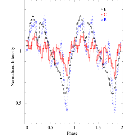
Figure 4: XIS pulse profiles folded with the same period and period derivative for the same epoch as Fig. 3 for segments B, C and E are overlaid. The pulse fraction change in C, and the shift in phase is apparent compared to B and E.

Figure 5: The left- and right- hand panels show the energy resolved pulse profiles for segment E for XIS and PIN respectively folded with a period of 36.930 s and a period derivative of $3.1847\times{10^{-8}}$ s s^-1 at epoch MJD 55830. The pulse profiles do not show dependence on energy.

3 Spectral Analysis

We performed time averaged spectral analysis of OAO 1657–415 using spectra from all the three XISs and the PIN. Spectral fitting was performed using XSPEC v12.7.1. Artificial structures are known in the XIS spectra around the Si edge and Au edge and the energy range of 1.75-2.23 keV is usually not used for spectral fitting. Additionally, owing to strong absorption, the spectrum of OAO 1657–415 has very limited statistics below 3 keV. For spectral fit we have therefore, chosen the energy range of 3-10 keV for the XISs and 15-70 keV for the PIN spectrum respectively. We fitted the spectra simultaneously with all parameters tied, except the relative instrument normalizations which were kept free. The 2048 channel XIS spectra were rebinned by a factor of 10 up to 5 keV, by 2 from 5 to 7 keV and by 14 for the rest. The PIN spectra were binned by a factor of 4 till 22 keV, by 6 from 22 to 45 keV, and by 10 for the rest. To fit the continuum for the spectra, we tried using the standard continuum models used for HMXBs like HIGHECUT (White, Swank & Holt, 1983; Heindl et al., 2001), NPEX (Mihara, 1995), COMPTT (Titarchuk, 1994) and FDCUT (Tanaka, 1986). Good fit for the average spectra was obtained with two of the continuum models, NPEX and HIGHECUT. In the NPEX model, the photon index of the second power-law component was fixed at 2.0. For both, a partial covering absorption and two Gaussian emission line components were required to account for the two lines at 6.4 keV and 7.1 keV, which correspond to $K{\alpha}$ and $K{\beta}$ fluorescence emission lines of iron. For the time-averaged spectra showed some dip like residuals in the PIN data. We used cyclotron absorption profiles GABS and CYCLABS to account for the residuals, of which CYCLABS provided a better fit. However, all parameters of the cyclotron line could not be constrained and we have fixed the width of the line to 2 keV. Inclusion of CYCLABS along with NPEX resulted in a decrease in $\chi^{2}$ from 628 (415 degrees of freedom) to 618 (413 degrees of freedom). The dip like feature for HIGHECUT and NPEX were seen at 34 and 32 keV, respectively. We note here that possible presence of a cyclotron line in OAO 1657–415 at a similar energy was reported earlier from Beppo-SAX observations (Orlandini et al., 1999).
Fig. 6 shows the average spectra fitted with NPEX model and the spectral parameters for the best fit obtained for the two models are given in Table 2.
To calculate the significance of emission line features which are additive components in XSPEC like the iron line emission, the F-test routine in XSPEC package is best suited to perform the significance test barring precautions as mentioned in Protassov et al. (2002). However, for the purpose of detecting the significance of multiplicative components like the cyclotron line, the same is not valid. Hence, we use the F-test routine available in IDL package MPFTEST for significance test of cyclotron line (DeCesar et al., 2013). The probability of chance improvement (PCI) is evaluated for the NPEX model used to fit the spectrum with and without cyclotron line. The estimated PCI values after addition of cyclotron line component to the NPEX is $\sim$ 45 % . Therefore, a cyclotron line at around 36 keV which was detected with Beppo-SAX is not confirmed in the Suzaku spectrum.

Figure 6: Time-averaged spectrum for OAO 1657–415 using the NPEX model. The middle panel shows the residue without using CYCLABS and the lowermost panel shows the residue when CYCLABS is included.

3.1 Time-resolved Spectroscopy

The variable hardness ratio shown in Fig. 1 indicates significant spectral changes during the duration of the observation. To probe into the details of the spectral variations, we divided the light curve into five segments on the basis of their hardness ratio as shown in Fig. 1. The time-resolved spectrum was fitted with the same model as used for time-averaged spectra. However, a partial covering absorption was not required for the segments A, B and D. Also, the negative residuals around 33 keV in the PIN data mentioned in the previous section and shown in Fig. 7 was visible only in the two segments A and C. The variations of the spectral parameters with time obtained from spectral fits with the two continuum models NPEX and HIGHECUT are shown in Fig. 8. Variations of the spectral parameters obtained with the two models are consistent indicating the robustness of the results. As seen in Fig. 8, the equivalent widths for the two iron line elements increase largely in the third segment C. Segments A and C have similar hardness ratios. However, the equivalent widths and $N_{\rm H}$ in segment A is smaller compared to segment C. This difference led us to check the variation of equivalent widths and $N_{\rm H}$ with time in finer time intervals. This variation is shown in Fig. 9. We shall discuss about this further in the next section.

Table 2: Best-fitting parameters of the time–averaged spectra for OAO 1657–415 during the Suzaku observation. Errors quoted are for 90 per cent confidence range.

Parameter	NPEX	HIGHECUT
$N_{\rm H1}$ ($10^{22}$ atoms cm-2)	$15.6_{-0.9}^{+0.8}$	$16.7_{-0.65}^{+0.71}$
$N_{\rm H2}$ ($10^{22}$ atoms cm-2)	$34_{-3.1}^{+3.5}$	$42.7_{-5.8}^{+9.1}$
PowIndex	$0.22$*${}_{-0.01}^{+0.02}$	$0.52_{-0.02}^{+0.01}$
CvrFract	$0.58_{-0.04}^{+0.05}$	$0.46_{-0.03}^{+0.03}$
Ehighecut (keV)	$8.6_{-0.14}^{+0.26}$	–
Ecut (keV)	–	$6.2_{-0.17}^{+0.16}$
Efold (keV)	–	$16.6_{-0.6}^{+0.4}$
Depth(keV)	$0.11_{-0.05}^{+0.05}$	$0.1_{-0.04}^{0.04}$
Cyclabs(keV)	$32_{-2.0}^{+2.3}$	$34_{-2.4}^{+5.6}$
K$\alpha$ line (keV)	$6.44_{-0.003}^{+0.001}$	$6.43_{-0.002}^{+0.003}$
K$\beta$ line (keV)	$7.09_{-0.01}^{+0.01}$	$7.11_{-0.006}^{+0.007}$
Equivalent Width for K$\alpha$ line (keV)	$0.261_{-0.006}^{+0.005}$	$0.261_{0.005}^{+0.006}$
Equivalent Width for K$\beta$ line (keV)	$0.081_{-0.004}^{+0.004}$	$0.074_{-0.003}^{+0.005}$
$\chi^{2}_{\nu}$/d.o.f	1.49/413 (1.51/415 without CYCLABS)	1.46/417 (1.47/419 without CYCLABS)

$*$ Photon-index of the second power-law component of the NPEX model is frozen to 2.0, as mentioned in the text.

$\begin{array}[]{cc}\includegraphics[height=202.35622pt,width=144.54pt,angle={-90}]{B.ps}&\includegraphics[height=202.35622pt,width=173.44756pt,angle={-90}]{A_npex_tot1.ps}\\ \includegraphics[height=202.35622pt,width=130.08621pt,angle={-90}]{D.ps}&\includegraphics[height=202.35622pt,width=173.44756pt,angle={-90}]{C_npex_tot1.ps}\\ \includegraphics[height=202.35622pt,width=130.08621pt,angle={-90}]{E.ps}\end{array}$

Figure 7: Time-resolved spectrum for OAO 1657–415 using the NPEX model. The middle panel for segments A and C shows the residue obtained after fitting without using CYCLABS and the lowermost panel in both represent the residuals after CYCLABS is fitted.

Figure 8: Variation of spectral parameters with time using NPEX is shown in the left and to the right is the variation of spectral parameters using HIGHECUT model. The topmost panel in both figures show count rate.

Figure 9: Variation of equivalent width for Gaussian line elements at 6.5 and 7.1 keV for the NPEX model to the left and HIGHECUT to the right.

Figure 10: Histogram of the orbit averaged count rate of OAO 1657–415 for Swift-BAT and MAXI-GSC. The count rate (X-axis) is normalized to that of Crab nebula for the respective instrument. The arrows represent the orbit corresponding to Suzaku observation.

4 Discussion

4.1 Flux and spectral variability

The variation in intensity for this source over a large number of orbits taken together has been studied in the past (Barnstedt et al., 2008). Fig. 10 shows the intensity (normalized to Crab) histograms with MAXI-GSC (MJD 55063–56661) and Swift-BAT (MJD 53415–56617). The orbit averaged intensity corresponding to this Suzaku observation are marked with arrows in the two panel of Fig. 10 which indicates that in this orbit OAO 1657–415 did not have extreme property i.e. very high or very low count rate compared to the long-term average. In this paper, we discuss the variability of OAO 1657–415 in time-scales that is a fraction of the orbital period.
Segment C makes an interesting study. As depicted in Fig. 4, we see that pulse fraction suddenly goes very low in C compared to the other segments. During this segment, the equivalent width for both Gaussian line elements at 6.4 and 7.1 keV increases compared to other segments. This change of pulse fraction in C is more apparent for XIS data than PIN data. This can be due to the dominance of the Fe line photons, which are unpulsed in nature. The variation in the characteristics of the segments are summarized below:

1. Segment A: large hardness ratio with large $N_{\rm H}$ and moderate equivalent width.

2. Segment B: hardness ratio is low with low $N_{\rm H}$ and low equivalent width.

3. Segment C: hardness ratio is high with very large $N_{\rm H}$ and large equivalent width.

4. Segment D: same as B.

5. Segment E: same as B, but flux higher by a factor of $\sim$ 6.

One possible explanation for the above observations could be as follows: during segment A, the pulsar may be passing behind a dense clump of matter. This causes absorption of soft X-rays, leading to an increase in hardness ratio and large value of $N_{\rm H}$ but low equivalent width if the clump subtends a small solid angle to the source. If the neutron star had been passing through the clump, a large equivalent width would be seen.
During segment B, the hardness ratio, $N_{\rm H}$ and equivalent width are low. Here the pulsar may be passing through a region where there is very scanty material.
In segment C however, a large increase in hardness ratio, $N_{\rm H}$, and equivalent width indicates that instead of being behind a cloud, the neutron star is now passing through a dense clump of matter. The large soft X-ray absorption leads to increase in the measured hardness ratio and $N_{\rm H}$, while a 4$\pi$ solid angle of the clump causes a large equivalent width of the iron fluorescence lines. This should also lead to an increase in the mass accretion rate on to the neutron star and its X-ray luminosity, probably with a delay corresponding to the viscous time-scale from the material capture radius in the accretion disc to the neutron star.
In segment D, the hardness ratio, $N_{\rm H}$ and equivalent width are all low (same scenario as segment B).
In segment E also, the hardness ratio, $N_{\rm H}$ and equivalent width are low. However, there is an increase in luminosity (starting from segment D that lasts through segment E). This could be the increase in luminosity resulting from the increased mass capture from the clump that the neutron star encountered in segment C. The time lag between the increase mass accretion in segment C, and the increase in X-ray luminosity which is manifested in segments D and E is less than one day.
The viscous time-scale depends on the specific angular momentum of the captured material with respect to the neutron star. In the case of the HMXB GX 301-2, which has an orbital period of 41.5 d and which shows a large flare every orbit at the orbital phase of 0.95, an enhanced accretion at orbital phase 0.92($\sim$ 1.2 d earlier than the flare) was shown to reproduce the flare (Pravdo & Ghosh, 2001).

4.2 Comparison with SFXTs and supergiant systems

The spectral and intensity variations of the Suzaku observation in this source shows that the stellar wind emitted from the companion star is inhomogeneous with many clumps as indicated in Oskinova, Feldmeier & Kretschmar (2013). A rough estimate about the size of the clump which the neutron star passes through during segment C is made as follows:
The time of passage of the neutron star through the segment C is $\sim$ 47 ks. Assuming the relative velocity of the wind $v_{\mathrm{rel}}=300\ \mathrm{km\ s^{-1}}$ at the neutron star, we obtain the clump radius of segment C, $R_{c}\simeq v_{\mathrm{rel}}t_{f}/2$ = $7\times 10^{11}$ cm. For the C segment, the column density of $N_{\rm H}$ is $\sim$ 10²⁴ cm^-2.
Hence, the mass of clump is $\sim 3\times 10^{24}\rm{g}$ .
In similar lines, Bozzo et al. (2011) discussed that X-ray flares observed from an SFXT, IGR J18410–0535 as being due to accretion of matter from a massive clump on to the neutron star, the mass of the clump being $\sim 1.4\times 10^{22}\rm{g}$.
Here, it is worthwhile to note the similarity of OAO 1657–415 with Vela X-1. Vela X-1 is embedded in the dense stellar wind of its optical companion (Nagase et al., 1986) and displays a strong time variability Kreykenbohm et al. (2008); Soffitta et al. (2008). Owing to the high X-ray variability of both OAO 1657–415 and Vela X-1, they can be seen as a class of systems which could represent a possible link between SFXTs and normal HMXBs.
SFXTs show irregular outbursts, lasting from minutes to hours, with peak X-ray luminosities between $10^{36}$ and $10^{37}ergs^{-1}$ in contrast to a quiescent phase when the typical luminosities maybe $10^{32}ergs^{-1}$ (González-Riestra et al., 2004; Sidoli et al., 2005; Grebenev & Sunyaev, 2005; Lutovinov et al., 2005; Masetti et al., 2006; Götz et al., 2007). These variations could be due to the clumpiness of stellar wind which may lead to variations of the density and velocity of matter around the neutron star, resulting in the fluctuation of the accretion rate Kreykenbohm et al. (2008); Ducci et al. (2009) or when accretion is regulated by magnetospheric barrier (Bozzo, Falanga & Stella, 2008). Though the study of variability of OAO 1657–415 here is in longer time-scales compared to SFXTs, further study of this class of objects will help us in better understanding of the physical origin of the X-ray variability and provide a link between SFXTs and supergiant HMXBs.

5 Acknowledgements

The data for this work have been obtained through the High Energy Astrophysics Science Archive (HEASARC) Online Service provided by NASA/GSFC. We have also made use of public light curves from Swift and MAXI site. We would also like to thank the anonymous referee and Sachindra Naik for invaluable comments and suggestions.

References

- Audley et al. (2006) Audley M. D., Nagase F., Mitsuda K., Angelini L., Kelley R. L., 2006, MNRAS, 367, 1147
- Barnstedt et al. (2008) Barnstedt J. et al., 2008, A&A, 486, 293
- Baykal (1997) Baykal A., 1997, A&A, 319, 515
- Baykal (2000) Baykal A., 2000, MNRAS, 313, 637
- Bildsten et al. (1997) Bildsten L. et al., 1997, ApJS, 113, 367
- Bozzo, Falanga & Stella (2008) Bozzo E., Falanga M., Stella L., 2008, ApJ, 683, 1031
- Bozzo et al. (2011) Bozzo E. et al., 2011, A&A, 531, A130
- Chakrabarty et al. (1993) Chakrabarty D. et al., 1993, ApJ, 403, L33
- Chakrabarty et al. (2002) Chakrabarty D., Wang Z., Juett A. M., Lee J. C., Roche P., 2002, ApJ, 573, 789
- Corbet (1986) Corbet R. H. D., 1986, MNRAS, 220, 1047
- DeCesar et al. (2013) DeCesar M. E., Boyd P. T., Pottschmidt K., Wilms J., Suchy S., Miller M. C., 2013, ApJ, 762, 61
- Ducci et al. (2009) Ducci L., Sidoli L., Mereghetti S., Paizis A., Romano P., 2009, MNRAS, 398, 2152
- Fukazawa et al. (2009) Fukazawa Y. et al., 2009, PASJ, 61, 17
- González-Riestra et al. (2004) González-Riestra R., Oosterbroek T., Kuulkers E., Orr A., Parmar A. N., 2004, A&A, 420, 589
- Götz et al. (2007) Götz D., Falanga M., Senziani F., De Luca A., Schanne S., von Kienlin A., 2007, ApJ, 655, L101
- Grebenev & Sunyaev (2005) Grebenev S. A., Sunyaev R. A., 2005, Astronomy Letters, 31, 672
- Heindl et al. (2001) Heindl W. A., Coburn W., Gruber D. E., Rothschild R. E., Kreykenbohm I., Wilms J., Staubert R., 2001, ApJ, 563, L35
- Jenke et al. (2012) Jenke P. A., Finger M. H., Wilson-Hodge C. A., Camero-Arranz A., 2012, ApJ, 759, 124
- Koyama et al. (2007) Koyama K. et al., 2007, PASJ, 59, 23
- Kreykenbohm et al. (2008) Kreykenbohm I. et al., 2008, A&A, 492, 511
- Lutovinov et al. (2005) Lutovinov A., Revnivtsev M., Gilfanov M., Shtykovskiy P., Molkov S., Sunyaev R., 2005, A&A, 444, 821
- Masetti et al. (2006) Masetti N. et al., 2006, A&A, 449, 1139
- Mason et al. (2009) Mason A. B., Clark J. S., Norton A. J., Negueruela I., Roche P., 2009, A&A, 505, 281
- Mihara (1995) Mihara T., 1995, PhD thesis, , Dept. of Physics, Univ. of Tokyo (M95), (1995)
- Mitsuda et al. (2007) Mitsuda K. et al., 2007, PASJ, 59, 1
- Nagase et al. (1986) Nagase F., Hayakawa S., Sato N., Masai K., Inoue H., 1986, PASJ, 38, 547
- Orlandini et al. (1999) Orlandini M., dal Fiume D., del Sordo S., Frontera F., Parmar A. N., Santangelo A., Segreto A., 1999, A&A, 349, L9
- Oskinova, Feldmeier & Kretschmar (2013) Oskinova L. M., Feldmeier A., Kretschmar P., 2013, in IAU Symposium, Vol. 290, IAU Symposium, Zhang C. M., Belloni T., Méndez M., Zhang S. N., eds., pp. 287–288
- Polidan et al. (1978) Polidan R. S., Pollard G. S. G., Sanford P. W., Locke M. C., 1978, Nature, 275, 296
- Pravdo & Ghosh (2001) Pravdo S. H., Ghosh P., 2001, ApJ, 554, 383
- Protassov et al. (2002) Protassov R., van Dyk D. A., Connors A., Kashyap V. L., Siemiginowska A., 2002, ApJ, 571, 545
- Sidoli et al. (2005) Sidoli L., Vercellone S., Mereghetti S., Tavani M., 2005, A&A, 429, L47
- Soffitta et al. (2008) Soffitta P. et al., 2008, The Astronomer’s Telegram, 1782, 1
- Takahashi et al. (2007) Takahashi T. et al., 2007, PASJ, 59, 35
- Tanaka (1986) Tanaka Y., 1986, in Lecture Notes in Physics, Berlin Springer Verlag, Vol. 255, IAU Colloq. 89: Radiation Hydrodynamics in Stars and Compact Objects, Mihalas D., Winkler K.-H. A., eds., p. 198
- Titarchuk (1994) Titarchuk L., 1994, ApJ, 434, 570
- White & Pravdo (1979) White N. E., Pravdo S. H., 1979, ApJ, 233, L121
- White, Swank & Holt (1983) White N. E., Swank J. H., Holt S. S., 1983, ApJ, 270, 711