Where geography lives?
A projection approach for spatial confounding

Abstract

Spatial confounding between the spatial random effects and fixed effects covariates has been recently discovered and showed that it may bring misleading interpretation to the model results. Solutions to alleviate this problem are based on decomposing the spatial random effect and fitting a restricted spatial regression. In this paper, we propose a different approach: a transformation of the geographic space to ensure that the unobserved spatial random effect added to the regression is orthogonal to the fixed effects covariates. Our approach, named SPOCK, has the additional benefit of providing a fast and simple computational method to estimate the parameters. Furthermore, it does not constrain the distribution class assumed for the spatial error term. A simulation study and a real data analysis are presented to better understand the advantages of the new method in comparison with the existing ones.

1 Introduction

Spatial generalized linear mixed models (SGLMM) for areal data analysis have become a common tool for data analysis in recent years with the availability of spatially referenced data sets. Besag et al. (1991) introduced a hierarchical modeling adding random spatial effects to a generalized linear regression model. The spatial dependence is captured by a latent Gaussian Markov Random Field (GMRF). One important advantage of this GMRF approach is to induce a sparse precision matrix that allows for intuitive conditional interpretation and fast Bayesian computation (Rue and Held, 2005). In the past 20 years, Besag et al. (1991) model (hereafter ICAR) has become the most popular areal model for its flexibility and due to its implementation in the WinBUGS software (Lunn et al., 2000), which is freely available.

Most spatial data are observational rather than experimental and we commonly observe correlation or multicollinearity between the covariates, also called explanatory or fixed-effect variables. As a consequence of this multicollinearity, in non-spatial regression problems, the estimated coefficients are affected by the presence of the other covariates (Mosteller and Tukey, 1997). This is called confounding and it can lead to implausible estimates. It also affects the variance of the covariates’ coefficients estimators which are inflated with respect to what one would have in case the covariates were orthogonal to each other.

In the spatial context, Clayton et al. (1993) and Reich et al. (2006) identified the existence of confounding between the fixed and random effects in SGLMM. In their work, Reich et al. (2006) show that explanatory variables having a spatial pattern may confound with the spatial random effects, resulting in fixed effects estimates that are counterintuitive. Thus, they propose an alternative model, called hereafter RHZ model, to alleviate this confounding problem. The RHZ model projects the spatial effects into the orthogonal space spanned by the explanatory variables.

Another well known shortcoming of SGLMM is the computational burden when dealing with high dimensional latent effects. Recently, Hughes and Haran (2013) introduce an alternative model (hereafter, HH model) that alleviates spatial confounding and, at the same time, requires less computational effort. They also consider an orthogonal projection of the spatial effects in a way that takes into account the explanatory variables and the spatial structure. Properties of the HH model was further studied by Murakami and Griffith (2015).

The main idea behind the Reich et al. (2006) and Hughes and Haran (2013) methods is to project the unobserved spatial effects vector in the linear space orthogonal to the explanatory variables. As a consequence, they end up with a precision matrix that is far from sparse losing one of the main advantages of the Markov random fields. Another drawback from RHZ and HH methods is that they only work with spatial effects restricted to follow the ICAR model. Therefore,they do not allow for more flexible spatial structures such as the proper CAR model (Besag, 1974; Leroux et al., 1999; Rodrigues and Assunção, 2012).

From a geostatistical perspective, Paciorek (2010) dealt with the effects of confounding between the spatial random effects and possible explanatory variables. He showed that it can lead to bias in the parameter estimation. Hanks et al. (2015) also studied the effects of spatial confounding in the continuous support situation. They proposed a posterior predictive approach to correct a bias on the credibility intervals produced by RHZ.

In this paper, we adopt a different approach to deal with spatial confounding in lattice data. Rather than removing the explanatory variables effect from the spatial random effects, we alter the spatial pattern of the map by purging the covariates from the geography. We do this by projecting the spatial coordinates of the areas into the orthogonal space of the covariates and hence producing a new set of geographical coordinates. These new coordinates induce a different neighborhood structure for the areas that are used to define a different precision matrix. The transformed geography retains the spatial neighborhood that is orthogonal to the covariates. One important consequence of our approach is that we maintain the sparsity of the spatial effects precision matrix allowing for very fast Bayesian computation while controlling for spatial confounding.

Our new approach is called SPOCK, an acronym for SPatial Orthogonal Centroid “K”orrection. SPOCK led us to understand better the role of spatial confounding and its effect on parameter estimation. It gives a more clear understanding of the conceptual differences between the parameters in models that do and do not alleviate spatial confounding. In a striking example, Reich et al. (2006) showed that spatial confounding may provide counter intuitive results in some situations. Sign and relevance of covariates can change drastically after one adds a spatial random effect in a lattice-data regression model. Some important questions arise. When does that occur? Is it always necessary to correct for spatial confounding? If not, when to do so? There is an on-going discussion among the researchers about the need for spatial confounding correction and the meaning of the resulting fixed-effect parameters (Paciorek, 2010; Hanks et al., 2015). With our model as a framework, in the simulation study of Section 5, we revisit these questions and try to better understand what are the consequences of correcting for spatial confounding and when it is adequate to do so.

The contributions of this paper are the following:

• a new conceptual approach, SPOCK, to handle spatial confounding;

• because our approach retains the Markovian property, it is extremely efficient for Bayesian computation even in high dimension problems generated by maps with very large number of areas;

• in contrast with the present alternatives, SPOCK has no restriction to the type of spatial structure for the random effects;

• SPOCK is very simple to implement and it can be run in any Bayesian spatial software such as WinBUGS and R-INLA (Rue et al., 2009).

The paper proceeds as follows. In Section 2 we review the traditional SGLMM model and present a summary of the RHZ and HH methods. Section 3 introduces SPOCK and its properties are discussed. In Section 5, a simulation study is performed to compare the proposed method against RHZ and HH methods in terms of precision of estimates and time. It also provides insights on when to correct for spatial confounding and what are the consequences of it. In Section 6, we revisit the Slovenia data (Zadnik and Reich, 2006) to illustrate the conclusion obtained with the three models and their computational efficiency. Finally, the paper concludes with a discussion in Section 7.

2 Existing Methods

2.1 SGLMM

Spatial Generalized Linear Mixed Models (SGLMM) is a wide class of models that accommodates spatial dependence through a random effect term. Let $Y_{i}$ be the observation of an area $i$, $i=1,\ldots,n$ with distribution given by

$$Y_{i}\sim\pi(y|\mu_{i},{\boldsymbol{\delta}},{\boldsymbol{X}}_{i},\beta)$$

$$g(\mu_{i})={\boldsymbol{X}}_{i}{\boldsymbol{\beta}}+\theta_{i},$$

where ${\boldsymbol{\beta}}$ is the fixed effects coefficients vector and ${\boldsymbol{X}}$ is a $n\times q$ full-rank design matrix with the covariates. Typically, ${\boldsymbol{X}}$ includes a first column of constant values equal to 1. We let ${\boldsymbol{X}}_{i}$ be its $i$-th row, $g$ is an appropriate link function, and $\mu_{i}=E(Y_{i}|{\boldsymbol{X}}_{i})$. The vector of hyperparameters of the distribution is ${\boldsymbol{\delta}}$. Finally, ${\boldsymbol{\theta}}$ represents a vector with spatially structured random variables capturing the spatial patterns shared by the areas in study.

The most simple instance of this model is the Gaussian model where

$$Y_{i}|\mu_{i},\tau_{\epsilon} \sim N(\mu_{i},\tau_{\epsilon})$$

$$\mu_{i} = {\boldsymbol{X}}_{i}{\boldsymbol{\beta}}+\theta_{i}.$$ (1)

Traditionally the spatial random effect ${\boldsymbol{\theta}}^{\top}=(\theta_{1},\ldots,\theta_{n})$ is defined as an intrinsic conditional autoregressive (ICAR) models introduced by Besag et al. (1991). The prior specification of the ICAR model is given by

$$\pi({\boldsymbol{\theta}}|\tau_{\theta})\propto\tau_{\theta}^{r({\boldsymbol{Q}})/2}\exp{\left(-\frac{\tau_{\theta}}{2}{\boldsymbol{\theta}}^{\top}{\boldsymbol{Q}}{\boldsymbol{\theta}}\right)}$$ (2)

where ${\boldsymbol{Q}}$ is the precision matrix, $r({\boldsymbol{Q}})$ is the rank of the ${\boldsymbol{Q}}$ matrix (Lavine and Hodges, 2012) and $\tau_{\theta}$ is the spatial precision. The matrix ${\boldsymbol{Q}}$ is associated with the geographical structure represented by a neighborhood graph $\mathcal{G}$. In this graph, each area is a node located on its spatial centroid and neighboring areas are connected by edges. A pair of areas $(i,j)$ that are not neighbors has ${\boldsymbol{Q}}_{ij}={\boldsymbol{Q}}_{ji}=0$. Rue and Held (2005) showed that the non-zero pattern in ${\boldsymbol{Q}}$ defines the conditional dependence structure of the graph under study. In other words, with the underlying geographical neighborhood in analysis, it is possible to define the non-zero pattern of ${\boldsymbol{Q}}$. Moreover, the precision matrix ${\boldsymbol{Q}}$ is commonly sparse and this can be computationally explored to substantially improve speed in model fitting.

2.2 Non-Confounding SGLMM

Clayton et al. (1993) introduced the concept of spatial confounding between the fixed effects estimates and the spatial random effects in SGLMM. However, only recently, Reich et al. (2006) revisited the problem motivated by a striking case study where the credibility interval for a certain fixed effect coefficient changes drastically after introducing the spatial random effects. They proposed an alternative method to alleviate this confounding problem. In general, the idea proposed is to include in the model a random effect that belong to the orthogonal space of the fixed effects predictors. A new $\mathbb{R}^{n}$ basis can be used to re-express

$${\boldsymbol{\theta}}={\boldsymbol{\theta}}^{X}+{\boldsymbol{\theta}}^{\perp}={\boldsymbol{K}}{\boldsymbol{\theta}}_{1}+{\boldsymbol{L}}{\boldsymbol{\theta}}_{2}$$ (3)

where ${\boldsymbol{K}}$ is a $n\times q$ matrix that has the same span as ${\boldsymbol{X}}$, ${\boldsymbol{L}}$ is a $n\times(n-q)$ matrix whose columns lies in the orthogonal space of ${\boldsymbol{X}}$, and ${\boldsymbol{\theta}}_{1}$ and ${\boldsymbol{\theta}}_{2}$ are vectors with dimensions $q$ and $n-q$, respectively. Equation (1) can be represented as

$$Y_{i}|\mu_{i},\tau_{\epsilon} \sim N(\mu_{i},\tau_{\epsilon})$$

$$\mu_{i} = {\boldsymbol{X}}_{i}{\boldsymbol{\beta}}+{\boldsymbol{K}}_{i}\theta_{i1}+{\boldsymbol{L}}_{i}\theta_{i2},$$

where ${\boldsymbol{K}}_{i}$ and ${\boldsymbol{L}}_{i}$ are the $i$-th rows of ${\boldsymbol{K}}$ and ${\boldsymbol{L}}$, respectively. The vector ${\boldsymbol{\theta}}$ follows the ICAR distribution in (2). Using this parametrization, it was shown that ${\boldsymbol{K}}$ causes a confounding in the estimates of ${\boldsymbol{\beta}}$. Reich et al. (2006) suggested the removal of the ${\boldsymbol{K}}$ component leading to the RHZ model:

$$Y_{i}|\mu_{i},\tau_{\epsilon} \sim N(\mu_{i},\tau_{\epsilon})$$

$$\mu_{i} = {\boldsymbol{X}}_{i}{\boldsymbol{\beta}}+{\boldsymbol{L}}_{i}\theta_{i2}$$

$${\boldsymbol{\theta}}_{2} \sim N_{n-q}\left(0,{\boldsymbol{L}}^{\top}{\boldsymbol{Q}}{\boldsymbol{L}}\right).$$ (4)

Although it solves the confounding between the spatial random effects and the estimates of the fixed effects, Hughes and Haran (2013) noticed that this correction is computationally inefficient. The reason is that the new precision matrix generated by Eq (4) is not sparse and has dimension $n-q\approx n$. To reduce the computational demand of the RHZ model they proposed a sparse alternative model. This new model uses the so-called Moran operator ${\boldsymbol{P}}^{\bot}{\boldsymbol{A}}{\boldsymbol{P}}^{\bot}$ where ${\boldsymbol{A}}$ is the graph zero/one adjacency matrix and

$${\boldsymbol{P}}^{\bot}={\boldsymbol{I}}-{\boldsymbol{X}}({\boldsymbol{X}}^{\top}{\boldsymbol{X}})^{-1}{\boldsymbol{X}}^{\top}$$ (5)

is the projection matrix into the orthogonal space of the span of ${\boldsymbol{X}}$. They showed that the Moran operator retains the spatial patterns of the data and it is only necessary to select the $h\ll n$ higher eigenvalues of the spectrum of the Moran operator. In this way, they were able to reduce the dimension of the random effect maintaining the spatial information necessary in model estimation. The HH model is defined as:

$$Y_{i}|\mu_{i},\tau_{\epsilon} \sim N(\mu_{i},\tau_{\epsilon}{\boldsymbol{I}})$$

$$\mu_{i} = {\boldsymbol{X}}_{i}{\boldsymbol{\beta}}+{\boldsymbol{M}}_{i}\theta_{i2}$$

$${\boldsymbol{\theta}}_{2} \sim N_{h}\left(0,{\boldsymbol{M}}^{\top}{\boldsymbol{Q}}{\boldsymbol{M}}\right),$$

where ${\boldsymbol{M}}$ contains the first $h$ eingenvectors of the Moran operator.

3 Purging the covariates from the geography

Although Reich et al. (2006) and Hughes and Haran (2013) were successful in alleviating the confounding and in reducing the dimension of the spatial random effects as presented in Section 2.2, their approaches have two main drawbacks: 1) the RHZ and HH models do not accept parameters in the precision matrix ${\boldsymbol{Q}}$ (e.g., Besag, 1974; Leroux et al., 1999; Rodrigues and Assunção, 2012); 2) both lost the original SGLMM model sparsity of the precision matrix and hence do not take advantage of the Markov property in the Bayesian calculations. In order to propose a fast SGLMM that alleviates the confounding problem, we introduce SPOCK, a novel approach to the problem capable of maintaining the Markov properties of the precision matrix as well as allowing for unknown parameters in the matrix ${\boldsymbol{Q}}$. SPOCK not only produces a fast alternative to RHZ and HH but, more importantly, it also represents a new and rather different conceptual perspective on how to deal with the problem. We will show that this new way of seeing the spatial confounding can help in clarifying the discussion about the need for and the consequences of the confounding alleviation.

Instead of reparametrizing the random effects vector by decomposing it into two orthogonal subspaces, we project the neighborhood graph vertices into the orthogonal space of the covariate matrix ${\boldsymbol{X}}$. We transform the geographical centroids inducing a new neighborhood structure that is not influenced by the covariates. Spatial effects defined on this transformed geography will not be correlated with the predictors. The projected image of the original graph (hereafter, projected graph) allows us to keep the sparsity of the precision matrix ${\boldsymbol{Q}}$ and the Markov properties of random effects, making the estimation of our model more efficient than RHZ and HH (Rue and Held, 2005). Since SPOCK works only by redefining the non-zero pattern of ${\boldsymbol{Q}}$ by means of the projected graph, it allows the user to adjust a variety of parameter-based spatial structure such as Besag (1974); Besag et al. (1991); Leroux et al. (1999); Rodrigues and Assunção (2012).

Let ${\boldsymbol{s}}=[{\boldsymbol{s}}_{1},{\boldsymbol{s}}_{2}]$ be the $n\times 2$ matrix with the areas’ centroids coordinates. Assume that $\psi(s_{1},s_{2})$ is a Gaussian random field conceptually defined for any location $(s_{1},s_{2})$ in the map and that ${\boldsymbol{\theta}}=(\psi_{1},\ldots,\psi_{n})$ where $\psi_{i}=\psi(s_{i1},s_{i2})$. Let $(s_{10},s_{20})$ be a reference location such as a central position in the map. Let $\frac{\partial\psi}{\partial s_{1}}$ and $\frac{\partial\psi}{\partial s_{2}}$ be the partial derivatives evaluated at $(s_{10},s_{20})$. When the field is smooth enough, the value $\psi(s_{1},s_{2})$ in an arbitrary location $(s_{1},s_{2})$ can be written as

$$\psi(s_{1},s_{2}) = \psi(s_{10},s_{20})+\left(s_{1}-s_{10},s_{2}-s_{20}\right)\left[\begin{array}[]{c}\frac{\partial\psi}{\partial s_{1}}\\ \frac{\partial\psi}{\partial s_{2}}\end{array}\right]+R(s_{1},s_{2},s_{10},s_{20})$$ (8)

$$= \gamma_{0}+\gamma_{1}(s_{1}-s_{10})+\gamma_{2}(s_{2}-s_{20})+R(s_{1},s_{2},s_{10},s_{20})\>.$$ (9)

Evaluating the expression (9) at the centroids ${\boldsymbol{s}}$ and organizing the result as a vector, we have

$${\boldsymbol{\theta}}=\psi({\boldsymbol{s}}) = \gamma_{0}{\boldsymbol{1}}+\gamma_{1}({\boldsymbol{s}}_{1}-s_{10}{\boldsymbol{1}})+\gamma_{2}({\boldsymbol{s}}_{2}-s_{20}{\boldsymbol{1}})+{\boldsymbol{R}}({\boldsymbol{s}}_{1},{\boldsymbol{s}}_{2},s_{10},s_{20})$$

$$= (\gamma_{0}-s_{10}-s_{20}){\boldsymbol{1}}+\gamma_{1}{\boldsymbol{s}}_{1}+\gamma_{2}{\boldsymbol{s}}_{2}+{\boldsymbol{R}}({\boldsymbol{s}}_{1},{\boldsymbol{s}}_{2},s_{10},s_{20})$$

$$= [{\boldsymbol{1}},{\boldsymbol{s}}_{1},{\boldsymbol{s}}_{2}]{\boldsymbol{\gamma}}+{\boldsymbol{R}}\>.$$

In this way, we expressed the spatial random effects with a linear component on the coordinates ${\boldsymbol{s}}$. Returning to the SGLMM model, we can rewrite (1) as

$${\boldsymbol{Y}} = {\boldsymbol{X}}{\boldsymbol{\beta}}+[{\boldsymbol{1}},{\boldsymbol{s}}_{1},{\boldsymbol{s}}_{2}]{\boldsymbol{\gamma}}+{\boldsymbol{R}}$$ (10)

$$= {\boldsymbol{X}}{\boldsymbol{\beta}}+{\boldsymbol{P}}[{\boldsymbol{1}},{\boldsymbol{s}}_{1},{\boldsymbol{s}}_{2}]{\boldsymbol{\gamma}}+{\boldsymbol{P}}^{\bot}[{\boldsymbol{1}},{\boldsymbol{s}}_{1},{\boldsymbol{s}}_{2}]{\boldsymbol{\gamma}}+{\boldsymbol{R}}$$

$$= {\boldsymbol{X}}\left({\boldsymbol{\beta}}+\left({\boldsymbol{X}}^{\top}{\boldsymbol{X}}\right)^{-1}{\boldsymbol{X}}^{\top}[{\boldsymbol{1}},{\boldsymbol{s}}_{1},{\boldsymbol{s}}_{2}]{\boldsymbol{\gamma}}\right)+{\boldsymbol{P}}^{\bot}[{\boldsymbol{1}},{\boldsymbol{s}}_{1},{\boldsymbol{s}}_{2}]{\boldsymbol{\gamma}}+{\boldsymbol{R}}$$

$$= {\boldsymbol{X}}{\boldsymbol{\beta}}^{*}+{\boldsymbol{P}}^{\bot}[{\boldsymbol{1}},{\boldsymbol{s}}_{1},{\boldsymbol{s}}_{2}]{\boldsymbol{\gamma}}+{\boldsymbol{R}}\>,$$

where we used that ${\boldsymbol{I}}={\boldsymbol{P}}+{\boldsymbol{P}}^{\bot}$ with ${\boldsymbol{P}}^{\bot}$ defined in (5). One of the main advantages of expression (10) is to clearly and intuitively answer to Hodges and Reich (2011) when they ask how “adding spatially correlated errors can mess up the fixed effect you love”. The ${\boldsymbol{X}}$ fixed effect is messed up by the spatial random effect ${\boldsymbol{\theta}}$ when two conditions are met: (a) the covariates in ${\boldsymbol{X}}$ have a linear association with ${\boldsymbol{s}}$ so ${\boldsymbol{P}}[{\boldsymbol{1}},{\boldsymbol{s}}_{1},{\boldsymbol{s}}_{2}]$ is not close to zero and (b) ${\boldsymbol{\gamma}}$ is not small. Under these two conditions, the difference between ${\boldsymbol{\beta}}$ and ${\boldsymbol{\beta}}^{*}$ will be large. If any of these two conditions is not satisfied, there will be no spatial confounding in the SGLMM regression. This motivates our diagnostic tool proposed in Section 4 to verify the need to correct for spatial confounding.

Expression (10) also justifies SPOCK as a method to deal with spatial confounding in spatial regression. Similar to RHZ, we split the linear component of the spatial random effect ${\boldsymbol{\theta}}$ into two pieces and remove the component ${\boldsymbol{P}}[{\boldsymbol{1}},{\boldsymbol{s}}_{1},{\boldsymbol{s}}_{2}]{\boldsymbol{\gamma}}$, which can be confounded with ${\boldsymbol{X}}$. In Figure 1, we show a graphical model representation that explains SPOCK and how it differs from the RHZ and HH approach. In $(a)$, we have the usual ICAR model. The node $\mathcal{G}$ represents the neighborhood graph, which affects both, the covariates ${\boldsymbol{X}}$ and the spatial effects ${\boldsymbol{\theta}}$. The node ${\boldsymbol{Y}}$ is formed according to equation (1). In $(b)$, we repeat the model in $(a)$ but we decompose some of the nodes to contrast the two approaches. The node ${\boldsymbol{\theta}}$ is split into two pieces, ${\boldsymbol{\theta}}^{X}$ and ${\boldsymbol{\theta}}^{\perp}$, following the RHZ solution as in (3). We also introduce a conceptual decomposition of $\mathcal{G}$ into two pieces. The first one is $\mathcal{G}^{X}$, and it carries the shared information between the graph and ${\boldsymbol{X}}$. The second one is $\mathcal{G}^{\perp}$, and it contains the residual in $\mathcal{G}$ after extracting $\mathcal{G}^{X}$. We explain in the next paragraph what this means and how we carry out this decomposition of the neighborhood graph. The RHZ and HH models are represented in $(c)$ and they are obtained by removing the node ${\boldsymbol{\theta}}^{X}$ and keeping only the ${\boldsymbol{\theta}}^{\perp}$, as shown in (4). Our SPOCK approach is represented in $(d)$. Differently from RHZ and HH, our geography transformation means the removal of $\mathcal{G}^{X}$ and its children. One important additional difference is that ${\boldsymbol{\theta}}^{\perp}$ in our model is not the same as that defined by RHZ and HH. In our case, $\mathcal{G}^{\perp}$ directly induces a new ${\boldsymbol{\theta}}^{\perp}$ with a sparse precision matrix ${\boldsymbol{Q}}^{\star}$.

Figure 1: Graphical model representation of the models: (a) usual ICAR model; (b) ICAR with some nodes decomposed; (c) RHZ and HH models; (d) SPOCK model.

To explain how we construct $\mathcal{G}^{\perp}$ we use the the same spatial dataset from Slovenia that motivated Reich et al. (2006) in their work. Figure 2 shows the Slovenia map divided into small regions and the areas’ centroids represented by a dot inside each polygon. The single predictor variable is a social-economic status measure (SES). This predictor has a strong spatial pattern, with a gradient crossing from the SouthWest to the NorthEast in the map. Our new geography is given by the projected centroids ${\boldsymbol{s}}^{\star}={\boldsymbol{P}}^{\bot}{\boldsymbol{s}}$ shown in the right hand side of Figure 2. These new set of coordinates are the vertices of the projected graph $\mathcal{G}^{\perp}$ in Figure 1. In the original map in the left hand side, we selected some areas with red circles to show where they are located in the new projected map. We can see that some neighboring areas in the original map are separated out and may become isolated from one another in this new geography.

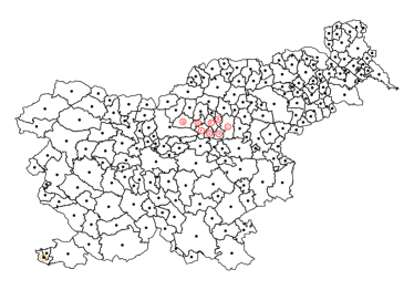
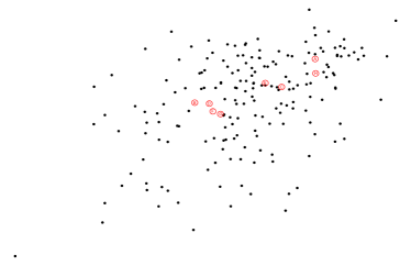
Figure 2: (a) Original Slovenia map with their areas’ centroids. (b) New centroids after projecting the original centroids coordinates into the vector space orthogonal to the columns of ${\boldsymbol{X}}$.

To define the edges of the $\mathcal{G}^{\perp}$ neighborhood structure, we consider two alternatives: 1) to use the number of neighbors $k_{i}$ of each area in the original graph (Knn); 2) to use the Delaunay triangulation to automatically define the number of neighbors. In the first method, we add edges between areas $i$ and $j$ if area $j$ is among the $k_{i}$ nearest neighbors of area $i$ in the new geography. In the second method, a Delaunay triangulation is performed over the new centroids and the vertices connected by the triangles’ edges are considered neighbors. To choose between these two methods, we analysed their ability to reproduce the true and original map adjacency structure. After all, when ${\boldsymbol{X}}$ is uncorrelated with ${\boldsymbol{\theta}}$, we expect to see only small changes in the spatial relationship between the areas. Table 1 shows the result of using the two methods in two sets of maps. The first one is composed by the 48 maps of counties from the US states but Alaska and Hawaii. The second one is composed by 26 maps of counties (indeed, municipalities) of Brazilian states. In each state, we calculate the sensitivity (or precision) of each method: the proportion of neighboring pairs of counties in the original state map that is reproduced into either the Delaunay or Knn neighborhood map in the new geography. Table 1 shows the average sensitivity over all states in US and Brazil. We also calculate the recall of each method: the proportion of neighboring pairs of counties in the reconstructed adjacency structure that is also a neighboring pair in the original map. The higher the better for both, sensitivity and recall. It is clear from the table that the Knn method is preferred according to this criterion and, from now on, all analysis in this manuscript is performed using the Knn method.

Table 1: Percentage agreement in the zero-one pattern between the original graph precision matrix and the projected precision matrices.

	Sensitivity		Recall
	Delaunay	Knn	Delaunay	Knn
U.S. counties	91.9	96.1	80.7	85.3
Brazil counties	91.9	96.7	80.5	86.6

The new adjacency matrix generated by the Knn method replaces the original adjacency matrix used in the SGLMM model. After that, the user can select his preferred algorithm to fit the model and carry out inference. For example, he can use the INLA (Rue et al., 2009) algorithm in order to take advantages of the Markov properties of the new matrix ${\boldsymbol{Q}}$ generated by the projected graph and to avoid traditional MCMC convergence problems. Although, we use INLA to perform our analysis in this paper, this is not a restriction and other software such as WinBUGS (Lunn et al., 2000), spBayes (Finley et al., 2007), OpenBUGS (Lunn et al., 2009), or CarBayes (Lee, 2013) can be used to adjust SPOCK with the ICAR or any other prior model for the spatial random effects available.

To better visualize the impact of different spatial trends in the projected graph we revisit the Slovenia map example in Figure 3 where the map is now centered at the origin $(0,0)$ and presents its original neighboring structure. For all areas, we keep the $k_{i}$ number of neighbors in the original map to reconstruct the Knn neighboring structure of the projected geography. Different spatial trends are created for one explanatory variable ${\boldsymbol{X}}$. Figure 3 is associated with a single covariate given by $X_{i}=s_{1i}+s_{2i}$, a linear trend based on the centroids’ coordinates. Figure 3 has $X_{i}=s_{1i}^{2}+s_{2i}^{2}$, while Figure 3 has $X_{i}=s_{1i}^{3}+s_{2i}^{3}$.

The original centroids are projected into the space generated by ${\boldsymbol{P}}^{\bot}$. We do not show this new geography but rather, in Figure 3, we show the original map with each $i$-th centroid connected to its new $k_{i}$ neighbors in the projected space. Although there is some overlap between segments connecting the new neighbors, we can see that each area in Figure 3 has all its $k_{i}$ neighbors approximately in the $(1,1)$ direction. As $X_{i}=(1,1)(s_{i1},s_{i2})^{\top}$, it explains the $Y$ variation in the $(1,1)$ direction and so, for the spatial effect, it remains to explain the $Y$ variation in the orthogonal $(-1,1)$ direction. In the new geography, far away areas (and therefore, with practically independent spatial effects) are those distant in the $(-1,1)$ direction. Hence, the new neighborhood structure must be the $k_{i}$ nearest neighbors in the $(1,1)$ direction. When ${\boldsymbol{X}}$ has a quadratic spatial trend, Figure 3, there is almost no effect on the projected centroids. This happens because ${\boldsymbol{X}}$ has no linear association with ${\boldsymbol{s}}$ and thus no confounding correction is necessary. We do not present in the figure, but this pattern is very similar to that when ${\boldsymbol{X}}$ is randomly generated (without any spatial pattern). Finally, Figure 3 presents a cubic pattern for ${\boldsymbol{X}}$. In this case, although not perfect as in Figure 3, there is some linear association between ${\boldsymbol{X}}$ and ${\boldsymbol{s}}$ and therefore some correction is needed. From Figure 3, it is clear that different spatial trends generates different effects over the projected graph. This is expected since the projected graph should be orthogonal to the information in the span of ${\boldsymbol{X}}$.

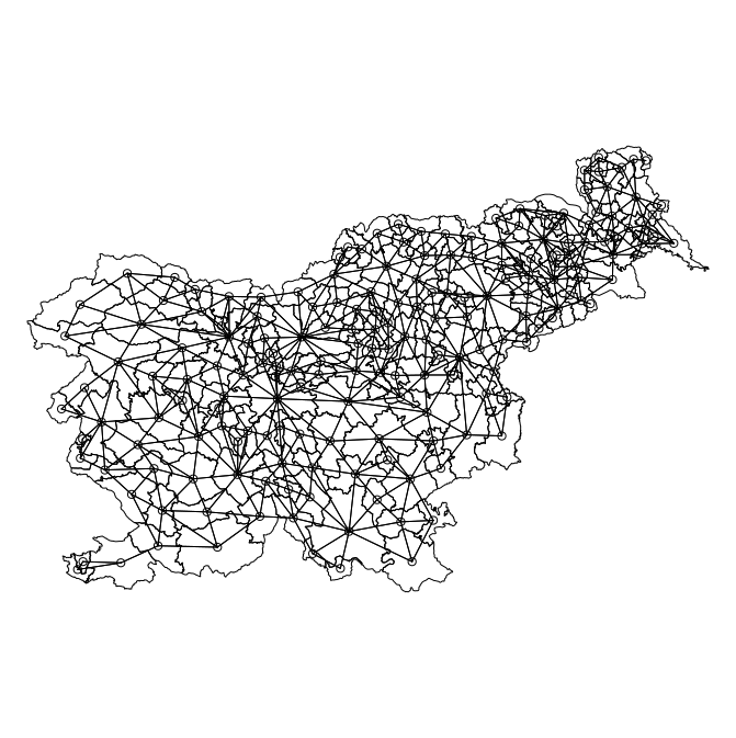
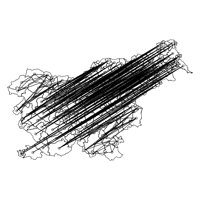
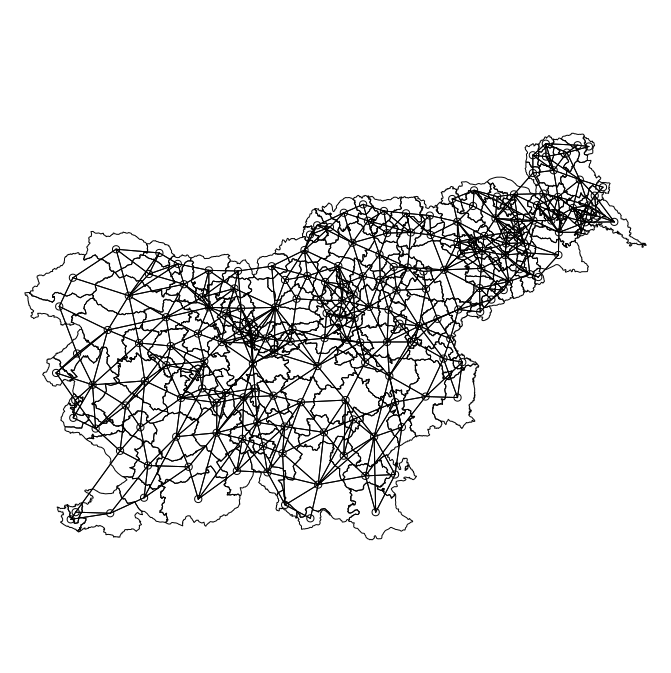
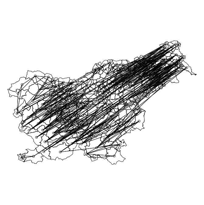
Figure 3: (a) Original Slovenia map. (b) Reconstructed adjacency matrix when ${\boldsymbol{X}}$ is a linear trend of the centroids coordinates. (c) Reconstructed adjacency matrix when ${\boldsymbol{X}}$ is a quadratic trend of the centroids coordinates (d) Reconstructed adjacency matrix when ${\boldsymbol{X}}$ is a cubic trend of the centroids coordinates.

4 When do we need to correct for spatial confounding?

An additional advantage of the SPOCK approach is to provide a diagnostic tool for detecting the need for spatial confounding correction. Statisticians would prefer to use the traditional SGLMM rather than the set of new methods to deal with spatial confounding, unless it is really necessary. As we saw in Figure 3, when ${\boldsymbol{X}}$ has no linear association with the spatial coordinates, our methodology has no effect on the geography. This could lead one to think that we should always correct for spatial confounding as an insurance policy. However, there is a clear price in using the methods that correct for spatial confounding. They are more complex and harder to interpret by epidemiologists and public health agents (Hanks et al., 2015). Next, we provide a tool based on canonical correlation to decide either one should do the confounding correction or not.

To verify the degree of linear association between the covariates ${\boldsymbol{X}}$ and the centroids ${\boldsymbol{s}}$, we apply the canonical correlation technique (Johnson et al., 1992) which measures how much variability the two sets share and if they have some common linear dimensions.

The basic idea of the the technique is to find two linear combinations ${\boldsymbol{U}}={\boldsymbol{s}}{\boldsymbol{a}}$ and ${\boldsymbol{V}}={\boldsymbol{X}}{\boldsymbol{b}}$, where ${\boldsymbol{a}}$ and ${\boldsymbol{b}}$ are $2\times 1$ and $q\times 1$, respectively, such that the correlation between ${\boldsymbol{U}}$ and ${\boldsymbol{V}}$ is maximized. The solution leads to a maximum correlation given by $\rho$, the largest eigenvalue of the matrix ${\boldsymbol{S}}^{-1/2}_{ss}{\boldsymbol{S}}_{sx}{\boldsymbol{S}}^{-1}_{xx}{\boldsymbol{S}}_{xs}{\boldsymbol{S}}^{-1/2}_{ss}$, where

$${\boldsymbol{S}}=\left[\begin{array}[]{cc}{\boldsymbol{S}}_{ss}&{\boldsymbol{S}}_{sx}\\ {\boldsymbol{S}}_{xs}&{\boldsymbol{S}}_{xx}\end{array}\right]$$

is the empirical covariance matrix of $[{\boldsymbol{s}},{\boldsymbol{X}}]$.

The need for confounding correction is based on a statistical test of the null hypothesis that $\rho=0$. There are two possible approaches, one based on an asymptotic test and another based on a Monte Carlo test.

The asymptotic test is based on the Wilks’ Lambda statistic $\Lambda$, which asymptotically has a distribution F (Wilks, 1935). This statistic is a multivariate generalization of the coefficient of determination. The basic idea is to fit a multivariate regression model where the multivariate response variable is ${\boldsymbol{s}}$ and the covariates are composed by ${\boldsymbol{X}}$. The test statistic measures the proportion of the ${\boldsymbol{s}}$ variability that can not be explained by the predictors in ${\boldsymbol{X}}$. If this value is small, we have evidence that there is a linear relationship between the two data sets. Under the normality assumption for the two matrices, ${\boldsymbol{s}}$ and ${\boldsymbol{X}}$, or if we have a large number of observations, we have $\Lambda$ following approximately an $F$ distribution. In cases where these assumptions are not valid, we carry out a randomization test by randomly permuting the rows of either ${\boldsymbol{s}}$ or ${\boldsymbol{X}}$.

5 Simulation

A simulation study is performed with two main goals: 1) to compare the results of the SPOCK methodology with the existing RHZ and HH alternative models, 2) to understand and discuss what are the models assumptions, when it is necessary to correct for spatial confounding, and what we can obtain from it. The following model is selected to generate the data:

$$Y_{i} = \beta_{0}+\beta_{1}X_{1i}+\beta_{2}X_{2i}+\theta_{i}+e_{i}$$

$$e_{i} \stackrel{{\scriptstyle ind}}{{\sim}} N(0,\tau_{e})\quad\quad i=1,\ldots,n$$

where ${\boldsymbol{\theta}}$ is the spatial effect, $n$ is the number of regions in the study. The coefficients values are ${\boldsymbol{\beta}}^{\top}=(2,1,-1)$. We selected 3 simulation scenarios:

1. (ICAR spatial-$X$) The spatial effect is generated using the ICAR structure (that is, ${\boldsymbol{\theta}}\sim N(0,\tau_{\theta}{\boldsymbol{Q}})$) with $X_{1i}$ generated from independent standard normal distribution and $X_{2i}=s_{i1}$ being the first coordinate of $i$-th area centroid;

2. (RHZ) The spatial random effect is generated by the orthogonal RHZ proposal: ${\boldsymbol{\theta}}\sim N(0,\tau_{\theta}{\boldsymbol{P}}^{\bot}{\boldsymbol{Q}}({\boldsymbol{P}}^{\bot})^{\top})$. The explanatory variables are the same as in 1;

3. (ICAR non-spatial-$X$) Its is equal to scenario 1 except that the explanatory variable $X_{2i}$ is also generated from independent standard normal distribution without any spatial information.

For each scenario, we generated 1000 datasets with the following combination of $\tau_{\theta}$ and $\tau_{e}$, the precision of the random effects and error term, respectively:

1. $\tau_{e}=0.2$ and $\tau_{\theta}=1$;

2. $\tau_{e}=1$ and $\tau_{\theta}=1$;

3. $\tau_{e}=1$ and $\tau_{\theta}=0.2$,

to study their effects in model estimation and execution time. For each of the resulting nine scenarios, the posterior estimates of the following models were recorded: 1) SPOCK, 2) RHZ, 3) HH, 4) ICAR, 5)linear model (LM), as well as their execution time. The R software (R Development Core Team, 2011) was used to fit all proposed models. For the RHZ model, we used the R script freely available in http://www4.stat.ncsu.edu/~reich/Code/. The HH model was fitted using the R package ngspatial (Hughes and Cui, 2013, version 1.02). Finally, to fit the LM, ICAR, and SPOCK models, the R-INLA package (Rue et al., 2009) was used.

We estimate the posterior mean of the fixed effects in each one of the 1000 replications. Table 2 presents the median and $2.5\%$ and $97.5\%$ percentiles of these estimates. We can see that, for all scenarios, the SPOCK model provides very similar inference compared to the LM, RHZ, and HH models. The ICAR model has a slightly different behavior. When the true generating model is the ICAR spatial-$X$, the ICAR model apparently outperforms the other models as $\tau_{\theta}$ decreases. However, this is not so simple, as we explain soon. In the RHZ scenario, the ICAR model clearly has a large variance associated with $\beta_{2}$, specially when $\tau_{\theta}=0.2$. This is expected because, as Reich et al. (2006) show, as the ratio $\tau_{\theta}/\tau_{e}$ decreases, the confounding problem becomes severe. Finally, in the ICAR non-spatial-$X$ scenario, with no spatial information in the explanatory variables, all models seem to present a similar behavior, independently of precision differences.

Table 2: Median summary of the posterior mean estimate from 1000 replicates in the simulation setting. The brackets contain the $2.5\%$ and $97.5\%$ posterior percentiles of fixed effects estimates in 1000 replicates.

		Scenario
		ICAR spatial-$X$			RHZ			ICAR non-spatial-$X$
$\tau_{e},\tau_{\theta}$	Model	$\beta_{0}$	$\beta_{1}$	$\beta_{2}$	$\beta_{0}$	$\beta_{1}$	$\beta_{2}$	$\beta_{0}$	$\beta_{1}$	$\beta_{2}$
True		2	1	$-$1	2	1	$-$1	2	1	$-$1
	SPOCK	2.00 (1.69, 2.31)	1.00 (0.66, 1.32)	-0.99 (-1.80, -0.12)	2.00 (1.69, 2.31)	1.00 (0.67, 1.31)	-1.00 (-1.30, -0.67)	2.00 (1.69, 2.31)	1.00 (0.65, 1.32)	-1.00 (-1.29, -0.62)
	RHZ	2.00 (1.69, 2.31)	1.00 (0.66, 1.32)	-0.99 (-1.80, -0.11)	2.00 (1.69, 2.31)	1.00 (0.67, 1.31)	-1.00 (-1.30, -0.67)	2.00 (1.69, 2.31)	1.00 (0.66, 1.32)	-1.00 (-1.29, -0.68)
$0.2,1$	HH	2.00 (1.69, 2.31)	1.00 (0.66, 1.32)	-1.02 (-1.84, -0.13)	2.00 (1.69, 2.31)	1.00 (0.67, 1.31)	-1.00 (-1.30, -0.67)	2.00 (1.69, 2.31)	1.00 (0.65, 1.32)	-1.00 (-1.30, -0.67)
	ICAR	2.00 (1.69, 2.31)	1.00 (0.66, 1.32)	-1.00 (-1.76, -0.18)	2.00 (1.69, 2.31)	1.00 (0.67, 1.30)	-1.00 (-1.46, -0.46)	2.00 (1.69, 2.31)	1.00 (0.66, 1.33)	-1.00 (-1.29, -0.68)
	LM	2.00 (1.69, 2.31)	1.00 (0.66, 1.32)	-0.99 (-1.80, -0.12)	2.00 (1.69, 2.31)	1.00 (0.67, 1.31)	-1.00 (-1.30, -0.67)	2.00 (1.69, 2.31)	1.00 (0.65, 1.32)	-1.00 (-1.29, -0.68)
	SPOCK	2.00 (1.86, 2.14)	1.00 (0.83, 1.16)	-1.01 (-1.74, -0.18)	2.00 (1.86, 2.14)	1.00 (0.85, 1.14)	-1.00 (-1.14, -0.85)	2.00 (1.86, 2.14)	1.00 (0.83, 1.16)	-1.00 (-1.15, -0.84)
	RHZ	2.00 (1.86, 2.14)	1.00 (0.84, 1.16)	-1.01 (-1.75, -0.17)	2.00 (1.86, 2.14)	1.00 (0.85, 1.14)	-1.00 (-1.13, -0.85)	2.00 (1.86, 2.14)	1.00 (0.82, 1.16)	-0.99 (-1.16, -0.83)
$1,1$	HH	2.00 (1.86, 2.14)	1.00 (0.84, 1.16)	-1.01 (-1.81, -0.20)	2.00 (1.86, 2.14)	1.00 (0.85, 1.14)	-1.00 (-1.13, -0.85)	2.00 (1.86, 2.14)	1.00 (0.83, 1.16)	-1.00 (-1.16, -0.83)
	ICAR	2.00 (1.86, 2.14)	1.00 (0.85, 1.16)	-1.01 (-1.63, -0.29)	2.00 (1.86, 2.14)	1.00 (0.84, 1.15)	-1.00 (-1.48, -0.47)	2.00 (1.86, 2.14)	1.00 (0.84, 1.16)	-1.00 (-1.14, -0.85)
	LM	2.00 (1.86, 2.14)	1.00 (0.84, 1.16)	-1.01 (-1.75, -0.17)	2.00 (1.86, 2.14)	1.00 (0.85, 1.14)	-1.00 (-1.13, -0.85)	2.00 (1.86, 2.14)	1.00 (0.83, 1.16)	-0.99 (-1.16, -0.83)
	SPOCK	2.00 (1.86, 2.14)	1.00 (0.76, 1.24)	-1.01 (-2.68, 0.73)	2.00 (1.86, 2.14)	1.00 (0.84, 1.14)	-1.00 (-1.14, -0.83)	2.00 (1.86, 2.14)	1.00 (0.75, 1.22)	-1.00 (-1.23, -0.76)
	RHZ	2.00 (1.86, 2.14)	1.00 (0.76, 1.23)	-0.99 (-2.68, 0.77)	2.00 (1.86, 2.14)	1.00 (0.85, 1.14)	-1.00 (-1.13, -0.85)	2.00 (1.86, 2.14)	1.00 (0.73, 1.24)	-0.99 (-1.26, -0.74)
$1,0.2$	HH	2.00 (1.86, 2.14)	1.00 (0.77, 1.23)	-0.99 (-2.79, 0.76)	2.00 (1.86, 2.14)	1.00 (0.85, 1.14)	-1.00 (-1.13, -0.85)	2.00 (1.86, 2.14)	1.00 (0.76, 1.25)	-1.00 (-1.26, -0.73)
	ICAR	2.00 (1.86, 2.14)	1.00 (0.81, 1.20)	-1.01 (-2.28, 0.36)	2.00 (1.86, 2.14)	1.00 (0.80, 1.19)	-1.03 (-2.20, 0.25)	2.00 (1.86, 2.14)	1.00 (0.80, 1.21)	-1.00 (-1.19, -0.80)
	LM	2.00 (1.86, 2.14)	1.00 (0.76, 1.23)	-0.99 (-2.68, 0.77)	2.00 (1.86, 2.14)	1.00 (0.85, 1.14)	-1.00 (-1.13, -0.85)	2.00 (1.86, 2.14)	1.00 (0.73, 1.24)	-0.99 (-1.26, -0.74)

From Table 2, we can get two main conclusions. First, there is no major differences in the estimates provided by the SPOCK and the RHZ or HH models, making it a competitive model. The difference on the fitted parameters between the ICAR model and the other three models is large when the ratio between the spatial effect precision and the error precision is small ($\tau_{\theta}/\tau_{e}=0.2$). The second one, is the apparent better behavior of the ICAR model in the ICAR spatial-$X$ scenario. We discuss that this is not necessarily so in the following.

Hodges and Reich (2011) discuss the interpretation of confounding in spatial regression and link it with the multicollinearity problem in linear regression. By construction, the solution proposed by Reich et al. (2006) and more recently by Hughes and Haran (2013) assigns to ${\boldsymbol{X}}$ all the spatial variation that ${\boldsymbol{\theta}}$ and ${\boldsymbol{X}}$ are competing for. That is, RHZ, HH and our own method aims to estimate

$${\boldsymbol{\beta}}^{*}=\left({\boldsymbol{\beta}}+\left({\boldsymbol{X}}^{\top}{\boldsymbol{X}}\right)^{-1}{\boldsymbol{X}}^{\top}[{\boldsymbol{1}},{\boldsymbol{s}}_{1},{\boldsymbol{s}}_{2}]{\boldsymbol{\gamma}}\right)$$

in (10). There is not an universal agreement around this solution. Paciorek (2010) and Hanks et al. (2015) argue that this is a very strong assumption to alleviate the confounding problem by making the spatial random effects orthogonal to the space of the span of ${\boldsymbol{X}}$.

In non-spatial linear models with two covariates $X$ and $Z$ and the presence of multicollinearity, a possible solution arises when one has an intrinsic interest on the causal effect of $X$ and $Z$ appears only as nuisance. In this case, we can regress $Z$ in $X$ and use the regression residual $Z^{\bot}$ as a covariate instead of $Z$. This situation is exactly what happens in the spatial regression problem when you do not want to “mess up the fixed effect you love” (Hodges and Reich, 2011). Indeed, in this problem, most of the time, the spatial effect ${\boldsymbol{\theta}}$ has the same role as $Z$ and it is only a nuisance error representing unobserved spatially structured variables. The covariates in ${\boldsymbol{X}}$ represent truly relevant factors with possible causality. This is the rationale to estimate ${\boldsymbol{\beta}}^{*}$ rather than ${\boldsymbol{\beta}}$ and it motivates the RHZ, HH, and SPOCK models to alleviate the spatial confounding.

A better understanding of the effects of alleviating confounding must be investigated looking at the differences between the $\hat{{\boldsymbol{\beta}}}$ Bayesian estimate (posterior mean) and ${\boldsymbol{\beta}}^{*}$, rather than ${\boldsymbol{\beta}}$. To investigate this issue, we produce Figure 4. We calculate the ratio $\hat{{\boldsymbol{\beta}}}/{\boldsymbol{\beta}}^{*}$ in each one of the 1000 simulations and show them in the box plots for the 3 scenarios with $\tau_{\theta}=0.2$ and $\tau_{e}=1$ fixed. Similar figures appear with the other values for $\tau_{\theta}$ and $\tau_{e}$. Each scenario is shown in a different column. The first and second rows of plots present $\hat{\beta}_{0}/\beta^{*}_{0}$ and $\hat{\beta}_{1}/\beta^{*}_{1}$, respectively. Their coefficients $\beta_{0}$ and $\beta_{1}$ are not associated with spatial covariates. They have a similar behavior in all scenarios and the main conclusion is that the different methods produce very similar results. The third row presents the distribution of the ratio $\hat{\beta}_{2}/\beta^{*}_{2}$. The first two scenarios, ICAR spatial-$X$ and RHZ, have $\beta_{2}$ associated with a covariate with spatial structure. In this case, the traditional ICAR method has a much larger variance than the methods that alleviate spatial confounding. This shows that the ICAR method is not a good choice when the aim is to assign to ${\boldsymbol{X}}$ all the variation in ${\boldsymbol{\theta}}$ that is shared with it. In the ICAR non-spatial-$X$ scenario, all methods return to have a similar behavior, as expected.

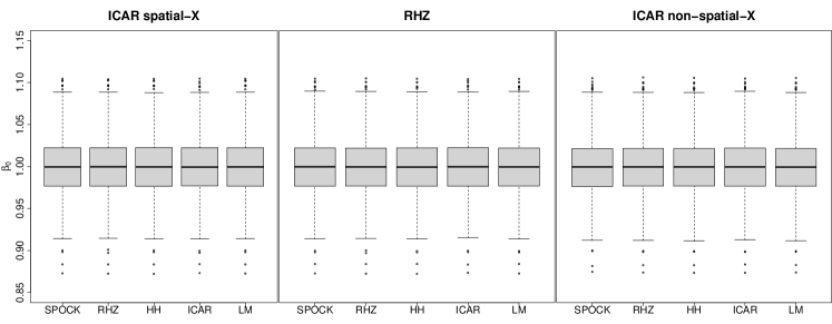
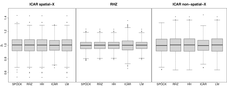
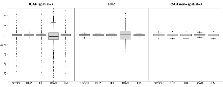
Figure 4: (a) Posterior estimates for $\beta_{0}$ under the different models. (b) Posterior estimates for $\beta_{1}$ under the different models. (c) Posterior estimates for $\beta_{2}$ under the different models.

After demonstrating that the SPOCK model is capable of removing the spatial confounding and of providing very similar results to RHZ and HH models, we evaluate the average time to run each method. Table 3 presents the median execution time of 1000 replicates of each model for scenario RHZ. The LM method is substantially faster than the others. However, the LM method does not take into account the spatial variation that improves modeling. Among the spatial models, SPOCK clearly outperforms the RHZ and HH methods in running time and it has comparable time with the ICAR model. The RHZ has the largest median time, while the HH method seems to perform around 10 times slower than SPOCK.

Table 3: Median execution time (in seconds) from 1000 replicates in scenario 2 (RHZ) and the execution standard deviation (sd) of the evaluation time of each method.

$\tau_{e},\tau_{\theta}$	Model	Time (sec)	sd
	SPOCK	1.850	0.10
	RHZ	157.006	0.92
$0.2,1$	HH	19.157	3.38
	ICAR	0.597	0.09
	LM	0.257	0.02
	SPOCK	1.872	0.09
	RHZ	157.152	0.62
$1,1$	HH	18.116	3.66
	ICAR	0.573	0.04
	LM	0.261	0.02
	SPOCK	1.879	0.10
	RHZ	158.254	1.43
$1,0.2$	HH	20.898	3.67
	ICAR	0.582	0.04
	LM	0.259	0.02

6 Slovenia Data

The proposed model was adjusted to the same dataset used by Reich et al. (2006). The response variable $Y_{i}$ is the number of cases of stomach cancer observed in the municipalities of Slovenia during the 1995-2001 period. The single covariate is the standardized value of a socioeconomic status measure for each area $i=1,\ldots,192$. Therefore, we have the following model:

$$Y_{i}|\lambda_{i}, \sim \mbox{Poisson}(\lambda)$$

$$\log(\lambda_{i}) = {\boldsymbol{X}}_{i}{\boldsymbol{\beta}}+\theta_{i}$$

with ${\boldsymbol{\beta}}$ the fixed effect and ${\boldsymbol{\theta}}$ the spatial effect.

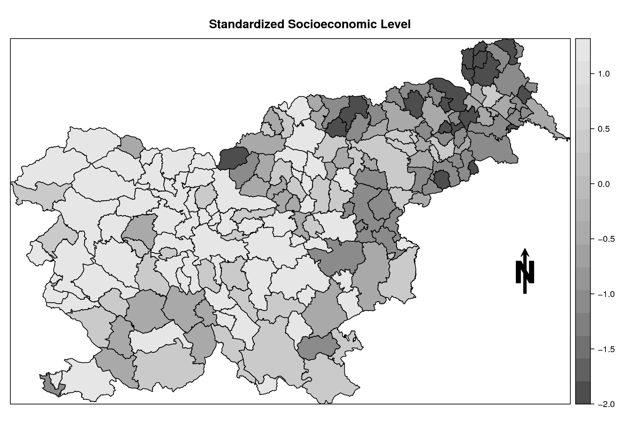
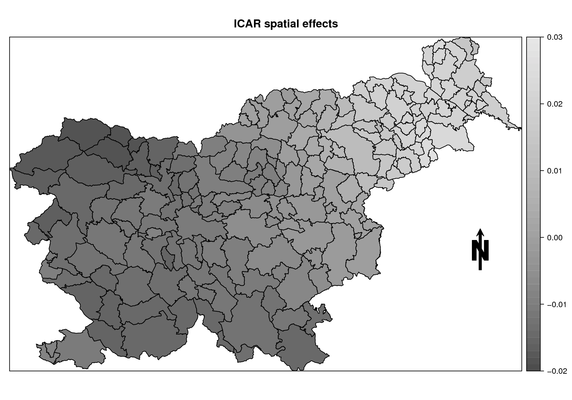
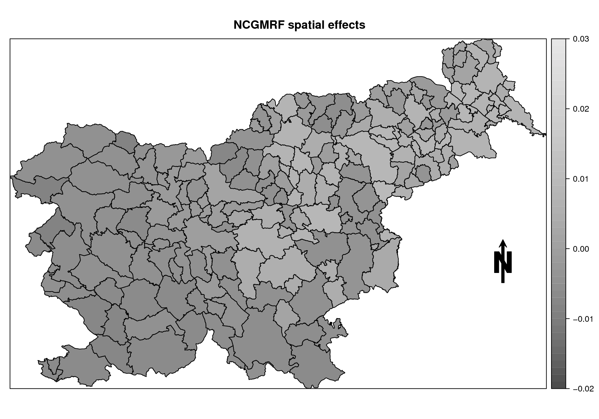
Figure 5: (a) Standardized socioeconomic level for the municipalities of Slovenia. (b) Posterior mean estimates for spatial random effects of the ICAR model. (c) Posterior mean estimates for spatial random effects of the SPOCK model

Using a simple exploratory analysis, the authors noticed that the data show a negative relationship between the response and the explanatory variable. This is expected based on the common knowledge of association between health risk and deprivation. Their first attempt was to fit the data with the traditional SGLMM to capture the spatial heterogeneity. However, from Figure 5, it is clear that the explanatory variable have a diagonal spatial trend presenting higher values in the southwest and smaller in the northeast. This is an indication of the presence of confounding between the random spatial effects and the socioeconomic level. The pattern in this dataset is similar to what we simulated in Section 3 when we took $X_{i}=s_{i1}+s_{i2}$ (see Figure 3). After the SGLMM model was fitted by Reich et al. (2006), the coefficient associated with socioeconomic level had a very wide credibility interval that covered even positive values. That is, the covariate negative effect disappeared.

Using our diagnosis test from Section 4, we can verify if there will be, in fact, a confounding effect. Calculating the first canonical correlation between the spatial centroids ${\boldsymbol{s}}$ and the covariate ${\boldsymbol{X}}$, we find it equal to 0.67. This value is highly significant according to both, the asymptotic and a permutation test, obtained from Menzel (2012). The value is also high in absolute terms, indicating that the random spatial effects will be mixed up with the covariate effects.

To better understand the confounding effect between the exploratory variable and the random effects, we look at the spatial residuals from the ICAR model. From Figure 5, it is clear that both, the spatial random effect and the explanatory variable, share a southwest to northeast trend and therefore are competing for the spatial variability contained in the response $Y_{i}$. Figure 5 show the posterior mean estimates for the spatial effects under our SPOCK model. After alleviating the spatial confounding, there still is some spatial trend left in the same direction southwest to northeast. However, the spatial dependence now is weaker and the spatial effects are smoothed toward zero. This is expected since after alleviating the spatial confounding we assume that the exploratory variable carries most of the spatial information in $Y_{i}$. Although weaker, it is important to notice that the spatial random effect structure from the SPOCK model is still coherent with the space under analysis.

Table 4 shows the posterior mean estimates and credible intervals obtained applying all discussed models. The SPOCK point estimate and credible interval is similar to the RHZ and HH models. However, as it can be seen in the last column of Table 4, time wise SPOCK drastically outperforms the non-confounding methods.

Model	$\beta_{Se}$	95% Credible Interval	Time (sec)
SPOCK	$-$0.1004	($-$0.1635, $-$0.0369)	2.21
RHZ	$-$0.1137	($-$0.1688, $-$0.0596)	251.83
HH	$-$0.1128	($-$0.1656, $-$0.0450)	29.39
ICAR	$-$0.0474	($-$0.1404, 0.0473)	0.73
LM	$-$0.0682	($-$0.1067, $-$0.0298)	0.16

Table 4: Posterior mean estimate and credible intervals of the coefficient associated with the socioeconomic variable (Se) for the five fitted models.

7 Conclusion

In this paper we introduced an alternative way to alleviate spatial confounding. The main idea is to construct a graph capable of capturing the spatial dependence orthogonal to the space generated by the span of ${\boldsymbol{X}}$. By doing so, the introduced method maintains the original sparsity of the precision matrix ${\boldsymbol{Q}}$ and introduces no restriction in the spatial modeling setup.

From our simulation study and real data example, we were able to show that the SPOCK approach provides similar results to the others methods that alleviate confounding. These alternative models project the spatial random effects on the orthogonal space spanned by ${\boldsymbol{X}}$. Instead, SPOCK projects the original graph $\mathcal{G}$ on that same vector space. In all simulated scenarios, our method was at least 10 times faster than the existing methodologies. This advantage can make it more attractive to researchers in different areas. Another advantage is that our method can be used with any usual ICAR implementation such as INLA, WinBUGS, spBayes, OpenBUGS, and CarBayes.

We showed that, when no spatial confounding is present, it does not matter which method one uses. However, when this is not the case, running an usual ICAR or the spatial alleviating methods may result in different coefficients and inference. The right question is not which approach is the correct one. Each of them estimates a different parameter, ${\boldsymbol{\beta}}$ or ${\boldsymbol{\beta}}^{*}$. Specific application considerations should guide which parameter is more meaningful. In the common situation where the spatial effects ${\boldsymbol{\theta}}$ represent geographically structured nuisance effects, it may be desirable to assign to ${\boldsymbol{X}}$ all linear spatial variation that is present in ${\boldsymbol{\theta}}$ and hence, to estimate ${\boldsymbol{\beta}}^{*}$. However, as mentioned by Paciorek (2010), the data generating system may have a non-observed spatial confounder with the observed explanatory variables and setting all spatial variation to the observed covariates may not be appropriate.

The SPOCK methodology allow for the proposal of a diagnostic test that can help on deciding when we should carry out the correction for spatial confounding. It is simple and can be calculated previous to any model fitting. When there is no spatial confounding, fitting ICAR will lead to the same inference as the spatial confounding alleviating methods as ${\boldsymbol{\beta}}$ and ${\boldsymbol{\beta}}^{*}$ are the same. However, fitting ICAR in the other situation, when there is unobserved spatial confounders, leads to an estimate of ${\boldsymbol{\beta}}$, rather than of ${\boldsymbol{\beta}}^{*}$. The user should be aware of these differences so he does not use one thinking to have the other.

References

- Besag (1974) Besag, J. (1974), “Spatial Interaction and the Statistical Analysis of Lattice Data Systems (with discussion),” Journal of the Royal Statistical Society, Series B, 36, 192–225.
- Besag et al. (1991) Besag, J., York, J., and Mollie, A. (1991), “Bayesian Image Restoration with Two Application in Spatial Statistics (with discussion),” Annals of the Institute Statistical Mathematics, 43, 1–59.
- Clayton et al. (1993) Clayton, D., Bernardinelli, L., and Montomoli, C. (1993), “Spatial correlation in ecological analysis,” International Journal of Epidemiology, 6, 1193–1202.
- Finley et al. (2007) Finley, A. O., Banerjee, S., and Carlin, B. P. (2007), “spBayes: An R Package for Univariate and Multivariate Hierarchical Point-referenced Spatial Models,” Journal of Statistical Software, 19, 1–24.
- Hanks et al. (2015) Hanks, E. M., Schliep, E. M., Hooten, M. B., and Hoeting, J. A. (2015), “Restricted spatial regression in practice: geostatistical models, confounding, and robustness under model misspecification,” Environmetrics, 26, 243–254.
- Hodges and Reich (2011) Hodges, J. S. and Reich, B. J. (2011), “Adding Spatially-Correlated Errors Can Mess Up the Fixed Effect You Love,” The American Statistician, 64, 325–334.
- Hughes and Cui (2013) Hughes, J. and Cui, X. (2013), ngspatial: Classes for Spatial Data, Minneapolis, MN, r package version 1.0-2.
- Hughes and Haran (2013) Hughes, J. and Haran, M. (2013), “Dimension reduction and alleviation of confounding for spatial generalized linear mixed models,” Journal of the Royal Statistical Society, Series B, 75, 139–159.
- Johnson et al. (1992) Johnson, R. A., Wichern, D. W., et al. (1992), Applied multivariate statistical analysis, vol. 4, Prentice hall Englewood Cliffs, NJ.
- Lavine and Hodges (2012) Lavine, M. L. and Hodges, J. S. (2012), “On rigorous specification of ICAR models,” The American Statistician, 66, 42–49.
- Lee (2013) Lee, D. (2013), “CARBayes: An R Package for Bayesian Spatial Modeling with Conditional Autoregressive Priors,” Journal of Statistical Software, 55, 1–24.
- Leroux et al. (1999) Leroux, B. G., Lei, X., and Breslow, N. (1999), “Estimation of Disease Rates in Small Areas: A New Mixed Model for Spatial Dependence,” in In Statistical Models in Epidemiology; the Environment and Clinical Trials, eds. Halloran, M. E. and Berry, D., New York: Springer–Verlag, pp. 179–192.
- Lunn et al. (2009) Lunn, D., Spiegelhalter, D., Thomas, A., and Best., N. (2009), “The BUGS project: Evolution, critique and future directions (with discussion),” Statistics in Medicine, 28, 3049–3082.
- Lunn et al. (2000) Lunn, D. J., Thomas, A., Best, N., and Spiegelhalter, D. (2000), “WinBUGS – a Bayesian modelling framework: Concepts, structure, and extensibility,” Statistics and Computing, 10, 325–337.
- Menzel (2012) Menzel, U. (2012), CCP: Significance Tests for Canonical Correlation Analysis (CCA), r package version 1.1.
- Mosteller and Tukey (1997) Mosteller, F. and Tukey, J. W. (1997), Data analysis and regression, Reading: Addison-Wesley.
- Murakami and Griffith (2015) Murakami, D. and Griffith, D. A. (2015), “Random effects specifications in eigenvector spatial filtering: a simulation study,” Journal of Geographical Systems, 17, 311–331.
- Paciorek (2010) Paciorek, C. J. (2010), “The Importance of Scale for Spatial-Confounding Bias and Precision of Spatial Regression Estimators,” Statistical Science, 25, 107–125.
- R Development Core Team (2011) R Development Core Team (2011), R: A Language and Environment for Statistical Computing, R Foundation for Statistical Computing, Vienna, Austria, ISBN 3-900051-07-0.
- Reich et al. (2006) Reich, B. J., Hodges, J. S., and Zadnik, V. (2006), “Effects of Residual Smoothing on the Posterior of the Fixed Effects in Disease-Mapping Models,” Biometrics, 62, 1197–1206.
- Rodrigues and Assunção (2012) Rodrigues, E. C. and Assunção, R. (2012), “Bayesian spatial models with a mixture neighborhood structure,” Journal of Multivariate Analysis, 109, 88 – 102.
- Rue and Held (2005) Rue, H. and Held, L. (2005), Gaussian Markov random fields: Theory and applications, Chapman & Hall.
- Rue et al. (2009) Rue, H., Martino, S., and Chopin, N. (2009), “Approximate Bayesian Inference for Latent Gaussian Models Using Integrated Nested Laplace Approximations (with discussion),” Journal of the Royal Statistical Society, Series B, 71, 319–392.
- Wilks (1935) Wilks, S. (1935), “On the independence of k sets of normally distributed statistical variables,” Econometrica, Journal of the Econometric Society, 309–326.
- Zadnik and Reich (2006) Zadnik, V. and Reich, B. J. (2006), “Analysis of the relationship between socioeconomic factors and stomach cancer incidence in Slovenia,” Neoplasma, 53, 103–110.