Hypothesis Testing For Network Data
in Functional Neuroimaging

Abstract

In recent years, it has become common practice in neuroscience to use networks to summarize relational information in a set of measurements, typically assumed to be reflective of either functional or structural relationships between regions of interest in the brain. One of the most basic tasks of interest in the analysis of such data is the testing of hypotheses, in answer to questions such as “‘Is there a difference between the networks of these two groups of subjects?” In the classical setting, where the unit of interest is a scalar or a vector, such questions are answered through the use of familiar two-sample testing strategies. Networks, however, are not Euclidean objects, and hence classical methods do not directly apply. We address this challenge by drawing on concepts and techniques from geometry, and high-dimensional statistical inference. Our work is based on a precise geometric characterization of the space of graph Laplacian matrices and a nonparametric notion of averaging due to Fréchet. We motivate and illustrate our resulting methodologies for testing in the context of networks derived from functional neuroimaging data on human subjects from the 1000 Functional Connectomes Project. In particular, we show that this global test is more statistical powerful, than a mass-univariate approach. In addition, we have also provided a method for visualizing the individual contribution of each edge to the overall test statistic.

18 blue

, , , , and

t1This work was supported by a grant from the Air Force Office for Scientific Research (AFOSR), whose grant number is FA9550-12-1-0102. t2This material is also based upon work supported by, or in part by, the U. S. Army Research Laboratory and the U. S. Army Research Office under contract/grant number W911NF1510440.

1 Introduction

Functional neuroimaging data has been central to the advancement of our understanding of the human brain. Neuroimaging data sets are increasingly approached from a graph-theoretical perspective, using the tools of modern network science (Bullmore and Sporns, 2009). This has elicited the interest of statisticians working in that area. At the level of basic measurements, neuroimaging data can be said to consist typically of a set of signals (usually time series) at each of a collection of pixels (in two dimensions) or voxels (in three dimensions). Building from such data, various forms of higher-level data representations are employed in neuroimaging. Traditionally, two- and three-dimensional images have, naturally, been the norm, but increasingly in recent years there has emerged a substantial interest in network-based representations.

1.1 Motivation

Let $G=(V,E)$ denote a graph, based on $d=|V|$ vertices. In this setting, the vertices $v\in V$ correspond to regions of interest (ROIs) in the brain, often pre-defined through considerations of the underlying neurobiology (e.g., the putamen or the cuneus). Edges $\{u,v\}\in E$ between vertices $u$ and $v$ are used to denote a measure of association between the corresponding ROIs. Depending on the imaging modality used, the notion of ‘association’ may vary. For example, in diffusion tensor imaging (DTI), associations are taken to be representative of structural connectivity between brain regions. On the other hand, in functional magnetic resonance imaging (fMRI), associations are instead thought to represent functional connectivity, in the sense that the two regions of the brain participate together in the achievement of some higher-order function, often in the context of performing some task (e.g., counting from $1$ to $10$).

With neuroimaging now a standard tool in clinical neuroscience, and with the advent of several major neuroscience research initiatives – perhaps most prominent being the recently announced Brain Research Accelerated by Innovative Neurotechnologies (BRAIN) initiative – we are quickly moving towards a time in which we will have available databases composed of large collections of secondary data in the form of network-based data objects. Faced with databases in which networks are a fundamental unit of data, it will be necessary to have in place the statistical tools to answer such questions as, “What is the ‘average’ of a collection of networks?” and “Do these networks differ, on average, from a given nominal network?,” as well as “Do two collections of networks differ on average?” and “What factors (e.g., age, gender, etc.) appear to contribute to differences in networks?”, or finally, say, “Has there been a change in the networks for a given subpopulation from yesterday to today?” In order to answer these and similar questions, we require network-based analogues of classical tools for statistical estimation and hypothesis testing.

While these classical tools are among the most fundamental and ubiquitous in use in practice, their extension to network-based datasets, however, is not immediate and, in fact, can be expected to be highly non-trivial. The main challenge in such an extension is due to the simple fact that networks are not Euclidean objects (for which classical methods were developed) – rather, they are combinatorial objects, defined simply through their sets of vertices and edges. Nevertheless, our work here in this paper demonstrates that networks can be associated with certain natural subsets of Euclidean space, and furthermore demonstrates that through a combination of tools from geometry, probability on manifolds, and high-dimensional statistical analysis it is possible to develop a principled and practical framework in analogy to classical tools. In particular, we focus on the development of an asymptotic framework for one- and two-sample hypothesis testing.

Key to our approach is the correspondence between an undirected graph $G$ and its Laplacian, where the latter is defined as the matrix $L=D-W$; with $W$ denoting the $d\times d$ adjacency matrix of $G$ and $D$ a diagonal matrix with the vertex degrees along the diagonal. When $G$ has no self-loops and no multi-edges, the correspondence between graphs $G$ and Laplacians $L$ is one-to-one. Our work takes place in the space of graph Laplacians. Importantly, this requires working not in standard Euclidean space $\mathbb{R}^{n}$, but rather on certain subsets of Euclidean space which are either submanifolds of $\mathbb{R}^{n}$, or submanifolds of $\mathbb{R}^{n}$ with corners. While these subsets of Euclidean space have the potential to be complicated in nature, we show that in the absence of any nontrivial structural constraints on the graphs $G$, the geometry of these subsets is sufficiently ‘nice’ to allow for a straightfoward definition of distance between networks to emerge.

Our goal in this work is the development of one- and two-sample tests for network data objects that rely on a certain sense of ‘average’. We adopt the concept of Fréchet means in defining what average signifies in our context. Recall that, for a metric space, $(\mathcal{X},\rho)$, and a probability measure, $Q$, on its Borel $\sigma$-field, under appropriate conditions, the Fréchet mean of $Q$ is defined as the (possibly nonunique) minimizer

$$\mu:=\operatornamewithlimits{argmin}_{x\in\mathcal{X}}\int\limits_{\mathcal{X}}\rho^{2}(x,y)Q(dy).$$ (1)

Similarly, for any sample of realizations from $Q$ on $\mathcal{X}$, denoted $Y:=\{Y_{1},\ldots,Y_{n}\}$, the corresponding sample Fréchet mean is defined as

$$\widehat{\mu}_{n}(Y):=\operatornamewithlimits{argmin}_{x\in\mathcal{X}}\frac{1}{n}\sum_{i=1}^{n}\rho^{2}(x,Y_{i}).$$ (2)

Thus, the distance $\rho$ that emerges from our study of the geometry of the space of networks implicitly defines a corresponding notion of how to ‘average’ networks.

Drawing on results from nonparametric statistical inference on manifolds, we are then able to establish a central limit theory for such averages and, in turn, construct the asymptotic distributions of natural analogues of one- and two-sample $z$-tests. These tests require knowledge of the covariance among the edges of our networks, which can be expected to be unavailable in practice. Nevertheless, we show how recent advances in the estimation of large, structured covariance matrices can be fruitfully brought to bear in our context, and provide researchers with greater statistical power than a mass-univariate approach, which is the standard approach in this field.

1.2 The 1000 Functional Connectomes Project

Our approach is motivated by and illustrated with data from the 1000 Functional Connectomes Project (FCP). This major MRI data-sharing initiative was launched in 2010 (Biswal et al., 2010). The impetus for the 1000 FCP was given by a need to make widely accessible neuroimaging data, which are costly and time-consuming to collect (Biswal et al., 2010). This was conducted within the so-called “discovery science” paradigm, paralleling similar initiatives in systems biology. The 1000 FCP constituted the largest data set of its kind, at the time of its release. As for the use of such large data sets in genetics, it is believed that facilitating access to high-throughput data generates economies of scale that are likely to lead to more numerous and more substantive research findings.

The 1000 FCP describes functional neuroimaging data from 1093 subjects, located in 24 community-based centers. The mean age of the participants is 29 years, and all subjects were 18 years-old or older. Each individual scan lasted between 2.2 and 20 minutes. The strength of the MRI scanner varied across centers, with $n=970$ scans at 3T and $n=123$ at 1.5T. Voxel-size was 1.5–5mm within the plane; and slice thickness was 3–8mm. The ethics committee in each contributing data center approved the project; and the institutional review boards of the NYU Langone Medical Center and of the New Jersey Medical School approved the dissemination of the data. This freely available data set has been extensively used in the neuroimaging literature (Yan et al., 2013; Tomasi and Volkow, 2010; Zuo et al., 2012).

The individual fMRI scans were parcellated into a set of 50 cortical and subcortical regions, using the Automated Anatomical Labeling (AAL) template (Tzourio-Mazoyer et al., 2002). Note, that that the resulting connectivity networks are sensitive to our particular choice of parcellation, and that the results in this paper need not generalize to other templates (see Wang et al., 2009, for a review). The voxel-specific time series in each of these regions were aggregated to form mean regional time series, as commonly done in the study of the human connectome (see for example Achard et al., 2006). The resulting regional time series were then compared using two different measures of association. We here considered the correlation coefficient since this measure has proved to be popular in the neuroimaging literature (Ginestet and Simmons, 2011; Pachou et al., 2008; Micheloyannis et al., 2009).

Subjects in the 1000 FCP data can be subdivided with respect to sex. Several groups of researchers have previously considered the impact of sex differences on resting-state connectivity (Biswal et al., 2010; Tomasi and Volkow, 2011). It is hypothesized that sexual dimorphism in human genomic expression is likely to affect a wide range of physiological variables (Ellegren and Parsch, 2007). In particular, differences in hormonal profiles (e.g. estrogen) during brain development are known to be related to region-specific effects (McEwen, 1999). Thus, it is of interest to compare the subject-specific networks of males and females in the 1000 FCP data set (see Figure 1). Observe that previous research in this field has established local sex differences in connectivity by considering individual edge weights (Biswal et al., 2010; Tomasi and Volkow, 2011). By contrast, we are here investigating the effect of sex differences on entire networks.

It is here useful to distinguish between these two types of network data analysis in neuroimaging. While local analysis focuses on edge-specific statistics; global analysis instead considers network topological properties such as the shortest-path length. In this paper, we are extending the latter by providing a framework for identifying the mean network, and characterizing the space of all possible such networks.

The organization of this paper is as follows. In Section 2, we describe the statistical and mathematical background of this type of research questions. In Section 3, we provide a geometrical characterization of the space of networks under scrutiny. In Section 4, we describe how certain central limit theorems can be adapted to this space, in order to construct a statistical inferential framework for network data. A simulation study exploring the relationship between statistical power and various aspects of neuroimaging data is reported in Section 5. In Section 6, we apply this framework to the analysis of a subset of the data from the 1000 FCP. These results and the potential extensions of the proposed statistical tests are then discussed in Section 7.

(A) Sex                                                (B) Age
           Female           Male                        $x\leq 22$        $22<x\leq 32$       $32<x$
                                     

Figure 1: Descriptive statistics for the 1000 FCP data set. In panel (A), the group-specific mean Laplacians for networks over 50 AAL vertices in females ($n_{f}=555$), and males ($n_{m}=462$). Similarly, in panel (B), the age variable has been divided into three groups ($n_{1}=386$, $n_{2}=297$, and $n_{3}=334$), and the respective means are reported for each age group. The Laplacians have been binarized with respect to the $75^{\text{th}}$ percentile of the overall distribution of the entries in the full 1000 FCP database. (Black indicates entries greater or equal than that percentile).

2 Related Work

At the heart of the class of statistical problems we wish to address is a desire to summarize and compare groups of network data objects in a statistically principled manner. There are, of course, already a variety of numerical devices available for carrying out certain descriptive summaries and comparisons. Basic set-theoretic operations (e.g., union, intersection, symmetric difference) are all well-defined for graphs. More broadly, various metrics, such as the Hamming distance, have been borrowed from other fields and applied to graphs. Currently, the mainstay in the analysis of network data in neuroimaging, is the mass-univariate approach in which independent tests are conducted for every edge, adjusting for multiple testing. See Ginestet, Fournel and Simmons (2014) for a survey of such methods in the context of functional neuroimaging.

Such mass-univariate approaches, however, fail to draw inference about networks as a whole. In particular, it is unclear whether multiple local differences necessarily lead to globally significant differences. One may tackle this problem by treating network data objects as data points. What is lacking to achieve this, however, is the necessary mathematical foundation – establishing a formal ‘space’ of graphs, equipped with a formal metric, with understood geometric and topological properties, so that a formal notion of probability and measure can be defined, all underlying the desired theory and methods for the hypothesis testing problems of interest here.

Networks are not the only data type for which standard Euclidean-based methods are insufficient. Statistical inference on manifolds – in particular on spheres and shapes spaces – has a fairly long history. There is a substantial literature on statistics on spheres, or so-called directional statistics, going back to a seminal paper by R.A. Fisher in 1953 (Fisher, 1953), and works by Watson (1983), Mardia and Jupp (2000), and Fisher, Lewis and Embleton (1987), among others. Statistical analysis on shapes that are landmark-based was pioneered by Kendall (1977), Kendall (1984) and Bookstein (1978). Inference in these settings takes various forms. Nonparametric forms of inference typically employ a notion of averaging due to Fréchet (1948), as we do in this paper. Nevertheless, little work has been pursued with manifolds given as some general metric space – such as the spaces of networks that are our main interest. The most related work seems to be due to Billera, Holmes and Vogtmann (2001) and Barden, Le and Owen (2013), who study the metric geometry of the space of phylogenetic trees and derive a central limit theorem for the Fréchet mean in such spaces. Also see the related work of Marron and colleagues in the context of so-called object-oriented data analysis with trees (Wang and Marron, 2007; Aydin et al., 2009).

In order to establish a formal characterization of a well-defined ‘space’ of networks, it is natural to associate a network with a matrix. And, while there are several such matrices that might be used, we have found that the (combinatoral) graph Laplacian is particularly appropriate. The Laplacian falls in the cone of symmetric positive (semi)definite (PSD) matrices. A substantial amount of effort has been expended on uncovering the mathematical properties of the PSD cone (Bhatia, 1997; Moakher and Zerai, 2011). In addition, there has in recent years been quite a lot of work exploring the various notions of ‘average’ induced upon this manifold by the underlying choices of geometry (Arsigny et al., 2007; Moakher, 2005; Bonnabel and Sepulchre, 2009). Finally, depending on the choice of average adopted, there are results establishing the probabilistic and statistical properties of averages through CLTs (Bhattacharya and Patrangenaru, 2003, 2005; Bhattacharya and Bhattacharya, 2012; Kendall and Le, 2011). Much of this research has been motivated by shape analysis (Le and Kume, 2000; Le, 2001), but many of these results have been developed in other areas of applications where matrices play a key role such as in DTI (Dryden, Koloydenko and Zhou, 2009).

However, the space of graph Laplacians forms a subset of the PSD cone and, furthermore, by definition this subset intersects in a non-trivial fashion with the boundary of this cone. Therefore, results for PSD matrices do not carry over immediately to the space of graph Laplacians – the latter must necessarily be studied in its own right. At present, while graph Laplacians as individual objects are well-studied –see Chung (1997), who discusses discrete eigenvalue and isoperimetric estimates analogous to Riemannian estimates (see also Chavel, 1984; Xia, 2013) – there appears to be no formal body of results to date establishing the properties of the space of graph Laplacians – and certainly none that reflects the impact of what have become established canonical properties of complex networks (e.g., sparseness, small-world, etc.). The closest work of which we are aware is, for example, recent work in the signal processing literature, characterizing subspaces of the PSD cone corresponding to subsets of covariance matrices sharing certain simple structural properties such as rank or trace constraints (Krishnamachari and Varanasi, 2013).

A certain notion of embedding is crucial to the mathematical and probabilistic theory underlying our approach. There are, in fact, different uses of the term “embedding”. Our work involves averaging or comparing different networks/graphs via the distance between network Laplacians computed by first embedding (i.e. smoothly injecting) the set of Laplacian matrices into a Euclidean space; here “embedding” is defined as in the differentiable topology literature (see chap. 7 in Lee, 2006). This seems to have advantages over comparing networks via e.g. isometric embeddings of the graph itself into $\mathbb{R}^{3}$, for which computation of the types of distance functions that have been useful (e.g. Gromov-Hausdorff distance) is impractical.

In addition, there is also the large literature on graph embedding, which maps a graph onto a typically low-dimensional Euclidean space using eigenvector/eigenvalue information of the adjacency matrix or associated Laplacian (Linial, London and Rabinovich, 1995; Linial, 2002; Yan et al., 2007; Fu and Ma, 2013). Graph embedding methods are very different from differentiable topology techniques. In particular, the image of a graph embedding is often used as a dimension-reduction tool. This map in general has some distortion, and so is not an isometry. This change in the geometry from the domain space to the range space implies that the precise inference framework for manifolds that we employ here, as described below, cannot be applied to graph embeddings. Thus, there is no natural notion of average and projection onto the image under a graph embedding, and in fact such a projection may not exist. On the other hand, our notion of embedding, which considers the spaces of Laplacians as a manifold, does not reduce dimension, preserves all the raw information in a specific graph, and allows analysis of averages and projections by geometric methods.

3 Characterization of Spaces of Networks

In this section, we establish the necessary mathematical properties associated with a certain notion of a ‘space’ of networks, from which a natural notion of ‘averaging’ emerges. In fact, we offer several variations of a space of networks and, in doing so, illustrate how even relatively simple constraints on network topology affect the geometry of these spaces. The geometry is important when seeking to develop the corresponding probabilistic behavior of averages of networks, as we do in Section 4, which also informs the sampling distributions of the one- and two-sample test statistics that we develop.

3.1 Main Results

Let $G=(V,E,W)$ be a weighted undirected graph, for weights $w_{ij}=w_{ji}\geq 0$, where equality with zero holds if and only if $\{i,j\}\notin E$. Assume $G$ to be simple (i.e., no self-loops or multi-edges). We associate uniquely with each graph $G$ its graph Laplacian $L=D(W)-W$, where $D$ is a diagonal matrix of weighted degrees (also called vertex strengths), i.e., $D_{jj}=d_{j}(W)=\sum_{i\neq j}w_{ij}$. We further assume in most of what follows that $G$ is connected, in which case $L$ has one (and only one) zero eigenvalue and all the others are positive (and hence $L$ is positive semi-definite).

Under the assumption that $G$ is simple, there is a one-to-one correspondence between a graph $G$ and its Laplacian matrix $L$. We therefore define our space of networks using the corresponding space of Laplacians. In the following theorem, we show that an initial notion of the space of graph Laplacians over $d$ nodes admits a relatively simple topology, which can be described as a convex subset of an affine space in $\mathbb{R}^{d^{2}}$.

Theorem 1.

The set $\mathcal{L}_{d}$ of $d\times d$ matrices $A$, satisfying:

1. $\operatorname{Rank}(A)=d-1$,

2. Symmetry, $A^{\prime}=A$,

3. Positive semi-definiteness, $A\geq 0$,

4. The entries in each row sum to 0,

5. The off-diagonal entries are negative, $a_{ij}<0$;

forms a submanifold of $\mathbb{R}^{d^{2}}$ of dimension $d(d-1)/2$. In fact, $\mathcal{L}_{d}$ is a convex subset of an affine space in $\mathbb{R}^{d^{2}}$ of dimension $d(d-1)/2$.

A proof of this theorem is in the Supplementary Material. The practical importance of this result is that $\mathcal{L}_{d}$ admits several Riemannian metrics (Arsigny et al., 2007), which give rise to a restricted class of distance functions. For example, any one of these metrics turns $\mathcal{L}_{d}$ into a length space in the sense of Gromov (2001), i.e. the distance between any two points $A,B\in\mathcal{L}_{d}$ is the length of some path from $A$ to $B$. Also, all the usual notions of curvature, and its influence on variations of geodesics, come into play.

However, we note that the definition of $\mathcal{L}_{d}$ requires that every potential edge in $G$ be present, with edges only distinguishable in terms of the relative magnitude of their weights. Consider the description of the 1000 FCP data in Section 1.2. For the case where our network is defined to be, say, the matrix $W$ of empirical correlations of signals between pairs of ROIs, the space $\mathcal{L}_{d}$ is appropriate. On the other hand, if we chose instead to work with a thresholded version of such matrices, then it is important that we allow for both the presence/absence of edges by allowing weights to be zero. The result of Theorem 1 can be extended to include such networks, as described in the following corollary. This leads to a manifold that possesses corners. A good introduction to manifolds with corners can be found in standard texts on smooth manifolds (see chap. 14 in Lee, 2006). Moreover, this manifold is also a convex subset of Euclidean space.

Corollary 1.

In Theorem 1, if condition (5) is replaced by

1. The off-diagonal entries are non-positive, $a_{ij}\leq 0$;

then the corresponding matrix space $\mathcal{L}_{d}^{\prime}$ is a manifold with corners of dimension $d(d-1)/2$. Furthermore, $\mathcal{L}_{d}^{\prime}$ is a convex subset of an affine space in $\mathbb{R}^{d^{2}}$ of dimension $d(d-1)/2$.

A proof of this corollary is also provided in the Supplementary Material. Importantly, the above theorem and its corollary indicate that the Euclidean metric (i.e. the Frobenius distance on the space of $d\times d$ matrices with real-valued entries) is a natural choice of distance function on our spaces of Laplacians. The metric space of interest is therefore composed of, for example, $(\mathcal{L}_{d}^{\prime},\rho_{F})$, where $\rho_{F}$ is the Frobenius distance

$$\rho_{F}(X,Y):=||X-Y||_{F}^{2}=\sum_{i,j}^{d}(x_{ij}-y_{ij})^{2}\enskip,$$

for any pair of matrices $X,Y\in\mathcal{L}_{d}^{\prime}$. As we shall see momentarily below, in Section 4, the concept of a Fréchet mean and its sample-based analogue, as detailed in equations (1) and (2), may now be brought to bear, yielding a well-defined sense of an average of networks.

3.2 Extensions: Implications of constraints on network topology

In ending this section, we note that our definition of a ‘space of networks’ is intentionally minimal in lacking constraints on the topology of the networks. However, one of the most fundamental results that has emerged from the past 20 years of complex network research is the understanding that real-world networks typically (although not exclusively) tend to possess a handful of quite marked structural characteristics. Examples include sparseness (i.e., number of edges scaling like the number of vertices), heavy-tailed degree distributions, and the presence of cohesive subgraphs (a.k.a. communities). See chap. 8 in Newman (2010), for example, for details and a more comprehensive summary. In the context of neuroimaging, it can be expected that the networks of interest will be sparse, due to a trade-off between wiring cost and topological complexity (Bullmore and Sporns, 2012). Importantly, this fact suggests that the appropriate differential or metric measure geometry of the ‘space of all networks’ – or, more formally, the space of Laplacians corresponding to such networks – depends on the constraints imposed on these networks/Laplacians.

While a detailed study of these implications are beyond the scope of this paper, we illustrate them through the following theorem, which extends the previous results to the more general case of graphs composed of different numbers of connected components. In particular, we can generalize Theorem 1 to spaces of Laplacians representing graphs with a fixed number of components, $\ell$. (Recall that the rank of a Laplacian is equal to $d$ minus the number of communities in that graph.)

Theorem 2.

The set $\mathcal{L}_{\ell}$ of $d\times d$ matrices $E$ satisfying

• $\operatorname{Rank}(E)=\ell$,

• $E$ is symmetric,

• $E$ is positive semidefinite,

• The sum of the entries of each column is zero,

• Each off-diagonal entry is negative;

forms a submanifold of $\mathbb{R}^{d^{2}}$ of dimension $d\ell-\ell(\ell+1)/2$.

A proof of this theorem is in the Supplementary Material. Intuitively, this result is stating that the number of connected components of the average of two graphs can be smaller than the number of components of each graph, but it cannot be larger. That is, the average of two graphs may decrease the number of communities, but it cannot increase that number. Indeed, when taking the Euclidean average of several graphs with non-negative edge weights, we can only maintain existing edges or create new edges.

4 Statistical Inference on Samples of Networks

Having characterized a space of networks, it becomes possible to construct an inferential framework for comparing one or more samples of networks. We here describe some analogues of the classical one- and two-sample $t$-statistics in this setting. These are obtained by first selecting a notion of averaging and deriving a central limit theorem for sequences of network averages, next appealing to Wald-like constructions of test statistics, and finally, utilizing recent results on high-dimensional covariance estimation.

4.1 A Central Limit Theorem

Let $G_{1},\ldots,G_{n}$ denote $n$ graphs, each simple and assumed to have the same number of vertices $d$; and let $L_{1},\ldots,L_{n}$ be the corresponding combinatorial Laplacians. The $L_{i}$’s are assumed to be independent and identically distributed according to a distribution $Q$. In the context of neuroimaging, for example, these might be the correlation networks from resting-state fMRI images obtained from a group of human subjects matched for various demographic characteristics (e.g., age, gender) and health status (e.g., clinical manifestation of a given neurodegenerative disease).

The results of the previous section tell us that an appropriate sense of distance between pairs of networks is given by the Euclidean distance between their corresponding Laplacians. Combining these results with the definition of average in equations (1) and (2), indicates that a principled way in which to define the average of $n$ networks is through elementwise averaging of the entries of their Laplacians (and hence their adjacency matrices). Such an average is, of course, easily computed. However, this is not always the case when computing averages on manifolds. See, for instance, chap. 6 in Bhatia (2007) for an illustration of the difficulties that may arise, when computing the matrix mean in the cone of positive-definite symmetric matrices with respect to the geodesic distance on that manifold.

In the context of the 1000 FCP database, we wish to compare networks with respect to the sex of the subjects, and over different age groups. It is thus necessary to compute the means in each subgroup of networks. This was done, for example, in Figure 1, by constructing the Euclidean mean of the Laplacians for each group of subjects in different age groups. Such group-specific mean Laplacians can then be interpreted as the mean functional connectivity in each group.

The sample Fréchet mean $\widehat{L}_{n}$ is a natural statistic upon which to build our hypothesis tests about the average of networks or groups of networks. In order to do so, we require an understanding of the behavior of $\widehat{L}_{n}$ as a random variable. Under broad regularity conditions, $\widehat{L}_{n}\to\Lambda$ almost surely; that is, the sample Fréchet mean, $\widehat{L}_{n}$, is a consistent estimator of the true mean $\Lambda$ (see Ziezold, 1977). In addition, under further assumptions, we can also derive a central limit theorem for the sample Fréchet mean of Laplacians, with respect to the half-vectorization map, $\phi$.

Theorem 3.

If the expectation, $\Lambda:=\mathbb{E}[L]$, does not lie on the boundary of $\mathcal{L}^{\prime}_{d}$, and $\mathbb{P}[U]>0$, where $U$ is an open subset of $\mathcal{L}^{\prime}_{d}$ with $\Lambda\in U$, and $\mathcal{L}^{\prime}_{d}$ defined as Corollary 1; and under some further regularity conditions (see Supplementary Material); we obtain the following convergence in distribution,

$$n^{1/2}(\phi(\widehat{L}_{n})-\phi(\Lambda))\longrightarrow N(0,\Sigma),$$

where $\Sigma:=\operatorname{\mathbb{C}ov}[\phi(L)]$ and $\phi(L)$ denotes the half-vectorization of $L$.

Theorem 3 assumes that the true Fréchet mean does not lie on the boundary of the parameter space, which requires that all of its off-diagonal entries are non-zero. This potentially conflicts with the fact that neuroimaging networks are often hypothesized to be sparse (Bullmore and Sporns, 2012). Note, however, that we are only requiring such entries to be non-zero in expectation. Thus, any positive value would suffice to ensure that the true Fréchet mean is away from the boundary, although structural zeros (i.e. zeros in the true Fréchet mean) would be problematic.

A proof of this theorem and the full set of assumptions are provided in the Supplementary Material. The argument is a specialization of a general result due to Bhattacharya and Lin (2016). The result stated in the theorem has fundamental significance regarding our goal of developing analogues of classical testing strategies for the analysis of network data objects. It is an asymptotic result stating that, given a sufficient number of samples from a population of networks, an appropriately defined notion of sample average behaves in a classical manner: It possesses a statistical distribution that is approximately multivariate normal, centered on the population mean $\mu$ and with covariance $\Sigma$. Note that this population covariance is assumed to be positive definite, even though its sample estimate needs not be positive definite, as we will see in our examples. In such cases, we will estimate that covariance matrix using a method due to Schäfer and Strimmer (2005).

Theorem 3 can be straightforwardly extended in order to select specific entries in the Laplacians under scrutiny. Such sub-matrices would correspond to certain sub-graphs of interest. In particular, given an orthogonal projection matrix, $\Gamma$, and using the fact that such central limit results are preserved under linearity, we obtain the following generalization of Theorem 3,

$$n^{1/2}(\Gamma\phi(\widehat{L}_{n})-\Gamma\phi(\Lambda))\longrightarrow N(0,\Gamma\Sigma\Gamma^{\prime}).$$ (3)

In the context of neuroimaging, this may allow to identify subnetworks of specific interest, such as the so-called default mode network, for instance (Greicius et al., 2003). We will study the properties of this neuroanatomical network in the sequel.

4.2 One-sample, Two-sample and $k$-sample Tests

As an immediate consequence of this central limit theorem, we can define natural analogues of classical one- and $k$-sample hypothesis tests. Consider, for example, the null hypothesis that the expectation $\Lambda=\mathbb{E}[L]$ is equal to some pre-specified value, i.e., $H_{0}:\Lambda=\Lambda_{0}$. In the context of neuroimaging, the choice of $\Lambda_{0}$ might correspond to a reference connectivity pattern, derived from a large study, such as the 1000 FCP, for instance. In addition to the conditions stated in Theorem 3, let us now assume that the true covariance matrix, $\Sigma$, is non-singular. Moreover, it is also assumed that the target Laplacian, $\Lambda_{0}$, is known.

Corollary 2.

Under the assumptions of Theorem 3, and under the null hypothesis $H_{0}:\mathbb{E}[L]=\Lambda_{0}$, the test statistic,

$$T_{1}:=n\big{(}\phi(\widehat{L})-\phi(\Lambda_{0})\big{)}^{\prime}\widehat{\Sigma}^{-1}\big{(}\phi(\widehat{L})-\phi(\Lambda_{0})\big{)},$$

converges to a $\chi^{2}$-distribution with $p:=\binom{d}{2}$ degrees of freedom, and where $\widehat{\Sigma}:=1/(n-1)\sum_{i=1}^{n}(\phi(L_{i})-\phi(\widehat{L}))(\phi(L_{i})-\phi(\widehat{L}))^{\prime}$ denotes the sample covariance.

See Theorem 5.2.3 of Anderson (2003), for a proof. Similarly, one can also construct a statistical test for two independent samples using the same framework. Assume that we have two independent sets of Laplacians of dimension $d\times d$, and consider the problem of testing whether these sets have in fact been drawn from the same population. Each sample of Laplacians has the form, $L_{in_{j}}$, where $i=1,\ldots,n_{j}$; for every $j=1,2$. The population means are denoted $\Lambda_{j}$, while the sample means of these sets of Laplacians are denoted by $\widehat{L}_{j}$. Then, as a direct corollary to Theorem 3, we also have the following asymptotic result.

Corollary 3.

Assume that every $\Lambda_{j}$ does not lie on the boundary of $\mathcal{L}^{\prime}_{d}$, and that $\mathbb{P}[U]>0$, where $U$ is an open subset of $\mathcal{L}^{\prime}_{d}$, such that $L_{j}\in U$, for each $j=1,2$. Moreover, also assume that $n_{j}/n\to p_{j}$ for every sample, with $n:=\sum^{2}_{j=1}n_{j}$, and $0<p_{j}<1$. Then, under the null, $H_{0}:\Lambda_{1}=\Lambda_{2}$, we have

$$T_{2}:=\frac{n_{1}n_{2}}{n_{1}+n_{2}}(\phi(\widehat{L}_{1})-\phi(\widehat{L}_{2}))^{\prime}\widehat{\Sigma}^{-1}(\phi(\widehat{L}_{1})-\phi(\widehat{L}_{2}))\longrightarrow\chi^{2}_{p},$$

where $\widehat{L}_{j}$ denotes the $j^{\text{th}}$ sample mean, and $\widehat{\Sigma}:=(\sum_{j=1}^{2}n_{j}\widehat{\Sigma}_{j})/(n_{1}+n_{2}-2)$ is the pooled covariance estimate, with the $\widehat{\Sigma}_{j}$’s denoting the individual covariance matrices of each subsample.

Finally, we can also derive a test statistic $T_{k}$, to test that $H_{0}:\Lambda_{1}=\ldots=\Lambda_{k}$ is true. This can be performed using an analogue of Wilks’s statistic, by partitioning the variance of interest, using the asymptotic result in Theorem 3.

4.3 Covariance Estimation

We note that in order to use any of the above results in a practical setting, we must have knowledge of the covariance matrix $\Sigma=\operatorname{\mathbb{C}ov}[\phi(L)]$. It can be expected that we must use a sample-based estimate. However, because the dimension of this matrix is $O(d^{2})\times O(d^{2})$, and the sample size $n$ is potentially much smaller than $O(d^{2})$, the traditional sample covariance $\widehat{\Sigma}$ is likely to be numerically unstable, and is not guaranteed to be positive definite.

Fortunately, the development of estimators of $\Sigma$ in such low-sample/high-dimension contexts has been an active area of statistical research over the past few years. Typically, borrowing regularization strategies from the field of nonparametric function estimation, optimization of a cost function combining Frobenius norm or penalized maximum likelihood with a regularization term yields a convex optimization problem that can be solved efficiently. Generally, the choice of a regularization term is linked to the assumed structure of the covariance matrix – for example, assumptions of banding (Bickel and Levina, 2008b) or sparseness (Bickel and Levina, 2008a; Cai and Liu, 2011; Karoui, 2008). There is also a substantial recent literature on the closely related problem of estimating the inverse covariance matrix $\Sigma^{-1}$. See Cai, Liu and Luo (2011) for a recent example and associated citations.

In our context, there is little understanding of how the covariance matrices of the off-diagonal entries of graph Laplacians should behave. Accordingly, as an alternative to the sample covariance, we have adopted a shrinkage estimator due to Schäfer and Strimmer (2005), which is particularly well-suited to large data sets. The method of Schäfer and Strimmer (2005) is a popular generic method for high-dimensional covariance estimation, which works through shrinkage towards substructures. This was deemed sufficiently flexible for our purpose.

Moreover, since in finite samples, the estimator $\widehat{\Sigma}$ may not necessarily be a positive definite matrix; we have therefore adopted an algorithm due to Higham (2002), in order to locate the nearest positive definite matrix in Frobenius norm (see also Cheng and Higham, 1998). The resulting matrix, say $\widetilde{\Sigma}_{PD}$, is then used in place of $\widehat{\Sigma}$ in the test statistics described in the previous section.

4.4 Visualization of Differences

The contribution of each node to the test statistics in the one- and two-sample tests can be visualized through a linear decomposition of the above test statistics. Consider, for example, the one-sample statistic, $T_{1}$. By taking the square-root of the inverted covariance matrix, this particular quantity admits the following decomposition, $T_{1}/n=\widehat{\lambda}^{\prime}\widehat{\lambda}$, in which $\widehat{\lambda}:=\Sigma^{-1/2}(\phi(\widehat{L})-\phi(\Lambda_{0}))$. Consequently, we can reformulate this one-sample test as a sum of squares, $T_{1}=n\sum_{i=1}^{p}\widehat{\lambda}_{i}^{2}$, with $p:=\binom{d}{2}$. The square of the $i^{\text{th}}$ entry of $\widehat{\lambda}$, can then serve as an indicator of the contribution of the $i^{\text{th}}$ edge to the value of $T_{1}$.

Similarly, this visualization strategy can be extended to the comparison of two groups. That is, the statistic $T_{2}$ in Corollary 3 can be represented as $(n_{1}+n_{2})/(n_{1}n_{2})T_{2}=\sum_{j=1}^{2}\widehat{\lambda}_{j}^{\prime}\widehat{\lambda}_{j}$, where the two $p$-dimensional vectors, $\widehat{\lambda}_{1}$ and $\widehat{\lambda}_{2}$, are defined as $\widehat{\lambda}_{j}:=\widehat{\Sigma}^{-1/2}(\phi(\widehat{L}_{j})-\phi(\widehat{L}))$ for $j=1,2$. Consequently, we can decompose the weighted version of $T_{2}$ as a sum of $p$ terms of the form,

$$\frac{n_{1}+n_{2}}{n_{1}n_{2}}T_{2}=\sum_{j=1}^{2}\widehat{\lambda}_{j}^{\prime}\widehat{\lambda}_{j}=\sum_{j=1}^{2}\sum_{i=1}^{p}\widehat{\lambda}^{2}_{ij}=\sum_{i=1}^{p}\bigg{(}\sum_{j=1}^{2}\widehat{\lambda}^{2}_{ij}\bigg{)}=:\sum_{i=1}^{p}\widehat{\kappa}_{i};$$

in which $\widehat{\lambda}_{ij}$ stands for the $i^{\text{th}}$ element of $\widehat{\lambda}_{j}$, and $\widehat{\kappa}_{i}:=\sum_{j=1}^{2}\widehat{\lambda}^{2}_{ij}$. Therefore, as for $T_{1}$, each $\widehat{\kappa}_{i}$ can be treated as the specific contribution of the $i^{\text{th}}$ edge to the value of $T_{2}$.

In the sequel, we will plot the $\widehat{\kappa}_{i}$’s in order to provide a fine-grained visualization of the differences between the families of networks under scrutiny. The empirical distribution of the edgewise contributions, $\widehat{\kappa}_{i}$’s, to the estimate of the statistic $T_{2}$, will be computed; and we will report all values above a certain threshold. In Figure 4, for instance, we have plotted the edgewise contributions above the $85^{\text{th}}$ and $95^{\text{th}}$ percentiles of the distribution of the $\kappa_{i}$’s. Since each $\widehat{\kappa}_{i}$ is positive, our strategy consists in partitioning $T_{2}$ into a sum of positive values; and the plotted $\widehat{\kappa}_{i}$’s in Figure 4 represent the largest such values.

5 Simulation Studies

In this empirical study, we evaluate the statistical power of the two-sample test $T_{2}$ for Laplacians, under different choices of number of vertices and for increasing sample sizes. We simulate network-based data for $n$ subjects in each group, and focus our attention on two-sample experimental designs. Motivated by the neuroimaging application underlying the methodological development just described, the data generating process relies on (i) the selection of a network topology and the construction of an associated covariance matrix, (ii) the generation of multivariate time series for each network model, and (iii) the construction of subject-specific Laplacians based on the covariance matrices.

5.1 Network Topologies

In these simulations, we consider two types of network topology, specified through binary matrices, $A_{1}$ and $A_{2}$, of order $d\times d$. Firstly, we consider a block-diagonal structure $A_{1}$, which represents the grouping of several vertices into two homogeneous communities,

$$A_{1}:=\begin{pmatrix}X&R\\ R&Y\end{pmatrix},$$

where $X$ and $Y$ are square matrices of dimensions $\lceil d/2\rceil$ and $\lfloor d/2\rfloor$, respectively. The elements of $X$ and $Y$ are given a value of 1 according to independent Bernoulli variates with proportion $p_{1}:=4/d$; whereas the elements of $R$ take a value of 1 with a probability of $p_{2}:=1/(2d)$. These choices of $p_{1}$ and $p_{2}$ ensure that the corresponding block models are sparse in the sense that their numbers of edges are proportional to their numbers of vertices, as $d$ grows.

Secondly, we specify a small-world network structure, $A_{2}$, by constructing a regular network with a ring topology, whose number of edges is taken to be proportional to $d$, which again enforces sparsity. The edges of this network are then randomly rewired (Watts and Strogatz, 1998). The choice of $N_{e}$ –the number of edges– is here motivated by a desire to maintain some level of comparison between the block-diagonal model and the small-world topology. Using such $N_{e}$’s, we ensure that both types of networks have approximately the same number of edges. These two families of network topologies are illustrated in Figure 2 for simulated networks of size $d=50$.

For both of these models, we generated mean covariance matrices, $S_{gm}$’s, where $g=1,2$ denoting the group of subjects, and $m=1,2$ denoting the block model and small-world model, respectively. These were constructed using a mixture model, based on the binary matrices, $A_{m}$’s. The $S_{2m}$’s were expressed as a function of the $S_{1m}$’s. For the diagonal elements of the $S_{1m}$’s,

$$S_{aa,1m}\stackrel{{\scriptstyle\operatorname{iid}}}{{\sim}}\operatorname{exp}(\lambda),\qquad a=1,\ldots,d;$$

whereas the off-diagonal elements of the $S_{1m}$’s are constrained by the corresponding off-diagonal elements in the adjacency matrices, $A_{m}$’s, as follows,

$$S_{ab,1m}|\text{A}_{ab,m}\stackrel{{\scriptstyle\operatorname{ind}}}{{\sim}}|\text{A}_{ab,m}N(\mu_{1},\sigma^{2})+(1-\text{A}_{ab,m})N(\mu_{2},\sigma^{2})|;$$

for every $a\neq b$, and where the parameters of the mixture model are given the following values, $\lambda:=4$, $\mu_{1}=1$, $\mu_{2}=0$ and $\sigma^{2}=.2$ for all simulation scenarios; thereby producing a high signal-to-noise ratio, permitting to distinguish between the different types of entries in the matrices, $S_{1m}$’s. Note that none of the simulation scenarios guarantees that the resulting $S_{1m}$’s are positive definite. Consequently, we projected the resulting matrices to the nearest positive definite matrices in the Frobenius norm, using the method described in Section 4.3. Once the $S_{1m}$’s were obtained, they were fixed for each scenario, and used to generate the covariance matrix in the second group as follows, $S_{2m}:=C(\eta-1)S_{1m}$, where $\eta$ controlled the distance between the two population means, which was interpreted as the effect size; and the constant $C$ was set to a small value, $C:=0.03$, throughout the simulations.

(A) Block Diagonal              (B) Small-world
             

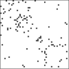
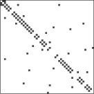
Figure 2: Simulated matrices over $d=50$ vertices. In panels (A) and (B), matrices with a block-diagonal structure and a small-world topology are respectively represented.

5.2 Noise Models

Resting-state or default-mode brain networks have been investigated by a large number of researchers in neuroimaging (Thirion et al., 2006; Beckmann et al., 2005). The main difficulty in simulating these networks stems from the absence of a prior to produce such resting-state patterns of activities (Leon et al., 2013; Kang et al., 2012). For each subject, we here constructed a set of $d$ sequences of $T$ realizations, where $d$ represents the number of ROIs, and $T$ denotes the total number of time points. These sequences of realizations were drawn from a multivariate Gaussian, such that for every subject, $i=1,\ldots,n$, the random vectors, $X_{itgm}\in\mathbb{R}^{d}$, were given by

$$X_{itgm}\stackrel{{\scriptstyle\operatorname{iid}}}{{\sim}}N_{d}(0,S_{gm}),\qquad\forall\;t=1,\ldots,T;$$

where $g=1,2$ denotes group affiliation, and $m=1,2$ denotes the choice of underlying adjacency matrix: block-diagonal model and small-world model.

Figure 3: Power curves for the simulated two-sample tests using the covariance estimation procedure, under a multivariate Gaussian model, with error bars based on one standard error from the mean. The $y$-axis indicates the probability of rejecting the null hypothesis when it is false; whereas the $x$-axis is a proxy measure of effect size (see Section 5.3). These results are presented for networks on $d=10,20,30$ and $40$ vertices, with different sample sizes and over $T=50$ time points, and based on $100$ iterations per condition with respect to the block (top row) and small-world (bottom row) topologies. A horizontal line has been added to indicate a power of $0.05$.

5.3 Simulation Results

Four main factors were made to vary in this set of simulations. In line with the subsequent real-data analysis, we considered sample sizes of $n=100,200,300$ and $400$ per group. This was deemed representative of the number of subjects found in most neuroimaging studies. Secondly, we varied network sizes, with $d$ taking values $10,20,30$, and $40$. This range of network sizes allowed us to identify the effect of network size on the statistical power of our test. Larger dimensions were expected to decrease power.

In each of these scenarios, we computed the statistical power of the two-sample tests, using different effect sizes. Here, the effect size was defined with respect to the value of the parameter $\eta$. Recall that $\eta$ controlled the distance between the two population means, such that $S_{2m}:=C(\eta-1)S_{1m}$. For each set of conditions, the simulations were repeated 100 times in order to obtain an empirical estimate of the theoretical power of the two-sample test statistic for Laplacians, under these conditions.

The results of these simulations are reported in Figure 3. The power of the two-sample test for Laplacians was found to be empirically well-behaved, for all the scenarios considered. In particular, this was true for both the block-diagonal and small-world topologies, as illustrated in the first and second row in Figure 3. As expected, the power of the test tended to increase with larger sample sizes, albeit that increase was mitigated by the size of the underlying networks.

6 Analysis of the 1000 FCP Data Set

Different aspects of the 1000 FCP data set were considered. Firstly, we used a one-sample test for comparing the Laplacian mean to a subsample of the data. We then tested for sex and age differences using the two- and $k$-sample tests for Laplacians. Finally, we analyzed differences in subnetworks, including the default-mode network (DMN). After excluding subjects for which demographics data were incomplete, we obtained a sample size of $n=1017$.

6.1 Inference on Full Data Set

As described in Section 1.2, the 1000 FCP data provides a unique opportunity for neuroscientists to extract a reference template of human connectivity. We tested the reliability of that template using a one-sample Laplacian test for some random subsample of the data. We computed the reference mean Laplacian over the full FCP sample, which is here treated as a population parameter, $\Lambda_{0}$. This was compared with a large random subsample of $917$ subjects –that is, after removing 100 subjects from the original FCP data. We then tested for the null hypothesis that the sample mean, $\widehat{L}_{1}$, was equal to the reference mean $\Lambda_{0}$. As expected, the test failed to reject the null hypothesis $(T_{1}=926,\text{df}=\binom{50}{2},p\approx 1)$, since the sample and reference means were drawn from the same population.

The partitioning of the 1000 FCP data set by sex is provided in Figure 1(A). This consists of $n_{f}=555$ female and $n_{m}=462$ male subjects. We tested whether such sex differences were significant using the two-sample test for Laplacians. The null hypothesis of no group differences was rejected with high probability ($T_{2}=1,689.5,\text{df}=\binom{50}{2},p<0.001$). These results should be compared with the use of a mass-univariate approach, in which a single hypothesis test is run for each voxel. The significant voxel-level differences detected using a mass-univariate approach for sex, is reported in Figure 4.

Subjects in the 1000 FCP database can also be grouped according to age. In Figure 1(B), we have divided the FCP sample into three subgroups of approximately equal sizes, with 386, 297, and 334 subjects; for subjects younger than 22, between 22 and 32, and older than 32, respectively. The $k$-sample Laplacian test (or Wilks’s Lambda) was performed to evaluate the hypothesis stating that these $k=3$ groups were drawn from the same population. The null hypothesis was also rejected with high probability in this case ($\Lambda=0.106,n=1,017,\text{df}=\binom{40}{2},p<0.001$). (For computational convenience, we here restricted our attention to networks with 40 nodes, which yielded invertible sample covariance matrices for the Wilks’s test.)

(A) Mass-univariate analysis                       (B) Multivariate analysis
   Uncorrected             Corrected             $\geq 85^{\text{th}}$ Percentile      $\geq 95^{\text{th}}$ Percentile
               

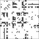
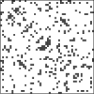
Figure 4: Comparison of edgewise differences using either a standard mass-univariate analysis, or our proposed multivariate method. In panel (A), mass-univariate analyses were conducted to test for local differences in connectivity due to sex in the full FCP data set ($n=1,017$). In each case, $\binom{50}{2}$ tests were performed independently for each of the off-diagonal entries in the Laplacians. The first matrix denotes the entries that were found to be significantly different between the groups at $\alpha=.05$; whereas the second matrix represents the significant entries after Bonferroni correction. Black denotes significant entries. In panel (B), the same edgewise effects are reported for our multivariate approach, using the visualization method described in Section 4.4. The edges whose contribution to the $T_{2}$-statistic is greater than the $85^{\text{th}}$ and $95^{\text{th}}$ percentiles (of the distribution of such individual contributions) have been plotted in black in the third and fourth panels, respectively.

6.2 Inference on Partial Data Set

The results of the previous section were compared with another analysis based on a small subset of connectomes. The 1000 FCP data set is indeed exceptionally large for the field of neuroimaging. By contrast, most papers using MRI data tend to report results based on smaller data sets, commonly containing between 20 and 100 subjects. Here, we have replicated the various statistical tests described in the last section for such small sample sizes, in order to produce an analysis more reflective of what might be performed by, say, a single lab.

The conclusions of the network-level tests for the different hypotheses of interest were found to be robust to a large decrease in sample size. As for the full data set, sex differences remain close to significance ($T_{2}=836.76,\text{df}=\binom{40}{2},p=0.077$), when solely considering 100 female and 100 male subjects. Note, however, that our proposed global test failed to reject the null hypothesis when considering smaller data sets. Indeed, we restricted our attention to smaller subsets of subjects, composed of 20 cases in each group, and such a test did not reject the null hypothesis ($T_{2}=514.96,\text{df}=\binom{40}{2},p\approx 1$).

These results should be contrasted with the use of a mass-univariate approach. We compared the conclusions of a network-level Laplacian test for sex, with the ones of a mass-univariate approach based on 100 female and 100 male subjects. No local differences were here found, after correcting for multiple comparisons, and solely one edge out of $\binom{40}{2}$ was found to significantly differ between groups at a threshold of $0.001$. This highlights one of the important advantages of using a global test in this context. While the mass-univariate approach fails to detect any sex differences at the local level, our proposed global test, by contrast, had sufficient power to reject the null hypothesis at a global level.

(A) Sex (DMN)                                  (B) Age (DMN)
       Female           Male                       $x\leq 22$        $22<x\leq 32$       $32<x$
                                  

Figure 5: Descriptive statistics for Default-Mode Network (DMN) in the 1000 FCP data set. In panels (A) and (B), we have provided the mean Laplacians after dividing the sample according to sex and age, respectively. As before, the Laplacians have been binarized with respect to the $75^{\text{th}}$ percentile in the distribution of the FCP database.

6.3 Default-Mode Network

The Default-Mode Network (DMN) is a widely studied portion of the functional network characterizing brain activity in both humans and animals (Greicius et al., 2003; Buckner, Andrews-Hanna and Schacter, 2008). This network tends to be active, when an individual is not engaged in a cognitive task. The DMN is composed of a set of hubs that include the precuneus, posterior cingulate, medial prefrontal cortex, and angular gyri, as well as prefrontal cortices, temporo-parietal junctions, the hippocampi, and the parahippocampi. In the parcellation template used in this paper, these regions corresponded to $d=24$ AAL areas.

We tested for the effect of sex in the full FCP sample by applying the projection method described in Equation (3). The hypothesis of no difference between males and females was not rejected for the DMN network ($T_{2}=1,128,\text{df}=\binom{24}{2},p\approx 1$). (The mean Laplacians for these subnetworks are reported in Figure 5.) This demonstrates that such multivariate methods also tends to lose power, when restricted to subnetworks.

7 Discussion

In this paper, we have analyzed a large neuroimaging data set, using a novel framework for network-based statistical testing. The development of this framework is grounded in a formal asymptotic theory for network averages, developed within the context of a well-defined notion of the space of graph Laplacians. Importantly, we have showed that using the global tests that result from our framework may provide the researcher with decidedly more statistical power than when using a mass-univariate approach, which is the standard approach in the field.

To the best of our knowledge, we are the first to ascribe a notion of a ‘space’ to the collection of graph Laplacians and to describe the geometrical properties of this space. While we have found it convenient for the purposes of exposition simply to summarize these results in the main body of the paper, and to collect details in the appendices, it is important to note that this initial step is crucial in allowing us to bring to bear recent probabilistic developments in the field of shape analysis to produce our key central limit theorem, upon which the distribution theory for our tests lies. We note too that the framework we offer is quite general and should, therefore, as a result be quite broadly applicable. Nevertheless, this initial work also has various limitations, and furthermore sets the stage for numerous directions for extensions, which we describe briefly below.

7.1 Limitations

It can be expected that there be a tradeoff in the performance of our tests between sample size $n$ and the dimension $d$ of the networks in the sample. This expectation is confirmed in our simulations, where one can observe that for a given sample size $n$, the rate of type I error increases beyond the nominal rate, as $d$ increases. Since our test can be seen to be equivalent to a Hotelling $T^{2}$ on the off-diagonal elements of the Laplacians, it follows that sample sizes of order $O(d^{2})$ would be required to control for this increase in type I error rate. For the analysis of the full FCP data set, this condition was approximately satisfied, since this data set contains more than 1000 subjects, and we were here comparing networks with $50$ vertices. In their current forms, such global statistical tests may therefore be most applicable to very large data sets, or to relatively small networks. However, our analysis of the smaller subsets of the FCP data (i.e., mimicking analysis at the level of a single lab) suggests that even at low sample sizes the test is well-powered against the alternative of differences in network group averages.

Computationally, the method employed in this paper was also challenging since the application of the Laplacian test required the inversion of a large covariance matrix. We have here resorted to different methods to facilitate this process including the use of modern shrinkage estimation techniques (Schäfer and Strimmer, 2005), as well as the modification of the resulting sample covariance matrix estimates in order to force positive definiteness (Cheng and Higham, 1998; Higham, 2002). Practically, however, such methods remain computational expensive, and may therefore limit the size of the networks that one may wish to consider when using such Laplacian tests.

Finally, observe that the networks of interest in this paper have been constructed using fMRI data. This preliminary step necessitated the estimation of covariance matrices for each subject, and such estimation has not been directly taken into account in the final analysis. Further research may therefore need to adopt a global modelling strategy in which the uncertainty at the first level of the analysis is propagated to the second level, in which we compare groups of subject-specific networks.

7.2 Extensions

In our work here (specifically, as described in Section 3) we show that the ‘space’ of networks – without any structural constraints – behaves ‘nicely’ from the mathematical perspective, and therefore we are able to develop a corresponding probability theory and statistical methods for one- and two-sample assessment of network data objects. However, one of the most fundamental results that has emerged from the past 20 years of complex network research is the understanding that real-world networks typically (although not exclusively) in fact tend to possess a handful of quite marked structural characteristics. For example, most networks are relatively sparse, in the sense that the number of edges is on the same order of magnitude as the number of vertices. Other common key properties include heterogeneous degree distributions, cohesive subgraphs (a.k.a. communities), and small-world behavior (see Newman, 2010, chap.8).

The ubiquity of such characteristics in real-world networks has been well-established. Importantly, this fact suggests that the appropriate (differential or metric measure) geometry of the ‘space of all networks’ – or, more formally, the space of Laplacians corresponding to such networks – depends both on the constraints imposed on these networks/Laplacians and the geometry chosen for the larger space ${\mathcal{P}}$ of PSD matrices. In our case, it is natural to choose a Euclidean geometry rather than geometries associated to ${\mathcal{P}}$ as a homogeneous space. In particular, other choices of network constraints can lead to metric geometry problems embedded inside Riemannian geometry problems. For examples, imposing sparseness on a network, or allowing for directed edges lead to nontrivial geometries. The Euclidean average of two sparse networks/matrices need not be sparse, and apart from simple scalings, one expects the set $\mathcal{L}$ of sparse matrices, properly defined, to be a discrete subset of the manifold of positive semi-definite matrices (PSD) and hence far from convex. Thus, it is natural to define the average of two sparse matrices to be the sparse matrix closest to the Euclidean average, but this may be computationally unappealing. Moreover, the Riemannian measure on PSD does not determine a measure on $\mathcal{L}$, so computing Fréchet means becomes problematic. Of course, one can impose a uniform distribution on $\mathcal{L}$, but this risks losing all geometric relations between $\mathcal{L}$ and PSD. Hence, there are a variety of open problems to be studied examining the implications of network structural constraints on the space $\mathcal{L}$.

Furthermore, since the asymptotic theory we exploit from shape analysis relies heavily on the topological and geometrical properties of the space within which they are brought to bear, we can expect that different network constraints will require different levels of effort in producing central limit theorems. More precisely, while a general asymptotic distribution theory for Fréchet means in metric spaces has recently been derived by Bhattacharya and Lin (2016), this theory requires that a number of conditions be satisfied, the verification of which can be expected to become increasingly difficult as the geometry of the space becomes complicated. Thus, accompanying the various extensions in geometry described above are likely to be corresponding challenges in probability theory and shape analysis. Some progress in this direction have been spearheaded by Bhattacharya et al. (2011) and Hotz et al. (2013), who have considered stratified spaces, and sticky CLTs for open books, respectively. Moreover, similar data object analyses have been conducted using phylogenetic trees (Skwerer et al., 2013). In object data analysis, the approach adopted in this paper would be regarded as extrinsic, in the sense that it embeds the manifold of interest in an ambient space. Further research may also investigate intrinsic approaches to study the set of graph Laplacians.

Finally, while the 1000 FCP data set is unique in its magnitude and richness, which in turn has allowed us to pose and answer a good number of questions relevant to neuroscience in the analyses using our proposed testing framework, there remains much additional empirical work to be done applying our methods, in order to more fully establish both their capabilities and their limitations. We would anticipate that with the recently started BRAIN initiative, and other endeavors like it, that within five years there will be a plethora of databases of network-based objects in neuroscience, providing more than ample motivation not only for the further testing of methods like the ones we have proposed here, but also for extending other tools from classical statistics to network data.

8 Supplementary Material

We here provide detailed proofs of the main results in this paper.

Proof of Theorem 1. Let the matrix $E$ of order $d\times d$ be partitioned in the following manner,

$$d-1\ \ 1\ \ \ \ \ \ \ \ \$$

$$E=\left(\begin{array}[]{cc}A&v\\ v^{\prime}&x\end{array}\right)\ \ \ \begin{array}[]{c}d-1\\ 1\end{array}$$

This matrix is assumed to satisfy conditions (1), (2), and (4). We will call the set of such matrices $\mathcal{T}.$ Assume that $A$, the top left $(d-1)\times(d-1)$ block of $E$, has nonzero determinant. We want to show that some $d(d-1)/2$-dimensional ball around $E$ continues to lie in $\mathcal{T}$. Since the rank of $E$ is $d-1$, the last column of $E$ is a linear combination of the first $d-1$ columns. Since the columns of $E$ add to zero and $E$ is symmetric, the rows of $E$ add to zero. For $v^{\prime}=(v_{1},\ldots,v_{d-1}),$ we must have

$$v_{i}=-\sum_{j=1}^{d-1}A_{ij},\qquad\text{and}\qquad x=-\sum_{j=1}^{d-1}v_{j}.$$

Thus, $v$ and $x$ are determined by the entries of $A$.

The matrix, $A$, is symmetric. Thus, it lies in the subspace $S$ of $\mathbb{R}^{(d-1)^{2}}$ of dimension $d(d-1)/2$ consisting of symmetric matrices. ${\rm Det}(A)\neq 0$, so for some matrix $A_{\epsilon}$ in some small neighborhood $U$ of $A$ in $S$, ${\rm det}(A_{\epsilon})\neq 0.$ Each choice of $A_{\epsilon}$ determines a corresponding $v$ and $x$. Conversely, each $E_{\epsilon}\in\mathcal{T}$ sufficiently close to $E$ in the $\mathbb{R}^{d^{2}}$ norm has $\det(A_{\epsilon})\neq 0$ and $A_{\epsilon}-A=X$ is symmetric, so $A_{\epsilon}$ and hence $E_{\epsilon}$ is determined by $X$. Thus, a neighborhood of $E$ in $\mathcal{T}$ is bijective to $U$. It is easy to check that this bijection is a diffeomorphism.

If some other $(d-1)\times(d-1)$ block $B$ of $E$ has nonzero determinant, we note that the top $(d-1)\times(d-1)$ block $A$ of the matrix determines the entire matrix as above. Any small symmetric perturbation $A_{\epsilon}$ of $A$ (with the necessary perturbations of the last row and column to preserve (4)) still satisfies $\det(B_{\epsilon})\neq 0$. Conversely, any $B\in\mathcal{T}$ sufficiently close to $E$ so that $\det(B_{\epsilon})\neq 0$ determines a symmetric perturbation of $A$ as above. Hence, we again obtain a neighborhood of $E$ in $\mathcal{T}$ parametrized by a neighborhood $U$ of $A$ in $S$. This shows that $\mathcal{T}$ is a submanifold of $\mathbb{R}^{d^{2}}$ of dimension $d(d-1)/2.$ The set of matrices satisfying (5) alone is an open convex cone in $\mathbb{R}^{d^{2}}$. When we intersect the submanifold $\mathcal{T}$ with this cone, we get an open submanifold $\mathcal{T}^{\prime}$ of $\mathcal{T}$. Thus $\mathcal{T}^{\prime}$, the set of matrices with (1), (2), (4), (5), is also a submanifold of $\mathbb{R}^{d^{2}}$ of dimension $d(d-1)/2.$

The space $\mathcal{T}^{\prime}$ has several connected components. A matrix $E_{0}$ with $k$ positive eigenvalues and a matrix $E_{1}$ with $k^{\prime}\neq k$ positive eigenvalues lie in different components, as a path in $\mathcal{T}^{\prime}$ from $E_{0}$ to $E_{1}$ would contain a matrix with a zero eigenspace of multiplicity at least two. Conversely, if $k=k^{\prime}$, then $E_{0}$ and $E_{1}$ are in the same component of $\mathcal{T}^{\prime}$. For the line segment $E_{t}=(1-t)E_{0}+tE_{1}$ stays in $\mathcal{T}^{\prime}$, for every $t\in[0,1]$. Since the components are open, the component of $\mathcal{T}^{\prime}$ satisfying $k=d-1$ is again a submanifold of dimension $d(d-1)/2.$ But this component has condition (3), and so is precisely $\mathcal{L}_{d}.$ This proves that $\mathcal{L}_{d}$ is a manifold of dimension $d(d-1)/2$.

For the convexity statement, conditions (2) – (5) are convex conditions; e.g. for (3), if $A$ and $B$ are positive semidefinite, then

$$\langle(tA+(1-t)B)v,v\rangle=t\langle Av,v\rangle+(1-t)\langle Bv,v\rangle\geq 0$$

for $t\in[0,1]$ and $v\neq 0$. Clearly, (1) – (5) together is a convex condition. For if $A$ and $B$ satisfy (1) – (5), then $A$ and $B$ come from weighted connected graphs, as does $tA+(1-t)B.$ Since a graph is connected iff the rank of the corresponding Laplacian matrix has rank $d-1$, the rank of $tA+(1-t)B$ is $d-1$ for $t\in[0,1].$ Thus $\mathcal{L}_{d}$ is a convex submanifold of $\mathbb{R}^{d^{2}}.$

To show that $\mathcal{L}_{d}$ lies in an affine subset, fix $E\in\mathcal{L}_{d}.$ For $k=d(d-1)/2$, take $k$ distinct points $s_{i}$ in $\mathcal{L}_{d}$, none of them equal to $E$, such that the convex hull of these points contains $E$. (For example, two of the points can be close to $E\pm S$ for a small symmetric matrix $S$.) For generic choices, the $k$ points plus $E$ determine an (affine) $k$-plane $P$, and the convex hull of these points lies in both $P$ and $\mathcal{S}$. Since $P$ and $\mathcal{L}_{d}$ have the same dimension, the open convex hull is exactly a neighborhood of $E$ in $\mathcal{L}_{d}$.

We now show that the plane $P$ is independent of the choice of $E.$ Since $\mathcal{L}_{d}$ is convex, it is connected. Take $F\in\mathcal{S}$, let $\ell$ be the Euclidean line segment from $E$ to $F$, and set $E_{t}=(1-t)E+tF\in\mathcal{L}_{d}.$ Arguing as above, we find a plane $P_{t}$ containing a neighborhood $V_{t}$ of $E_{t}$ in $\mathcal{L}_{d}.$ By compactness, there exist $0=t_{0},\ldots,t_{n}=1$ with $\cup_{i=0}^{n}V_{t_{i}}\supset\ell.$ If $P=P_{0}\neq P_{t_{1}}$, then some line segment from one of the $s_{i}$’s determining $P_{0}$ to one of the $s_{j}$’s determining $P_{t_{1}}$ does not lie in $\mathcal{L}_{d}$, a contradiction. Thus $P=P_{t_{1}}$, and by induction, $P=P_{1}.$ Since $F$ is arbitrary in $\mathcal{L}_{d}$, it follows that $\mathcal{L}_{d}$ lies in $P$. $\Box$

Proof of Corollary 1. In the notation of the proof of Theorem 1, assume that $E$ has conditions (1), (2), (4), (5^′). Then $A$ is symmetric and has $a_{ij}\leq 0.$ Thus $A$ is in bijection with the closed “quadrant” $\{(x^{1},\ldots,x^{d(d-1)/2}):x^{i}\leq 0\}$, which is the basic example of a manifold with corners. If the rank $d-1$ submatrix $B$ of $E$ is not in the top left corner, a relabeling of coordinates moves $B$ to the top left corner. Since the relabeling takes the closed quadrant to a closed quadrant, a neighborhood of $B$ has the structure of a manifold with corners. It is trivial to check that transition maps from chart to chart are smooth. If we impose (3), then as in the previous proof we pick out one connected component of this manifold with corners, and each component is a manifold with corners. The statements on convexity and affine subspaces follow immediately from Theorem 1, since $\mathcal{L}^{\prime}_{d}$ is a dense subset of $\mathcal{L}_{d}$. $\Box$

Proof of Theorem 2. Assume the $\ell\times\ell$ block with nonzero determinant occurs in the top left corner; the other cases are handled as in the proof of Theorem 1. Thus let

$$\ell\ \ \ \ \ \ \ d-\ell\ \ \ \ \ \ \ \ \$$

$$E=\left(\begin{array}[]{c|ccc}A&v_{1}&\ldots&v_{d-\ell}\\ \hline\cr v_{1}^{\prime}&&&\\ \vdots&b_{1}&\ldots&b_{d-\ell}\\ v_{d-\ell}^{\prime}&&&\end{array}\right)\ \ \ \begin{array}[]{ccccc}\ell\\ \\ d-\ell\\ \\ \end{array}$$

have conditions (1_ℓ), (2), (4). Here, $v_{i}$ is an $\ell\times 1$ column vector, and $b_{i}$ is a $(d-\ell)\times 1$ column vector. The dimension of the set of $\ell\times\ell$ symmetric matrices $A$ with nonzero determinant is $\ell(\ell+1)/2.$ Since the last $d-\ell$ columns must be linear combinations of the first $\ell$ columns, we have

$$v_{i}=\sum_{j=1}^{\ell}v_{ij}a_{j},\qquad i\in\{1,\ldots,d-\ell\};$$

where $a_{j}$ is the j^th column of $A$. The $v_{ij}$’s are arbitrary for $i=1,\ldots,d-\ell-1,$ but (4) implies that the $v_{d-\ell,j}$’s are determined by the previous $v_{ij}$’s. Therefore, we get another $(d-\ell-1)\ell$ degrees of freedom (i.e. dimensions), so the dimension of the space of matrices with (1_ℓ), (2), (4) is $\ell(\ell+1)/2+(d-\ell-1)\ell=d\ell-\ell(\ell+1)/2$. The argument for adding in conditions (3) and (5) goes as before. $\Box$

Proof of Theorem 3. The Laplacian CLT considered in this paper is a specialization of a general result due to Bhattacharya and Lin (2016), which considers a metric space $(\mathcal{X},\rho)$ equipped with a probability measure $Q$. In addition to the conditions stated in the main body of the paper, two further regularity assumptions must be made on the first and second derivatives of the function $\rho^{2}(\phi^{-1}(u),x)$. These conditions are described below as (A5) and (A6).

Bhattacharya and Lin (2016) have shown that Euclidean coordinates of a Fréchet mean defined on a metric space converges to a normal distribution, under the following assumptions: (A1) the Fréchet mean $\mu$, as described in equation (1) is unique; (A2) $\mu\in A\subseteq\mathcal{X}$, where $A$ is $Q$-measurable, and $\widehat{\mu}_{n}\in A$, almost surely; (A3) there exists a homeomorphism $\phi:A\to U$, for some $s\geq 1$, where $U$ is an open subset of $\mathbb{R}^{s}$; (A4) for every $u\in U$, the map, $u\mapsto h(u;x):=\rho^{2}(\phi^{-1}(u),x)$, is twice differentiable on $U$, for every $x\in\mathcal{X}$ outside a $Q$-null set; (A5) for every pair $1\leq k,l\leq s$, with $u\in U\subseteq\mathbb{R}^{s}$ and $x\in\mathcal{X}$, letting

$$D_{k}h(u;x):=\frac{\partial}{\partial u_{k}}h(u;x),\qquad\text{and}\qquad D_{k,l}h(u;x):=\frac{\partial^{2}}{\partial u_{k}\partial u_{l}}h(u;x),$$

we require that $\mathbb{E}\left[|D_{k}h(u;x)|^{2}\right]<\infty$, and $\mathbb{E}\left[|D_{k,l}h(u;x)|\right]<\infty$; moreover, (A6) defining $f_{k,l}(\epsilon,x):=\sup\{|D_{k,l}h(u;x)-D_{k,l}h(\phi(\mu);x)|:|u-\phi(\mu)|<\epsilon\}$, we also require modulus continuity, such that $\mathbb{E}[|f_{k,l}(\epsilon;Y)|]\to 0$, as $\epsilon\to 0$, for every $1\leq k,l\leq s$; and finally, (A7) the matrix, $B:=\{\mathbb{E}[D_{k,l}h(\phi(\mu);Y)]\}_{k,l=1,\ldots,s}$, should be non-singular. Under these conditions, it is then true that the following convergence in distribution holds,

$$n^{1/2}\left(\phi(\widehat{\mu}_{n})-\phi(\mu)\right)\longrightarrow N(0,B^{-1}VB^{-T}),$$

where $V:=\operatorname{\mathbb{C}ov}[D\,h(\phi(\mu);Y)]$ is assumed to be non-singular.

In our setting, we have drawn an iid sample of combinatorial Laplacians from an unknown generating distribution, such that we have $Y_{i}\sim F(\Lambda,\Sigma)$, for every $i=1,\ldots,n$, where $\Lambda$ and $\Sigma$ are the mean Laplacian and the covariance matrix of the upper triangle of $Y$, with respect to some unknown distribution, $F$. Observe that the space of interest is here $\mathcal{L}^{\prime}_{d}$, equipped with the Frobenius distance, as stated in Corollary 1, thereby forming the metric space, $(\mathcal{L}^{\prime}_{d},\|\cdot\|_{F})$. We will see that conditions (A1) – (A4) as well as (A7) are necessarily satisfied in our context. Moreover, we will assume that conditions (A5) and (A6) also hold.

Condition (A1) is readily satisfied, since we have demonstrated that the space of interest, $\mathcal{L}^{\prime}_{d}$, is a convex subspace of $\mathbb{R}^{d^{2}}$; and moreover the arithmetic mean is a convex function on that space by Corollary 1. Thus, the sample Fréchet mean, $\widehat{L}_{n}$, is unique, for every $n\in\mathbb{N}$. Secondly, we have assumed that the underlying measure gives a non-zero positive probability to a subset $U\in\mathbb{R}^{d^{2}}$, which contains $\Lambda$. Therefore, condition (A2) is satisfied, in the sense, that there exists a subset $A\subseteq\mathbb{M}_{d,d}(\mathbb{R}^{+})$, such that $A$ is $\mathbb{P}$-measurable. In addition, since the strong law of large numbers holds for the Fréchet mean (see Ziezold, 1977), we also know that $\widehat{L}_{n}\to\Lambda$, almost surely; and therefore, $\mathbb{P}[\widehat{L}_{n}\in A]\to 1$, as $n\to\infty$, as required by condition (A2).

For condition (A3), observe that, in our context, the homeomorphism of interest, $\phi:A\mapsto U$, is the half-vectorization function. This takes a matrix in $\mathcal{L}^{\prime}_{d}$, and returns a vector in $\mathbb{R}^{\binom{d}{2}}$, such that for every $Y\in\mathcal{L}^{\prime}_{d}$, $\phi(Y):=\operatorname{vech}(Y)$. Specifically, this vectorization is defined by a change of indices, such that for every $i\leq j$, with $1\leq i,j\leq d$, we have $[\phi(Y)]_{k(i,j)}:=y_{ij}$, with $k(i,j):=(i-1)d+j$. The inverse function, $\phi^{-1}$, is then readily obtained for every $u\in U\subseteq\mathbb{R}^{\binom{d}{2}}$, satisfying $\phi^{-1}(u)=Y$, as $[\phi^{-1}(u)]_{ij}=y_{ij}$. The bicontinuity of $\phi$ is hence trivially verified and this map is therefore a homeomorphism.

For condition (A4), the function $h(u;Y):=\rho^{2}(\phi^{-1}(u),Y)$, for every $u\in U\subseteq\mathbb{R}^{\binom{d}{2}}$ and every $Y\in\mathcal{L}^{\prime}_{d}$, outside of a $Q$-null set, is here defined as

$$h(u;Y):=||\phi^{-1}(u)-Y||_{F}^{2}=\sum_{i\leq j}^{d}\,\Big{(}[\phi^{-1}(u)]_{ij}-y_{ij}\Big{)}^{2},$$

where the sum is taken over all the pairs of indices $1\leq i,j\leq d$, satisfying $i\leq j$. The first derivative of this map with respect to the coordinates of the elements of $\mathcal{L}^{\prime}_{d}$ in $\mathbb{R}^{\binom{d}{2}}$, is straightforwardly obtained. Setting $X:=\phi^{-1}(u)$, we have

$$D_{k(i,j)}h(u;Y):=\frac{\partial}{\partial u_{k(i,j)}}||\phi^{-1}(u)-Y||_{F}^{2}=2(x_{ij}-y_{ij}).$$

The second derivative of $h(u;Y)$ can be similarly derived for every quadruple, $1\leq i,j,i^{\prime},j^{\prime}\leq d$, satisfying $k(i,j)\neq k(i^{\prime},j^{\prime})$. When expressed with respect to $\Lambda\in U$, this gives

$$D_{k(i,j),k(i^{\prime},j^{\prime})}h(\phi(\Lambda);Y)=\begin{cases}2,&\text{if }k(i,j)=k(i^{\prime},j^{\prime}),\\ 0,&\text{otherwise}.\end{cases}$$

It immediately follows that the matrix of second derivatives is $B=2I$, and hence condition (A4) is verified. In addition, we have assumed that conditions (A5) and (A6) hold in our context. Finally, we have seen that the matrix $B$ is diagonal and hence non-singular, as required by condition (A7).

We can also compute the covariance matrix of the resulting multivariate normal distribution. For this, we require the matrix $V:=\operatorname{\mathbb{C}ov}[D\,h(\phi(\Lambda);Y)]$. Given our choice of $\phi$, we need to consider the mean vector of $D\,h(\phi(\Lambda);Y)$, which is given for every $1\leq i,j\leq n$ by $\mathbb{E}[D_{k(i,j)}\,h(\phi(\Lambda);Y)]=2(\Lambda_{ij}-\mathbb{E}[Y]_{ij})=0$. We can then compute the elements of $V$. For every quadruple $1\leq i,j,i^{\prime},j^{\prime}\leq n$, this gives

$$V_{k(i,j),k(i^{\prime},j^{\prime})} =\mathbb{E}[D_{k(i,j)}\,h(\phi(\Lambda);Y)\cdot D_{k(i^{\prime},j^{\prime})}\,h(\phi(\Lambda);Y)]$$

$$=4\mathbb{E}[(\Lambda_{ij}-Y_{ij})(\Lambda_{i^{\prime},j^{\prime}}-Y_{i^{\prime}j^{\prime}})]$$

$$=4\big{(}\mathbb{E}[Y_{ij}Y_{i^{\prime}j^{\prime}}]-\Lambda_{ij}\Lambda_{i^{\prime},j^{\prime}}\big{)},$$

since the cross-term vanishes, after taking the expectation. Therefore, the asymptotic covariance matrix in Theorem 3 is indeed equal to the covariance matrix of the distribution, from which the $Y_{i}$’s have been sampled. That is, this covariance matrix is given by $B^{-1}VB^{-T}=(2I)^{-1}V(2I)^{-1}=\operatorname{\mathbb{V}ar}[\phi(Y)]=\Sigma$. Therefore, all the conditions of Theorem 2.1 of Bhattacharya and Lin (2016) have been satisfied, and hence $n^{1/2}(\phi(\widehat{L}_{n})-\phi(\Lambda))\to N(0,\Sigma)$, as stated in Theorem 3.

References

- Achard et al. (2006) {barticle}[author] \bauthor\bsnmAchard, \bfnmSophie\binitsS., \bauthor\bsnmSalvador, \bfnmRaymond\binitsR., \bauthor\bsnmWhitcher, \bfnmBrandon\binitsB., \bauthor\bsnmSuckling, \bfnmJohn\binitsJ. and \bauthor\bsnmBullmore, \bfnmEd\binitsE. (\byear2006). \btitleA Resilient, Low-Frequency, Small-World Human Brain Functional Network with Highly Connected Association Cortical Hubs. \bjournalJ. Neurosci. \bvolume26 \bpages63–72. \endbibitem
- Anderson (2003) {bbook}[author] \bauthor\bsnmAnderson, \bfnmT. W.\binitsT. W. (\byear2003). \btitleAn Introduction to Multivariate Statistical Analysis (Third edition). \bpublisherWiley, \baddressWiley. \endbibitem
- Arsigny et al. (2007) {barticle}[author] \bauthor\bsnmArsigny, \bfnmV.\binitsV., \bauthor\bsnmFillard, \bfnmP.\binitsP., \bauthor\bsnmPennec, \bfnmX.\binitsX. and \bauthor\bsnmAyache, \bfnmN.\binitsN. (\byear2007). \btitleGeometric means in a novel vector space structure on symmetric positive-definite matrices. \bjournalSIAM Journal on Matrix Analysis and Applications \bvolume29 \bpages328–347. \endbibitem
- Aydin et al. (2009) {barticle}[author] \bauthor\bsnmAydin, \bfnmBurcu\binitsB., \bauthor\bsnmPataki, \bfnmGábor\binitsG., \bauthor\bsnmWang, \bfnmHaonan\binitsH., \bauthor\bsnmBullitt, \bfnmElizabeth\binitsE. and \bauthor\bsnmMarron, \bfnmJS\binitsJ. (\byear2009). \btitleA principal component analysis for trees. \bjournalThe Annals of Applied Statistics \bpages1597–1615. \endbibitem
- Barden, Le and Owen (2013) {barticle}[author] \bauthor\bsnmBarden, \bfnmDennis\binitsD., \bauthor\bsnmLe, \bfnmHuiling\binitsH. and \bauthor\bsnmOwen, \bfnmMegan\binitsM. (\byear2013). \btitleCentral limit theorems for Frechet means in the space of phylogenetic trees. \bjournalElectron. J. Probab \bvolume18 \bpages1–25. \endbibitem
- Beckmann et al. (2005) {barticle}[author] \bauthor\bsnmBeckmann, \bfnmChristian F\binitsC. F., \bauthor\bsnmDeLuca, \bfnmMarilena\binitsM., \bauthor\bsnmDevlin, \bfnmJoseph T\binitsJ. T. and \bauthor\bsnmSmith, \bfnmStephen M\binitsS. M. (\byear2005). \btitleInvestigations into resting-state connectivity using independent component analysis. \bjournalPhilosophical Transactions of the Royal Society B: Biological Sciences \bvolume360 \bpages1001–1013. \endbibitem
- Bhatia (1997) {bbook}[author] \bauthor\bsnmBhatia, \bfnmR.\binitsR. (\byear1997). \btitleMatrix Analysis. \bpublisherSpringer, \baddressNew York. \endbibitem
- Bhatia (2007) {bbook}[author] \bauthor\bsnmBhatia, \bfnmR.\binitsR. (\byear2007). \btitlePositive Definite Matrices. \bpublisherPrinceton University Press, \baddressPrinceton. \endbibitem
- Bhattacharya and Bhattacharya (2012) {bbook}[author] \bauthor\bsnmBhattacharya, \bfnmA.\binitsA. and \bauthor\bsnmBhattacharya, \bfnmR.\binitsR. (\byear2012). \btitleNonparametric Inference on Manifolds with Applications to Shape Spaces. \bpublisherCambridge University Press, \baddressNew York. \endbibitem