Privacy-Preserving Filtering for Event Streams

Abstract

Many large-scale information systems such as intelligent transportation systems, smart grids or smart buildings collect data about the activities of their users to optimize their operations. To encourage participation and adoption of these systems, it is becoming increasingly important that the design process take privacy issues into consideration. In a typical scenario, signals originate from many sensors capturing events involving the users, and several statistics of interest need to be continuously published in real-time. This paper considers the problem of providing differential privacy guarantees for such multi-input multi-output systems processing event streams. We show how to construct and optimize various extensions of the zero-forcing equalization mechanism, which we previously proposed for single-input single-output systems. Some of these extensions can take a model of the input signals into account. We illustrate our privacy-preserving filter design methodology through the problem of privately monitoring and forecasting occupancy in a building equipped with multiple motion detection sensors.

I Introduction

Privacy issues associated with social networking applications or monitoring and decision systems collecting personal data to operate are receiving an increasing amount of attention [3, 4]. Indeed, privacy concerns are already resulting in delays or cancellations in the deployment of some smart power grids, location-based services, or civilian unmanned aerial systems for example [5]. In order to encourage the adoption of these systems, which can provide important societal benefits, new tools are needed to provide clear privacy protection guarantees and allow users to balance utility with privacy rigorously [6].

Since offering privacy guarantees for a system generally involves sacrificing some level of performance, evaluating the resulting trade-offs requires a quantitative definition of privacy. Various such definitions have been proposed, such as disclosure risk [7] in statistics, $k$-anonymity [8], information-theoretic privacy [9], or conditions based on observability [10, 11]. However, in the last few years the notion of differential privacy has emerged essentially as a standard specification [12, 13]. Intuitively, a system processing privacy-sensitive inputs from individuals is differentially private if its published outputs are not too sensitive to the data provided by any single participant. This definition is naturally linked to the notion of system gain for dynamical systems, see [14, 15]. One operational advantage of differential privacy compared to other definitions is that it provides strong guarantees without involving the difficult task of modeling all the available auxiliary information that could be linked to the published outputs, despite the fact that unanticipated privacy breaches are typically due to the presence of this side information [8, 16, 17].

Differential privacy is a strong notion of privacy, but might require large perturbations to the published results of an analysis in order to hide individuals’ data. This is especially true for applications where users continuously contribute data over time, and it is thus important to carefully design real-time mechanisms that can limit the impact on system performance of differential privacy requirements. Previous work on designing differentially private mechanisms for the publication of time series include [18, 19], but these mechanisms are not causal and hence not suited for real-time applications. The ZFE mechanism of Section IV could also be interpreted as a dynamic, causal version of the matrix mechanism introduced in [20] for static databases. The papers [21, 22, 23] describe real-time differentially private mechanisms to approximate a few specific filters processing a stream of $0-1$ variables, representing the occurence of events attributed to individuals. For example, [21, 22] consider a private accumulator providing at each time the total number of events that occurred in the past. This paper is inspired by this scenario, and builds on our previous work on this problem in [14, Section IV] [15, Section VI]. Here we extend our analysis in particular to multi-input multi-output (MIMO) linear time-invariant systems, which considerably broadens the applicability of the model to more common situations where multiple sensors monitor an environment and we wish to concurrently publish several statistics of interest. An application example is that of analyzing spatio-temporal records provided by networks of simple counting sensors, e.g., motion detectors in buildings or inductive-loop detectors in traffic information systems [24]. The literature on the differentially private processing of multi-dimensional time series is still very limited, but includes [25], which considers a single-input multiple-output filter where each output channel corresponds to a moving average filter with a different size for the averaging window, as well as [26], which discusses an application to traffic monitoring.

To summarize, the contributions and organization of this paper are as follows. In Section II, we present a new generic scenario where we need to approximate a general MIMO linear time-invariant system by a mechanism offering differential privacy guarantees for the input signals. The formal definitions necessary to state the problem are also provided in that section. In Section III we perform some preliminary system sensitivity calculations that are necessary in the rest of the paper. Section IV presents a general approximation scheme for MIMO systems that provides differential privacy guarantees for the input signals. The design methodology and performance of the privacy-preserving filter are illustrated in Section V in the context of a building occupancy estimation problem. Note that Sections III-V provide a more detailed presentation of the theoretical and simulation results contained in our conference paper [2]. Finally, Section VI presents additional privacy-preserving mechanisms that can approximate the desired outputs more closely but require more information about the input signals to be publicly available, .e.g., their second-order statistics. It improves and extends to the MIMO case the results presented in our conference paper [1]. This section also illustrates the relationship between our problem and certain joint Transmitter-Receiver optimization problems arising in the communication systems literature [27, 28].

Notation: Throughout the paper we use the following standard abbreviations: LTI for Linear Time-Invariant, SISO for Single-Input Single-Output, SIMO for Single-Input Multiple-Output, and MIMO for Multiple-Input Multiple-Output. Unless specified otherwise, dynamical systems or filters are assumed causal, and transfer functions have real-valued coefficients. We fix a base probability space $(\Omega,\mathcal{F},\mathbb{P})$. For $m$ an integer with $m\geq 1$, we write $[m]:=\{1,\ldots,m\}$. The notations $|x|_{1}=\sum_{k=1}^{p}|x_{k}|$ and $|x|_{2}=\left(\sum_{k=1}^{p}|x_{k}|^{2}\right)^{1/2}$ are used to denote the $1$- and $2$-norms in $\mathbb{R}^{p}$ or $\mathbb{C}^{p}$, and we reserve the notation $\|\cdot\|$ for norms on signal and system spaces. $\text{col}(x_{1},\ldots x_{p})$ denotes a column vector or signal with components $x_{i}$, $i=1,\ldots,p$, and $\text{diag}(x_{1},\ldots,x_{m})$ denotes a diagonal $m\times m$ matrix with the $x_{i}$’s on the diagonal. Finally, for $H$ a Hermitian matrix, $H\succ 0$ means that it is positive definite, and $H\succeq 0$ that it is positive semi-definite.

II Problem Statement

II-A Generic Scenario

We consider $m$ sensors detecting events, with sensor $i$ producing a discrete-time scalar signal $\{u_{i,t}\}_{t\geq 0}\in\mathbb{R}$, for $i\in[m]$. In a building monitoring scenario for example, the sensors could be motion detectors distributed at various locations and polled at regular intervals, with $u_{i,t}\in\mathbb{N}$ the number of detected events reported for period $t$. We denote $u$ the resulting vector-valued signal, i.e., $u_{t}\in\mathbb{R}^{m}$. A linear time-invariant (LTI) filter $F$, with $m$ inputs and $p$ outputs, takes input signals $u$ from the sensors and publishes output signals $y=Fu$ of interest, with $y_{t}\in\mathbb{R}^{p}$. In our example, we might be interested in continuously updating real-time estimates of the number of people in various parts of the building, as well as short- and medium-term occupancy forecasts, in order to optimize the operations of the Heating, Ventilation, and Air Conditioning (HVAC) system. The problem considered in this paper consists in replacing the filter $F$ by a system processing the input $u$ and producing a signal $\hat{y}$ as close as possible to the desired output $y$ (minimizing for example the mean squared error $\lim_{T\to\infty}\frac{1}{T}\sum_{t=0}^{\infty}\mathbb{E}[|y_{t}-\hat{y}_{t}|_{2}^{2}]$), while providing some privacy guarantees to the individuals from which the input signals $u$ originate. The privacy constraint is explained and quantified in the next subsection.

II-B Differential Privacy

As mentioned in the introduction, a differentially private mechanism publishes data in a way that is not too sensitive to the presence or absence of a single individual. A formal definition of differential privacy is provided in Definition 1 below. In the previous building monitoring example, one goal of a privacy constraint could be to provide guarantees that an individual cannot be tracked too precisely from the published (typically aggregate) data. Indeed, Wilson and Atkeson [29] for example demonstrate how to track individual users in a building using a network of simple binary sensors such as motion detectors.

II-B1 Adjacency Relation

Formally, we start by defining a symmetric binary relation, denoted Adj, on the space $\mathsf{D}$ of datasets of interest, which captures what it means for two datasets to differ by the data of a single individual. Essentially, it is hard to determine from a differentially private output which of any two adjacent input datasets was used. Here, $\mathsf{D}:=\{u:\mathbb{N}\mapsto\mathbb{R}^{m}\}$ is the set of input signals, and we have $\text{Adj}(u,u^{\prime})$ if and only if we can obtain the signal $u^{\prime}$ from $u$ by adding or subtracting the events corresponding to just one user. Motivated again by applications to spatial monitoring, we consider in this paper the following adjacency relation

$$\text{Adj}(u,u^{\prime})\text{ iff }\forall i\in[m],\exists t_{i}\in\mathbb{N},\alpha_{i}\in\mathbb{R},\text{ s.t. }u^{\prime}_{i}-u_{i}=\alpha_{i}\delta_{t_{i}},|\alpha_{i}|\leq k_{i},$$ (1)

parametrized by a vector $k\in\mathbb{R}^{m}$ with components $k_{i}>0$. According to (1), a single individual can affect each input signal component at a single time (here $\delta_{t_{i}}$ denotes the discrete impulse signal with impulse at $t_{i}$), and by at most $k_{i}$. Let $e_{i}\in\mathbb{R}^{m}$ be the $i^{th}$ basis vector, i.e., with coordinates $e_{ij}=\delta_{ij},j=1,\ldots,m$. Then for two adjacent signals $u$, $u^{\prime}$, we have with the notation in (1)

$$u^{\prime}-u=\sum_{i=1}^{m}\alpha_{i}\delta_{t_{i}}e_{i}.$$ (2)

Note in passing that we can place additional constraints on $k$ to capture additional knowledge about the problem, which can help design mechanisms with better performance, as we discuss later. For example, if we known that a given person can activate at most $l<m$ sensor and each $k_{i}$ is $1$, we can add the constraint $|k|_{1}\leq l$.

The adjacency relation (1) extends the one considered in [21, 22, 15] to the case of multiple input signals. It puts two constraints on the influence that an individual can have on the input data in order for a differentially private mechanism to offer him guarantees. First, any given sensor can report an event due to the presence of the individual only once over the time interval of interest for our analysis. This is a sensible constraint in applications such as traffic monitoring with fixed motion detectors activated only once by each car traveling along a road, certain location-based services where a customer would check-in say at most once per day at each visited store, or certain health-monitoring applications where an individual would report a sickness only once. For a building monitoring scenario however, a single user could trigger the same motion detector several times over a relatively short period. A first solution consists in splitting the data stream of problematic sensors into several successive intervals, each considered as the signal from a new virtual sensor, so that an individual’s data is present only once in each interval. A MIMO mechanism can then process such data and offer guarantees, addressing one of the main issues for the applicability of the model proposed in [21, 22]. However, increasing the number of inputs degrades the privacy guarantees or the output quality that we can provide. Hence in general no privacy guarantee will be offered to users who activate the same sensor too frequently. The second constraint imposed by (1) is that we bound the magnitude of an individual’s contribution by $k_{i}$, but this is not really problematic in applications such as motion detection, where we can typically take $k_{i}=1$.

II-B2 Definition of Differential Privacy

Mechanisms that are differentially private necessarily randomize their outputs, in such a way that they satisfy the following property [12, 13, 30].

Definition 1.

Let $\mathsf{D}$ be a space equipped with a symmetric binary relation denoted Adj, and let $(\mathsf{R},\mathcal{M})$ be a measurable space. Let $\epsilon,\delta\geq 0$. A mechanism $M:\mathsf{D}\times\Omega\to\mathsf{R}$ is $(\epsilon,\delta)$-differentially private for Adj (and $\mathcal{M}$) if for all $d,d^{\prime}\in\mathsf{D}$ such that $\text{Adj}(d,d^{\prime})$, we have

$$\mathbb{P}(M(d)\in S)\leq e^{\epsilon}\mathbb{P}(M(d^{\prime})\in S)+\delta,\;\;\forall S\in\mathcal{M}.$$ (3)

If $\delta=0$, the mechanism is said to be $\epsilon$-differentially private.

This definition quantifies the allowed deviation for the output distribution of a differentially private mechanism for two adjacent datasets $d$ and $d^{\prime}$. One can also show that it is impossible to design a statistical test with small error to decide if $d$ or $d^{\prime}$ was used by a differentially private mechanism to produce its output [31, 32]. In this paper, the space $\mathsf{D}$ was defined as the space of input signals, and the adjacency relation considered is (1). The output space $\mathsf{R}$ is simply the space of output signals $\mathsf{R}:=\{y:\mathbb{N}\to\mathbb{R}^{p}\}$. Finally, a differentially private mechanism will consist of a system approximating our MIMO filter of interest $F$, as well as a source of noise necessary to randomize the outputs and satisfy (1). We also refer the reader to [14] for a technical discussion on the (standard) $\sigma$-algebra $\mathcal{M}$ used on the output signal space to offer useful guarantees.

II-B3 Sensitivity

Enforcing differential privacy can be done by randomly perturbing the published output of a system, at the price of reducing its utility or quality. Hence, we are interested in evaluating as precisely as possible the amount of noise necessary to make a mechanism differentially private. For this purpose, the following quantity plays an important role.

Definition 2.

The $\ell_{2}$-sensitivity of a system $G$ with $m$ inputs and $p$ outputs with respect to the adjacency relation Adj is defined by

$$\Delta^{m,p}_{2}G =\sup_{\text{Adj(u,u')}}\|Gu-Gu^{\prime}\|_{2}=\sup_{\text{Adj(u,u')}}\|G(u-u^{\prime})\|_{2},$$

where by definition $\|Gv\|_{2}=\sqrt{\sum_{t=-\infty}^{\infty}|(Gv)_{t}|_{2}^{2}}$.

II-B4 A Basic Differentially Private Mechanism

The basic mechanism of Theorem 1 below (see [15]), extending [30], can be used to answer queries in a differentially private way. To present the result, we recall first the definition of the $\mathcal{Q}$-function $\mathcal{Q}(x):=\frac{1}{\sqrt{2\pi}}\int_{x}^{\infty}e^{-\frac{u^{2}}{2}}du$. Now for $\epsilon,\delta>0$, let $K=\mathcal{Q}^{-1}(\delta)$ and define $\kappa_{\delta,\epsilon}=\frac{1}{2\epsilon}(K+\sqrt{K^{2}+2\epsilon})$.

Theorem 1.

Let $G$ be a system with $m$ inputs and $p$ outputs, and with $\ell_{2}$-sensitivity $\Delta^{m,p}_{2}G$ with respect to an adjacency relation Adj. Then the mechanism $M(u)=Gu+w$, where $w$ is a $p$-dimensional Gaussian white noise with covariance matrix $\kappa_{\delta,\epsilon}^{2}(\Delta^{m,p}_{2}G)^{2}I_{p}$ is $(\epsilon,\delta)$-differentially private with respect to Adj.

The mechanism $M$ described in Theorem 1, which is a differentially-private version of a system $G$, is called an output-perturbation mechanism. We see that the amount of noise sufficient for differential privacy with this mechanism is proportional to the $\ell_{2}$-sensitivity of the filter and to $\kappa_{\delta,\epsilon}$, which can be shown to behave roughly as $O(\ln(1/\delta))^{1/2}/\epsilon$. Note that we add noise proportional to the sensitivity of the whole filter $G$ independently on each output, even if $G$ was diagonal say, otherwise trivial attacks that simply average a sufficient number of outputs could potentially detect the presence of an individual with high probability [15].

In conclusion we could obtain a differentially private mechanism for our original problem by simply adding a sufficient amount of noise to the output of our desired filter $F$, provided we can compute its sensitivity, which is the topic of the next section. Moreover, it is possible in general to design mechanisms with much less overall noise than this output-perturbation scheme, as discussed in Sections IV and VI.

III Sensitivity Calculations

For the following sensitivity calculations (see Definition 2), the $\mathcal{H}_{2}$ norm of an LTI system plays an important role. We recall its definition for a system $G$ with $m$ inputs

$$\|G\|_{2}^{2}=\sum_{i=1}^{m}\|G\delta_{0}e_{i}\|_{2}^{2}=\frac{1}{2\pi}\int_{-\pi}^{\pi}\text{Tr}(G^{*}(e^{j\omega})G(e^{j\omega}))d\omega.$$

Writing $G(z)=[G_{ij}(z)]_{i,j}$ for the $p\times m$ transfer matrix, we also note from the frequency domain definition that $\|G\|_{2}^{2}=\sum_{i,j}\|G_{ij}\|_{2}^{2}.$

III-A Exact solutions for the SIMO and Diagonal Cases

Generalizing the SISO scenario considered in [14, 15] to the case of a SIMO system, we have immediately the following theorem.

Theorem 2 (SIMO LTI system).

Let $G$ be a stable LTI system with one input and $p$ outputs. For the adjacency relation (1), we have $\Delta^{1,p}_{2}G=k_{1}\|G\|_{2},$ where $\|G\|_{2}$ is the $\mathcal{H}_{2}$ norm of $G$.

Proof.

We have immediately for $u$ and $u^{\prime}$ adjacent

$$\|G(u-u^{\prime})\|^{2}_{2} =|\alpha_{1}|^{2}\|G\delta_{t_{1}}\|^{2}_{2}\leq k^{2}_{1}\|G\|^{2}_{2},$$

and the bound is attained if $|\alpha_{1}|=k_{1}$. ∎

For a system $G$ with multiple inputs, the special case where $G$ is diagonal, i.e., its transfer matrix is $G(z)=\text{diag}(G_{11}(z),\ldots,G_{mm}(z))$, also leads to a simple sensitivity result. Note that in this case, we have $\|G\|_{2}^{2}=\sum_{i=1}^{m}\|G_{ii}\|^{2}$.

Theorem 3 (Diagonal LTI system).

Let $G$ be a stable diagonal LTI system with $m$ inputs and outputs. For the adjacency relation (1), denoting $K=\text{diag}(k_{1},\ldots,k_{m})$, we have

$$\Delta^{m,m}_{2}G=\|GK\|_{2}=\left(\sum_{i=1}^{m}\|k_{i}G_{ii}\|_{2}^{2}\right)^{1/2}.$$

Proof.

If $G$ is diagonal, then for u and u’ adjacent, we have from (2)

$$\|G(u-u^{\prime})\|^{2}_{2} =\left\|\sum_{i=1}^{m}\alpha_{i}G\delta_{t_{i}}e_{i}\right\|^{2}_{2}=\|\text{col}(\alpha_{1}g_{11}*\delta_{t_{1}},\ldots,\alpha_{m}g_{mm}*\delta_{t_{m}})\|^{2}_{2},$$

where $g_{ii}$ denotes the impulse response of $G_{ii}$. Hence

$$\|G(u-u^{\prime})\|^{2}_{2} =\sum_{i=1}^{m}\|\alpha_{i}g_{ii}*\delta_{t_{i}}\|_{2}^{2}=\sum_{i=1}^{m}|\alpha_{i}|^{2}\|G_{ii}\|_{2}^{2},$$

and $|\alpha_{i}|\leq k_{i}$, for all $i$. Again the bound is attained if $|\alpha_{i}|=k_{i}$ for all $i$. ∎

III-B Upper and Lower Bound for the general MIMO Case

For MISO or general MIMO systems, the sensitivity calculations are no longer so straightforward, because the impulses on the various input channels, obtained from the difference of two adjacent signals $u,u^{\prime}$, all possibly influence any given output. Still, the following result provides simple bounds on the sensitivity.

Theorem 4.

Let $G$ be a stable LTI system with $m$ inputs and $p$ outputs. For the adjacency relation (1), denoting $K=\text{diag}(k_{1},\ldots,k_{m})$, and $|k|_{2}=\left(\sum_{i=1}^{m}k_{i}^{2}\right)^{1/2}$, we have

$$\|GK\|_{2}\leq\Delta^{m,p}_{2}G\leq|k|_{2}\|G\|_{2}.$$ (4)

Proof.

We have $G(u-u^{\prime})=\sum_{i=1}^{m}\alpha_{i}\,G\delta_{t_{i}}e_{i},$ and moreover $\|G\|^{2}_{2}=\sum_{i=1}^{m}\|G\delta_{t_{i}}e_{i}\|_{2}^{2}$ by definition. For the upper bound, we can write

$$\|G(u-u^{\prime})\|_{2} =\left\|\sum_{i=1}^{m}\alpha_{i}\,G\delta_{t_{i}}e_{i}\right\|_{2}$$

$$\leq\sum_{i=1}^{m}|\alpha_{i}|\|G\delta_{t_{i}}e_{i}\|_{2}$$

$$\leq|k|_{2}\left(\sum_{i=1}^{m}\|G\delta_{t_{i}}e_{i}\|^{2}_{2}\right)^{1/2},$$

where the last inequality results from the Cauchy-Schwarz inequality.

For the lower bound, let us first take $u^{\prime}\equiv 0$. Then consider an adjacent signal $u$ with a single discrete impulse of height $k_{i}$ at time $t_{i}$ on each input channel $i$, for $i=1,\ldots,m$, with $t_{1}<t_{2}<\ldots<t_{m}$. Let $\eta>0$. Denote the “columns” of $G$ as $G_{i}$ for $i=1,\ldots,m$, i.e., $Gu=\sum_{i=1}^{m}G_{i}u_{i}$. Since $\|G\|_{2}<\infty$, $\|G_{i}u_{i}\|_{2}<\infty$, and hence $|(G_{i}u_{i})_{t}|\to 0$ as $t\to\infty$. Hence by taking $t_{i+1}-t_{i}$ large enough for each $1\leq i\leq m-1$, i.e., waiting for the effect of impulse $i$ on the output to be sufficiently small, we can choose the signal $u$ such that

$$\|Gu\|_{2}^{2}=\left\|\sum_{i=1}^{m}G_{i}u_{i}\right\|_{2}^{2}\geq\sum_{i=1}^{m}k_{i}^{2}\|G\delta_{t_{i}}e_{i}\|_{2}^{2}-\eta.$$

Since this is true for any $\eta>0$ and $\|G\delta_{t_{i}}e_{i}\|_{2}^{2}=\|G_{i}\|_{2}^{2}$, we get $(\Delta^{m,p}_{2}G)^{2}\geq\|GK\|_{2}^{2}=\sum_{i=1}^{m}k_{i}^{2}\|G_{i}\|^{2}$. ∎

Note that if $k_{1}=\ldots=k_{m}$, the upper bound on the sensitivity is $k_{1}\|G\|_{2}\sqrt{m}$. We can compare this bound to the situation where $G$ is diagonal, in which case the sensitivity is exactly $k_{1}\|G\|_{2}$ from Theorem 3. The following example shows that the upper bound of Theorem 4 cannot be improved for the general MISO or MIMO case.

Example 1.

Consider the MISO system $G(z)=[G_{11}(z),\ldots,G_{1m}(z)]$, with $g_{1i}=\delta_{\tau_{i}}$ the impulse response of $G_{1i}$, for some times $\tau_{1},\ldots,\tau_{m}$. Then $\|G\|_{2}^{2}=m$. Now let $u^{\prime}\equiv 0$ and $u=\sum_{i=1}^{m}\delta_{t_{i}}e_{i}$, so that $u$ and $u^{\prime}$ are adjacent, with $k_{1}=\ldots=k_{m}=1$, and moreover let us choose the times $t_{i}$ such that $\tau_{i}+t_{i}$ is a constant, i.e., take $t_{i}=\kappa-\tau_{i}$ for some $\kappa\geq\max_{i}\{{\tau_{i}\}}$. Then $Gu=\sum_{i=1}^{m}g_{1i}*u_{i}=m\delta_{\kappa}$, and so $\|Gu\|_{2}^{2}=m^{2}$. This shows that the upper bound of Theorem 4 is tight in this case. Note that this happens because all the events of the signal $u$ influence the output at the same time. Indeed, if the times $\tau_{i}+t_{i}$ are all distinct, then we get $\|Gu\|_{2}^{2}=m$.

III-C Exact solution for the MIMO Case

For completeness, we give in this subsection an exact expression for the sensitivity of a MIMO filter. Let $G$ be a stable LTI system with $m$ inputs and $p$ outputs, and state space representation

$$x_{t+1} =Ax_{t}+Bu_{t}$$ (5)

$$y_{t} =Cx_{t}+Du_{t},$$

with $x_{0}=0$. Recall the definition of the observability Gramian $P_{0}$, which is the unique positive semi-definite solution of the equation

$$A^{T}P_{0}A-P_{0}+C^{T}C=0.$$

Let $B_{i},D_{i}$ be the $i^{th}$ column of the matrix $B$ and $D$ respectively, for $i=1,\ldots,m$. Finally, define for $i,j\in\{1,\ldots,m\}$, $i\neq j$, and $\tau$ in $\mathbb{Z}$

$$S_{ij}^{\tau}=\begin{cases}D_{j}^{T}CA^{\tau-1}B_{i}+B_{j}^{T}P_{0}A^{\tau}B_{i},&\text{if }\tau>0\\ D_{i}^{T}D_{j}+B_{i}^{T}P_{0}B_{j},&\text{if }\tau=0\\ D_{i}^{T}CA^{|\tau|-1}B_{j}+B_{i}^{T}P_{0}A^{|\tau|}B_{j},&\text{if }\tau<0.\end{cases}$$ (6)

Theorem 5.

Let $G$ be a stable LTI system with $m$ inputs and $p$ outputs, and state space representation (5). Then, for the adjacency relation (1), we have

$$(\Delta^{m,p}_{2}G)^{2}=\|GK\|_{2}^{2}+\sum_{\begin{subarray}{c}i,j=1\\ i\neq j\end{subarray}}^{m}k_{i}k_{j}\left(\sup_{t_{i},t_{j}\in\mathbb{N}}\left|S^{t_{j}-t_{i}}_{ij}\right|\right).$$ (7)

Proof.

In view of (2), we have

$$\Delta_{2}^{m,p}G=\sup_{|\alpha_{i}|\leq k_{i},t_{i}\geq 0}\left\|\sum_{i=1}^{m}\alpha_{i}G\delta_{t_{i}}e_{i}\right\|_{2}.$$

For $y_{i}=G\delta_{t_{i}}e_{i}$ and $y=\sum_{i=1}^{m}\alpha_{i}y_{i}$, we have

$$\|y\|^{2}_{2} =\sum_{t=0}^{\infty}\left|\sum_{i=1}^{m}\alpha_{i}y_{i,t}\right|^{2}$$

$$=\sum_{t=0}^{\infty}\sum_{i=1}^{m}\alpha_{i}^{2}|y_{i,t}|^{2}+\sum_{t=0}^{\infty}\;\sum_{\begin{subarray}{c}i,j=1\\ i\neq j\end{subarray}}^{m}\alpha_{i}\alpha_{j}y_{i,t}^{T}y_{j,t}$$

$$\leq\|GK\|_{2}^{2}+\sum_{\begin{subarray}{c}i,j=1\\ i\neq j\end{subarray}}^{m}k_{i}k_{j}\left|\sum_{t=0}^{\infty}y_{i,t}^{T}y_{j,t}\right|,$$

where $K=\text{diag}(k_{1},\ldots,k_{m})$ and the bound can be attained by taking $\alpha_{i}\in\{-k_{i},k_{i}\}$, depending on the sign of $S_{ij}:=\sum_{t=0}^{\infty}y_{i,t}^{T}y_{j,t}$.

Next, we derive the more explicit expression for $S_{ij}$ given in the theorem. First,

$$y_{i,t}=\begin{cases}0,&t<t_{i},\\ D_{i},&t=t_{i}\\ CA^{t-t_{i}-1}B_{i},&t>t_{i}.\end{cases}$$

Then if $t_{i}=t_{j}$, we find that

$$S_{ij}=D_{i}^{T}D_{j}+B_{i}^{T}P_{0}B_{j},$$

with $P_{0}=\sum_{t=0}^{\infty}(A^{t})^{T}C^{T}CA^{t}$ the observability Gramian. If $t_{i}<t_{j}$, then

$$S_{ij}=B_{i}^{T}(A^{t_{j}-t_{i}-1})^{T}C^{T}D_{j}+B_{i}^{T}(A^{t_{j}-t_{i}})^{T}P_{0}B_{j},$$

which corresponds to the first case in (6). The case $t_{i}>t_{j}$ is symmetric. ∎

III-D Discussion

In (7), the maximization over inter-event times $t_{i}-t_{j}$ still needs to be performed and depends on the parameters of the specific system $G$. This result could be used to evaluate carefully the amount of noise necessary in an output perturbation mechanism, but unfortunately it seems too unwieldy at this point to be used in more advanced mechanism optimization schemes, such as the ones discussed in the next sections.

Still, the expression (7) provides some intuition about the way the system dynamics influence its sensitivity. In particular, the second term in (7) can give insight into the gap between the sensitivity and the lower bound in (4). Note from the expression of $S_{ij}^{\tau}$ in (6) that one way to decrease the sensitivity of $G$ is to increase sufficiently the required time $|t_{i}-t_{j}|$ between the events contributed by a single user, in order for $\|A^{|t_{i}-t_{j}|}\|$ to be small enough. Hence, a lower bound on inter-event times in different streams could be introduced in the adjacency relation to reduce a system’s sensitivity. This would weaken the differential privacy guarantee but help in the design of mechanisms with better performance. Another possibility would be to have a privacy-preserving mechanism simply ignore events from a given user as long as the lower bound on inter-event times is not reached.

IV Zero-Forcing MIMO Mechanisms

Using the sensitivity calculations of Section III, we can now design differentially private mechanisms to approximate a given filter $F$, as discussed in Section II-A. The mechanisms described in this section generalize to the MIMO case some ideas introduced in [14]. The general approximation architecture considered is described on Fig. 1. On this figure, the system $H$ is of the form $H=FL$, with $L$ a left inverse of the pre-filter $G$. We call the resulting mechanisms Zero-Forcing Equalization (ZFE) mechanisms. Our goal is to design $G$ (and hence, $H$) so that the Mean Square Error (MSE) between $y$ and $\hat{y}$ on Fig. 1 is minimized. In order to obtain a differentially private signal $v$, we introduce a Gaussian white noise signal $w$ with variance proportional to the sensitivity of the filter $G$. It was shown in [14] for the SISO case that this setup can allow significant performance improvements compared to the output-perturbation mechanism. Note that the latter is recovered when $G=F$ and $H$ is the identity.

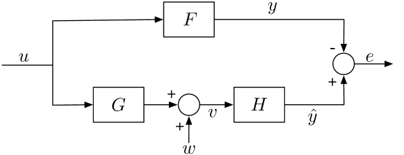
Figure 1: Approximation setup for differentially private filtering. The signal $w$ is a noise signal guaranteeing that $v$ is a differentially private signal. The signal $\hat{y}$ is differentially private no matter what the system $H$ is, see [15, Theorem 1].

IV-A SIMO system approximation

First, let us assume that $F$ on Fig. 1 is a SIMO filter, with $p$ outputs. Consider a first stage $G(z)=\text{col}(G_{1}(z),\ldots,G_{q}(z))$ taking the input signal $u$ and producing $q$ intermediate outputs that must be perturbed. The second stage is taken to be $H=FL$, with $L(z)=[L_{1}(z),\ldots,L_{q}(z)]$ a left-inverse of $G$, i.e., satisfying

$$\sum_{i=1}^{q}L_{i}(z)G_{i}(z)=1.$$

Let us also define the transfer functions $M_{i}$, $i=1,\ldots,q,$ such that $M_{i}(z)=L_{i}(z^{-1})$, hence $M_{i}(e^{j\omega})=L_{i}(e^{j\omega})^{*}$, and thus in particular

$$|M_{i}(e^{j\omega})|^{2}=|L_{i}(e^{j\omega})|^{2},i=1,\ldots,q,$$ (8)

and $$\sum_{i=1}^{q}M_{i}(e^{j\omega})^{*}G_{i}(e^{j\omega})=1.$$ (9)

From Theorem 2, the sensitivity of the first stage for input signals that are adjacent according to (1) is $k_{1}\|G\|_{2}$. Hence, according to Theorem 1, adding a white Gaussian noise $w$ to the output of $G$ with covariance matrix $k_{1}^{2}\kappa_{\delta,\epsilon}^{2}\|G\|_{2}^{2}I_{q}$ is sufficient to ensure that the signal $v$ on Fig. 1 is differentially private. The MSE for this mechanism can be expressed as

$$e^{ZFE}_{mse}(G) =\lim_{T\to\infty}\frac{1}{T}\sum_{t=0}^{\infty}\mathbb{E}\left[|(Fu)_{t}-(FLGu)_{t}-(FLw)_{t}|_{2}^{2}\right]$$

$$e^{ZFE}_{mse}(G) =\lim_{T\to\infty}\frac{1}{T}\sum_{t=0}^{\infty}\mathbb{E}\left[|(FLw)_{t}|_{2}^{2}\right]$$

$$e^{ZFE}_{mse}(G) =k_{1}^{2}\kappa_{\delta,\epsilon}^{2}\|G\|_{2}^{2}\|FL\|_{2}^{2}.$$

We are thus led to consider the minimization of $\|FL\|_{2}^{2}\|G\|_{2}^{2}$ over the pre-filters $G$. We have

$$\|FL\|_{2}^{2}\|G\|_{2}^{2} =\frac{1}{2\pi}\int_{-\pi}^{\pi}\text{Tr}(L^{*}(e^{j\omega})F^{*}(e^{j\omega})F(e^{j\omega})L(e^{j\omega}))d\omega\times\frac{1}{2\pi}\int_{-\pi}^{\pi}\text{Tr}(G^{*}(e^{j\omega})G(e^{j\omega}))d\omega$$

$$=\frac{1}{2\pi}\int_{-\pi}^{\pi}|F(e^{j\omega})|_{2}^{2}\;|L(e^{j\omega})|_{2}^{2}d\omega\times\frac{1}{2\pi}\int_{-\pi}^{\pi}|G(e^{j\omega})|_{2}^{2}d\omega$$

$$=\frac{1}{2\pi}\int_{-\pi}^{\pi}|F(e^{j\omega})|_{2}^{2}\;|M(e^{j\omega})|_{2}^{2}d\omega\times\frac{1}{2\pi}\int_{-\pi}^{\pi}|G(e^{j\omega})|_{2}^{2}d\omega,$$

where in the last equality we used (8). Now consider the following inner product on the space of $2\pi$-periodic functions with values in $\mathbb{C}^{q}$

$$\langle f,g\rangle=\frac{1}{2\pi}\int_{-\pi}^{\pi}f(e^{j\omega})^{*}g(e^{j\omega})d\omega.$$

By the Cauchy-Schwarz inequality for this inner product applied to the functions $\omega\mapsto|F(e^{j\omega})|_{2}M(e^{j\omega})$ and $\omega\mapsto G(e^{j\omega})$, we obtain the following bound

$$\|FL\|_{2}^{2}\|G\|_{2}^{2}\geq\left(\frac{1}{2\pi}\int_{-\pi}^{\pi}|F(e^{j\omega})|_{2}\sum_{i=1}^{q}M_{i}^{*}(e^{j\omega})G_{i}(e^{j\omega})d\omega\right)^{2},$$

i.e., using (9),

$$\|FL\|_{2}^{2}\|G\|_{2}^{2}\geq\left(\frac{1}{2\pi}\int_{-\pi}^{\pi}|F(e^{j\omega})|_{2}\,d\omega\right)^{2}.$$

Moreover, the two sides in the Cauchy-Schwarz inequality are equal, i.e., the bound is attained, if

$$|F(e^{j\omega})|_{2}M(e^{j\omega})=G(e^{j\omega}).$$

Note that this condition does not depend on $q$. Hence we can simply take $q=1$, and $L(z)=1/G(z)$, to get

$$|F(e^{j\omega})|_{2}\;L^{*}(e^{j\omega})=G(e^{j\omega})$$

$$\text{i.e., }|G(e^{j\omega})|^{2}=|F(e^{j\omega})|_{2}.$$ (10)

Finding $G$ SISO satisfying (10) is a spectral factorization problem. We can choose $G$ stable and minimum phase, so that its inverse $L$ is also stable. The following theorem summarizes the preceding discussion and generalizes [15, Theorem 8].

Theorem 6.

Let $F$ be a SIMO LTI system with $\|F\|_{2}<\infty$. For any stable LTI system $G$,

$$e^{ZFE}_{mse}(G)\geq k_{1}^{2}\kappa_{\delta,\epsilon}^{2}\left(\frac{1}{2\pi}\int_{-\pi}^{\pi}|F(e^{j\omega})|_{2}\;d\omega\right)^{2}.$$ (11)

If moreover $F$ satisfies the Paley-Wiener condition $\frac{1}{2\pi}\int_{-\pi}^{\pi}\ln|F(e^{j\omega})|_{2}\;\,d\omega>-\infty$, this lower bound on the mean square error of the ZFE mechanism can be attained by some stable minimum phase SISO system $G$ such that $|G(e^{j\omega})|^{2}=|F(e^{j\omega})|_{2}$, for almost every $\omega\in[-\pi,\pi)$.

Proof.

The main argument for the proof was given before the theorem. Since $|F(e^{j\omega})|_{2}$ is a nonnegative function on the unit circle, if it satisfies the Paley-Wiener condition, it has indeed a minimum phase spectral factor $G$ satisfying (10) almost everywhere [33, p. 242]. ∎

IV-B MIMO system approximation

Let us now assume that $F$ has $m>1$ inputs. We write $F(z)=[F_{1}(z),\ldots,F_{m}(z)]$, with $F_{i}$ a $p\times 1$ transfer matrix. In this case, in view of the complicated expression (7) for the sensitivity of a general MIMO filter, we only provide a subpotimal ZFE mechanism, together with a comparison between the performance of our mechanism and the optimal ZFE mechanism. The idea is to restrict our attention to pre-filters $G$ that are $m\times m$ and diagonal, for which the sensitivity is given in Theorem 3. The problem of optimizing the diagonal pre-filters, using the architecture depicted on Fig. 2, can in fact be seen as designing $m$ SIMO mechanisms.

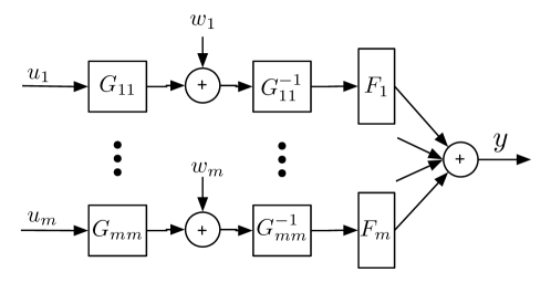
Figure 2: (Suboptimal) ZFE mechanism for a MIMO system $Fu=\sum_{i=1}^{m}F_{i}u_{i}$, and a diagonal pre-filter $G(z)=\text{diag}(G_{11}(z),\ldots,G_{mm}(z))$. Here $F_{i}(z)$ is a $p\times 1$ transfer matrix, for $i=1,\ldots,m$. The signal $w$ is a white Gaussian noise with covariance matrix $\kappa_{\delta,\epsilon}^{2}\|KG\|_{2}^{2}I_{m}$.

IV-B1 Diagonal Pre-filter Optimization

If $G$ is diagonal, then according to Theorem 3 its squared sensitivity is $(\Delta^{m,m}_{2}G)^{2}=\|KG\|_{2}^{2}=\sum_{i=1}^{m}\|k_{i}G_{ii}\|_{2}^{2}$, with $K=\text{diag}(k_{1},\ldots,k_{m})$. Following the same reasoning as in the previous subsection, the MSE for this mechanism can be expressed as

$$e^{ZFE}_{mse}(G) =\kappa_{\delta,\epsilon}^{2}\|KG\|_{2}^{2}\|FG^{-1}\|_{2}^{2},$$ (12)

with $G^{-1}(z)=\text{diag}(G_{11}(z)^{-1},\ldots,G_{mm}(z)^{-1})$. Now remark that

$$\|FG^{-1}\|_{2}^{2}=\frac{1}{2\pi}\int_{-\pi}^{\pi}\sum_{i=1}^{m}\frac{|F_{i}(e^{j\omega})|_{2}^{2}}{|G_{ii}(e^{j\omega})|^{2}}d\omega.$$

Hence from the Cauchy-Schwarz inequality again, we obtain the lower bound

$$e^{ZFE}_{mse}(G) \geq\kappa_{\delta,\epsilon}^{2}\left(\frac{1}{2\pi}\int_{-\pi}^{\pi}\sum_{i=1}^{m}\frac{|F_{i}(e^{j\omega})|_{2}}{|G_{ii}(e^{j\omega})|}|k_{i}G_{ii}(e^{j\omega})|d\omega\right)^{2}$$

$$e^{ZFE}_{mse}(G) \geq\kappa_{\delta,\epsilon}^{2}\left(\frac{1}{2\pi}\int_{-\pi}^{\pi}\sum_{i=1}^{m}k_{i}|F_{i}(e^{j\omega})|_{2}\;d\omega\right)^{2},$$

and this bound is attained if

$$k_{i}|G_{ii}(e^{j\omega})| =\frac{|F_{i}(e^{j\omega})|_{2}}{|G_{ii}(e^{j\omega})|},$$

$$\text{i.e. }\;k_{i}|G_{ii}(e^{j\omega})|^{2} =|F_{i}(e^{j\omega})|_{2},\;i=1,\ldots,m.$$

In other words, the best diagonal pre-filter for the MIMO ZFE mechanism can be obtained from $m$ spectral factorizations of the functions $\omega\mapsto\frac{1}{k_{i}}|F_{i}(e^{j\omega})|_{2}$, $i=1,\ldots,m$.

Theorem 7.

Let $F=[F_{1},\ldots,F_{m}]$ be a MIMO LTI system with $\|F\|_{2}<\infty$. We have, for any stable diagonal filter $G(z)=\text{diag}(G_{11}(z),\ldots,G_{mm}(z))$,

$$e^{ZFE}_{mse}(G)\geq\kappa_{\delta,\epsilon}^{2}\left(\frac{1}{2\pi}\int_{-\pi}^{\pi}\sum_{i=1}^{m}k_{i}|F_{i}(e^{j\omega})|_{2}\;d\omega\right)^{2}.$$ (13)

If moreover each $F_{i}$ satisfies the Paley-Wiener condition $\frac{1}{2\pi}\int_{-\pi}^{\pi}\ln|F_{i}(e^{j\omega})|_{2}\,d\omega>-\infty$, this lower bound on the mean-squared error of the ZFE mechanism can be attained by some stable minimum phase systems $G_{ii}$ such that $|G_{ii}(e^{j\omega})|^{2}=\frac{1}{k_{i}}|F_{i}(e^{j\omega})|_{2}$, for almost every $\omega\in[-\pi,\pi)$.

Remark 1.

Note that the integrand on the right-hand side of (14) can be written

$$\sum_{i=1}^{m}k_{i}|F_{i}(e^{j\omega})|_{2}:=\|F(e^{j\omega})K\|_{2,1},$$

where $K=\text{diag}(k_{1},\ldots,k_{m})$ as usual and $\|\cdot\|_{2,1}$ is the so-called $L_{2,1}$ or $R_{1}$ matrix norm, and appears in [34] for example.

IV-B2 Comparison with Non-Diagonal Pre-filters

For $F$ a general MIMO system, it is possible that we could achieve a better performance with a ZFE mechanism where $G$ is not diagonal, i.e., by combining the inputs before adding the privacy-preserving noise. To provide a better understanding of how much could potentially be gained by carrying out this more involved optimization over general pre-filters $G$ rather than just diagonal pre-filters, the following Theorem provides a a lower bound on the MSE achievable by any ZFE mechanism.

Theorem 8.

Let $F=[F_{1},\ldots,F_{m}]$ be a MIMO LTI system with $\|F\|_{2}<\infty$. We have, for any $m\times m$ stable filter $G(z)$, with left inverse $L$ so that $L(z)G(z)=I$,

$$e^{ZFE}_{mse}(G)\geq\kappa_{\delta,\epsilon}^{2}\left(\frac{1}{2\pi}\int_{-\pi}^{\pi}\|F(e^{j\omega})K\|_{*}d\omega\right)^{2},$$ (14)

where $\|F(e^{j\omega})K\|_{*}$ denotes the nuclear norm of the matrix $F(e^{j\omega})K$ (sum of singular values).

The lower bound (15) on the achievable MSE with a general pre-filter in a ZFE mechanism should be compared to the performance (14) that can actually be achieved with diagonal pre-filters. Note that these bounds coïncide for $m=1$. For $m>1$, the gap depends on the difference between the integrals of the $L_{2,1}$ norm and the nuclear norm of $F(e^{j\omega})K$.

Proof.

We denote as usual $K=\text{diag}(k_{1},\ldots,k_{m})$, and define $\tilde{G}=GK$ and $\tilde{L}=K^{-1}L$, so that we again have $\tilde{L}\tilde{G}=I$. Let $\tilde{F}=FK$. With the lower bound of Theorem 4, designing a ZFE mechanism based on sensitivity as above would require adding a noise with variance at least $\kappa_{\delta,\epsilon}^{2}\|\tilde{G}\|_{2}^{2}$. This would lead to an MSE at least equal to $\kappa_{\delta,\epsilon}^{2}\|\tilde{G}\|_{2}^{2}\|\tilde{F}\tilde{L}\|_{2}^{2}$. Now note that

$$\|\tilde{F}\tilde{L}\|_{2}^{2} =\frac{1}{2\pi}\int_{-\pi}^{\pi}\text{Tr}(\tilde{F}(e^{j\omega})\tilde{L}(e^{j\omega})\tilde{L}(e^{j\omega})^{*}\tilde{F}(e^{j\omega})^{*})d\omega$$

$$=\frac{1}{2\pi}\int_{-\pi}^{\pi}\text{Tr}(\tilde{F}(e^{j\omega})^{*}\tilde{F}(e^{j\omega})\tilde{L}(e^{j\omega})\tilde{L}(e^{j\omega})^{*})d\omega$$

$$=\frac{1}{2\pi}\int_{-\pi}^{\pi}\text{Tr}(A(e^{j\omega})^{2}\tilde{L}(e^{j\omega})\tilde{L}(e^{j\omega})^{*})d\omega$$

$$=\frac{1}{2\pi}\int_{-\pi}^{\pi}\text{Tr}(A(e^{j\omega})\tilde{L}(e^{j\omega})\tilde{L}(e^{j\omega})^{*}A(e^{j\omega}))d\omega,$$

where for all $\omega$, $A(e^{j\omega})$ is the unique Hermitian positive-semidefinite square root of $\tilde{F}(e^{j\omega})^{*}\tilde{F}(e^{j\omega})$, i.e., $A(e^{j\omega})^{2}=\tilde{F}(e^{j\omega})^{*}\tilde{F}(e^{j\omega})$. Then, once again from the Cauchy-Schwarz inequality, now for the inner product $\langle M,N\rangle=\frac{1}{2\pi}\int_{-\pi}^{\pi}\text{Tr}(M(e^{j\omega})^{*}N(e^{j\omega}))d\omega,$

$$\|GK\|_{2}^{2}\;\|FL\|_{2}^{2} =\|\tilde{G}\|_{2}^{2}\|\tilde{F}\tilde{L}\|_{2}^{2}=\left[\frac{1}{2\pi}\int_{-\pi}^{\pi}\text{Tr}(\tilde{G}(e^{j\omega})^{*}\tilde{G}(e^{j\omega}))d\omega\right]$$

$$\times\Bigg{[}\frac{1}{2\pi} \int_{-\pi}^{\pi}\text{Tr}(A(e^{j\omega})\tilde{L}(e^{j\omega})\tilde{L}(e^{j\omega})^{*}A(e^{j\omega}))d\omega\Bigg{]}$$

$$\geq\left(\frac{1}{2\pi}\int_{-\pi}^{\pi}\text{Tr}(A(e^{j\omega})\tilde{L}(e^{j\omega})\tilde{G}(e^{j\omega}))d\omega\right)^{2}$$

$$\text{and so }\;e^{ZFE}_{mse}(G) \geq\kappa_{\delta,\epsilon}^{2}\left(\frac{1}{2\pi}\int_{-\pi}^{\pi}\|F(e^{j\omega})K\|_{*}d\omega\right)^{2},$$ (15)

where $\|F(e^{j\omega})K\|_{*}=\text{Tr}(A(e^{j\omega}))$ denotes the nuclear norm of the matrix $F(e^{j\omega})K$. ∎

V Application to Privacy-Preserving Estimation of Building Occupancy

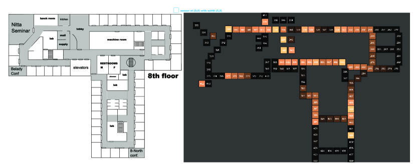
Figure 3: Left: plan of one of the two floors in the MERL building used for the sensor network experiment [35]. The shaded areas are hallways, lobbies and meeting rooms equipped with binary motion detection sensors, placed a few meters apart and recording events roughly every second. Right: a figure taken from [36] shows a visualisation of a crowd movement during a fire drill.

In this section we illustrate the design process and the performance of the ZFE mechanism in the context of an application to filtering and forecasting occupancy-related events in an office building equipped with motion detection sensors. As mentioned in Section II-B, such sensor networks raise privacy concerns since some occupants could potentially be tracked individually from the published information, especially when it is correlated with public information such as the location of their office. Since the amount of private information leakage depends on the output signals the system aims to generates, we adjust the privacy-preserving noise level based on the filter specification using the ZFE mechanism. As an example, we simulate the outputs of a $3\times 15$ MIMO filter processing input signals collected during a sensor network experiment carried out at the Mitsubishi Electric Research Laboratories (MERL) and described in [35] and on Fig. 3. We refer the reader to [36] for examples of identification of individual trajectories from this dataset.

The original dataset contains the traces of $213$ sensors placed a few meters apart and spread over two floors of a building, where each sensor recorded roughly every second and with millisecond accuracy over a year the exact times at which they detected some motion. For illustration purposes we downsampled the dataset in space and time, summing all the events recorded by several sufficiently close sensors over $3$ minute intervals. From this step, we obtained $15$ input signals $u_{i}$, $i=1,\ldots,15$, corresponding to $15$ spatial zones (each zone covered by cluster of about $14$ sensors), with a discrete-time period corresponding to $3$ minutes, and $u_{i,t}$ being the number of events detected by all the sensors in zone $i$ during period $t$. Let us assume say that during a given discrete-time period, a single individual can activate at most $4$ sensors in any group, hence $k_{i}=4$ for $1\leq i\leq 15$. Moreover, we need to assume that a single individual only activates the sensors in a given zone once over the time interval for which we wish to provide differential privacy. Section II-B discussed how to relax this requirement by splitting the input data into successive time windows and creating additional input channels.

For our example, we consider computing simultaneously and in real-time the following three outputs from the $15$ input signals

$$\begin{bmatrix}y_{1}\\ y_{2}\\ y_{3}\end{bmatrix}=\begin{bmatrix}f_{1}(z)\mathbf{1}_{1\times 5}\;\;\;\;\mathbf{0}_{1\times 10}\\ \mathbf{0}_{1\times 4}\;\;\;\;f_{2}(z)\mathbf{1}_{1\times 8}\;\;\;\;\mathbf{0}_{1\times 3}\\ f_{3}(z)\end{bmatrix}u,$$ (16)

where

• $y_{1}$ is the sum of the simple moving averages over the past $60$ min for zones $1$ to $5$, i.e., $f_{1}(z)=\frac{1}{20}\sum_{k=1}^{20}z^{-k}$,

• $y_{2}$ is $\sum_{i=5}^{12}f_{2}u_{i}$, with $f_{2}$ a finite impulse response low-pass filter with Gaussian shaped impulse response of length $20$, obtained using Matlab’s function gaussdesign(0.5,2,10).

• $y_{3}$ is the scalar output of a $1\times 15$ MISO filter $f_{3}$ designed to forecast at each period $t$ the average total number of events per time-period that will occur in the whole building during the window $[t+60\text{ min},t+90\text{ min}]$. This filter was constructed by identifying an ARMAX model [37] between the $15$ inputs (plus a scalar white noise) and the desired outputs, with the calibration done using one part of the dataset. The model chosen is takes the form

  $$y_{3,t}=\sum_{i=1}^{4}a_{i}y_{3,t-i}+b_{0}u_{t}+b_{1}u_{t-2}+c_{1}e_{t},$$

  where $a_{1},\ldots,a_{4}$ and $b_{0},b_{1}$ are scalar and row vectors respectively forming the filter $f_{3}$, $c_{1}$ is a scalar and $e_{t}$ is a zero-mean white noise input postulated by the ARMAX model for system identification purposes.

Fig. 4 shows sample paths over a $72$h period of the $2$nd and $3$rd outputs of the desired filter and of its ($\ln 5,0.05$)-differentially private approximation obtained using the ZFE mechanism. The $15$ optimal pre-filters were obtained approximately via least-squares fit of $\sqrt{|F_{i}(e^{j\omega})|_{2}}$ with negligible approximation error (Matlab’s function yulewalk implementing the Yule-Walker method [38]), rather than true spectral factorization mentioned in Theorem 7. One apparent aspect of the privacy-preserving outputs seen on Fig. 4 is that the noise level is independent of the size of the desired output signal, hence low signal values tend to be easily buried in the noise. This is one drawback of mechanisms relying on global sensitivity measures and additive noise. Another noticeable element is the fact that the noise remaining on each output can have quite different characteristics depending on the desired filter $F$, with the post-filter $FG^{-1}$ removing more high-frequency components on the second output than on the third.

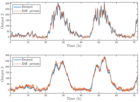
Figure 4: Sample-paths over $72$ hours (the sampling period is $3$ min) for the outputs $2$ and $3$ of our differentially private approximation of filter (16), shown together with the desired outputs. The privacy-related parameters are $\epsilon=\ln 5,\delta=0.05,k_{i}=4$ for $1\leq i\leq 15$.

VI Exploiting Additional Information on the Input Signals

The main issue with SISO zero-forcing equalizers is the noise amplification at frequencies where $|G(e^{j\omega})|$ is small, due to the inversion in $H=FG^{-1}$ [39]. This issue is not as problematic for the optimal ZFE mechanism, since in this case the amplification is compensated by the fact that $|F(e^{j\omega})|$ and $|G(e^{j\omega})|$ given in Theorem 7 are both small at the same frequencies. Nonetheless, we expect to be able to improve on the ZFE mechanism by using more advanced equalization schemes in the design of $H$. In this section the choice of post-filter $H$ of Fig. 1 depends on certain input signal properties, and we concentrate on the optimization of diagonal pre-filters $G$ as for the ZFE mechanism. Note however that the mechanisms below require that the input signals satisfy certain constraints, such as wide-sense stationarity, and that some publicly available information on these signals be available, e.g., their second order statistics. Hence, the ZFE mechanism remains generally useful due to its broad applicability.

VI-A Exploiting Information on Second-Order Statistics with Linear Mean Square Mechanisms

First, one can improve on the ZFE mechanism if some information on the statistics of the input signal $u$ is publicly available. In general, constructing the optimum maximum-likelihood estimate of $\{(Fu)_{k}\}_{k\geq 0}$ from $\{v_{k}\}_{k\geq 0}$ on Fig. 1 is computationally intensive and requires the knowledge of the full joint probability distribution of $\{u_{k}\}_{k\geq 0}$ [39]. Hence, we explore in this subsection a simpler scheme based on linear minimum mean square error estimation, which we call the Linear Mean Square (LMS) mechanism.

To develop the LMS mechanism, we assume that it is publicly known that $u$ is wide-sense stationary (WSS) with know mean vector $\mu$ and matrix-valued autocorrelation sequence $R_{u}[k]=\mathbb{E}[u_{t}u^{T}_{t-k}]=R_{u}[-k]^{T},\forall k$. Since the mean of the output $y$ is then known, equal to $F(1)\mu$, we can assume without loss of generality that $\mu=0$. The $z$-spectrum of $u$, $P_{u}(z)=\sum_{k=-\infty}^{\infty}R_{u}[k]z^{-k}$, is assumed for simplicity of exposition to be rational and positive definite on the unit circle, i.e., for $z=e^{j\omega}$. More generally, given two vector-valued WSS zero-mean signals $u$ and $v$, we denote the cross-correlation matrix $R_{uv}[k]=\mathbb{E}[u_{t}v^{T}_{t-k}]$, the cross z-spectrum $P_{uv}(z)=\sum_{k=-\infty}^{\infty}R_{uv}[k]z^{-k}$, and all $z$-spectra are assumed to be rational.

The design of the LMS mechanism relies on a Wiener filter $H$ to estimate $y$ from $v$ on Fig. 1 [40, 33]. Recall that the Wiener filter produces an estimate $\hat{y}$ minimizing the MSE between $y$ and $\hat{y}$ over linear filters, assuming that the signal $v$ is stationary. Its design requires the knowledge of the second-order statistics of $v$, which can be expressed in terms of those of $u$, $w$, and of the transfer function $G$. Our design procedure involves the following steps. First, for tractability reasons, we assume initially that $H$ is an infinite impulse response (IIR) Wiener smoother, i.e., non-causal. The reason is that we can then express the estimation performance analytically as a function of $G$. We then optimize this performance measure over diagonal pre-filters $G$. Once $G$ is fixed, real-time considerations force us to use a lower-performance design with $H$ a causal Wiener filter, or perhaps a slightly non-causal filter introducing a small delay is tolerable for a specific application.

VI-A1 Diagonal Pre-Filter Optimization

The (non-causal) Wiener smoother $H$ has the transfer function $H(z)=P_{yv}(z)P_{v}(z)^{-1}$ [40, Section 7.8]. According to Theorem 3, for $G$ diagonal we can take the privacy-preserving noise $w$ to be white and Gaussian with covariance $\sigma^{2}I_{m}$ with $\sigma^{2}=\kappa_{\delta,\epsilon}^{2}\|GK\|_{2}^{2}$. Since $u$ and $w$ are uncorrelated, we have

$$P_{yv}(z)=F(z)P_{u}(z)G(z^{-1})^{T},\,\,P_{v}(z)=G(z)P_{u}(z)G(z^{-1})^{T}+\sigma^{2}I_{m}.$$ (17)

Hence

$$H(z)=F(z)P_{u}(z)G(z^{-1})^{T}\left(G(z)P_{u}(z)G(z^{-1})^{T}+\kappa_{\delta,\epsilon}^{2}\|G\|_{2}^{2}\,I_{m}\right)^{-1}.$$ (18)

The MSE can then be expressed as $e^{lms}(G)=\frac{1}{2\pi}\int_{-\pi}^{\pi}\text{Tr}(P_{y}(e^{j\omega})-P_{\hat{y}}(e^{j\omega}))d\omega$ [40, Chapter 7]. In our case,

$$P_{\hat{y}}(e^{j\omega}) =H(e^{j\omega})P_{v}(e^{j\omega})H(e^{j\omega})^{*}=P_{yv}(e^{j\omega})P_{v}(e^{j\omega})^{-1}P_{yv}(e^{j\omega})^{*}$$

$$P_{\hat{y}} =FP_{u}G^{*}(\sigma^{2}I_{m}+GP_{u}G^{*})^{-1}GP_{u}F^{*},$$

where on the second line and below we omit the argument $e^{j\omega}$ next to all matrices, to simplify the notation. We have then

$$P_{y}-P_{\hat{y}} =FP_{u}F^{*}-P_{\hat{y}}=F(P_{u}-P_{u}G^{*}(\sigma^{2}I_{m}+GP_{u}G^{*})^{-1}GP_{u})F^{*}$$

$$=F\left(P_{u}^{-1}+\frac{1}{\sigma^{2}}G^{*}G\right)^{-1}F^{*},$$

with the last expression obtained using the matrix inversion lemma. Finally, defining $\tilde{G}(e^{j\omega}):=\frac{1}{\|GK\|_{2}}G(e^{j\omega})K$, we obtain the expression

$$e^{lms}(\tilde{G}) =\frac{1}{2\pi}\int_{-\pi}^{\pi}\text{Tr}\left[F(e^{j\omega})\left(P_{u}(e^{j\omega})^{-1}+\frac{1}{\kappa_{\delta,\epsilon}^{2}}K^{-1}\tilde{G}(e^{j\omega})^{*}\tilde{G}(e^{j\omega})K^{-1}\right)^{-1}F^{*}(e^{j\omega}))\right]d\omega$$

$$e^{lms}(\tilde{G}) =\frac{1}{2\pi}\int_{-\pi}^{\pi}\text{Tr}\left[\tilde{F}(e^{j\omega})(\tilde{P}_{u}(e^{j\omega})^{-1}+\tilde{G}(e^{j\omega})^{*}\tilde{G}(e^{j\omega}))^{-1}\tilde{F}(e^{j\omega})^{*}\right]d\omega,$$ (19)

where $\tilde{F}(e^{j\omega})=\kappa_{\delta,\epsilon}F(e^{j\omega})K$ and $\tilde{P}_{u}(e^{j\omega})=\frac{1}{\kappa_{\delta,\epsilon}^{2}}K^{-1}P_{u}(e^{j\omega})K^{-1}$. The objective (19) should be minimized over all transfer functions $\tilde{G}$, which by definition must satisfy the constraint

$$\|\tilde{G}\|^{2}_{2}=\frac{1}{2\pi}\int_{-\pi}^{\pi}\text{Tr}(\tilde{G}(e^{j\omega})^{*}\tilde{G}(e^{j\omega}))d\omega=1.$$ (20)

Note that in (19) we recover the expression (12) of the performance of the ZFE mechanism in the limit $\tilde{P}_{u}(e^{j\omega})\to\infty$.

It remains to minimize the performance measure (19) over the choise of pre-filters $G$ satisfying (20). First, in the case where $\tilde{P}_{u}(e^{j\omega})$ or equivalently $P_{u}(e^{j\omega})$ is diagonal for all $\omega$, i.e., the different input signals are uncorrelated, we have in fact a classical allocation problem [41] whose solution is of the “waterfilling type”. Namely, denote $\tilde{P}_{u}(e^{j\omega})=\text{diag}(p_{1}(e^{j\omega}),\ldots,p_{m}(e^{j\omega}))$ and $X(e^{j\omega})=\tilde{G}(e^{j\omega})^{*}\tilde{G}(e^{j\omega})=\text{diag}(x_{1}(e^{j\omega}),\ldots,x_{m}(e^{j\omega}))$, with $x_{i}(e^{j\omega})=|\tilde{g}_{ii}(e^{j\omega})|^{2}$. Omitting the expression $e^{j\omega}$ in the integrals for clarity, (19) and (20) read

$$\min_{x}\frac{1}{2\pi}\int_{-\pi}^{\pi}\sum_{i=1}^{m}\frac{1}{\frac{1}{p_{i}}+x_{i}}|\tilde{F}_{i}|_{2}^{2}\,d\omega\text{ s.t. }\frac{1}{2\pi}\int_{-\pi}^{\pi}\sum_{i=1}^{m}x_{i}\,d\omega=1,\;\;x_{i}(e^{j\omega})\geq 0,\forall\omega,i,$$

and the solution to this convex problem is

$$x_{i}(e^{j\omega})=\max\left\{0,\sqrt{\frac{|\tilde{F}_{i}(e^{j\omega})|_{2}^{2}}{\lambda}}-\frac{1}{p_{i}(e^{j\omega})}\right\},$$

where $\lambda>0$ is adjusted so that the solution satisfies the equality constraint (20). Problems of this type are discussed in the communication literature on joint transmitter-receiver optimization [27, 28], which is not too surprising in view of our approximation setup on Fig. 1.

When $\tilde{P}_{u}(e^{j\omega})$ is not diagonal, it is shown in [28] that the problem can be reduced to the diagonal case if $\tilde{G}$ can be arbitrary, however the argument does not carry through under our constraint that $\tilde{G}$ must also be diagonal. Nonetheless, one can obtain a solution arbitrarily close to the optimal one using semidefinite programming. First, we discretize the optimization problem at the set of frequencies $\omega_{q}=\frac{q\pi}{N},q=0\ldots N$. Note that all functions are even functions of $\omega$, hence we can restrict out attention to the interval $[0,\pi]$. Then, we define the $m(N+1)$ variables $x_{iq}=x_{i}(e^{j\omega_{q}})$, with $x_{iq}\geq 0$, and $X_{q}=\text{diag}(x_{1q},\ldots,x_{mq})$. Using the trapezoidal rule to approximate the integrals, we obtain the following optimization problem

$$\min_{\{X_{q},M_{q}\}_{0\leq q\leq N}}\quad \frac{1}{2N}\sum_{q=0}^{N-1}\text{Tr}\left[M_{q}+M_{q+1}\right]$$ (21)

s.t. $$\begin{bmatrix}M_{q}&\tilde{F}_{q}\\ \tilde{F}_{q}^{*}&\tilde{P}_{q}^{-1}+X_{q}\end{bmatrix}\succeq 0,\;\;0\leq q\leq N,$$ (22)

$$\frac{1}{2N\pi}\sum_{q=0}^{N-1}\text{Tr}[X_{q}+X_{q+1}]=1,\text{ and }X_{q}\succeq 0,\;\;0\leq q\leq N,$$

where $\tilde{F}_{q}:=\tilde{F}(e^{j\omega_{q}})$ and $\tilde{P}_{q}=\tilde{P}_{u}(e^{j\omega_{q}})$. Note that (22) is equivalent to $M_{q}\succeq\tilde{F}_{q}(\tilde{P}_{q}^{-1}+X_{q})^{-1}\tilde{F}_{q}^{*}$ by taking the Schur complement. The optimization problem (22) is a semidefinite program, and can thus be solved efficiently even for relatively fine discretizations of the interval $[0,\pi]$. The transfer functions $\tilde{g}_{ii}$ (and hence $g_{ii}$) of the filter $\tilde{G}$ can then be obtained by interpolation of the squared magnitude $x_{i}(e^{j\omega})$ from the $x_{iq}$ and $m$ spectral factorizations.

Remark 2.

Even if the statistical assumptions on $u$ turn out not to be correct, and even though the optimization problem is solved approximately rather than exactly, the differential privacy guarantee of the LMS mechanism still holds and only the approximation quality is impacted.

VI-A2 Causal Mechanism

Once the diagonal pre-filter $G$ is computed by the optimization procedure described above, we construct the final mechanism by replacing the smoother $H$ from (18) by a filter respecting the causality or delay constraints of the application. Note from (17) that $P_{v}(e^{j\omega})\succ 0$ for all $-\pi\leq\omega<\pi$. Denote the canonical spectral factorization $P_{v}(z)=L(z)P_{e}L(z^{-1})^{T}$ where $P_{e}\succ 0$ and $L$ and $L^{-1}$ are analytic in the region $|z|\geq 1$ and $L(\infty)=I_{m}$ [40, Section 7.8]. Then the causal Wiener filter is $H(z)=[P_{yv}(z)L(z^{-1})^{-T}]_{+}\,P_{e}^{-1}L(z)^{-1},$ where for a linear filter $M(z)$ with (matrix-valued) impulse reponse $\{M_{t}\}_{-\infty\leq t\leq\infty}$, $[M(z)]_{+}$ denotes the causal filter with impulse response $\{M_{t}\mathbf{1}_{\{t\geq 0\}}\}_{t}$.

VI-B Exploiting Information on the Input Domain using Decision-Feedback Mechanisms

Signals capturing event streams often take values in a discrete set, e.g., if they originate from various counting sensors as in Section V. This information can be taken into account together with the previous statistical information by introducing a slight degree of nonlinearity in the LMS mechanism, using the idea of decision-feedback equalization [39]. We call the resulting mechanism presented below a Decision-Feedback (DF) mechanism. Its architecture is depicted on Fig. 5. Note that compared to the optimal Wiener smoother (18) in the previous section, which is of the form $FH_{u}$, the only structural difference is the presence of the decision block and the feedback loop.

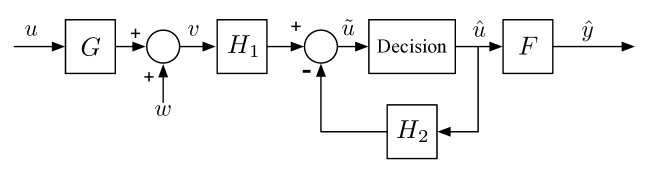
Figure 5: Decision-feedback mechanism. The decision block is nonlinear and depends on the information about the domain of the input signal $u$, operating as a detector or quantizer for example.

The first stage of the DF mechanism is a pre-filter whose sensitivity determines as usual the amount of privacy-preserving noise $w$ to add. The second stage consists of a forward filter $H_{1}$, a nonlinear decision procedure (detector or quantizer) to estimate $u$ from $\tilde{u}$, which exploits the fact that $u$ takes discrete values, and a filter $H_{2}$ that feeds back the previous symbol decisions to correct the intermediate estimate $\tilde{u}$. $H_{2}$ is assumed to be strictly causal, but $H_{1}$ is often taken to be at least slightly non-causal in standard DF equalizers, for better performance [42]. In this case the mechanism will introduce a small delay in the publication of the output signal $\hat{y}$. In the absence of detailed information about the distribution of $u$, the decision device can be a simple quantizer for integer valued input sequences, or a detector $\hat{u}_{k}=\texttt{sign}(\tilde{u}_{k})$ for input sequences taking values in $\{-1,+1\}$.

The error between the desired output $Fu$ and the signal $F\tilde{u}$, where $\tilde{u}$ is the input of the detector, is $e=F(u-\tilde{u})=F(u-H_{1}v+H_{2}\hat{u})$. For tractability reasons, the analysis and design of DF equalizers is usually carried out under the simplifying assumption that the past decisions entering $H_{2}$ are correct, i.e., that $\hat{u}_{k}=u_{k}$. In this case, the error reads

$$e\approx F((B-H_{1}G)u-H_{1}w),$$

with $B(z)=I+H_{2}(z)$ a monic filter (i.e., $B_{0}=I$) since $H_{2}$ is strictly causal. For a given $B$, the system $H_{1}$ minimizing the MSE is again the Wiener smoother to estimate $Bu$ from $Gu+w$, i.e., comparing with (18), (19)

$$H_{1}(z) =B(z)P_{u}(z)G(z^{-1})^{T}\left(G(z)P_{u}(z)G(z^{-1})^{T}+\kappa_{\delta,\epsilon}^{2}\|G\|_{2}^{2}\,I_{m}\right)^{-1},$$

$$e^{df}(B,\tilde{G}) =\frac{\kappa_{\delta,\epsilon}^{2}}{2\pi}\int_{-\pi}^{\pi}\text{Tr}\left[F(e^{j\omega})B(e^{j\omega})K(\tilde{P}_{u}(e^{j\omega})^{-1}+\tilde{G}(e^{j\omega})^{*}\tilde{G}(e^{j\omega}))^{-1}KB(e^{j\omega})^{*}F(e^{j\omega})^{*}\right]d\omega.$$

The next step is to optimize over the monic filter $B$. First, consider the spectral factorizations

$$K(\tilde{P}_{u}(e^{j\omega})^{-1}+\tilde{G}(e^{j\omega})^{*}\tilde{G}(e^{j\omega}))^{-1}K=Q(e^{j\omega})RQ(e^{j\omega})^{*}$$ (23)

$$F(e^{j\omega})^{*}F(e^{j\omega})=S(e^{j\omega})^{*}TS(e^{j\omega}),$$ (24)

with $Q,S$ monic, causal, stable and invertible filters, and $R,T$ positive definite matrices. We have

$$e^{df}(B,\tilde{G}) =\frac{\kappa_{\delta,\epsilon}^{2}}{2\pi}\int_{-\pi}^{\pi}\text{Tr}\left[B(e^{j\omega})Q(e^{j\omega})RQ(e^{j\omega})^{*}B(e^{j\omega})^{*}S(e^{j\omega})^{*}TS(e^{j\omega})\right]d\omega$$

$$=\frac{\kappa_{\delta,\epsilon}^{2}}{2\pi}\int_{-\pi}^{\pi}\text{Tr}\left[T^{1/2}S(e^{j\omega})B(e^{j\omega})Q(e^{j\omega})RQ(e^{j\omega})^{*}B(e^{j\omega})^{*}S(e^{j\omega})^{*}T^{1/2}\right]d\omega$$

$$=\kappa_{\delta,\epsilon}^{2}\|T^{1/2}SBQR^{1/2}\|_{2}^{2}.$$

Note that $SBQ$ is a monic, stable and causal filter. We have the following lemma.

Lemma 1.

If $G(z)=\sum_{k\geq 0}G_{k}z^{-k}$ be a monic ($G_{0}=I$), stable and causal filter. Let $T$, $R$ be positive definite Hermitian matrices. Then

$$\|T^{1/2}GR^{1/2}\|^{2}_{2}\geq\text{Tr}(TR),$$

with equality attained when $G=\text{Id}$, i.e., $G_{k}=0$ for $k\geq 1$.

Proof.

We have

$$\|T^{1/2}GR^{1/2}\|^{2}_{2} =\frac{1}{2\pi}\int_{\pi}^{\pi}\text{Tr}\left[T^{1/2}G(e^{j\omega})RG^{*}(e^{j\omega})T^{1/2}\right]d\omega$$

$$=\text{Tr}\left(\sum_{k\geq 0}T^{1/2}G_{k}RG^{*}_{k}T^{1/2}\right)\;\;(\text{Parceval identity})$$

$$=\text{Tr}(TR)+\text{Tr}\left(\sum_{k>0}T^{1/2}G_{k}RG^{*}_{k}T^{1/2}\right)$$

$$\geq\text{Tr}(TR),$$

since the terms in the last sum are positive semi-definite matrices. Clearly equality is attained for $G_{k}=0$ for $k\geq 1$. ∎

From Lemma 1 we deduce immediately that we should choose

$$B(z)=S^{-1}(z)Q^{-1}(z)$$

and the corresponding MSE is $e^{df}(\tilde{G})=\kappa_{\delta,\epsilon}^{2}\,\text{Tr}(TR)$, with the positive definite matrices $T,R$ defined in (23), (24).

The final step would be to optimize the filter $G$ to minimize this expression of $e^{df}$. Although this can be done using an approach similar to the one of the Section VI-A, see [43, 1], it appears that this procedure in general results in a pre-filter $G$ that does not depend on the query $F$, which could be an artifact of the initial assumption that past decisions are correct. This can be seen most easily in the single-input case where $T,R$ are positive scalars, so that $e^{df}(\tilde{G})=TR$. In this product $F$ influences only in the factor $T$ and $G$ only in the factor $R$, hence the minimization over $G$ does not depend on $F$. Optimizing $G$ independently of $F$ appears to lead to suboptimal designs in general, see [1].

Hence, we propose the following design strategy for DF mechanisms. Note from (18) that the (non-causal) LMS mechanism involves a Wiener smoother $H(z)=F(z)H_{u}(z)$, with $H_{u}$ the Linear Minimum Mean Squared Error estimator for $u$. We can interpret the DF mechanism on Fig. 5 as introducing an additional (nonlinear) stage to the LMS mechanisms to discretize the estimate of $u$, and replacing $H_{u}$ by $H_{1}$. A (potentially suboptimal) strategy to improve on the performance of the LMS (or ZFE) mechanism is then to keep the same prefilter $G$ designed in Section VI-A, but simply replace the Wiener smoother or filter by the decision-feedback equalizer as described above, with a causal or almost causal approximation of the filter $H_{1}$. Our simulation results tend to confirm that good performance is achievable with this strategy.

Remark 1.

Other DF mechanisms are possible. For example, $H_{1}$ could be chosen as a zero-forcing ($H_{1}=G^{-1}$ in the SISO case) rather than a mean square equalizer, see, e.g., [44].

VII Conclusion

We have described a two-stage optimization procedure that can be used in the filtering of event streams in order to minimize the impact on performance of a differential privacy specification. The architecture considered here for the privacy-preserving mechanisms decomposes into a standard equalization or estimation problem, for which many alternatives techniques could be used depending on the scenario, and a first-stage privacy-preserving filter optimization problem. This two-stage design allows us to balance the privacy constraint and performance, and appears to be in fact quite general and even applicable to other definitions of privacy. Current work includes extending it to the design of differentially private nonlinear filters [45].

References

- [1] J. Le Ny, “On differentially private filtering for event streams,” in Proceedings of the 52nd Conference on Decision and Control, Florence, Italy, December 2013.
- [2] J. Le Ny and M. Mohammady, “Differentially private MIMO filtering for event streams and spatio-temporal monitoring,” in Proceedings of the 53rd Conference on Decision and Control, Los Angeles, CA, December 2014.
- [3] R. H. Weber, “Internet of things - new security and privacy challenges,” Computer Law and Security Review, vol. 26, pp. 23–30, 2010.
- [4] President’s Council of Advisors on Science and Technology, “Big data and privacy: A technological perspective,” Report to the President, Executive Office of the President of the United States, Tech. Rep., May 2014.
- [5] Electronic privacy information center. Online: http://epic.org/.
- [6] H. Chan and A. Perrig, “Security and privacy in sensor networks,” Computer, vol. 36, no. 10, pp. 103–105, Oct 2003.
- [7] G. Duncan and D. Lambert, “Disclosure-limited data dissemination,” Journal of the American Statistical Association, vol. 81, no. 393, pp. 10–28, March 1986.
- [8] L. Sweeney, “k-anonymity: A model for protecting privacy,” International Journal of Uncertainty, Fuzziness and Knowledge-Based Systems, vol. 10, no. 05, pp. 557–570, 2002.
- [9] L. Sankar, S. R. Rajagopalan, and H. V. Poor, “A theory of privacy and utility in databases,” Princeton University, Tech. Rep., February 2011.
- [10] M. Xue, W. Wang, and S. Roy, “Security concepts for the dynamics of autonomous vehicle networks,” Automatica, vol. 50, pp. 852–857, 2014.
- [11] N. E. Manitara and C. N. Hadjicostis, “Privacy-preserving asymptotic average consensus,” in Proceedings of the European Control Conference, 2013.
- [12] C. Dwork, F. McSherry, K. Nissim, and A. Smith, “Calibrating noise to sensitivity in private data analysis,” in Proceedings of the Third Theory of Cryptography Conference, 2006, pp. 265–284.
- [13] C. Dwork, “Differential privacy,” in Proceedings of the 33rd International Colloquium on Automata, Languages and Programming (ICALP), ser. Lecture Notes in Computer Science, vol. 4052. Springer-Verlag, 2006.
- [14] J. Le Ny and G. J. Pappas, “Differentially private filtering,” in Proceedings of the Conference on Decision and Control, Maui, HI, December 2012.
- [15] ——, “Differentially private filtering,” IEEE Transactions on Automatic Control, vol. 59, no. 2, pp. 341–354, February 2014.
- [16] A. Narayanan and V. Shmatikov, “Robust de-anonymization of large sparse datasets (how to break anonymity of the Netflix Prize dataset),” in Proceedings of the IEEE Symposium on Security and Privacy, 2008.
- [17] J. A. Calandrino, A. Kilzer, A. Narayanan, E. W. Felten, and V. Shmatikov, ““you might also like”: Privacy risks of collaborative filtering,” in Proceedings of the IEEE Symposium on Security and Privacy, Berkeley, CA, May 2011.
- [18] V. Rastogi and S. Nath, “Differentially private aggregation of distributed time-series with transformation and encryption,” in Proceedings of the ACM Conference on Management of Data (SIGMOD), Indianapolis, IN, June 2010.
- [19] Y. D. Li, Z. Zhang, M. Winslett, and Y. Yang, “Compressive mechanism: Utilizing sparse representation in differential privacy,” in Proceedings of the 10th annual ACM workshop on Privacy in the electronic society, October 2011.
- [20] C. Li and G. Miklau, “An adaptive mechanism for accurate query answering under differential privacy,” in Proceedings of the Conference on Very Large Databases (VLDB), Istanbul, Turkey, 2012.
- [21] C. Dwork, M. Naor, T. Pitassi, and G. N. Rothblum, “Differential privacy under continual observations,” in Proceedings of the ACM Symposium on the Theory of Computing (STOC), Cambridge, MA, June 2010.
- [22] T.-H. H. Chan, E. Shi, and D. Song, “Private and continual release of statistics,” ACM Transactions on Information and System Security, vol. 14, no. 3, pp. 26:1–26:24, November 2011.
- [23] J. Bolot, N. Fawaz, S. Muthukrishnan, A. Nikolov, and N. Taft, “Private decayed sum estimation under continual observation,” September 2011, http://arxiv.org/abs/1108.6123.
- [24] J. Le Ny, A. Touati, and G. J. Pappas, “Real-time privacy-preserving model-based estimation of traffic flows,” in Proceedings of the Fifth International Conference on Cyber-Physical Systems (ICCPS), April 2014.
- [25] J. Cao, Q. Xiao, G. Ghinita, N. Li, E. Bertino, and K.-L. Tan, “Efficient and accurate strategies for differentially-private sliding window queries,” in Proceedings of the International Conference on Extending Database Technology, 2013.
- [26] L. Fan, L. Xiong, and V. Sunderam, “Differentially private multi-dimensional time series release for traffic monitoring,” in 27th Conference on Data and Applications Security and Privacy, ser. Lecture Notes in Computer Science, vol. 7964. Springer, 2013, pp. pp 33–48.
- [27] J. Salz, “Digital transmission over cross-coupled linear channels,” AT&T Technical Journal, vol. 64, no. 6, pp. 1147–1159, July-August 1985.
- [28] J. Yang and S. Roy, “On joint transmitter and receiver optimization for multiple-input-multiple-output (MIMO) transmission systems,” IEEE Journal on Communications, vol. 42, no. 12, pp. 3221–3231, December 1994.
- [29] D. H. Wilson and C. Atkeson, “Simultaneous tracking and activity recognition (STAR) using many anonymous, binary sensors,” in Pervasive Computing, ser. Lecture Notes in Computer Science, H.-W. Gellersen, R. Want, and A. Schmidt, Eds. Springer Berlin Heidelberg, 2005, vol. 3468, pp. 62–79.
- [30] C. Dwork, K. Kenthapadi, F. McSherry, I. Mironov, and M. Naor, “Our data, ourselves: Privacy via distributed noise generation,” Advances in Cryptology-EUROCRYPT 2006, pp. 486–503, 2006.
- [31] L. Wasserman and S. Zhou, “A statistical framework for differential privacy,” Journal of the American Statistical Association, vol. 105, no. 489, pp. 375–389, March 2010.
- [32] P. Kairouz, S. Oh, and P. Viswanath, “The composition theorem for differential privacy,” July 2015, http://arxiv.org/abs/1311.0776.
- [33] H. V. Poor, An Introduction to Signal Detection and Estimation, 2nd ed. Springer, 1994.
- [34] C. Ding, D. Zhou, X. He, and H. Zha, “R1-PCA: rotational invariant -norm principal component analysis for robust subspace factorization,” in Proceeding Proceedings of the 23rd international conference on Machine learning (ICML ’06), 2006, pp. 281–288.
- [35] C. Wren, Y. Ivanov, D. Leigh, and J. Westhues, “The MERL motion detector dataset: 2007 workshop on massive datasets,” Mitsubishi Electric Research Laboratories, Tech. Rep. TR2007-069, November 2007.
- [36] Y. A. Ivanov, C. R. Wren, A. Sorokin, and I. Kaur, “Visualizing the history of living spaces,” Transactions on Visualization and Computer Graphics, vol. 13, no. 6, pp. 1153–1160, November-December 2007.
- [37] L. Ljung, System Identification: Theory for the User, ser. Information and System Sciences. Prentice Hall, 1998.
- [38] P. Stoica and R. L. Moses, Spectral Analysis of Signals. Prentice Hall, 2005.
- [39] J. Proakis, Digital Communications, 4th ed. McGraw-Hill, 2000.
- [40] T. Kailath, A. H. Sayed, and B. Hassibi, Linear Estimation, Prentice-Hall, Ed. Prentice Hall, 2000.
- [41] D. G. Luenberger, Optimization by Vector Space Methods. New York: Wiley, 1969.
- [42] P. A. Voois, I. Lee, and J. M. Cioffi, “The effect of decision delay in finite-length decision feedback equalization,” IEEE Transactions on Information Theory, vol. 42, no. 2, pp. 618–621, March 1996.
- [43] J. Yang and S. Roy, “Joint transmitter-receiver optimization for multi-input multi-output systems with decision feedback,” IEEE Transactions on Information Theory, vol. 40, no. 5, pp. 1334–1346, September 1994.
- [44] C. A. Belfiore and J. H. Park, “Decision feedback equalization,” Proceedings of the IEEE, vol. 67, no. 8, pp. 1143–1156, August 1979.
- [45] J. Le Ny, “Privacy-preserving nonlinear observer design using contraction analysis,” July 2015. [Online]. Available: http://arxiv.org/abs/1507.02250