The Cauchy problem for tenth-order thin film equation I. Bifurcation of oscillatory fundamental solutions

Abstract.

Fundamental global similarity solutions of the tenth-order thin film equation

$$u_{t}=\nabla\cdot(|u|^{n}\nabla\Delta^{4}u)\quad\mbox{in}\quad\mathbb{R}^{N}\times\mathbb{R}_{+}\,,$$

where $n>0$ are studied. The main approach consists in passing to the limit $n\to 0^{+}$ by using Hermitian non-self-adjoint spectral theory corresponding to the rescaled linear poly-harmonic equation

$$u_{t}=\Delta^{5}u\quad\mbox{in}\quad\mathbb{R}^{N}\times\mathbb{R}_{+}\,.$$

1. Introduction: the TFE-10 and nonlinear eigenvalue problem

1.1. Main model and result: toward discrete real nonlinear spectrum

We study the global-in-time behaviour of solutions of the tenth-order quasilinear evolution equation of parabolic type, called the thin film equation (TFE–10)

(1.1) $$u_{t}=\nabla\cdot(|u|^{n}\nabla\Delta^{4}u)\quad\mbox{in}\quad\mathbb{R}^{N}\times\mathbb{R}_{+}\,,$$

where $\nabla={\rm grad}_{x}$ and $n>0$ is a real parameter. In view of the degenerate mobility coefficient $|u|^{n}$, equation (1.1) is written for solutions of changing sign, which can occur in the Cauchy problem (CP) and also in some free boundary problems (FBPs).

Equation (1.1) has been chosen as a typical higher-order quasilinear degenerate parabolic model, which is very difficult to study, and this is key for us; see below. Although the fourth-order version has been the most studied, the sixth-order TFE is known to occur in several applications and, during the last ten-fifteen years, has begun to steadily penetrate into modern nonlinear PDE theory; see references in [10, § 1.1] and more recently [5, 19, 20, 21] and [17, 3] where several applications of these problems are described, in particular image processing.

However, our main intention here is to develop the mathematical theory in the analysis of degenerate even higher-order equations without looking at the applications which we are not aware of up to order eighth. The analysis performed in this work will provide some new techniques in obtaining qualitative results for these difficult to analyze PDEs. Since there has been a lot of published material about fourth and sixth order higher order equations of similar form to (1.1) we have jumped to tenth order to generalize this theory for even higher-order degenerate equations of this type.

Let us state our main result. In Section 2, we introduce global self-similar solutions of (1.1) of the standard form

(1.2) $$\textstyle{u(x,t):=t^{-\alpha}f(y),\quad\hbox{with}\quad y:=\frac{x}{t^{\beta}},\quad\beta=\frac{1-n\alpha}{10},}$$

where $f$ satisfies an elliptic equation given below. Then a nonlinear eigenvalue problem with a nonlinear real eigenvalue $\alpha$ occurs:

(1.3) $$\textstyle{\nabla\cdot\left[|f|^{n}\nabla\Delta^{4}f\right]+\frac{1-\alpha n}{10}\,y\cdot\nabla f+\alpha f=0,\quad f\in C_{0}(\mathbb{R}^{N})\,,}$$

where the problem setting includes finite propagation phenomena for such TFEs, i.e., $f$ is assumed to be compactly supported, $f\in C_{0}(\mathbb{R}^{N})$. This is a kind of an assumed “minimal” behaviour of $f(y)$ as $y\to\infty$.

Using long-established terminology, we call such similarity solutions (1.2) (and also the corresponding profiles $f_{\gamma}$) to be a sequence of fundamental solutions. Though, actually, the classic fundamental solution is the first radially symmetric one (with the first kernel $f_{0}=f_{0}(|y|)$), which is the instantaneous source-type solution of (1.1) with Dirac’s delta as initial data. Moreover, for $n=0$, $f_{0}(|y|)$ becomes the actual rescaled kernel of the fundamental solutions of the linear operator $D_{t}-\Delta_{x}^{5}$.

Our main goal is to show analytically that, at least, for small $n>0$,

(1.4) $$\mbox{(\ref{self1}) admits a countable set of fundamental solutions $\Phi(n)=\{\alpha_{\gamma},f_{\gamma}\}_{|\gamma|\geq 0}$},$$

where $\gamma$ is a multiindex in $\mathbb{R}^{N}$ to numerate these eigenvalue-eigenfunction pairs. Global extensions of such “$n$-branches” of some first fundamental solutions can be checked numerically.

1.2. First discussion: possible origins of discrete nonlinear spectra and principle difficulties

It is key for us that (1.3) is not variational, then we cannot use powerful tools such as Lusternik–Schnirel’man (L–S, for short) category-genus theory, which in many cases is known to provide a countable family of critical points (solutions), if the category of the functional subset involved is infinite.

It is crucial, and well known, that the L–S min-max approach does not detect all families of critical points. However, sometimes it can revive a minor amount of solutions. A somehow special example was revealed in [15, 16], where key features of those variational L–S and fibering approaches are available. Namely, for some variational fourth-order and higher-order ODEs in $\mathbb{R}$, including those with the typical nonlinearity $|f|^{n}f$, as above,

(1.5) $$-(|f|^{n}f)^{(4)}+|f|^{n}f=\frac{1}{n}\,f\quad\mbox{in}\quad\mathbb{R},\quad f\in C_{0}(\mathbb{R})\quad(n>0),$$

as well as for the following standard looking one with the only cubic nonlinearity [16, § 6]:

(1.6) $$-f^{(4)}+f=f^{3}\quad\mbox{in}\quad\mathbb{R},\quad f\in H^{4}_{\rho}(\mathbb{R})\quad(\rho={\mathrm{e}}^{a|y|^{4/3}},\,\,a>0\,\,\,\mbox{small}),$$

it was shown that these admit a countable set of countable families of solutions, while the L–S/fibering approach detects only one such discrete family of (min-max) critical points. Further countable families are not expected to be determined easily by more advanced techniques of potential theory, such as the mountain pass lemma, and others. Existence of other, not L–S type critical points for (1.5) and (1.6) were shown in [15, 16] by using a combination of numerical and (often, formal) analytic methods and heavy use of oscillatory nature of solutions close to finite interfaces (for (1.5)) and at infinity (for (1.6)). In particular, detecting the corresponding L–S countable sequence of critical points was done numerically, i.e., by checking their actual min-max features (their critical values must be maximal among other solutions belonging to the functional subset of a given category, and having a “suitable geometric shape”).

Therefore, even in the variational setting, counting various families of critical points and values represents a difficult open problem for such higher-order ODEs, to say nothing of their elliptic extensions in $\mathbb{R}^{N}$.

Hence, studying the nonlinear eigenvalue problem (1.3), we will rely on a different approach, which is also effective for such difficult variational problems and detects more solutions than L–S/fibering theory (though only locally upon the parameter). Namely, our main approach is the idea of a “homotopic deformation” of (1.1) as $n\to 0^{+}$ (Section 4) and reducing it to the classic poly-harmonic equation of tenth order

(1.7) $$\textstyle{u_{t}=\Delta^{5}u\quad\hbox{in}\quad\mathbb{R}^{N}\times\mathbb{R}_{+}\,.}$$

The corresponding (1.3) then reduces to a standard (but not self-adjoint) Hermitian-type linear eigenvalue problem, which is treated in Section 3. Therefore, according to this approach, the nonlinear version of (1.4) has the origin in the discreteness-reality of the spectrum of the corresponding linear operator.

Finally, in Section 5, we present numerical results for eigenfunctions with explicit eigenvalues. These are the eigenfunctions in the $n=0$ case, which provide the starting points of the n-branch solutions. The eigenfunctions in the mass conservative case are also presented for selected $n$, which constitutes the first n-branch.

1.3. The second model: bifurcations in $\mathbb{R}^{2}$

In Appendix A, we show how to extend our homotopy approach to a more complicated unstable thin film equation (TFE–10) in the critical case

(1.8) $$\textstyle{u_{t}=\nabla\cdot(|u|^{n}\nabla\Delta^{4}u)-\Delta(|u|^{p-1}u)\quad\mbox{in}\quad\mathbb{R}^{N}\times\mathbb{R}_{+}\,,\quad p>n+1,}$$

with the extra unstable diffusion term. We briefly and formally show that, revealing a discrete real nonlinear spectrum for (1.8) then requires a simultaneous double homotopy deformation $n\to 0^{+}$ and $p\to 1^{+}$ leading to a new linear Hermitian spectral theory. We do not develop it here and just focus on a principal opportunity to detect a discrete nonlinear spectrum for (1.8).

1.4. Global extension of bifurcation branches: a principal open problem

It is worth mentioning that, for both problems (1.3) and the corresponding problem occurring for (1.8) (after the similarity time-scaling; see (A.5)), global extension of bifurcation $n$-branches ($(n,p)$-branches for (1.8)) represents a difficult open problem of general nonlinear operator theory. Moreover, as was shown in [14] (see also other examples in [16]), the TFE-4 with absorption $-|u|^{p-1}u$ (instead of the backward-in-time diffusion as in (1.3)), depending on not that small $n\sim 1$, has some $p$-bifurcation branches can have turning (saddle-node) points and can represent a closed loops, so that such branches are not globally extended. On the other hand, for equations with monotone operators such as the PME-4 (see (4.1) below), the $n$-branches seem to be globally extensible in $n>0$, [13].

1.5. Back to our main motivation

After posing our main models to study, we must confess that our main motivation to chose those was their actual extreme mathematical difficulty. We wanted to see which mathematical methods and ideas could be applied to justify (1.4) using any kind of mathematical tools.

Though we were not able to justify our results rigorously (and we suspect that this cannot be done in principle), we believe that our homotopic approach is the only one available for declaring the result (1.4), which, as we claim, is in fact a generic property of many nonlinear eigenvalue problems for elliptic equations. Indeed, we also claim that the discreteness of the nonlinear spectrum in (1.4) and the reality of all the eigenvalues have their deep roots in the linear Hermitian spectral theory corresponding to $n=0$. Thus, we observe how a “nonlinear spectral theory bifurcates from a linear non-self-adjoint one”.

Note that the elliptic equation (1.3) with an extra parameter $\alpha$ is very difficult to analyse even in one-dimension, where it becomes a tenth-order ODE nonlinear eigenvalue problem:

(1.9) $$\textstyle{(|f|^{n}f^{(9)})^{\prime}+\frac{1-\alpha n}{10}\,y\,f^{\prime}+\alpha f=0,\quad f\in C_{0}(\mathbb{R})\,.}$$

Indeed, this ODE creates a 10-dimensional phase space and a construction of suitable homotopic connections of equilibria, which are admissible for necessary nonlinear eigenfunctions, is not easy at all. In the forthcoming paper [1], we study the first eigenfunction of (1.9), i.e., the fundamental source-type profile $f_{0}(y)$ by using a variety of other analytical, asymptotic, and numerical methods.

2. Problem setting and self-similar solutions

2.1. The FBP and CP

As earlier in [8]–[11], we distinct the standard free-boundary problem (FBP) for (1.1) and the Cauchy problem; see further details therein.

For both the FBP and the CP, the solutions are assumed to satisfy standard free-boundary conditions or boundary conditions at infinity:

(2.1) $$\left\{\begin{array}[]{ll}u=0,&\hbox{zero-height,}\\ \nabla u=\nabla^{2}u=\nabla^{3}u=\nabla^{4}u=0,\\ -{\bf n}\cdot(|u|^{n}\nabla\Delta^{4}u)=0,&\hbox{conservation of mass (zero-flux)}\end{array}\right.$$

at the singularity surface (interface) $\Gamma_{0}[u]$, which is the lateral boundary of

(2.2) $$\hbox{supp}\;u\subset\mathbb{R}^{N}\times\mathbb{R}_{+},\quad N\geq 1\,,$$

where ${\bf n}$ stands for the unit outward normal to $\Gamma_{0}[u]$. Note that, for sufficiently smooth interfaces, the condition on the flux can be read as

$$\lim_{\hbox{dist}(x,\Gamma_{0}[u])\downarrow 0}-{\bf n}\cdot\nabla(|u|^{n}\Delta^{4}u)=0.$$

For the CP, the assumption of nonnegativity is got rid of, and solutions become oscillatory close to interfaces. It is then key, for the CP, that the solutions are expected to be “smoother” at the interface than those for the FBP, i.e., (2.1) are not sufficient to define their regularity. These maximal regularity issues for the CP, leading to oscillatory solutions, are under scrutiny in [9] for a fourth-order case. However, since as far as we know there is no knowledge of how the solutions for these problems should be, little more can be said about it.

Moreover, we denote by

(2.3) $$\textstyle{M(t):=\int u(x,t)\,{\mathrm{d}}x}$$

the mass of the solution, where integration is performed over smooth support ($\mathbb{R}^{N}$ is allowed for the CP only). Then, differentiating $M(t)$ with respect to $t$ and applying the divergence theorem (under natural regularity assumptions on solutions and free boundary), we have that

$$\textstyle{J(t):=\frac{{\mathrm{d}}M}{{\mathrm{d}}t}=-\int\limits_{\Gamma_{0}\cap\{t\}}{\bf n}\cdot(|u|^{n}\nabla\Delta^{4}u)\,.}$$

The mass is conserved if $J(t)\equiv 0$, which is assured by the flux condition in (2.1). The problem is completed with bounded, smooth, integrable, compactly supported initial data

(2.4) $$u(x,0)=u_{0}(x)\quad\hbox{in}\quad\Gamma_{0}[u]\cap\{t=0\}.$$

In the CP for (1.1) in $\mathbb{R}^{N}\times\mathbb{R}_{+}$, one needs to pose bounded compactly supported initial data (2.4) prescribed in $\mathbb{R}^{N}$. Then, under the same zero flux condition at finite interfaces (to be established separately), the mass is preserved.

2.2. Global similarity solutions: towards a nonlinear eigenvalue problem

We now begin to specify the self-similar solutions of the equation (1.1), which are admitted due to its natural scaling-invariant nature. In the case of the mass being conserved, we have global in time source-type solutions.

The equation (1.1) is invariant under the two-parameter scaling group

$$x:=\mu\bar{x},\quad t:=\lambda\bar{t},\quad u:=\left(\frac{\mu^{10}}{\lambda}\right)^{\frac{1}{n}}\bar{u}.$$

Taking a power law dependence $\mu=\lambda^{\beta}$, motivates the consideration of self-similar solutions in the form

$$\textstyle{u(x,t):=\lambda^{\frac{10\beta-1}{n}}f(\frac{x}{t^{\beta}}),}$$

as in (1.2). Hence, substituting (1.2) into (1.1) and rearranging terms, we find that the function $f$ solves the quasilinear elliptic equation given in (1.3). We thus finally arrive at the nonlinear eigenvalue problem (1.3), where we add to the elliptic equation a natural assumption that $f$ must be compactly supported (and, of course, sufficiently smooth at the interface, which is an accompanying question to be discussed as well).

Thus, for such degenerate elliptic equations, the functional setting of (1.3) assumes that we are looking for (weak) compactly supported solutions $f(y)$ as certain “nonlinear eigenfunctions” that hopefully occur for special values of nonlinear eigenvalues $\{\alpha_{\gamma}\}_{|\gamma|\geq 0}$. Therefore, our goal is to justify that (1.4) holds.

Concerning the well-known properties of finite propagation for TFEs, we refer to papers [8]–[11], where a large amount of earlier references are available; see also [15, 16] for more recent results and references in this elliptic area. However, one should observe that there are still a few entirely rigorous results, especially those that are attributed to the Cauchy problem for TFEs.

In the linear case $n=0$, the condition $f\in C_{0}(\mathbb{R}^{N})$, is naturally replaced by the requirement that the eigenfunctions $\psi_{\beta}(y)$ exhibit typical exponential decay at infinity, a property that is reinforced by introducing appropriate weighted $L^{2}$-spaces. Complete details about the spectral theory for this linear problem when $n=0$ shortly. Actually, using the homotopy limit $n\to 0^{+}$, we will be obliged for small $n>0$, instead of $C_{0}$-setting in (1.3), to use the following weighted $L^{2}$-space:

(2.5) $$f\in L^{2}_{\rho}(\mathbb{R}^{N}),\quad\mbox{where}\quad\rho(y)={\mathrm{e}}^{a|y|^{10/9}},\quad a>0\,\,\,\mbox{small}.$$

Note that, in the case of the Cauchy problem with conservation of mass making use of the self-similar solutions (1.2), we have that

(2.6) $$\textstyle{M(t):=\int\limits_{\mathbb{R}^{N}}u(x,t)\,{\mathrm{d}}x=t^{-\alpha}\int\limits_{\mathbb{R}^{N}}f\big{(}\frac{x}{t^{\beta}}\big{)}\,{\mathrm{d}}x=t^{-\alpha+\beta N}\int\limits_{\mathbb{R}^{N}}f(y)\,{\mathrm{d}}y,}$$

where the actual integration is performed over the support ${\rm supp}\,f$ of the nonlinear eigenfunction. Then, as is well known, if $\int f\not=0$, the exponents are calculated giving the first explicit nonlinear eigenvalue:

(2.7) $$\textstyle{-\alpha+\beta N=0\quad\Longrightarrow\quad\alpha_{0}(n)=\frac{N}{10+Nn}\quad\mbox{and}\quad\beta_{0}(n)=\frac{1}{10+Nn}.}$$

3. Hermitian spectral theory of the linear rescaled operators

The Hermitian spectral theory developed in [7] for a pair $\{{\bf B},{\bf B}^{*}\}$ of linear rescaled operators for $n=0$, i.e., for the poly-harmonic equation

(3.1) $$\textstyle{u_{t}=\Delta^{5}u\quad\hbox{in}\quad\mathbb{R}^{N}\times\mathbb{R}_{+}\,,\quad{\bf B}=\Delta^{5}+\frac{1}{10}\,y\cdot\nabla+\frac{N}{10}\,I,\quad{\bf B}^{*}=\Delta^{5}-\frac{1}{10}\,y\cdot\nabla,}$$

whose solutions are $C^{\infty}$, have infinite speed of propagation and oscillate infinitely near the interfaces will be essential for our further analysis to consider the (homotopic) limit $n\to 0^{+}$ for having a better understanding of the singular oscillatory properties of the solutions of the CP for (1.1). Therefore, in this section, we establish the spectrum $\sigma(\bf{B})$ of the linear operator $\bf{B}$ obtained from the rescaling of the linear counterpart of (1.1), i.e., the poly-harmonic equation of tenth order.

3.1. How the operator ${\bf B}$ appears: a linear eigenvalue problem

Let $u(x,t)$ be the unique solution of the CP for the linear parabolic poly-harmonic equation of tenth order (3.1) with the initial data (the space as in (2.5) to be more properly introduced shortly) $u_{0}\in L_{\rho}^{2}(\mathbb{R}^{N}),$ given by the convolution Poisson-type integral

(3.2) $$\textstyle{u(x,t)=b(t)\,*\,u_{0}\equiv t^{-\frac{N}{10}}\int\limits_{\mathbb{R}^{N}}F((x-z)t^{-\frac{1}{10}})u_{0}(z)\,{\mathrm{d}}z.}$$

Here, by scaling invariance of the problem, in a similar way as was done in the previous section for (1.1), the unique fundamental solution of the operator $\frac{\partial}{\partial t}-\Delta^{5}$ has the self-similar structure

(3.3) $$\textstyle{b(x,t)=t^{-\frac{N}{10}}F(y),\quad y:=\frac{x}{t^{1/10}}\quad(x\in\mathbb{R}^{N}).}$$

Substituting $b(x,t)$ into (3.1) yields that the rescaled fundamental kernel $F$ in (3.3) solves the linear elliptic problem

(3.4) $$\textstyle{{\bf B}F\equiv\Delta_{y}^{5}F+\frac{1}{10}\,y\cdot\nabla_{y}F+\frac{N}{10}\,F=0\quad\hbox{in}\quad\mathbb{R}^{N},\quad\int\limits_{\mathbb{R}^{N}}F(y)\,{\mathrm{d}}y=1.}$$

${\bf B}$ is a non-symmetric linear operator, which is bounded from $H_{\rho}^{10}(\mathbb{R}^{N})$ to $L_{\rho}^{2}(\mathbb{R}^{N})$ with the exponential weight as in (2.5). Moreover, $a\in(0,2d)$ is any positive constant, depending on the parameter $d>0$, which characterises the exponential decay of the kernel $F(y)$:

(3.5) $$|F(y)|\leq D\,{\mathrm{e}}^{-d|y|^{10/9}}\quad\mbox{in}\quad\mathbb{R}^{N},$$

where $D>0$ is a constant and $d$ is the maximal negative real part of roots of the equation

$$\textstyle{a^{9}=-\frac{1}{10}\big{(}\frac{9}{10}\big{)}^{9}.}$$

By $F$ we denote the oscillatory rescaled kernel as the only solution of (3.4), which has exponential decay, oscillates as $|y|\rightarrow\infty$, and satisfies the standard estimate (3.5).

Thus, we need to solve the corresponding linear eigenvalue problem:

(3.6) $$\framebox{${\bf B}\psi=\lambda\psi\quad\mbox{in}\quad\mathbb{R}^{N},\quad\psi\in H^{10}_{\rho}(\mathbb{R}^{N}).$}$$

One can see that the nonlinear one (1.3) formally reduces to (3.6) at $n=0$ with the following shifting of the corresponding eigenvalues:

$$\textstyle{\lambda=-\alpha+\frac{N}{10}.}$$

In fact, this is the main reason to calling (1.3) a nonlinear eigenvalue problem, and, crucially, the discreteness of the real spectrum of the linear one (3.6) will be shown to be inherited by the nonlinear problem, but we are still a long way from justifying such an issue.

3.2. Functional setting and semigroup expansion

Thus, we solve (3.6) and calculate the spectrum of $\sigma({\bf B})$ in the weighted space $L_{\rho}^{2}(\mathbb{R}^{N})$. We then need the following Hilbert space:

$$H_{\rho}^{10}(\mathbb{R}^{N})\subset L_{\rho}^{2}(\mathbb{R}^{N})\subset L^{2}(\mathbb{R}^{N}).$$

The Hilbert space $H_{\rho}^{10}(\mathbb{R}^{N})$ has the following inner product:

$$\textstyle{\big{\langle}v,w\big{\rangle}_{\rho}:=\int\limits_{\mathbb{R}^{N}}\rho(y)\sum\limits_{k=0}^{10}D^{k}v(y)\overline{{D^{k}w(y)}}\,{\mathrm{d}}y,}$$

where $D^{k}v$ stands for the vector $\{D^{\beta}v\,,\,|\beta|=k\}$, and the norm

$$\textstyle{\|v\|_{\rho}^{2}:=\int\limits_{\mathbb{R}^{N}}\rho(y)\sum\limits_{k=0}^{10}|D^{k}v(y)|^{2}\,{\mathrm{d}}y.}$$

Next, introducing the rescaled variables

(3.7) $$\textstyle{u(x,t)=t^{-\frac{N}{10}}w(y,\tau),\quad y:=\frac{x}{t^{1/10}},\quad\tau=\ln t\,:\,\mathbb{R}_{+}\to\mathbb{R},}$$

we find that the rescaled solution $w(y,\tau)$ satisfies the evolution equation

(3.8) $$w_{\tau}={\bf B}w\,,$$

since, substituting the representation of $u(x,t)$ (3.7) into (3.1) yields

$$\textstyle{\Delta_{y}^{5}w+\frac{1}{10}\,y\cdot\nabla_{y}w+\frac{N}{10}\,w=t\,\frac{\partial w}{\partial t}\frac{\partial\tau}{\partial t}.}$$

Thus, to keep this invariant, the following should be satisfied:

$$\textstyle{t\,\frac{\partial\tau}{\partial t}=1\,\,\Longrightarrow\,\,\tau=\ln t,\quad\mbox{i.e., as defined in (\ref{s6})}.}$$

Hence, $w(y,\tau)$ is the solution of the Cauchy problem for the equation (3.8) and with the following initial condition at $\tau=0$, i.e., at $t=1$:

(3.9) $$w_{0}(y)=u(y,1)\equiv b(1)\,*\,u_{0}=F\,*\,u_{0}\,.$$

Then, the linear operator $\frac{\partial}{\partial\tau}-{\bf B}$ is also a rescaled version of the standard parabolic one $\frac{\partial}{\partial t}-\Delta^{5}$. Therefore, the corresponding semigroup ${\mathrm{e}}^{{\bf B}\tau}$ admits an explicit integral representation. This helps to establish some properties of the operator ${\bf B}$ and describes other evolution features of the linear flow.

Indeed, from (3.2) we find the following explicit representation of the semigroup:

$$\textstyle{w(y,\tau)=\int\limits_{\mathbb{R}^{N}}F\big{(}y-z{\mathrm{e}}^{-\frac{\tau}{10}}\big{)}\,u_{0}(z)\,{\mathrm{d}}z\equiv{\mathrm{e}}^{{\bf B}\tau}w_{0},\quad\mbox{where}\quad x=t^{\frac{1}{10}}y,\quad\tau=\ln t.}$$

Subsequently, consider Taylor’s power series of the analytic kernel

(3.10) $$\textstyle{F\big{(}y-z{\mathrm{e}}^{-\frac{\tau}{10}}\big{)}=\sum\limits_{(\beta)}{\mathrm{e}}^{-\frac{|\beta|\tau}{10}}\frac{(-1)^{|\beta|}}{\beta!}D^{\beta}F(y)z^{\beta}\equiv\sum\limits_{(\beta)}{\mathrm{e}}^{-\frac{|\beta|\tau}{10}}\frac{1}{\sqrt{\beta!}}\psi_{\beta}(y)z^{\beta},}$$

for any $y\in\mathbb{R}^{N}$, where $z^{\beta}:=z_{1}^{\beta_{1}}\cdots z_{N}^{\beta_{N}}$ and $\psi_{\beta}$ are the normalized eigenfunctions for the operator $\bf{B}$. The series in (3.10) converges uniformly on compact subsets in $z\in\mathbb{R}^{N}$. Indeed, denoting $|\beta|=l$ and estimating the coefficients

$$\textstyle{\big{|}\sum\limits_{|\beta|=l}\frac{(-1)^{l}}{\beta!}D^{\beta}F(y)z_{1}^{\beta_{1}}\cdots z_{N}^{\beta_{N}}\big{|}\leq b_{l}|z|^{l},}$$

by Stirling’s formula we have that, for $l\gg 1$,

$$\textstyle{b_{l}=\frac{N^{l}}{l!}\sup_{y\in\mathbb{R}^{N},|\beta|=l}|D^{\beta}F(y)|\approx\frac{N^{l}}{l!}l^{-l/10}{\mathrm{e}}^{l/10}\approx l^{-9l/10}c^{l}={\mathrm{e}}^{-l\ln 9l/10+l\ln c}.}$$

Note that, the series $\sum b_{l}|z|^{l}$ has the radius of convergence $R=\infty$. Thus, we obtain the following representation of the solution:

$$\textstyle{w(y,\tau)=\sum\limits_{(\beta)}{\mathrm{e}}^{-\frac{|\beta|}{10}\,\tau}M_{\beta}(u_{0})\psi_{\beta}(y),\quad\mbox{where}\quad\lambda_{\beta}:=-\frac{|\beta|}{10}}$$

and $\{\psi_{\beta}\}$ are the eigenvalues and eigenfunctions of the operator ${\bf B}$, respectively, and

$$\textstyle{M_{\beta}(u_{0}):=\frac{1}{\sqrt{\beta!}}\int\limits_{\mathbb{R}^{N}}z_{1}^{\beta_{1}}\cdots z_{N}^{\beta_{N}}u_{0}(z)\,{\mathrm{d}}z}$$

are the corresponding momenta of the initial datum $w_{0}$ defined by (3.9).

3.3. Main spectral properties of the pair $\{{\bf B},\,{\bf B}^{*}\}$

Thus, the following holds [7]:

Theorem 3.1.

(i) The spectrum of ${\bf B}$ comprises real eigenvalues only with the form

$$\textstyle{\sigma({\bf B}):=\big{\{}\lambda_{\beta}=-\frac{|\beta|}{10}\,,\,|\beta|=0,1,2,...\big{\}}.}$$

Eigenvalues $\lambda_{\beta}$ have finite multiplicity with eigenfunctions,

(3.11) $$\textstyle{\psi_{\beta}(y):=\frac{(-1)^{|\beta|}}{\sqrt{\beta!}}D^{\beta}F(y)\equiv\frac{(-1)^{|\beta|}}{\sqrt{\beta!}}\big{(}\frac{\partial}{\partial y_{1}}\big{)}^{\beta_{1}}\cdots\big{(}\frac{\partial}{\partial y_{N}}\big{)}^{\beta_{N}}F(y).}$$

(ii) The subset of eigenfunctions $\Phi=\{\psi_{\beta}\}$ is complete in $L^{2}(\mathbb{R}^{N})$ and in $L_{\rho}^{2}(\mathbb{R}^{N})$.

(iii) For any $\lambda\notin\sigma({\bf B})$, the resolvent $({\bf B}-\lambda I)^{-1}$ is a compact operator in $L_{\rho}^{2}(\mathbb{R}^{N})$.

Subsequently, it was also shown in [7] that the adjoint (in the dual metric of $L^{2}(\mathbb{R}^{N})$) operator of ${\bf B}$ given by

$$\textstyle{{\bf B}^{*}:=\Delta^{5}-\frac{1}{10}\,\,y\cdot\nabla,}$$

in the weighted space $L_{{\rho}^{*}}^{2}(\mathbb{R}^{N})$, with the exponentially decaying weight function

$$\textstyle{{\rho}^{*}(y)\equiv\frac{1}{\rho(y)}={\mathrm{e}}^{-a|y|^{10/9}}>0,}$$

is a bounded linear operator,

$${\bf B}^{*}:H_{{\rho}^{*}}^{10}(\mathbb{R}^{N})\to L_{{\rho}^{*}}^{2}(\mathbb{R}^{N}),\,\,\mbox{so}\,\,\big{\langle}{\bf B}v,w\big{\rangle}=\big{\langle}v,{\bf B}^{*}w\big{\rangle},\,\,v\in H_{\rho}^{10}(\mathbb{R}^{N}),\,\,w\in H_{{\rho}^{*}}^{10}(\mathbb{R}^{N}).$$

Moreover, the following theorem establishes the spectral properties of the adjoint operator which will be very similar to those ones shown in Theorem 3.1 for the operator $\bf{B}$.

Theorem 3.2.

(i) The spectrum of ${\bf B}^{*}$ consists of eigenvalues of finite multiplicity,

$$\textstyle{\sigma({\bf B}^{*})=\sigma({\bf B}):=\big{\{}\lambda_{\beta}=-\frac{|\beta|}{10}\,,\,|\beta|=0,1,2,...\big{\}},}$$

and the eigenfunctions $\psi_{\beta}^{*}(y)$ are polynomials of order $|\beta|$.

(ii) The subset of eigenfunctions $\Phi^{*}=\{\psi_{\beta}^{*}\}$ is complete in $L_{{\rho}^{*}}^{2}(\mathbb{R}^{N})$.

(iii) For any $\lambda\notin\sigma({\bf B}^{*})$, the resolvent $({\bf B}^{*}-\lambda I)^{-1}$ is a compact operator in $L_{{\rho}^{*}}^{2}(\mathbb{R}^{N})$.

It should be pointed out that, since $\psi_{0}=F$ and $\psi_{0}^{*}\equiv 1$, we have

$$\textstyle{\langle\psi_{0},\psi_{0}^{*}\rangle=\int\limits_{\mathbb{R}^{N}}\psi_{0}\,{\mathrm{d}}y=\int\limits_{\mathbb{R}^{N}}F(y)\,{\mathrm{d}}y=1.}$$

However, thanks to (3.11), we have that

$$\textstyle{\int\limits_{\mathbb{R}^{N}}\psi_{\beta}\equiv\langle\psi_{\beta},\psi_{0}^{*}\rangle=0\quad\hbox{for any}\quad|\beta|\neq 0.}$$

This expresses the orthogonality property to the adjoint eigenfunctions in terms of the dual inner product.

Note that [7], for the eigenfunctions $\{\psi_{\beta}\}$ of $\bf{B}$ denoted by (3.11), the corresponding adjoint eigenfunctions are generalized Hermite polynomials given by

(3.12) $$\textstyle{\psi_{\beta}^{*}(y):=\frac{1}{\sqrt{\beta!}}\Big{[}y^{\beta}+\sum\limits_{j=1}^{[|\beta|/10]}\frac{1}{j!}\,\Delta^{5j}y^{\beta}\Big{]}.}$$

Hence, the orthonormality condition holds

$$\big{\langle}\psi_{\beta},\psi_{\gamma}\big{\rangle}=\delta_{\beta\gamma}\quad\hbox{for any}\quad\beta,\;\gamma,$$

where $\big{\langle}\cdot,\cdot\big{\rangle}$ is the duality product in $L^{2}(\mathbb{R}^{N})$ and $\delta_{\beta\gamma}$ is Kronecker’s delta. Also, operators $\bf{B}$ and $\bf{B}^{*}$ have zero Morse index (no eigenvalues with positive real parts are available). Key spectral results can be extended [7] to $2m$th-order linear poly-harmonic flows

$$\textstyle{u_{t}=-(-\Delta)^{m}u\quad\mbox{in}\quad\mathbb{R}^{N}\times\mathbb{R}_{+},}$$

where the elliptic equation for the rescaled kernel $F(y)$ takes the form

$$\textstyle{{\bf B}F\equiv-(-\Delta_{y})^{m}F+\frac{1}{2m}\,y\cdot\nabla_{y}F+\frac{N}{2m}\,F=0\quad\hbox{in}\quad\mathbb{R}^{N},\quad\int\limits_{\mathbb{R}^{N}}F(y)\,{\mathrm{d}}y=1.}$$

In particular, for $m=1$, we find the Hermite operator and the Gaussian kernel (see [4] for further information)

$$\textstyle{{\bf B}F\equiv\Delta F+\frac{1}{2}\,y\cdot\nabla F+\frac{N}{2}\,F=0\quad\Longrightarrow\quad F(y)=\frac{1}{(4\pi)^{N/2}}\,{\mathrm{e}}^{-\frac{|y|^{2}}{4}},}$$

whose name is connected to fundamental works of Charles Hermite on orthogonal polynomials $\{H_{\beta}\}$ about 1870. These classic Hermite polynomials are obtained by differentiating the Gaussian: up to normalization constants,

(3.13) $$\textstyle{D^{\beta}{\mathrm{e}}^{-\frac{|y|^{2}}{4}}=H_{\beta}(y)\,{\mathrm{e}}^{-\frac{|y|^{2}}{4}}\quad\mbox{for any}\,\,\,\beta.}$$

Note that, for $N=1$, such operators and polynomial eigenfunctions in 1D were studied earlier by Jacques C.F. Sturm in 1836; on this history and Sturm’s main original calculations, see [12, Ch. 1].

The generating formula (3.13) for (generalized) Hermite polynomials is not available if $m\geq 2$, so that (3.12) are obtained via a different procedure, [7].

4. Similarity profiles for the Cauchy problem via $n$-branching

In general, the construction of oscillatory similarity solutions of the Cauchy problem for the TFE–10 (1.1) is a difficult nonlinear problem, which is harder than for the corresponding FBP one.

On the other hand, for $n=0$, such similarity profiles exist and are given by eigenfunctions $\{\psi_{\beta}\}$. In particular, the first mass-preserving profile is just the rescaled kernel $F(y)$, so it is unique, as was shown in Section 3.

Hence, somehow, a possibility to visualize such an oscillatory first “nonlinear eigenfunction” $f(y)$ of changing sign, which satisfies the nonlinear eigenvalue problem (1.3), at least, for sufficiently small $n>0$ can be expected.

This suggests that, via an $n$-branching approach argument, it is possible to “connect” $f$ with the rescaled fundamental profile $F$, satisfying the corresponding linear equation (3.4), with all the necessary properties of $F$ presented in Section 3.

Thus, we plan to describe the behaviour of the similarity profiles $\{f_{\beta}\}$, as nonlinear eigenfunctions of (1.3) for the TFE performing a “homotopic” approach when $n\downarrow 0$ following a similar procedure performed in [2].

Homotopic approaches are well-known in the theory of vector fields, degree, and nonlinear operator theory (see [6, 18, 22] for details). However, we shall be less precise in order to apply that approach, and here, a “homotopic path” just declares existence of a continuous connection (a curve) of solutions $f\in C_{0}$ that ends up at $n=0^{+}$ at the linear eigenfunction $\psi_{0}(y)=F(y)$ or further eigenfunctions $\psi_{\beta}(y)\sim D^{\beta}F(y)$, as (3.11) claims.

Using classical branching theory in the case of finite regularity of nonlinear operators involved, we formally show that the necessary orthogonality condition holds deriving the corresponding Lyapunov–Schmidt branching equation. We will try to be as rigorous as possible in supporting the delivery of the nonlinear eigenvalues $\{\alpha_{k}\}$.

It is worth mentioning that TFE theory for free boundary problems (FBPs) with nonnegative solutions is well understood nowadays (at least in 1D). The FBP setting assumes posing three standard boundary conditions at the interface, and such a theory has been developed in many papers since 1990. The mathematical formalities and general setting of the CP is still not fully developed and a number of problems still remain open. In fact, the concept of proper solutions of the CP is still partially obscure, and moreover it seems that any classic or standard notions of weak-mild-generalized-… solutions fail in the CP setting.

Various ideas associated with extensions of smooth order-preserving semigroups are well known to be effective for second-order nonlinear parabolic PDEs, when such a construction is naturally supported by the maximum principle. The analysis of higher-order equations such as (1.1) is much harder than the corresponding second-order equations or those in divergent form

(4.1) $$u_{t}=-(|u|^{n}u)_{xxxx}\quad\hbox{in}\quad\mathbb{R}\times\mathbb{R}_{+}\,,$$

(see [13] for a countable branching of similarity solutions for (4.1)) because of the lack of the maximum principle, comparison, order-preserving, monotone, and potential properties of the quasilinear operators involved.

It is clear that the CP for the poly-harmonic equation of tenth-order (1.7) is well-posed and has a unique solution given by the convolution

$$u(x,t)=b(x-\cdot,t)\,*\,u_{0}(\cdot),$$

where $b(x,t)$ is the fundamental solution of the operator $D_{t}-\Delta^{5}$. By the apparent connection between (1.1) and (1.7) (when $n=0$), intuitively at least, this analysis provides us with a way to understand the CP for the TFE-10 by using the fact that the proper solution of the CP for (1.1), with the same initial data $u_{0}$, is that one which converges to the corresponding unique solution of the CP for (3.1), as $n\rightarrow 0$. Thus, we shall use the patterns occurring for $n=0$, as branching points of nonlinear eigenfunctions, so some extra detailed properties of this linear flow will be necessary.

Further extensions of solutions for non-small $n>0$ require a novel essentially non-local technique of such nonlinear analysis, which remains an open problem.

4.1. Nonlinear eigenvalues $\{\alpha_{k}\}$ and transversality conditions for the nonlinear eigenfunctions $f_{k}$

In this first part of the section we establish the conditions and terms necessary for the expansions of the parameter $\alpha$ and the nonlinear eigenfunctions, as well as the transversality oscillatory conditions for such nonlinear eigenfunctions.

This will allow us to obtain the desired countable number of solutions (1.1) for the similarity equation (1.3) via Lyapunov-Schmidt reduction through the subsequent analysis.

The nonlinear eigenvalues $\{\alpha_{k}\}$ are obtained according to non-self-adjoint spectral theory from Section 3. We then use the explicit expressions for the eigenvalues and eigenfunctions of the linear eigenvalue problem (3.6) given in Theorem 3.1, where we also need the main conclusions of the “adjoint” Theorem 3.2.

Thus, taking the corresponding linear equation from (1.3) with $n=0$, we find, at least, formally, that

$$\textstyle{n=0:\quad\mathcal{L}(\alpha)f:=\Delta^{5}f+\frac{1}{10}\,y\cdot\nabla f+\alpha f=0.}$$

Moreover, from that equation, combined with the eigenvalues expressions obtained in the previous section, we ascertain the following critical values for the parameter $\alpha_{k}=\alpha_{k}(n)$,

(4.2) $$\textstyle{n=0:\quad\alpha_{k}(0):=-\lambda_{k}+\frac{N}{10}\equiv\frac{k+N}{10}\quad\hbox{for any}\quad k=0,1,2,\ldots,}$$

where $\lambda_{k}$ are the eigenvalues defined in Theorem 3.1, so that

$$\textstyle{\alpha_{0}(0)=\frac{N}{10},\;\alpha_{1}(0)=\frac{N+1}{10},\;\alpha_{2}(0)=\frac{N+2}{10},\ldots,\alpha_{k}(0)=\frac{k+N}{10}\ldots\,.}$$

In particular, when $k=0$, we have that $\alpha_{0}(0)=\frac{N}{10}$ and the eigenfunction satisfies

$${\bf B}F=0,\quad\mbox{so that}\quad\ker\mathcal{L}(\alpha_{0})=\mathrm{span\,}\{\psi_{0}\}\quad(\psi_{0}=F),$$

and, hence, since $\lambda_{0}=0$ is a simple eigenvalue for the operator $\mathcal{L}(\alpha_{0})={\bf B}$, its algebraic multiplicity is 1. In general, we find that

$$\textstyle{\ker\big{(}{\bf B}+\frac{k}{10}\,I\big{)}=\mathrm{span\,}\{\psi_{\beta},\,|\beta|=k\},\quad\hbox{for any}\quad k=0,1,2,3,\cdots\,,}$$

where the operator ${\bf B}+\frac{k}{10}\,I$ is Fredholm of index zero since it is a compact perturbation of the identity of linear type with respect to $k$. In other words, $R[\mathcal{L}(\alpha_{k})]$ is a closed subspace of $L_{\rho}^{2}(\mathbb{R}^{N})$ and, for each $\alpha_{k}$,

$$\hbox{dim}\ker(\mathcal{L}(\alpha_{k}))<\infty\quad\mbox{and}\quad\hbox{codim}R[\mathcal{L}(\alpha_{k})]<\infty.$$

Then, for small $n>0$ in (1.3), we can assume the following asymptotic expansions

(4.3) $$\alpha_{k}(n):=\alpha_{k}+\mu_{1,k}n+o(n),\quad\mbox{and}$$

(4.4) $$|f|^{n}\equiv{\mathrm{e}}^{n\ln|f|}:=1+n\ln|f|+o(n).$$

As customary in bifurcation-branching theory [18, 22], existence of an expansion such as (4.3) will allow one to get further expansion coefficients in

$$\alpha_{k}(n):=\alpha_{k}+\mu_{1,k}n+\mu_{2,k}n^{2}+\mu_{3,k}n^{3}+...\,,$$

as the regularity of nonlinearities allows and suggests, though the convergence of such an analytic series can be questionable and is not under scrutiny here.

Another principle question is that, for oscillatory sign changing profiles $f(y)$, the last expansion (4.4) cannot be understood in the pointwise sense. However, it can be naturally expected to be valid in other metrics such as weighted $L^{2}$ or Sobolev spaces, as in Section 3, that used to be appropriate for the functional setting of the equivalent integral equation and for that with $n=0$.

Transversality conditions. Let us explain why a certain “transversality” of zeros of possible solutions $f(y)$ is of key importance. As we see the nonlinear operator in (1.3) can be written in the following equivalent form:

(4.5) $$\textstyle{\Delta^{5}f+\frac{1-\alpha n}{10}\,y\cdot\nabla f+\alpha f+\nabla\cdot((|f|^{n}-1)\nabla\Delta^{4}f)=0.}$$

then, we have to use the expansion for small $n>0$

(4.6) $$|f|^{n}-1\equiv{\mathrm{e}}^{n\,\ln|f|}-1=1+n\,\ln|f|+...-1=n\,\ln|f|+...\,,$$

which is true pointwise on any set $\{|f|\geq\varepsilon_{0}\}$ for an arbitrarily small fixed constant $\varepsilon_{0}>0$. However, in a small neighbourhood of any zero of $f(y)$, the expansion (4.6) is no longer true. Nevertheless, it remains true in a weak sense provided that this zero is sufficiently transversal in a natural sense, i.e.,

(4.7) $$\textstyle{\frac{|f|^{n}-1}{n}\rightharpoonup\ln|f|\quad\mbox{as}\quad n\to 0^{+}}$$

in $L^{\infty}_{\rm loc}$, since then the singularity $\ln|f(y)|$ is not more than logarithmic and, hence, is locally integrable in

(4.8) $$\textstyle{f=-\big{(}\Delta^{5}+\frac{1-\alpha n}{10}\,y\cdot\nabla+(\alpha+a)I\big{)}^{-1}(\nabla\cdot((|f|^{n}-1)\nabla\Delta^{4}f)+af),}$$

where $a>0$ is a parameter to be chosen so that the inverse operator (a resolvent value) is a compact one in a weighted space $L^{2}_{\rho}(\mathbb{R}^{N})$; see Section 3. We will show therein that the spectrum of

$$\textstyle{\mathcal{L}(\alpha,n):=\Delta^{5}+\frac{1-\alpha n}{10}\,y\cdot\nabla+\alpha I,}$$

is always discrete and, actually,

$$\textstyle{\sigma(\mathcal{L}(\alpha,n))=\big{\{}(1-\alpha n)\big{(}-\frac{k}{10}\big{)}+\alpha,\,k=0,1,2,...\big{\}},}$$

so that any choice of $a>0$ such that $a\not\in\sigma(\mathcal{L})$ is suitable in (4.8).

Equivalently we are dealing with the limit

$$n\ln^{2}|f|\rightharpoonup 0,\quad\hbox{as}\quad n\downarrow 0^{+},$$

at least in a very weak sense, since by the expansion (4.6) we have that

$$\textstyle{\frac{|f|^{n}-1}{n}-\ln|f|=\frac{1}{2}\,n\,\ln^{2}|f|+...\,.}$$

Note also that actually we deal, in (4.8), with an easier expansion

(4.9) $$(|f|^{n}-1)\nabla\Delta^{4}f=(n\,\ln|f|+...)\nabla\Delta^{4}f,$$

so that even if $f(y)$ does not vanish transversely at a zero surface, the extra multiplier $\nabla\Delta^{4}f(y)$ in (4.9), which is supposed to vanish as well, helps to improve the corresponding weak convergence. Furthermore, it is seen from (4.5) that, locally in space variables, the operator in (4.8) (with $a=0$ for simplicity) acts like a standard Hammerstein–Uryson compact integral operator with a sufficiently smooth kernel:

(4.10) $$f\sim(\nabla\Delta^{4})^{-1}[(|f|^{n}-1)\nabla\Delta^{4}f].$$

Therefore, in order to justify our asymptotic branching analysis, one needs in fact to introduce such a functional setting and a class of solutions

$$\mathcal{P}=\{f=f(\cdot,n):\,\,f\in H^{10}_{\rho}(\mathbb{R}^{N})\},\quad\mbox{for which}$$

(4.11) $$\textstyle{{\mathcal{P}}:\quad\,\,(\nabla\Delta^{4})^{-1}\big{(}\frac{|f|^{n}-1}{n}\,\nabla\Delta^{4}f\big{)}\to(\nabla\Delta^{4})^{-1}(\ln\,|f|\nabla\Delta^{4}f)\quad\mbox{as}\quad n\to 0^{+}}$$

a.e. This is the precise statement on the regularity of possible solutions, which is necessary to perform our asymptotic branching analysis. In 1D or in the radial geometry in $\mathbb{R}^{N}$, (4.11) looks rather constructive. However, in general, for complicated solutions with unknown types of compact supports in $\mathbb{R}^{N}$, functional settings that can guarantee (4.11) are not achievable still. We mention again that, in particular, our formal analysis aims to establish structures of difficult multiple zeros of the nonlinear eigenfunctions $f_{\gamma}(y)$, at which (4.11) can be violated, but hopefully not in the a.e. sense.

Then, since (4.4) is obviously pointwise violated at the nodal set $\{f=0\}$ of $f(y)$, this imposes some restrictions on the behaviour of corresponding eigenfunctions $\psi_{\beta}(y)$ ($n=0$) close to their zero sets. Using well-known asymptotic and other related properties of the radial analytic rescaled kernel $F(y)$ of the fundamental solutions (3.3), the generating formula of eigenfunctions (3.11) confirms that the nodal set of analytic eigenfunctions $\{\psi_{\beta}=0\}$ consists of isolated zero surfaces, which are “transversal”, at least in the a.e. sense, with the only accumulation point at $y=\infty$. Overall, under such conditions, this indicates that

(4.12) $$\mbox{expansion (\ref{br3N}) contains not more than ``logarithmic" singularities a.e.},$$

which well suited the integral compact operators involved in the branching analysis.

Moreover, when $n>0$ is not small enough, such an analogy and statements like (4.12) become unclear, and global extensions of continuous $n$-branches induced by some compact integral operators, i.e., nonexistence of turning (saddle-node) points in $n$, require, as usual, some unknown monotonicity-like results.

Then, in order to carry out our homotopic approach we assume the expansion (4.4) away from possible zero surfaces of $f(y)$, which, by transversality, can be localized in arbitrarily small neighbourhoods.

Indeed, it is clear that when

$$|f|>\delta>0,\quad\hbox{for any}\quad\delta>0,$$

there is no problem in approximating $|f|^{n}$ by (4.4), i.e.,

$$|f|^{n}=1+O(n)\quad\hbox{as}\quad n\rightarrow 0^{+}.$$

However, when

$$|f|\leq\delta,\quad\hbox{for any}\quad\delta>0,$$

sufficiently small, the proof of such an approximation in weak topology (as suffices for dealing with equivalent integral equations) is far from clear unless

$$\mbox{the zeros of the $f$'s are also transversal a.e.},$$

with a standard accumulating property at the only interface zero surface. The latter issues have been studied and described in [9] in the radial setting. Hence, we can suppose that such nonlinear eigenfunctions $f(y)$ are oscillatory and infinitely sign changing close to the interface surface.

Therefore, if we assume that their zero surface is transversal a.e. with a known geometric-like accumulation at the interface, we find that, for any $n$ close to zero and any $\delta=\delta(n)>0$ sufficiently small,

$$n|\ln|f||\gg 1,\quad\hbox{if}\quad|f|\leq\delta(n),$$

and, hence, on such subsets, $f(y)$ must be exponentially small:

$$\textstyle{|\ln|f||\gg\frac{1}{n}\;\Longrightarrow\;\ln|f|\ll-\frac{1}{n}\;\Longrightarrow\;|f|\ll{\mathrm{e}}^{-\frac{1}{n}}.}$$

Recall that this happens in also exponentially small neighbourhoods of the transversal zero surfaces.

Overall, using the periodic structure of the oscillatory component at the interface [9] (we must admit that such delicate properties of oscillatory structures of solutions are known for the 1D and radial cases only, though we expect that these phenomena are generic), we can control the singular coefficients in (4.4), and, in particular, to see that

(4.13) $$\ln|f|\in L^{1}_{\rm loc}(\mathbb{R}^{N}).$$

However, for most general geometric configurations of nonlinear eigenfunctions $f(y)$, we do not have a proper proof of (4.13) or similar estimates, so our further analysis is still essentially formal.

4.2. Derivation of the branching equation

Under the above-mentioned transversality conditions and assuming the expansions (4.3), for the nonlinear eigenvalues $\alpha_{k}$, and (4.4), for the nonlinear eigenfunctions f, we are able to obtain the branching equation applying the classical Lyapunov-Schmidt method.

It is worth recalling again that our computations below are to be understood as those dealing with the equivalent integral equations and operators, so, in particular, we can use the powerful facts on compactness of the resolvent $({\bf B}-\lambda I)^{-1}$ and of the adjoint one $({\bf B}^{*}-\lambda I)^{-1}$ in the corresponding weighted $L^{2}$-spaces. Note that, in such an equivalent integral representation, the singular term in (4.4) satisfying (4.13) makes no principal difficulty, so the expansion (4.4) makes rather usual sense for applying standard nonlinear operator theory.

Thus, under natural assumptions, substituting (4.3) into (1.3), for any $k=0,1,2,3,\cdots$ , we find that, omitting $o(n)$ terms when necessary,

$$\textstyle{\nabla\cdot[(1+n\ln|f|)\nabla\Delta^{4}f]+\frac{1-\alpha_{k}n-\mu_{1,k}n^{2}}{10}\,y\cdot\nabla f+(\alpha_{k}+\mu_{1,k}n)f=0\,,}$$

and, rearranging terms,

$$\textstyle{\Delta^{5}f+n\nabla\cdot(\ln|f|\nabla\Delta^{4}f)+\frac{1}{10}\,y\cdot\nabla f-\frac{\alpha_{k}n+\mu_{1,k}n^{2}}{10}\,y\cdot\nabla f+\alpha_{k}f+\mu_{1,k}nf=0\,.}$$

Hence, we finally have

$$\textstyle{\big{(}{\bf B}+\frac{k}{10}\,I\big{)}f+n\big{[}\nabla\cdot(\ln|f|\nabla\Delta^{4}f)-\frac{\alpha_{k}}{10}\,y\cdot\nabla f+\mu_{1,k}f\big{]}+o(n)=0\,,}$$

which can be written in the following form:

(4.14) $$\textstyle{\big{(}{\bf B}+\frac{k}{10}\,I\big{)}f+n\mathcal{N}_{k}(f)+o(n)=0\,,}$$

with the operator

$$\textstyle{\mathcal{N}_{k}(f):=\nabla\cdot(\ln|f|\nabla\Delta^{4}f)-\frac{\alpha_{k}}{10}\,y\cdot\nabla f+\mu_{1,k}f\,.}$$

Subsequently, as was shown in Section 3, we have that

$$\textstyle{\ker\big{(}{\bf B}+\frac{k}{10}\,I\big{)}=\mathrm{span\,}\{\psi_{\beta}\}_{|\beta|=k}\quad\hbox{for any}\quad k=0,1,2,3,\cdots,}$$

where the operator ${\bf B}+\frac{k}{10}\,I$ is Fredholm of index zero and

$$\textstyle{\dim\ker\big{(}{\bf B}+\frac{k}{10}\,I\big{)}=M_{k}\geq 1\quad\hbox{for any}\quad k=0,1,2,3,\cdots,}$$

where $M_{k}$ stands for the length of the vector $\{D^{\beta}v,\,|\beta|=k\}$, so that $M_{k}>1$ for $k\geq 1$.

Subsequently, we shall compute the coefficients involved in the expansions (4.3) and (4.4) applying the classical Lyapunov–Schmidt method to (4.14) (branching approach when $n\downarrow 0$), and, hence, describing the behaviour of the global solutions for at least small values of the parameter $n>0$. Two cases are distinguished. The first one in which the eigenvalue is simple and the second for which the eigenvalues are semisimple. Note that due to Theorems 3.1 and 3.2, for any $k\geq 0$, the algebraic multiplicities are equal to the geometric ones, so we do not deal with the problem of introducing the generalized eigenfunctions (no Jordan blocks are necessary for restrictions to eigenspaces).

Simple eigenvalue for $k=0$. Since 0 is a simple eigenvalue of ${\bf B}$ when $k=0$, i.e.,

$$\ker\,{\bf B}\oplus R[{\bf B}]=L_{\rho}^{2}(\mathbb{R}^{N}),$$

the study of the case $k=0$ seems to be simpler than for other different $k$’s because the dimension of the eigenspace is $M_{0}=1$.

Thus, we shall describe the behaviour of solutions for small $n>0$ and apply the classical Lyapunov–Schmidt method to (4.14) (assuming, as usual, some extra necessary regularity), in order to accomplish the branching approach as $n\downarrow 0$, in two steps, when $k=0$ and $k$ is different from $0$.

Thus, owing to Section 3, we already know that $0$ is a simple eigenvalue of ${\bf B}$, i.e., $\ker\,{\bf B}=\mathrm{span\,}\{\psi_{0}\}$ is one-dimensional. Hence, denoting by $Y_{0}$ the complementary invariant subspace, orthogonal to $\psi_{0}^{*}$, we set

$$f=\psi_{0}+V_{0},$$

where $V_{0}\in Y_{0}$.

Moreover, according to the spectral properties of the operator ${\bf B}$, we define $P_{0}$ and $P_{1}$ such that $P_{0}+P_{1}=I$, to be the projections onto $\ker\,{\bf B}$ and $Y_{0}$ respectively. Finally, setting

(4.15) $$V_{0}:=n\Phi_{1,0}+o(n),$$

substituting the expression for $f$ into (4.14) and passing to the limit as $n\rightarrow 0^{+}$ leads to a linear inhomogeneous equation for $\Phi_{1,0}$,

(4.16) $${\bf B}\Phi_{1,0}=-\mathcal{N}_{0}(\psi_{0}),$$

since ${\bf B}\psi_{0}=0$.

Furthermore, by Fredholm theory, $V_{0}\in Y_{0}$ exists if and only if the right-hand side is orthogonal to the one dimensional kernel of the adjoint operator ${\bf B}^{*}$ with $\psi_{0}^{*}=1$, because of (3.12). Hence, in the topology of the dual space $L^{2}$, this requires the standard orthogonality condition:

(4.17) $$\big{\langle}\mathcal{N}_{0}(\psi_{0}),1\big{\rangle}=0.$$

Then, (4.16) has a unique solution $\Phi_{1,0}\in Y_{0}$ determining by (4.15) a bifurcation branch for small $n>0$. In fact, the algebraic equation (4.17) yields the following explicit expression for the coefficient $\mu_{1,0}$ of the expansion (4.3) for the first eigenvalue $\alpha_{0}(n)$:

$$\mu_{1,0}:=\textstyle{\frac{\langle-\nabla\cdot(\ln|\psi_{0}|\nabla\Delta^{4}\psi_{0})+\frac{N}{100}\,y\cdot\nabla\psi_{0},\psi_{0}^{*}\rangle}{\langle\psi_{0},\psi_{0}^{*}\rangle}}=\textstyle{\langle-\nabla\cdot(\ln|\psi_{0}|\nabla\Delta^{4}\psi_{0})+\frac{N}{100}\,y\cdot\nabla\psi_{0},\psi_{0}^{*}\rangle.}$$

Consequently, in the particular case of having simple eigenvalues we just obtain one branch of solutions emanating at $n=0$.

Multiple eigenvalues for $k\geq 1$. Next we ascertain the number of branches in the case when the eigenvalues of the operator ${\bf B}$ are semisimple.

For any $k\geq 1$, we know that

$$\textstyle{\dim\ker\big{(}{\bf B}+\frac{k}{10}\,I\big{)}=M_{k}>1.}$$

Hence, in order to perform a similar analysis to the one done for simple eigenvalues we have to use the full eigenspace expansion

(4.18) $$\textstyle{f=\sum\limits_{|\beta|=k}c_{\beta}\hat{\psi}_{\beta}+V_{k},}$$

for every $k\geq 1$. Currently, for convenience, we denote

$$\textstyle{\{\hat{\psi}_{\beta}\}_{|\beta|=k}=\{\hat{\psi}_{1},...,\hat{\psi}_{M_{k}}\},}$$

the natural basis of the $M_{k}$-dimensional eigenspace $\ker\big{(}{\bf B}+\frac{k}{10}\,I\big{)}$ and set

$$\textstyle{\psi_{k}=\sum_{|\beta|=k}c_{\beta}\hat{\psi}_{\beta}.}$$

Moreover,

$$\textstyle{V_{k}\in Y_{k}\quad\hbox{and}\quad V_{k}=\sum_{|\beta|>k}c_{\beta}{\psi}_{\beta},}$$

where $Y_{k}$ is the complementary invariant subspace of $\ker\big{(}{\bf B}+\frac{k}{10}\,I\big{)}$.

Furthermore, in the same way, as we did for the case $k=0$, we define the $P_{0,k}$ and $P_{1,k}$, for every $k\geq 1$, to be the projections of $\ker\big{(}{\bf B}+\frac{k}{10}\,I\big{)}$ and $Y_{k}$ respectively. We also expand $V_{k}$ as

(4.19) $$V_{k}:=n\Phi_{1,k}+o(n).$$

Subsequently, substituting (4.18) into (4.14) and passing to the limit as $n\downarrow 0^{+}$, we obtain the following equation:

(4.20) $$\textstyle{\big{(}{\bf B}+\frac{k}{10}\,I\big{)}\Phi_{1,k}=-\mathcal{N}_{k}\big{(}\sum_{|\beta|=k}c_{\beta}{\psi}_{\beta}\big{)},}$$

under the natural “normalizing” constraint

(4.21) $$\textstyle{\sum\limits_{|\beta|=k}c_{\beta}=1\quad(c_{\beta}\geq 0).}$$

Therefore, applying the Fredholm alternative, $V_{k}\in Y_{k}$ exists if and only if the term on the right-hand side of (4.20) is orthogonal to $\ker\,\big{(}{\bf B}+\frac{k}{10}\,I\big{)}$. Then, multiplying the right-hand side of (4.20) by $\psi_{\beta}^{*}$, for every $|\beta|=k$, in the topology of the dual space $L^{2}$, we obtain an algebraic system of $M_{k}+1$ equations and the same number of unknowns, $\{c_{\beta},\,|\beta|=k\}$ and $\mu_{1,k}$:

(4.22) $$\textstyle{\big{\langle}\mathcal{N}_{k}(\sum_{|\beta|=k}c_{\beta}{\psi}_{\beta}),\psi^{*}_{\beta}\big{\rangle}=0\quad\mbox{for all}\quad|\beta|=k,}$$

which is indeed the Lyapunov–Schmidt branching equation [22]. In general, such algebraic systems are assumed to allow us to obtain the branching parameters and hence establish the number of different solutions induced on the given $M_{k}$-dimensional eigenspace as the kernel of the operator involved.

However, a full solution of the non-variational algebraic system (4.22) is a very difficult issue, though we claim that the number of branches is expected to be related to the dimension of the eigenspace $\ker\,\big{(}{\bf B}^{*}+\frac{k}{10}\,I\big{)}$.

In order to obtain the number of possible branches and with the objective of avoiding excessive notation, we analyze two typical cases.

Computations for branching of dipole solutions in 2D

Firstly, we ascertain some expressions for those coefficients in the case when $|\beta|=1$, $N=2$, and $M_{1}=2$, so that, in our notations, $\{\psi_{\beta}\}_{|\beta|=1}=\{\hat{\psi}_{1},\hat{\psi}_{2}\}$.

Consequently, in this case, we obtain the following algebraic system: the expansion coefficients of $\psi_{1}=c_{1}\hat{\psi}_{1}+c_{2}\hat{\psi}_{2}$ satisfy

(4.23) $$\left\{\begin{array}[]{l}c_{1}\langle\hat{\psi}_{1}^{*},h_{1}\rangle-\frac{c_{1}\alpha_{1}}{10}\,\langle\hat{\psi}_{1}^{*},y\cdot\nabla\hat{\psi}_{1}\rangle+c_{1}\mu_{1,1}+c_{2}\langle\hat{\psi}_{1}^{*},h_{2}\rangle-\frac{c_{2}\alpha_{1}}{10}\,\langle\hat{\psi}_{1}^{*},y\cdot\nabla\hat{\psi}_{2}\rangle=0,\\ c_{1}\langle\hat{\psi}_{2}^{*},h_{1}\rangle-\frac{c_{1}\alpha_{1}}{10}\,\langle\hat{\psi}_{2}^{*},y\cdot\nabla\hat{\psi}_{1}\rangle+c_{2}\langle\hat{\psi}_{2}^{*},h_{2}\rangle-\frac{c_{2}\alpha_{1}}{10}\,\langle\hat{\psi}_{2}^{*},y\cdot\nabla\hat{\psi}_{2}\rangle+c_{2}\mu_{1,1}=0,\\ c_{1}+c_{2}=1,\end{array}\right.$$

where

$$h_{1}:=\nabla\cdot[\ln(c_{1}\hat{\psi}_{1}+c_{2}\hat{\psi}_{2})\nabla\Delta^{4}\hat{\psi}_{1}],\,\,h_{2}:=\nabla\cdot[\ln(c_{1}\hat{\psi}_{1}+c_{2}\hat{\psi}_{2})\nabla\Delta^{4}\hat{\psi}_{2}],$$

and, $c_{1}$, $c_{2}$, and $\mu_{1,1}$ are the coefficients that we want to calculate, $\alpha_{1}$ is regarded as the value of the parameter $\alpha$ denoted by (4.2) and dependent on the eigenvalue $\lambda_{1}$, for which $\hat{\psi}_{1,2}$ are the associated eigenfunctions, and $\hat{\psi}_{1,2}^{*}$ the corresponding adjoint eigenfunctions. Hence, substituting the expression $c_{2}=1-c_{1}$ from the third equation into the other two, we have the following nonlinear algebraic system

(4.24) $$\left\{\begin{array}[]{l}0=N_{1}(c_{1},\mu_{1,1})-c_{1}\frac{\alpha_{1}}{10}\,\big{[}\langle\hat{\psi}_{1}^{*},y\cdot\nabla\hat{\psi}_{1}\rangle-\langle\hat{\psi}_{1}^{*},y\cdot\nabla\hat{\psi}_{2}\rangle\big{]},\vskip 3.0pt plus 1.0pt minus 1.0pt\\ 0=N_{2}(c_{1},\mu_{1,1})-c_{1}\frac{\alpha_{1}}{10}\,\big{[}\langle\hat{\psi}_{2}^{*},y\cdot\nabla\hat{\psi}_{1}\rangle-\langle\hat{\psi}_{2}^{*},y\cdot\nabla\hat{\psi}_{2}\rangle\big{]}+\mu_{1,1},\end{array}\right.$$

where

$$\begin{split}&\textstyle{N_{1}(c_{1},\mu_{1,1}):=c_{1}\langle\hat{\psi}_{1}^{*},h_{1}\rangle+\langle\hat{\psi}_{1}^{*},h_{2}\rangle-\frac{\alpha_{1}}{10}\,\langle\hat{\psi}_{1}^{*},y\cdot\nabla\hat{\psi}_{2}\rangle-c_{1}\langle\hat{\psi}_{1}^{*},h_{2}\rangle+c_{1}\mu_{1,1},}\\ &\textstyle{N_{2}(c_{1},\mu_{1,1}):=c_{1}\langle\hat{\psi}_{2}^{*},h_{1}\rangle+\langle\hat{\psi}_{2}^{*},h_{2}\rangle-\frac{\alpha_{1}}{10}\,\langle\hat{\psi}_{2}^{*},y\cdot\nabla\hat{\psi}_{2}\rangle-c_{1}\langle\hat{\psi}_{2}^{*},h_{2}\rangle-c_{1}\mu_{1,1}}\end{split}$$

represent the nonlinear parts of the algebraic system, with $h_{0}$ and $h_{1}$ depending on $c_{1}$.

Subsequently, to guarantee existence of solutions of the system (4.23), we apply the Brouwer fixed point theorem to (4.24) by supposing that the values $c_{1}$ and $\mu_{1,1}$ are the unknowns, in a disc sufficiently big $D_{R}(\hat{c}_{1},\hat{\mu}_{1,1})$ centered in a possible nondegenerate zero $(\hat{c}_{1},\hat{\mu}_{1,1})$. Thus, we write the system (4.24) in the matrix form

$$\binom{0}{0}=\left(\begin{array}[]{cc}-\frac{\alpha_{1}}{10}\,\big{[}\langle\hat{\psi}_{1}^{*},y\cdot\nabla\hat{\psi}_{1}\rangle-\langle\hat{\psi}_{1}^{*},y\cdot\nabla\hat{\psi}_{2}\rangle\big{]}&0\\ -\frac{\alpha_{1}}{10}\,\big{[}\langle\hat{\psi}_{2}^{*},y\cdot\nabla\hat{\psi}_{1}\rangle-\langle\hat{\psi}_{2}^{*},y\cdot\nabla\hat{\psi}_{2}\rangle\big{]}&1\end{array}\right)\binom{c_{1}}{\mu_{1,1}}+\binom{N_{1}(c_{1},\mu_{1,1})}{N_{2}(c_{1},\mu_{1,1})}.$$

Hence, we have that the zeros of the operator

$$\mathcal{F}(c_{1},\mu_{1,1}):=\mathfrak{M}\binom{c_{1}}{\mu_{1,1}}+\binom{N_{1}(c_{1},\mu_{1,1})}{N_{2}(c_{1},\mu_{1,1})}$$

are the possible solutions of (4.24), where $\mathfrak{M}$ is the matrix corresponding to the linear part of the system, while

$$(N_{1}(c_{1},\mu_{1,1}),N_{2}(c_{1},\mu_{1,1}))^{T},$$

corresponds to the nonlinear part. The application $\mathcal{H}:\mathcal{A}\times[0,1]\to\mathbb{R}$, defined by

$$\mathcal{H}(c_{1},\mu_{1,1},t):=\mathfrak{M}\binom{c_{1}}{\mu_{1,1}}+t\binom{N_{1}(c_{1},\mu_{1,1})}{N_{2}(c_{1},\mu_{1,1})},$$

provides us with a homotopy transformation from the function $\mathcal{F}(c_{1},\mu_{1,1})=\mathcal{H}(c_{1},\mu_{1,1},1)$ to its linearization

(4.25) $$\mathcal{H}(c_{1},\mu_{1,1},0):=\mathfrak{M}\binom{c_{1}}{\mu_{1,1}}.$$

Thus, the system (4.24) possesses a nontrivial solution if (4.25) has a nondegenerate zero, in other words, if the next condition is satisfied

(4.26) $$\langle\hat{\psi}_{1}^{*},y\cdot\nabla\hat{\psi}_{1}\rangle-\langle\hat{\psi}_{1}^{*},y\cdot\nabla\hat{\psi}_{2}\rangle\neq 0.$$

Note that, if the substitution would have been $c_{1}=1-c_{2}$, the condition might also be

$$\langle\hat{\psi}_{2}^{*},y\cdot\nabla\hat{\psi}_{2}\rangle-\langle\hat{\psi}_{2}^{*},y\cdot\nabla\hat{\psi}_{1}\rangle\neq 0.$$

Then, under condition (4.26), the system (4.24) can be written in the form

$$\binom{c_{1}-\hat{c}_{1}}{\mu_{1,1}-\hat{\mu}_{1,1}}=-\mathcal{M}^{-1}\binom{N_{1}(c_{1},\mu_{1,1})-\hat{c}_{1}}{N_{2}(c_{1},\mu_{1,1})-\hat{\mu}_{1,1}},$$

which can be interpreted as a fixed point equation. Moreover, applying Brower’s fixed point theorem, we have that

$$\hbox{Ind}((\hat{c}_{1},\hat{\mu}_{1,1}),\mathcal{H}(\cdot,\cdot,0)) =\mathcal{Q}_{C_{R}(\hat{c}_{1},\hat{\mu}_{1,1})}(\mathcal{H}(\cdot,\cdot,0))=\hbox{Deg}(\mathcal{H}(\cdot,\cdot,0),D_{R}(\hat{c}_{1},\hat{\mu}_{1,1}))$$

$$=\hbox{Deg}(\mathcal{F}(c_{1},\mu_{1,1}),D_{R}(\hat{c}_{1},\hat{\mu}_{1,1})),$$

where $\mathcal{Q}_{C_{R}(\hat{c}_{1},\hat{\mu}_{1,1})}(\mathcal{H}(\cdot,\cdot,0))$ defines the number of rotations of the function $\mathcal{H}(\cdot,\cdot,0)$ around the curve $C_{R}(\hat{c}_{1},\hat{\mu}_{1,1})$ and $\hbox{Deg}(\mathcal{H}(\cdot,\cdot,0),D_{R}(\hat{c}_{1},\hat{\mu}_{1,1}))$ denotes the topological degree of $\mathcal{H}(\cdot,\cdot,0)$ in $D_{R}(\hat{c}_{1},\hat{\mu}_{1,1})$. Owing to classical topological methods, both are equal.

Thus, once we have proved the existence of solutions, we achieve some expressions for the coefficients required:

$$\left\{\begin{matrix}\mu_{1,1}=c_{2}(\langle\hat{\psi}_{1}^{*}+\hat{\psi}_{2}^{*},h_{1}-h_{2}\rangle-\frac{\alpha_{1}}{10}\,\langle\hat{\psi}_{1}^{*}+\psi_{2}^{*},y\cdot\nabla\hat{\psi}_{1}-y\cdot\nabla\hat{\psi}_{2}\rangle)\vskip 3.0pt plus 1.0pt minus 1.0pt\\ -\langle\hat{\psi}_{1}^{*}+\hat{\psi}_{2}^{*},h_{1}\rangle+\frac{\alpha_{1}}{10}\,\langle\hat{\psi}_{1}^{*}+\hat{\psi}_{2}^{*},y\cdot\nabla\hat{\psi}_{1}\rangle,\qquad\qquad\qquad\,\,\vskip 3.0pt plus 1.0pt minus 1.0pt\\ c_{1}=1-c_{2}.\,\,\,\qquad\qquad\qquad\qquad\qquad\qquad\qquad\qquad\qquad\qquad\qquad\end{matrix}\right.$$

The expressions for the coefficients in a general case might be accomplished after some tedious calculations, otherwise similar to those performed above.

Note that, in general, those nonlinear finite-dimensional algebraic problems are rather complicated, and the problem of an optimal estimate of the number of different solutions remains open.

Moreover, reliable multiplicity results are very difficult to obtain. We expect that this number should be somehow related (and even sometimes coincides) with the dimension of the corresponding eigenspace of the linear operators ${\bf B}+\frac{k}{10}\,I$, for any $k=0,1,2,\ldots\,$. This is a conjecture only, and may be too illusive; see further supportive analysis presented below.

However, we devote the remainder of this section to a possible answer to that conjecture, which is not totally complete though, since we are imposing some conditions.

Thus, in order to detect the number of solutions of the nonlinear algebraic system (4.23), we proceed to reduce this system to a single equation for one of the unknowns. As a first step, integrating by parts in the terms in which $h_{1}$ and $h_{2}$ are involved and rearranging terms in the first two equations of the system (4.23), we arrive at

$$\left\{\begin{matrix}\textstyle{-\int\limits_{\mathbb{R}^{N}}\nabla\psi_{1}^{*}\cdot\ln(c_{1}\hat{\psi}_{1}+c_{2}\hat{\psi}_{2})\nabla\Delta^{4}(c_{1}\hat{\psi}_{1}}\textstyle{+c_{2}\hat{\psi}_{2})}-c_{1}\frac{\alpha_{1}}{10}\,\int\limits_{\mathbb{R}^{N}}\hat{\psi}_{1}^{*}\,y\cdot\nabla\hat{\psi}_{1}+c_{1}\mu_{1,1}-c_{2}\frac{\alpha_{1}}{10}\,\int\limits_{\mathbb{R}^{N}}\hat{\psi}_{1}^{*}\,y\cdot\nabla\hat{\psi}_{2}=0,\\ \textstyle{-\int\limits_{\mathbb{R}^{N}}\nabla\hat{\psi}_{2}^{*}\cdot\ln(c_{1}\hat{\psi}_{1}+c_{2}\hat{\psi}_{2})\nabla\Delta^{4}(c_{2}\hat{\psi}_{1}+c_{2}\hat{\psi}_{2})}-c_{1}\frac{\alpha_{1}}{10}\,\int\limits_{\mathbb{R}^{N}}\hat{\psi}_{2}^{*}\,y\cdot\nabla\hat{\psi}_{1}+c_{2}\mu_{1,1}\textstyle{-c_{2}\frac{\alpha_{1}}{10}\,\int\limits_{\mathbb{R}^{N}}\hat{\psi}_{2}^{*}\,y\cdot\nabla\hat{\psi}_{2}=0.}\end{matrix}\right.$$

By the third equation, we have that $c_{1}=1-c_{2}$, and hence, setting

$$c_{1}\hat{\psi}_{1}+c_{2}\hat{\psi}_{2}=\hat{\psi}_{1}+(\hat{\psi}_{2}-\hat{\psi}_{1})c_{2}$$

and substituting these into those new expressions for the first two equations of the system, we find that

(4.27) $$\left\{\begin{matrix}\textstyle{-\int\limits_{\mathbb{R}^{N}}\nabla\hat{\psi}_{1}^{*}\cdot\ln(\hat{\psi}_{1}+}\textstyle{(\hat{\psi}_{2}-\hat{\psi}_{1})c_{2})\nabla\Delta^{4}(\hat{\psi}_{1}+(\hat{\psi}_{2}-\hat{\psi}_{1})c_{2})+\mu_{1,1}-c_{2}\mu_{1,1}}\\ \textstyle{-\frac{\alpha_{1}}{10}\,\int\limits_{\mathbb{R}^{N}}\hat{\psi}_{1}^{*}\,y\cdot\nabla\hat{\psi}_{1}+c_{2}\frac{\alpha_{1}}{10}\,\int\limits_{\mathbb{R}^{N}}\hat{\psi}_{1}^{*}\,y\cdot(\nabla\hat{\psi}_{1}-\nabla\hat{\psi}_{2})=0,}\qquad\qquad\quad\,\,\vskip 3.0pt plus 1.0pt minus 1.0pt\vskip 3.0pt plus 1.0pt minus 1.0pt\\ \textstyle{-\int\limits_{\mathbb{R}^{N}}\nabla\hat{\psi}_{2}^{*}\cdot\ln(\hat{\psi}_{1}+}\textstyle{(\hat{\psi}_{2}-\hat{\psi}_{1})c_{2})\nabla\Delta^{4}(\hat{\psi}_{1}+(\hat{\psi}_{2}-\hat{\psi}_{1})c_{2})+c_{2}\mu_{1,1}}\qquad\,\,\,\\ \textstyle{-\frac{\alpha_{1}}{10}\,\int\limits_{\mathbb{R}^{N}}\hat{\psi}_{2}^{*}\,y\cdot\nabla\hat{\psi}_{1}+c_{2}\frac{\alpha_{1}}{10}\,\int\limits_{\mathbb{R}^{N}}\hat{\psi}_{2}^{*}\,y\cdot(\nabla\hat{\psi}_{1}-\nabla\hat{\psi}_{2})=0.}\qquad\qquad\quad\,\,\end{matrix}\right.$$

Subsequently, adding both equations, we have that

$$\mu_{1,1} =\textstyle{\int\limits_{\mathbb{R}^{N}}(\nabla\hat{\psi}_{1}^{*}+\nabla\hat{\psi}_{2}^{*})\cdot\ln(\hat{\psi}_{1}+(\hat{\psi}_{2}-\hat{\psi}_{1})c_{2})\nabla\Delta^{4}(\hat{\psi}_{1}+(\hat{\psi}_{2}-\hat{\psi}_{1})c_{2})}$$

$$\textstyle{+\frac{\alpha_{1}}{10}\,\int\limits_{\mathbb{R}^{N}}(\psi_{1}^{*}+\psi_{2}^{*})\,y\cdot\nabla\hat{\psi}_{1}-c_{2}\frac{\alpha_{1}}{10}\,\int\limits_{\mathbb{R}^{N}}(\hat{\psi}_{1}^{*}+\hat{\psi}_{2}^{*})\,y\cdot(\nabla\hat{\psi}_{2}-\nabla\hat{\psi}_{1}).}$$

Thus, substituting it into the second equation of (4.27), we obtain the following equation with the single unknown $c_{2}$:

$$\textstyle{-c_{2}^{2}\,\frac{\alpha_{1}}{10}\,\int\limits_{\mathbb{R}^{N}}(\hat{\psi}_{1}^{*}+\hat{\psi}_{2}^{*})\,y\cdot(\nabla\hat{\psi}_{2}-\nabla\hat{\psi}_{1})+c_{2}\frac{\alpha_{1}}{10}(\,\int\limits_{\mathbb{R}^{N}}(\hat{\psi}_{1}^{*}+2\hat{\psi}_{2}^{*})\,y\cdot\nabla\hat{\psi}_{1}-\,\int\limits_{\mathbb{R}^{N}}\hat{\psi}_{2}^{*}\,y\cdot\nabla\hat{\psi}_{2})}$$

$$\textstyle{-\frac{\alpha_{1}}{10}\,\int\limits_{\mathbb{R}^{N}}\hat{\psi}_{2}^{*}\,y\cdot\nabla\hat{\psi}_{1}+\int\limits_{\mathbb{R}^{N}}\nabla\psi_{2}^{*}\cdot\ln(\hat{\psi}_{1}+(\hat{\psi}_{2}-\hat{\psi}_{1})c_{2})\nabla\Delta^{4}(\hat{\psi}_{1}+(\hat{\psi}_{2}-\hat{\psi}_{1})c_{2})}$$

$$\textstyle{+c_{2}\int\limits_{\mathbb{R}^{N}}(\nabla\hat{\psi}_{1}^{*}+\nabla\hat{\psi}_{2}^{*})\cdot\ln(\hat{\psi}_{1}+(\hat{\psi}_{2}-\hat{\psi}_{1})c_{2})\nabla\Delta^{4}(\hat{\psi}_{1}+(\hat{\psi}_{2}-\hat{\psi}_{1})c_{2})=0,}$$

which can be written in the following way:

$$c_{2}^{2}A+c_{2}B+C+\omega(c_{2})\equiv\mathfrak{F}(c_{2})+\omega(c_{2})=0.$$

Here, $\omega(c_{2})$ can be considered as a perturbation of the quadratic form $\mathfrak{F}(c_{2})$ with the coefficients defined by

$$\textstyle{A:=-\frac{\alpha_{1}}{10}\,\int\limits_{\mathbb{R}^{N}}(\hat{\psi}_{1}^{*}+\hat{\psi}_{2}^{*})\,y\cdot(\nabla\hat{\psi}_{2}-\nabla\hat{\psi}_{1}),}$$

$$\textstyle{B:=\frac{\alpha_{1}}{10}(\,\int\limits_{\mathbb{R}^{N}}(\hat{\psi}_{1}^{*}+2\hat{\psi}_{2}^{*})\,y\cdot\nabla\hat{\psi}_{1}-\,\int\limits_{\mathbb{R}^{N}}\hat{\psi}_{2}^{*}y\cdot\nabla\hat{\psi}_{2}),}\quad C:=\textstyle{-\frac{\alpha_{1}}{10}\,\int\limits_{\mathbb{R}^{N}}\hat{\psi}_{2}^{*}\,y\cdot\nabla\hat{\psi}_{1},}$$

$$\omega(c_{2}):=\textstyle{\int\limits_{\mathbb{R}^{N}}\nabla\hat{\psi}_{2}^{*}\cdot\ln(\hat{\psi}_{1}+(\hat{\psi}_{2}-\hat{\psi}_{1})c_{2})\nabla\Delta^{4}(\hat{\psi}_{1}+(\hat{\psi}_{2}-\hat{\psi}_{1})c_{2})}$$

$$\textstyle{+c_{2}\int\limits_{\mathbb{R}^{N}}(\nabla\hat{\psi}_{1}^{*}+\nabla\hat{\psi}_{2}^{*})\cdot\ln(\hat{\psi}_{1}+(\hat{\psi}_{2}-\hat{\psi}_{1})c_{2})\nabla\Delta^{4}(\hat{\psi}_{1}+(\hat{\psi}_{2}-\hat{\psi}_{1})c_{2}).}$$

Since, due to the normalizing constraint (4.21), $c_{2}\in[0,1]$, solving the quadratic equation $\mathfrak{F}(c_{2})$ yields:

1. $c_{2}=0\Longrightarrow\mathfrak{F}(0)=C$;  $(ii)$  $c_{2}=1\Longrightarrow\mathfrak{F}(1)=A+B+C$; and

2. differentiating $\mathfrak{F}$ with respect to $c_{2}$, we obtain that $\mathfrak{F}^{\prime}(c_{2})=2c_{2}A+B$. Then, the critical point of the function $\mathfrak{F}$ is $c_{2}^{*}=-\frac{B}{2A}$ and its image is $\mathfrak{F}(c_{2}^{*})=-\frac{B}{4A}+C$.

Consequently, the conditions that must be imposed in order to have more than one solution (we already know the existence of at least one solution) are as follows:

$$(a)\;C(A+B+C)>0;\quad(b)\;C\big{(}-\frac{B}{4A}+C\big{)}<0;\quad\hbox{and}\quad(c)\;0<-\frac{B}{2A}<1.$$

Note that, for $-\frac{B}{4A}+C=0$, we have just a single solution. Hence, considering the equation again in the form $\mathfrak{F}(c_{2})+\omega(c_{2})=0$, where $\omega(c_{2})$ is a perturbation of the quadratic form $\mathfrak{F}(c_{2})$, and bearing in mind that the objective is to detect the number of solutions of the system (4.23), we need to control somehow this perturbation.

Under the conditions (a), (b), and (c), $\mathfrak{F}(c_{2})$ possesses exactly two solutions. Therefore, controlling the possible oscillations of the perturbation $\omega(c_{2})$ in such a way that

$$\left\|\omega(c_{2})\right\|_{L^{\infty}}\leq\mathfrak{F}(c_{2}^{*}),$$

we can assure that the number of solutions for (4.23) is exactly two. This is the dimension of the kernel of the operator ${\bf B}+\frac{1}{10}\,I$ (as we expected in our more general conjecture).

The above particular example shows how difficult the questions on existence and multiplicity of solutions for such non-variational branching problems are.

Recall that the actual values of the coefficients $A$, $B$, $C$, and others, for which the number of solutions crucially depends on, are very difficult to estimate, even numerically, in view of the complicated nature of the eigenfunctions (3.11) involved. To say nothing of the nonlinear perturbation $\omega(c_{2})$.

Branching computations for $|\beta|=2$

Overall, the above analysis provides us with some expressions for the solutions for the self-similar equation (1.3) depending on the value of $k$. Actually, we can achieve those expressions for every critical value $\alpha_{k}$, but again the calculus gets rather difficult.

For the sake of completeness, we now analyze the case $|\beta|=2$ and $M_{2}=3$, so that $\{\psi_{\beta}\}_{|\beta|=2}=\{\hat{\psi}_{1},\hat{\psi}_{2},\hat{\psi}_{3}\}$ stands for a basis of the eigenspace $\ker\big{(}{\bf B}+\frac{1}{5}\,I\big{)}$, with $k=2$ ($\lambda_{k}=-\frac{k}{10}$). Thus, in this case, performing in a similar way as was done for (4.23) with $\psi_{2}=c_{1}\hat{\psi}_{1}+c_{2}\hat{\psi}_{2}+c_{3}\hat{\psi}_{3}$, we arrive at the following algebraic system:

(4.28) $$\left\{\begin{array}[]{l}\begin{array}[]{r}c_{1}\langle\hat{\psi}_{1}^{*},h_{1}\rangle+c_{2}\langle\hat{\psi}_{1}^{*},h_{2}\rangle+c_{3}\langle\hat{\psi}_{1}^{*},h_{3}\rangle-\frac{c_{1}\alpha_{2}}{10}\,\langle\hat{\psi}_{1}^{*},y\cdot\nabla\hat{\psi}_{1}\rangle-\frac{c_{2}\alpha_{2}}{10}\,\langle\hat{\psi}_{1}^{*},y\cdot\nabla\hat{\psi}_{2}\rangle\\ -\frac{c_{3}\alpha_{2}}{10}\,\langle\hat{\psi}_{1}^{*},y\cdot\nabla\hat{\psi}_{3}\rangle+c_{1}\mu_{1,2}=0,\vskip 3.0pt plus 1.0pt minus 1.0pt\\ c_{1}\langle\hat{\psi}_{2}^{*},h_{1}\rangle+c_{2}\langle\hat{\psi}_{2}^{*},h_{2}\rangle+c_{2}\langle\hat{\psi}_{2}^{*},h_{3}\rangle-\frac{c_{1}\alpha_{2}}{10}\,\langle\hat{\psi}_{2}^{*},y\cdot\nabla\hat{\psi}_{1}\rangle-\frac{c_{2}\alpha_{2}}{10}\,\langle\hat{\psi}_{2}^{*},y\cdot\nabla\hat{\psi}_{2}\rangle\\ -\frac{c_{3}\alpha_{2}}{10}\,\langle\hat{\psi}_{2}^{*},y\cdot\nabla\hat{\psi}_{3}\rangle+c_{2}\mu_{1,2}=0,\vskip 3.0pt plus 1.0pt minus 1.0pt\\ c_{1}\langle\hat{\psi}_{3}^{*},h_{1}\rangle+c_{2}\langle\hat{\psi}_{3}^{*},h_{2}\rangle+c_{2}\langle\hat{\psi}_{3}^{*},h_{3}\rangle-\frac{c_{1}\alpha_{2}}{10}\,\langle\hat{\psi}_{3}^{*},y\cdot\nabla\hat{\psi}_{1}\rangle-\frac{c_{2}\alpha_{2}}{10}\,\langle\hat{\psi}_{3}^{*},y\cdot\nabla\hat{\psi}_{2}\rangle\\ -\frac{c_{3}\alpha_{2}}{10}\,\langle\hat{\psi}_{3}^{*},y\cdot\nabla\hat{\psi}_{3}\rangle+c_{3}\mu_{1,2}=0,\end{array}\\ c_{1}+c_{2}+c_{3}=1,\end{array}\right.$$

where

$$\begin{matrix}h_{1}:=\nabla\cdot[\ln(c_{1}\hat{\psi}_{1}+c_{2}\hat{\psi}_{2}+c_{3}\hat{\psi}_{3})\nabla\Delta^{4}\hat{\psi}_{1}],\quad h_{2}:=\nabla\cdot[\ln(c_{1}\hat{\psi}_{1}+c_{2}\hat{\psi}_{2}+c_{3}\hat{\psi}_{3})\nabla\Delta^{4}\hat{\psi}_{2}],\\ h_{3}:=\nabla\cdot[\ln(c_{1}\hat{\psi}_{1}+c_{2}\hat{\psi}_{2}+c_{3}\hat{\psi}_{3})\nabla\Delta^{4}\hat{\psi}_{3}],\end{matrix}$$

and $c_{1}$, $c_{2}$, $c_{3}$, and $\mu_{1,2}$ are the unknowns to be evaluated. Moreover, $\alpha_{2}$ is regarded as the value of the parameter $\alpha$ denoted by (4.2) and is dependent on the eigenvalue $\lambda_{2}$ with $\hat{\psi}_{1},\hat{\psi}_{2},\hat{\psi}_{3}$ representing the associated eigenfunctions and $\hat{\psi}_{1}^{*},\hat{\psi}_{2}^{*},\hat{\psi}_{3}^{*}$ the corresponding adjoint eigenfunctions.

Subsequently, substituting $c_{3}=1-c_{1}-c_{2}$ into the first three equations and performing an argument based upon the Brower fixed point theorem and the topological degree as the one done above for the case $|\beta|=1$, we ascertain the existence of a nondegenerate solution of the algebraic system if the following condition is satisfied:

$$\langle\hat{\psi}_{1}^{*},y\cdot\nabla(\hat{\psi}_{3}-\hat{\psi}_{1})\rangle\langle\hat{\psi}_{2}^{*},y\cdot\nabla(\hat{\psi}_{3}-\hat{\psi}_{2})\rangle-\langle\hat{\psi}_{1}^{*},y\cdot\nabla(\hat{\psi}_{3}-\hat{\psi}_{2})\rangle\langle\hat{\psi}_{2}^{*},y\cdot\nabla(\hat{\psi}_{3}-\hat{\psi}_{1})\rangle\neq 0.$$

Note that, by similar substitutions, other conditions might be obtained.

Furthermore, once we know the existence of at least one solution, we proceed now with a possible way of computing the number of solutions of the nonlinear algebraic system (4.28). Obviously, since the dimension of the eigenspace is bigger than that in the case $|\beta|=1$, the difficulty in obtaining multiplicity results increases.

First, integrating by parts in the nonlinear terms, in which $h_{1}$, $h_{2}$ and $h_{3}$ are involved, and rearranging terms in the first three equations gives

$$\textstyle{-\int\limits_{\mathbb{R}^{N}}\nabla\psi_{1}^{*}\cdot\ln(c_{1}\hat{\psi}_{1}+c_{2}\hat{\psi}_{2}+c_{3}\hat{\psi}_{3})} \textstyle{\nabla\Delta^{4}(c_{1}\hat{\psi}_{1}+c_{2}\hat{\psi}_{2}+c_{3}\hat{\psi}_{3})}\textstyle{-c_{1}\frac{\alpha_{2}}{10}\,\int\limits_{\mathbb{R}^{N}}\hat{\psi}_{1}^{*}\,y\cdot\nabla\hat{\psi}_{1}+c_{1}\mu_{1,2}}$$

$$\textstyle{-c_{2}\frac{\alpha_{2}}{10}\,\int\limits_{\mathbb{R}^{N}}\hat{\psi}_{1}^{*}\,y\cdot\nabla\hat{\psi}_{2}-c_{3}\frac{\alpha_{2}}{10}\,\int\limits_{\mathbb{R}^{N}}\hat{\psi}_{1}^{*}\,y\cdot\nabla\hat{\psi}_{3}=0,}$$

$$\textstyle{-\int\limits_{\mathbb{R}^{N}}\nabla\hat{\psi}_{2}^{*}\cdot\ln(c_{1}\hat{\psi}_{1}+c_{2}\hat{\psi}_{2}+c_{3}\hat{\psi}_{3})} \textstyle{\nabla\Delta^{4}(c_{2}\hat{\psi}_{1}+c_{2}\hat{\psi}_{2}+c_{3}\hat{\psi}_{3})}\textstyle{-c_{1}\frac{\alpha_{2}}{10}\,\int\limits_{\mathbb{R}^{N}}\hat{\psi}_{2}^{*}\,y\cdot\nabla\hat{\psi}_{1}+c_{2}\mu_{1,2}}$$

$$\textstyle{-c_{2}\frac{\alpha_{2}}{10}\,\int\limits_{\mathbb{R}^{N}}\hat{\psi}_{2}^{*}\,y\cdot\nabla\hat{\psi}_{2}-c_{3}\frac{\alpha_{2}}{10}\,\int\limits_{\mathbb{R}^{N}}\hat{\psi}_{2}^{*}\,y\cdot\nabla\hat{\psi}_{3}=0,}$$

$$\textstyle{-\int\limits_{\mathbb{R}^{N}}\nabla\hat{\psi}_{3}^{*}\cdot\ln(c_{1}\hat{\psi}_{1}+c_{2}\hat{\psi}_{2}+c_{3}\hat{\psi}_{3})} \textstyle{\nabla\Delta^{4}(c_{2}\hat{\psi}_{1}+c_{2}\hat{\psi}_{2}+c_{3}\hat{\psi}_{3})}\textstyle{-c_{1}\frac{\alpha_{2}}{10}\,\int\limits_{\mathbb{R}^{N}}\hat{\psi}_{3}^{*}\,y\cdot\nabla\hat{\psi}_{1}+c_{3}\mu_{1,2}}$$

$$\textstyle{-c_{2}\frac{\alpha_{2}}{10}\,\int\limits_{\mathbb{R}^{N}}\hat{\psi}_{3}^{*}\,y\cdot\nabla\hat{\psi}_{2}-c_{3}\frac{\alpha_{2}}{10}\,\int\limits_{\mathbb{R}^{N}}\hat{\psi}_{3}^{*}\,y\cdot\nabla\hat{\psi}_{3}=0.}$$

According to the fourth equation, we have that $c_{1}=1-c_{2}-c_{3}$. Then, setting

$$c_{1}\hat{\psi}_{1}+c_{2}\hat{\psi}_{2}+c_{3}\hat{\psi}_{3}=\hat{\psi}_{1}+c_{2}(\hat{\psi}_{2}-\hat{\psi}_{1})+c_{3}(\hat{\psi}_{3}-\hat{\psi}_{1})$$

and substituting it into the expressions obtained above for the first three equations of the system yield

$$\textstyle{-\int\limits_{\mathbb{R}^{N}}} \textstyle{\nabla\hat{\psi}_{1}^{*}\cdot\ln(\hat{\psi}_{1}+(\hat{\psi}_{2}-\hat{\psi}_{1})c_{2}+(\hat{\psi}_{3}-\hat{\psi}_{1})c_{3})\nabla\Delta^{4}(\hat{\psi}_{1}+(\hat{\psi}_{2}-\hat{\psi}_{1})c_{2}+(\hat{\psi}_{3}-\hat{\psi}_{1})c_{3})}$$

$$\textstyle{+\mu_{1,2}-c_{2}\mu_{1,2}-c_{3}\mu_{1,2}-\frac{\alpha_{2}}{10}\,\int\limits_{\mathbb{R}^{N}}\hat{\psi}_{1}^{*}\,y\cdot\nabla\hat{\psi}_{1}+\frac{\alpha_{2}}{10}\,\int\limits_{\mathbb{R}^{N}}\hat{\psi}_{1}^{*}\,y\cdot((\nabla\hat{\psi}_{1}-\nabla\hat{\psi}_{2})c_{2}+(\nabla\hat{\psi}_{1}-\nabla\hat{\psi}_{3})c_{3})=0,}$$

(4.29) $$\begin{split}\textstyle{-\int\limits_{\mathbb{R}^{N}}}&\textstyle{\nabla\hat{\psi}_{2}^{*}\cdot\ln(\hat{\psi}_{1}+(\hat{\psi}_{2}-\hat{\psi}_{1})c_{2}+(\hat{\psi}_{3}-\hat{\psi}_{1})c_{3})\nabla\Delta^{4}(\hat{\psi}_{1}+(\hat{\psi}_{2}-\hat{\psi}_{1})c_{2}+(\hat{\psi}_{3}-\hat{\psi}_{1})c_{3})}\\ &\textstyle{+c_{2}\mu_{1,2}-\frac{\alpha_{2}}{10}\,\int\limits_{\mathbb{R}^{N}}\hat{\psi}_{2}^{*}\,y\cdot\nabla\hat{\psi}_{1}+\frac{\alpha_{2}}{10}\,\int\limits_{\mathbb{R}^{N}}\hat{\psi}_{2}^{*}\,y\cdot((\nabla\hat{\psi}_{1}-\nabla\hat{\psi}_{2})c_{2}+(\nabla\hat{\psi}_{1}-\nabla\hat{\psi}_{3})c_{3})=0,}\end{split}$$

$$\textstyle{-\int\limits_{\mathbb{R}^{N}}} \textstyle{\nabla\hat{\psi}_{3}^{*}\cdot\ln(\hat{\psi}_{1}+(\hat{\psi}_{2}-\hat{\psi}_{1})c_{2}+(\hat{\psi}_{3}-\hat{\psi}_{1})c_{3})\nabla\Delta^{4}(\hat{\psi}_{1}+(\hat{\psi}_{2}-\hat{\psi}_{1})c_{2}+(\hat{\psi}_{3}-\hat{\psi}_{1})c_{3})}$$

$$\textstyle{+c_{3}\mu_{1,2}-\frac{\alpha_{2}}{10}\,\int\limits_{\mathbb{R}^{N}}\hat{\psi}_{3}^{*}\,y\cdot\nabla\hat{\psi}_{1}+\frac{\alpha_{2}}{10}\,\int\limits_{\mathbb{R}^{N}}\hat{\psi}_{3}^{*}\,y\cdot((\nabla\hat{\psi}_{1}-\nabla\hat{\psi}_{2})c_{2}+(\nabla\hat{\psi}_{1}-\nabla\hat{\psi}_{3})c_{3})=0.}$$

Now, adding the first equation of (4.29) to the other two, we have that

$$\textstyle{-\int\limits_{\mathbb{R}^{N}}} \textstyle{(\nabla\hat{\psi}_{1}^{*}+\nabla\hat{\psi}_{2}^{*})\cdot\ln(\hat{\psi}_{1}+(\hat{\psi}_{2}-\hat{\psi}_{1})c_{2}+(\hat{\psi}_{3}-\hat{\psi}_{1})c_{3})\nabla\Delta^{4}(\hat{\psi}_{1}+(\hat{\psi}_{2}-\hat{\psi}_{1})c_{2}+(\hat{\psi}_{3}-\hat{\psi}_{1})c_{3})}$$

$$\textstyle{+\mu_{1,2}-c_{3}\mu_{1,2}-\frac{\alpha_{2}}{10}\,\int\limits_{\mathbb{R}^{N}}(\hat{\psi}_{1}^{*}+\hat{\psi}_{2}^{*})\,y\cdot\nabla\hat{\psi}_{1}+\frac{\alpha_{2}}{10}\,\int\limits_{\mathbb{R}^{N}}(\hat{\psi}_{1}^{*}+\hat{\psi}_{2}^{*})\,y\cdot((\nabla\hat{\psi}_{1}-\nabla\hat{\psi}_{2})c_{2}+(\nabla\hat{\psi}_{1}-\nabla\hat{\psi}_{3})c_{3})=0,}$$

$$\textstyle{-\int\limits_{\mathbb{R}^{N}}} \textstyle{(\nabla\hat{\psi}_{1}^{*}+\nabla\hat{\psi}_{3}^{*})\cdot\ln(\hat{\psi}_{1}+(\hat{\psi}_{2}-\hat{\psi}_{1})c_{2}+(\hat{\psi}_{3}-\hat{\psi}_{1})c_{3})\nabla\Delta^{4}(\hat{\psi}_{1}+(\hat{\psi}_{2}-\hat{\psi}_{1})c_{2}+(\hat{\psi}_{3}-\hat{\psi}_{1})c_{3})}$$

$$\textstyle{+\mu_{1,2}-c_{2}\mu_{1,2}-\frac{\alpha_{2}}{10}\,\int\limits_{\mathbb{R}^{N}}(\hat{\psi}_{1}^{*}+\hat{\psi}_{3}^{*})\,y\cdot\nabla\hat{\psi}_{1}+\frac{\alpha_{2}}{10}\,\int\limits_{\mathbb{R}^{N}}(\hat{\psi}_{1}^{*}+\hat{\psi}_{3}^{*})\,y\cdot((\nabla\hat{\psi}_{1}-\nabla\hat{\psi}_{2})c_{2}+(\nabla\hat{\psi}_{1}-\nabla\hat{\psi}_{3})c_{3})=0.}$$

Subsequently, subtracting those equations yields

$$\textstyle{\mu_{1,2}} \textstyle{=\frac{1}{c_{3}-c_{2}}\,\big{[}\int\limits_{\mathbb{R}^{N}}(\nabla\hat{\psi}_{3}^{*}-\nabla\hat{\psi}_{2}^{*})\cdot\ln\Psi\nabla\Delta^{4}\Psi-\frac{\alpha_{2}}{10}\,\int\limits_{\mathbb{R}^{N}}(\hat{\psi}_{2}^{*}-\hat{\psi}_{3}^{*})\,y\cdot\nabla\hat{\psi}_{1}}$$

$$\textstyle{+\frac{\alpha_{2}}{10}\,\int\limits_{\mathbb{R}^{N}}(\hat{\psi}_{2}^{*}-\hat{\psi}_{3}^{*})\,y\cdot((\nabla\hat{\psi}_{1}-\nabla\hat{\psi}_{2})c_{2}+(\nabla\hat{\psi}_{1}-\nabla\hat{\psi}_{3})c_{3})\big{]},}$$

where $\Psi=\hat{\psi}_{1}+(\hat{\psi}_{2}-\hat{\psi}_{1})c_{2}+(\hat{\psi}_{3}-\hat{\psi}_{1})c_{3}$. Thus, substituting it into (4.29) (note that, from the substitution into one of the last two equations, we obtain the same equation), we arrive at the following system, with $c_{2}$ and $c_{3}$ as the unknowns:

$$\textstyle{-c_{3}\int\limits_{\mathbb{R}^{N}}(\nabla\hat{\psi}_{1}^{*}-\nabla\hat{\psi}_{2}^{*}+\nabla\hat{\psi}_{3}^{*})\cdot\ln\Psi\nabla\Delta^{4}\Psi+c_{2}\int\limits_{\mathbb{R}^{N}}(\nabla\hat{\psi}_{1}^{*}+\nabla\hat{\psi}_{2}^{*}-\nabla\hat{\psi}_{3}^{*})\cdot\ln\Psi\nabla\Delta^{4}\Psi}$$

$$\textstyle{+\int\limits_{\mathbb{R}^{N}}(\nabla\hat{\psi}_{3}^{*}-\nabla\hat{\psi}_{2}^{*})\cdot\ln\Psi\nabla\Delta^{4}\Psi-\frac{\alpha_{2}}{10}\int\limits_{\mathbb{R}^{N}}(\hat{\psi}_{2}^{*}-\hat{\psi}_{3}^{*})\,y\cdot\nabla\hat{\psi}_{1}\,+c_{2}\frac{\alpha_{2}}{10}\,[\int\limits_{\mathbb{R}^{N}}(\hat{\psi}_{2}^{*}-\hat{\psi}_{3}^{*})\,y\cdot\nabla(2\hat{\psi}_{1}-\hat{\psi}_{2})+\int\limits_{\mathbb{R}^{N}}\hat{\psi}_{1}^{*}\,y\cdot\nabla\hat{\psi}_{1}]}$$

$$\textstyle{+c_{3}\frac{\alpha_{2}}{10}\,[\int\limits_{\mathbb{R}^{N}}(\hat{\psi}_{2}^{*}-\hat{\psi}_{3}^{*})\,y\cdot\nabla(2\hat{\psi}_{1}-\hat{\psi}_{3})-\int\limits_{\mathbb{R}^{N}}\hat{\psi}_{1}^{*}\,y\cdot\nabla\hat{\psi}_{1}]}$$

$$\textstyle{+c_{2}c_{3}\frac{\alpha_{2}}{10}[\,\int\limits_{\mathbb{R}^{N}}\hat{\psi}_{1}^{*}\,y\cdot(\nabla\hat{\psi}_{3}-\nabla\hat{\psi}_{2})-\,\int\limits_{\mathbb{R}^{N}}(\hat{\psi}_{2}^{*}-\hat{\psi}_{3}^{*})\,y\cdot(2\nabla\hat{\psi}_{1}-\nabla\hat{\psi}_{2}-\nabla\hat{\psi}_{3})]}$$

$$\textstyle{+c_{3}^{2}\frac{\alpha_{2}}{10}\,\int\limits_{\mathbb{R}^{N}}(\hat{\psi}_{1}^{*}-\hat{\psi}_{2}^{*}+\hat{\psi}_{3}^{*})\,y\cdot(\nabla\hat{\psi}_{1}-\nabla\hat{\psi}_{3})-c_{2}^{2}\frac{\alpha_{2}}{10}\,\int\limits_{\mathbb{R}^{N}}(\hat{\psi}_{1}^{*}+\hat{\psi}_{2}^{*}-\hat{\psi}_{3}^{*})\,y\cdot(\nabla\hat{\psi}_{1}-\nabla\hat{\psi}_{2})=0,}$$

$$\textstyle{-c_{3}\int\limits_{\mathbb{R}^{N}}\nabla\hat{\psi}_{2}^{*}\cdot\ln\Psi\nabla\Delta^{4}\Psi+c_{2}\int\limits_{\mathbb{R}^{N}}\nabla\hat{\psi}_{3}^{*}\cdot\ln\Psi\nabla\Delta^{4}\Psi-c_{3}\frac{\alpha_{2}}{10}\,\int\limits_{\mathbb{R}^{N}}\hat{\psi}_{2}^{*}\,y\cdot\nabla\hat{\psi}_{1}+c_{2}\frac{\alpha_{2}}{10}\,\int\limits_{\mathbb{R}^{N}}\hat{\psi}_{3}^{*}\,y\cdot\nabla\hat{\psi}_{1}}$$

$$\textstyle{+c_{3}\frac{\alpha_{2}}{10}\,\int\limits_{\mathbb{R}^{N}}\hat{\psi}_{2}^{*}\,y\cdot((\nabla\hat{\psi}_{1}-\nabla\hat{\psi}_{2})c_{2}+(\nabla\hat{\psi}_{1}-\nabla\hat{\psi}_{3})c_{3})-c_{2}\frac{\alpha_{2}}{10}\,\int\limits_{\mathbb{R}^{N}}\hat{\psi}_{3}^{*}\,y\cdot((\nabla\hat{\psi}_{1}-\nabla\hat{\psi}_{2})c_{2}+(\nabla\hat{\psi}_{1}-\nabla\hat{\psi}_{3})c_{3})=0.}$$

These can be re-written in the following form:

(4.30) $$\begin{split}&A_{1}c_{2}^{2}+B_{1}c_{3}^{2}+C_{1}c_{2}+D_{1}c_{3}+E_{1}c_{2}c_{3}+\omega_{1}(c_{2},c_{3})=0,\\ &A_{2}c_{2}^{2}+B_{2}c_{3}^{2}+C_{2}c_{2}+D_{2}c_{3}+E_{2}c_{2}c_{3}+\omega_{2}(c_{2},c_{3})=0,\end{split}$$

where

$$\textstyle{\omega_{1}(c_{2},c_{3})} \textstyle{:=-c_{3}\int\limits_{\mathbb{R}^{N}}(\nabla\hat{\psi}_{1}^{*}-\nabla\hat{\psi}_{2}^{*}+\nabla\hat{\psi}_{3}^{*})\cdot\ln\Psi\nabla\Delta^{4}\Psi+c_{2}\int\limits_{\mathbb{R}^{N}}(\nabla\hat{\psi}_{1}^{*}+\nabla\hat{\psi}_{2}^{*}-\nabla\hat{\psi}_{3}^{*})\cdot\ln\Psi\nabla\Delta^{4}\Psi}$$

$$\textstyle{+\int\limits_{\mathbb{R}^{N}}(\nabla\hat{\psi}_{2}^{*}-\nabla\hat{\psi}_{3}^{*})\cdot\ln\Psi\nabla\Delta^{4}\Psi-\frac{\alpha_{2}}{10}\int\limits_{\mathbb{R}^{N}}(\hat{\psi}_{2}^{*}-\hat{\psi}_{3}^{*})\,y\cdot\nabla\hat{\psi}_{1}}$$

and

$$\textstyle{\omega_{2}(c_{2},c_{3})} \textstyle{:=-c_{3}\int\limits_{\mathbb{R}^{N}}\nabla\hat{\psi}_{2}^{*}\cdot\ln\Psi\nabla\Delta\Psi+c_{2}\int\limits_{\mathbb{R}^{N}}\nabla\hat{\psi}_{3}^{*}\cdot\ln\Psi\nabla\Delta\Psi}$$

are the perturbations of the quadratic polynomials

$$\mathfrak{F}_{i}(c_{2},c_{3}):=A_{i}c_{2}^{2}+B_{i}c_{3}^{2}+C_{i}c_{2}+D_{i}c_{3}+E_{i}c_{2}c_{3},\quad\hbox{with}\quad i=1,2.$$

The coefficients of those quadratic expressions are given by

$$\textstyle{A_{1}:=-\frac{\alpha_{2}}{10}\,\int\limits_{\mathbb{R}^{N}}(\hat{\psi}_{1}^{*}+\hat{\psi}_{2}^{*}-\hat{\psi}_{3}^{*})\,y\cdot(\nabla\hat{\psi}_{1}-\nabla\hat{\psi}_{2}),\quad B_{1}:=\frac{\alpha_{2}}{10}\,\int\limits_{\mathbb{R}^{N}}(\hat{\psi}_{1}^{*}-\hat{\psi}_{2}^{*}+\hat{\psi}_{3}^{*})\,y\cdot(\nabla\hat{\psi}_{1}-\nabla\hat{\psi}_{3}),}$$

$$C_{1}:=\textstyle{\frac{\alpha_{2}}{10}\,[\int\limits_{\mathbb{R}^{N}}(\hat{\psi}_{2}^{*}-\hat{\psi}_{3}^{*})\,y\cdot\nabla(2\hat{\psi}_{1}-\hat{\psi}_{2})+\int\limits_{\mathbb{R}^{N}}\hat{\psi}_{1}y\cdot\nabla\hat{\psi}_{1}],\quad}D_{1}:=\textstyle{\frac{\alpha_{2}}{10}\,[\int\limits_{\mathbb{R}^{N}}(\hat{\psi}_{2}^{*}-\hat{\psi}_{3}^{*})\,y\cdot\nabla(2\hat{\psi}_{1}-\hat{\psi}_{3})-\int\limits_{\mathbb{R}^{N}}\hat{\psi}_{1}\,y\cdot\nabla\hat{\psi}_{1}],}$$

$$\textstyle{E_{1}:=\frac{\alpha_{2}}{10}[\,\int\limits_{\mathbb{R}^{N}}\hat{\psi}_{1}^{*}\,y\cdot(\nabla\hat{\psi}_{3}-\nabla\hat{\psi}_{2})-\,\int\limits_{\mathbb{R}^{N}}(\hat{\psi}_{2}^{*}-\hat{\psi}_{3}^{*})\,y\cdot(2\nabla\hat{\psi}_{1}-\nabla\hat{\psi}_{2}-\nabla\hat{\psi}_{3})],}$$

$$\textstyle{A_{2}:=-\frac{\alpha_{2}}{10}\,\int\limits_{\mathbb{R}^{N}}\hat{\psi}_{3}^{*}\,y\cdot(\nabla\hat{\psi}_{1}-\nabla\hat{\psi}_{2}),\quad B_{2}:=\frac{\alpha_{2}}{10}\,\int\limits_{\mathbb{R}^{N}}\hat{\psi}_{2}^{*}\,y\cdot((\nabla\hat{\psi}_{1}-\nabla\hat{\psi}_{3}),}$$

$$C_{2}:=\textstyle{\frac{\alpha_{2}}{10}\,\int\limits_{\mathbb{R}^{N}}\hat{\psi}_{3}^{*}\,y\cdot\nabla\hat{\psi}_{1},\quad}D_{2}:=\textstyle{-\frac{\alpha_{2}}{10}\,\int\limits_{\mathbb{R}^{N}}\hat{\psi}_{2}^{*}\,y\cdot\nabla\hat{\psi}_{1},\quad E_{2}:=\frac{\alpha_{2}}{10}\,\int\limits_{\mathbb{R}^{N}}\hat{\psi}_{2}^{*}\,y\cdot(\nabla\hat{\psi}_{1}-\nabla\hat{\psi}_{2})-\hat{\psi}_{3}^{*}\,y\cdot(\nabla\hat{\psi}_{1}-\nabla\hat{\psi}_{3}).}$$

Therefore, using the conic classification to solve (4.30), we have the number of solutions through the intersection of two conics. Then, depending on the type of conic, we shall always obtain one to four possible solutions for our system. Hence, somehow, the number of solutions depends on the coefficients we have for the system and, at the same time, on the eigenfunctions that generate the subspace $\ker\big{(}{\bf B}+\frac{k}{10}\big{)}$.

Thus, we have the following conditions, which will provide us with the conic section of each equation of the system (4.30):

1. If $B_{i}^{2}-4A_{i}E_{i}<0$, the equation represents an ellipse, unless the conic is degenerate, for example $c_{2}^{2}+c_{3}^{2}+k=0$ for some positive constant k. So, if $A_{i}=B_{j}$ and $E_{i}=0$, the equation represents a circle;

2. If $B_{i}^{2}-4A_{i}E_{i}=0$, the equation represents a parabola;

3. If $B_{i}^{2}-4A_{i}E_{i}>0$, the equation represents a hyperbola. If we also have $A_{i}+E_{i}=0$ the equation represents a hyperbola (a rectangular hyperbola).

Consequently, the zeros of the system (4.30) and, hence, of the system (4.28), adding the “normalizing” constraint (4.21), are ascertained by the intersection of those two conics in (4.30) providing us with the number of possible $n$-branches between one and four. Note that in case those conics are two circles we only have two intersection points at most. Moreover, due to the dimension of the eigenspaces it looks like in this case that we have four possible intersection points two of them will coincide. However, the justification for this is far from clear.

Moreover, as was done for the previous case when $|\beta|=1$, we need to control the oscillations of the perturbation functions in order to maintain the number of solutions. Therefore, imposing that

$$\left\|\omega_{i}(c_{2},c_{3})\right\|_{L^{\infty}}\leq\mathfrak{F}_{i}(c_{2}^{*},c_{3}^{*}),\quad\hbox{with}\quad i=1,2,$$

we ascertain that the number of solutions must be between one and four. This again gives us an idea of the difficulty of more general multiplicity results.

5. Global extensions of bifurcation branches: numerical approach

Here we present numerical evidence for the nonlinear eigenfunctions whose eigenvalues are known explicitly. Namely the first eigenvalue-eigenfunction pair $\{\alpha_{0}(n),f_{0}\}$ and those in the $n=0$ case $\{\alpha_{k}(0),f_{k}\}$. In these cases the eigenvalues are given explicitly by (2.7) and (4.2) respectively.

The first eigenvalue-eigenfunction pair $\{\alpha_{0}(n),f_{0}(|y|)\}$ satisfy (1.3), which may be integrated to

(5.1) $$\textstyle{|f_{0}|^{n}\frac{d}{d|y|}[\Delta_{y}^{4}f_{0}]+\alpha_{0}|y|f_{0}=0,\quad\hbox{where}\quad\Delta_{y}=\frac{d^{2}}{d|y|^{2}}+\frac{(N-1)}{|y|}\frac{d}{d|y|},}$$

is the appropriate Laplacian radial operator. Use has been of the zero-flux and zero height conditions (2.1) in self-similar form, which are imposed on the interface $|y|=y_{0}$ (i.e. $|x|=y_{0}t^{\beta_{0}}$ with $\beta_{0}$ as given in (2.7)). Consequently, we add to (5.1) the boundary conditions

(5.2) at $$y=0 f_{0}=1,\hskip 7.11317pt\frac{d^{(i)}f_{0}}{d|y|^{(i)}}=0\;\;\;\mbox{for $i=1,3,5,7$},$$:

(5.3) at $$|y|=y_{0} f_{0}=\frac{d^{(i)}f_{0}}{d|y|^{(i)}}=0\;\;\;\mbox{for $i=1,2,3,4$}.$$:

Since the $\alpha_{0}$ are known, this gives a tenth-order system when $n>0$ to determmine $f_{0}$ and the finite free boundary $y_{0}$. When $n=0$, then $y_{0}=\infty$. Figure 1 shows illustrative $f_{0}$ profiles for selected $n$ values in one-dimension (N=1). The system was solved as an IVP in Matlab (shooting from $y=0$), using the ODE solver ode15s with error tolerances of AbsTol=RelTol=$10^{-10}$ and the regularisation $|f|^{n}=(f^{2}+\delta^{2})^{n/2}$ with $\delta=10^{-10}$.

In the $n=0$ case, other eigenvalue-eigenfunction pairs $\{\alpha_{k}(0),f_{k}\}$ for $k\geq 1$ satisfy

(5.4) $$\textstyle{\frac{d}{d|y|}\left[\frac{d\Delta_{y}f_{k}}{d|y|}\right]+\frac{(N-1)}{|y|}\frac{d\Delta_{y}f_{k}}{d|y|}+\frac{1}{10}|y|\frac{df_{k}}{d|y|}+\alpha_{k}(0)f_{k}=0,}$$

with

(5.7) at $$y=0 \left\{\begin{array}[]{ll}f_{k}=1,\hskip 7.11317pt\frac{d^{(i)}f_{k}}{d|y|^{(i)}}=0\;\;\;\mbox{for $i=1,3,5,7,9$},&\mbox{if $k$ is even}\\ \frac{df_{k}}{d|y|}=1,\hskip 7.11317ptf_{k}=\frac{d^{(i)}f_{k}}{d|y|^{(i)}}=0\;\;\;\mbox{for $i=2,4,6,8$},&\mbox{if $k$ is odd}\\ \end{array}\right.$$:

and as $|y|\to\infty$: $f_{k}\to 0$. In regards to this last condition, we may determine from (5.4) the actual asymptotic behaviour

(5.8) $$f_{k}\sim A|y|^{-\frac{4N}{9}}\exp\left(-\frac{9}{10}\alpha_{k}(0)^{\frac{1}{9}}\omega|y|^{\frac{10}{9}}\right),$$

for arbitrary constant A and $\omega$ may be a ninth root of unity $\omega^{9}=1$ with positive real part. This gives a five-dimensional stable bundle of asymptotic behaviours with

$$\omega=\exp\left(\pm\frac{2m\pi i}{9}\right),\hskip 28.45274ptm=0,1,2,$$

where the roots for $m=2$ have the smallest postive real parts and thus control the behaviour for large $|y|$. Figure 2 show the eigenfunction profiles for the first four cases $k=0,1,2,3$, where the $k=0$ profile has been added and the same shooting numerical procedure used (appropriately adapted for this 10th-order system). The eigenfunctions have been arbitrarily normalised by $f_{k}(0)=1$ for $k$ even and $f_{k}^{\prime}(0)=1$ for $k$ odd.

The eigenvalue-eigenfunction pairs where the eigenvalues are not explicitly known, but have to be solved for, requires the solution of a 12th-order system. This will be discussed in [1].

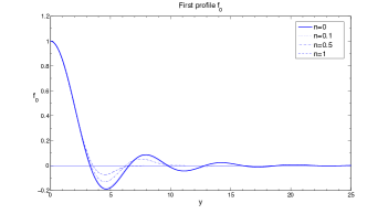
Figure 1. Profiles of the first eigenfunction $f_{0}$ for selected $n$. Obtained by numerical solution of (5.1)–(5.3) in one-dimension $N=1$.

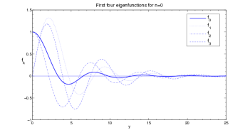
Figure 2. Profiles of the first four eigenfunctions $f_{k}$, $k=0,1,2,3,$ in the case $n=0$. Obtained by numerical solution of (5.4)–(LABEL:fkn0bc2) in one-dimension $N=1$.

Appendix A: Unstable TFE-10 model with an extra backward diffusion term

A.1. Main model and problem setting

Hereafter, we study the global-in-time behaviour of solutions of the tenth-order quasilinear evolution equation of parabolic type, called the unstable TFE-10 (1.8), with the homogeneous diffusion term of backward in time porous medium type, where $n>0$ and $p>n+1$ are given parameters. Equation (1.8) is also (as (1.1)) written for solutions of changing sign, which can occur in the CP and also in some FBPs.

For both the FBP and the CP, the solutions are assumed to satisfy standard free-boundary conditions or boundary conditions at infinity (2.1) at the singularity surface (interface) $\Gamma_{0}[u]$ given in (2.2). For sufficiently smooth interfaces, the condition on the flux now reads

(A.1) $$\lim_{\hbox{dist}(x,\Gamma_{0}[u])\downarrow 0}-{\bf n}\cdot(|u|^{n}\nabla\Delta^{4}u+\nabla|u|^{p-1}u)=0.$$

Then, differentiating the mass $M(t)$ in (2.3) with respect to $t$ and applying the divergence theorem (under natural regularity assumptions on solutions and free boundary), we get

$$\textstyle{J(t):=\frac{{\mathrm{d}}M}{{\mathrm{d}}t}=-\int\limits_{\Gamma_{0}\cap\{t\}}{\bf n}\cdot(|u|^{n}\nabla\Delta^{4}u+\nabla|u|^{p-1}u)\,.}$$

The mass is conserved if $J(t)\equiv 0$, which is assured by the flux condition (A.1). The problem is completed with bounded, smooth, integrable, compactly supported initial data denoted by (2.4).

In the CP for (1.8) in $\mathbb{R}^{N}\times\mathbb{R}_{+}$, one needs to pose bounded compactly supported initial data (2.4) prescribed in $\mathbb{R}^{N}$. Then, under the same zero flux condition at finite interfaces (to be established separately), the mass is preserved.

A.2. Global similarity solutions

We now specify the self-similar solutions of the equation (1.8), which are admitted due to its natural scaling-invariant nature. In the case of the mass being conserved, we have global in time source-type solutions. Using the following scaling in (1.8) $x:=\mu\bar{x}$, $t:=\lambda\bar{t}$, $u:=\nu\bar{u}$, we obtain invariance provided $\mu=\lambda^{\beta}$, $\nu=\lambda^{-\alpha}$, where

(A.2) $$\textstyle{\alpha:=\frac{4}{5p-(n+5)}\quad\hbox{and}\quad\beta:=\frac{p-(n+1)}{2[5p-(n+5)]}.}$$

This suggests considering similarity solutions of the form

(A.3) $$\textstyle{u(x,t):=t^{-\alpha}f(y),\quad\hbox{with}\quad y:=\frac{x}{t^{\beta}}.\quad}$$

Substituting into (1.1) and rearranging terms, we find that the function $f$ solves a quasilinear elliptic equation of the form

(A.4) $$\nabla\cdot\left[|f|^{n}\nabla\Delta^{4}f-\nabla(|f|^{p-1}f)\right]+\beta\,y\cdot\nabla f+\alpha f=0\,.$$

The parameters $\alpha$ and $\beta$ (as given in (A.2)) are linked by the following expressions

$$\textstyle{10\beta-n\alpha=1,\quad 2\beta-\alpha(p-1)=1.}$$

Finally, due to the above relations between $\alpha$ and $\beta$, we find a nonlinear eigenvalue problem of the form

(A.5) $$\framebox{$\textstyle{\nabla\cdot\left[|f|^{n}\nabla\Delta^{4}f-\nabla(|f|^{p-1}f)\right]+\frac{1+\alpha n}{10}\,y\cdot\nabla f+\alpha f=0,\quad f\in C_{0}(\mathbb{R}^{N})\,,}$}$$

where we add to the equation (A.4) a natural assumption that $f$ must be compactly supported (and, of course, sufficiently smooth at the interface, which is an accompanying question to be discussed as well).

Thus, for such degenerate elliptic equations, the functional setting in (A.5) assumes that we are looking for (weak) compactly supported solutions $f(y)$ as certain “nonlinear eigenfunctions” that hopefully occur for special values of nonlinear eigenvalues $\{\alpha_{\gamma}\}_{|\gamma|\geq 0}$. Similar to the previous problem, we intend to justify (formally, at least) that (1.4) holds for the problem (A.5). Moreover, again for this particular situation, in the linear case $n=0$, the condition $f\in C_{0}(\mathbb{R}^{N})$, is replaced by the requirement that the eigenfunctions $\psi_{\beta}(y)$ exhibit typical exponential decay at infinity by using the weighted space (2.5).

Next, using the mass evolution (2.6), in the case $\int f\not=0$, the exponents are calculated giving the first explicit nonlinear eigenvalue:

(A.6) $$\textstyle{-\alpha+\beta N=0\quad\Longrightarrow\quad p_{0}(n)=n+1+\frac{8}{N},\quad\alpha_{0}(n)=\frac{N}{10+Nn}\quad\mbox{and}\quad\beta_{0}(n)=\frac{1}{10+Nn}.}$$

So far, the analysis looks rather similar to the one performed previously for the 10$th$–order equation without the extra diffusion term (1.3). However, the results seem to be quite different. The main difference is that, for (1.3) (rescaled version of (1.1)), we ascertained the branching–asymptotic analysis from the solutions or eigenfunctions of the rescaled poly-harmonic equation (3.4). For (A.5), the solutions will emanate from the solutions of a nonlinear perturbation of the equation (3.4), basically due to the extra diffusion term.

It was obtained in [9] that, for the fourth–order unstable TFE4,

(A.7) $$u_{t}=-\nabla\cdot(|u|^{n}\nabla\Delta u)-\Delta(|u|^{p-1}u)\quad\mbox{in}\quad\mathbb{R}^{N}\times\mathbb{R}_{+}\,,$$

there are continuous families of solutions of global similarity solutions when the exponent $p$ is the critical exponent $\textstyle{p=p_{0}=n+1+\frac{4}{N}.}$ Moreover, the authors also showed that in the particular case when $p\neq p_{0}$ the families of similarity solutions become countable.

Let us briefly comment on that. Namely, in 1D, the main reason in the critical case $p=p_{0}$ to admit wider (a continuum) family of solutions is that the corresponding rescaled ODE admits integration once and reduces to a third-order ODE, which makes a shooting procedure underdetermined: two parameters to satisfy a single symmetry conditions at the origin. For $p\neq p_{0}$, the ODE is truly fourth-order, and the shooting is well-posed: two parameters and two symmetry conditions.

A similar situation occur the above unstable TFE-10: for $p=p_{0}$ there exists symmetry reduction and the ODE in 1D becomes of ninth order. This analysis could be extended to our 10$th$–order equation Therefore, (1.8) admits continuous families of global similarity solutions if $p=p_{0}$ given in (A.6) and, also, for $p\neq p_{0}$ we will have a countable family of solutions for the unstable TFE–10 (1.8).

For equations in $\mathbb{R}^{N}$, a similar result holds true in the radial setting, where we deal with ODEs again. Non-radial patterns are entirely unknown and, honestly, we do not have any clue how and by what tools these can be detected (numerics are expected also to be extremely difficult).

Therefore (in the in ODE setting), performing a similar branching analysis, as the one done in the previous section for the TFE–10 (1.1), we obtain that (1.8) possesses a countable set of eigenfunction/value pairs $\{f_{k},\,\alpha_{k}\}_{k\geq 0}$ (1.4) such that the solutions of the equation (A.5) emanate from the solutions of the rescaled version Cahn–Hilliard equation type

(A.8) $$u_{t}=\Delta^{5}u-\Delta(|u|^{p-1}u)\quad\mbox{in}\quad\mathbb{R}^{N}\times\mathbb{R}_{+},\,,$$

at $n=0$. In other words, the solutions of the equation

(A.9) $$\textstyle{\Delta^{5}f-\Delta(|f|^{p-1}f)+\frac{1}{10}\,y\cdot\nabla f+\alpha f=0,\quad f\in H^{10}_{\rho}(\mathbb{R}^{N})\,,}$$

for certain values of the parameter $\alpha$, which will provide us with that countable family of solutions emanating form the solutions of (A.9) at $n=0$. One can easily see that (A.9) is a nonlinear perturbation of the rescaled equation (3.4). Moreover, to detect a deeper connection with linear eigenfunctions, a further homotopy deformation analysis should be performed by passing $p\to 1^{+}$ leading to the linear eigenvalue problem

(A.10) $$\textstyle{\Delta^{5}f-\Delta f+\frac{1}{10}\,y\cdot\nabla f+\alpha f=0,\quad f\in H^{10}_{\rho}(\mathbb{R}^{N})\,,}$$

which admits a clear study similar to [7]. It is important that we can describe the whole complete family of eigenfunctions of (A.10) including all the non-radial ones.

Thus, it turns out that the solutions of the equation (1.8) can emanate from a nonlinear perturbed version of the eigenfunctions for the equation (3.4) via two-parametric homotopy deformation to a linear eigenvalue problem. This, at least, very formally explains the origin of countablity of nonlinear eigenfunctions family of those TFEs-10.

References

- [1] Álvarez-Caudevilla, P., Evans, J.D. and Galaktionov, V.A, The Cauchy problem for a tenth-order thin film equation II. Oscillatory source-type solution, in preparation.
- [2] Álvarez-Caudevilla, P. and Galaktionov, V.A,, Local bifurcation-branching analysis of global and “blow-up” patterns for a fourth-order thin film equation, Nonlinear Differ. Equat. Appl., 18 (2011), 483–537 .
- [3] Greer, J. B. and Bertozzi, A. L. , Traveling wave solutions of fourth order PDEs for image processing, SIAM J. Math. Anal. (electronic), 36 (2004), 38–68.
- [4] Birman, M.S. and Solomjak, M.Z., Spectral Theory of Self-Adjoint Operators in Hilbert Spaces, D. Reidel, Dordecht/Tokyo (1987).
- [5] Chaves, M. and Galaktionov, V.A., On source-type solutions and the Cauchy problem for a doubly degenerate sixth-order thin film equation. I. Local oscillatory properties, Nonlinear Anal., 72 (2010), 4030- 4048.
- [6] Deimling, K., Nonlinear Functional Analysis, Springer-Verlag, Berlin/Tokyo, 1985.
- [7] Egorov, Y.V., Galaktionov, V.A., Kondratiev, V.A. and Pohozaev, S.I., Global solutions of higher-order semilinear parabolic equations in the supercritical range, Adv. Differ. Equat., 9 (2004), 1009–1038.
- [8] Evans, J.D. and Galaktionov, V.A and King, J.R., Blow-up similarity solutions of the fourth-order unstable thin film equation, Euro. J. Appl. Math., 18 (2007), 195–231.
- [9] Evans, J.D. and Galaktionov, V.A and King, J.R., Source-type solutions of the fourth-order unstable thin film equation, Euro. J. Appl. Math., 18 (2007), 273–321.
- [10] Evans, J.D. and Galaktionov, V.A and King, J.R., Unstable sixth-order thin film equation I. Blow-up similarity solutions, Nonlinearity, 20 (2007), 1799–1841.
- [11] Evans, J.D. and Galaktionov, V.A and King, J.R., Unstable sixth-order thin film equation II. Global similarity patterns, Nonlinearity, 20 (2007), 1843–1881.
- [12] Galaktionov, V.A., Geometric Sturmian Theory of Nonlinear Parabolic Equations and Applications, ChapmanHall/CRC, Boca Raton, Florida, 2004.
- [13] Galaktionov, V.A., Countable branching of similarity solutions of higher-order porous medium type equations, Adv. Differ. Equat., 13 (2008), 641–680.
- [14] Galaktionov, V.A., Very singular solutions for thin film equations with absorption, Studies Appl. Math., 126 (2011), 103–143 (arXiv:0109.3982).
- [15] Galaktionov, V.A., Mitidieri, E. and Pohozaev, S.I., Variational approach to complicated similarity solutions of higher-order nonlinear evolution equations of parabolic, hyperbolic, and nonlinear dispersion types, In: Sobolev Spaces in Mathematics. II, Appl. Anal. and Part. Differ. Equat., Series: Int. Math. Ser., Vol. 9, V. Maz’ya Ed., Springer, New York, 2009 (an earlier preprint: arXiv:0902.1425).
- [16] Galaktionov, V.A., Mitidieri, E. and Pohozaev, S.I., Variational approach to complicated similarity solutions of higher-order nonlinear PDEs. II, Nonl. Anal.: RWA, 12 (2011), 2435–2466 (arXiv:1103.2643).
- [17] Guidotti, P. and Longo, K., Well–posedness for a class fourth–order diffusions for image processing, Nonl. Diff. Equ. Appl. (NoDEA), 18 (2011), 407–425.
- [18] Krasnosel’skii, M.A. and Zabreiko, P.P., Geometrical Methods of Nonlinear Analysis, Springer-Verlag, Berlin/Tokio, 1984.
- [19] Liu, C., A sixth order degenerate equation with the higher order –Laplacian operator, Mathematica Slovaca, 60, no. 6 (2010), 847–864.
- [20] Liu, C., Qualitative properties for a sixth–order thin film equation, Mathematical Modelling and Analysis, 15 (2010), 457–471.
- [21] Liu, X., Qu, C., Existence and blow-up of weak solutions for a sixth-order equation related to thin solid films, Nonlinear Anal. Real World Appl., 11 (2010), 4214–4222.
- [22] Vainberg, M.A. and Trenogin, V.A., Theory of Branching of Solutions of Non-Linear Equations, Noordhoff Int. Publ., Leiden, 1974.