A. Stern’s analysis of the nodal sets of some families of spherical harmonics revisited

Abstract

In this paper, we revisit the analyses of Antonie Stern (1925) and Hans Lewy (1977) devoted to the construction of spherical harmonics with two or three nodal domains. Our method yields sharp quantitative results and a better understanding of the occurrence of bifurcations in the families of nodal sets.This paper is a natural continuation of our critical reading of A. Stern’s results for Dirichlet eigenfunctions in the square, see arXiv:14026054. 35B05 35P20 58J50

1 Introduction

Let $D$ be a regular bounded domain in ${\mathbb{R}}^{n}$. Let $\Delta$ be the non-positive Laplacian with Dirichlet or Neumann boundary conditions. We arrange the eigenvalues $(\lambda_{j})_{j\in\mathbb{N}^{*}}$ of $-\Delta$ in increasing order,

$$\lambda_{1}<\lambda_{2}\leq\lambda_{3}\leq\cdots.$$

Courant’s 1923 celebrated nodal domain theorem Cou , (CH, , p. 452) states that an eigenfunction associated with the $n$-th eigenvalue $\lambda_{n}$, has at most $n$ nodal domains. On the other hand, an eigenfunction associated with $\lambda_{n}$, has at least two nodal domains when $n\geq 2$. The question remained of an eventual lower bound for the number of nodal domains of an $n$-th eigenfunction, as in the Sturm-Liouville theory. Antonie Stern’s 1924 thesis St , written under the supervision of Richard Courant, contains the following three results which provide a negative answer to this question.

Theorem 1.1

Let $D$ be the unit square in ${\mathbb{R}}^{2}$, and $\Delta$ the non-positive Laplacian with Dirichlet boundary conditions. Then, for any integer $m$, there exists an eigenfunction $u$ of $-\Delta$, associated with the eigenvalue $(4m^{2}+1)\pi^{2}$, whose nodal set inside the square consists of a single simple closed curve. As a consequence, $u$ has exactly two nodal domains.

Theorem 1.2

Let $\mathbb{S}^{2}$ be the unit sphere in ${\mathbb{R}}^{3}$, and $\Delta$ the non-positive spherical Laplacian. For any odd integer $\ell$, there exists a spherical harmonic of degree $\ell$, whose nodal set consists of a single simple closed curve. As a consequence, $u$ has exactly two nodal domains.

Theorem 1.3

Let $\mathbb{S}^{2}$ be the unit sphere in ${\mathbb{R}}^{3}$, and $\Delta$ the non-positive spherical Laplacian. For any even integer $\ell\geq 2$, there exists a spherical harmonic of degree $\ell$, whose nodal set consists of two disjoint simple closed curves. As a consequence, $u$ has exactly three nodal domains.

Recall that the eigenfunctions of the spherical Laplacian are the spherical harmonics, i.e.  the restriction to the sphere $\mathbb{S}^{2}$ of the harmonic homogeneous polynomials in ${\mathbb{R}}^{3}$.

Theorem 1.1 is stated without proof in (CH, , p. 455), with a reference to Stern’s thesis St , and illustrated by two figures taken from St . Theorems  1.2 and 1.3 are apparently not mentioned in CH . They were rediscovered in 1977 by Hans Lewy (Lew, , Theorems 1 and 2), without any reference to A. Stern. In the introduction of his paper, Lewy also explains why a spherical harmonic of positive even degree has at least three nodal domains.

In St1 , we provide extracts from Stern’s thesis, with annotations and highlighting of the main assertions and ideas. Stern’s thesis is rather discursive. The main results are not stated in theorem form, as above. They appear in the course of the thesis, for example in the following citations (see Appendix B for a translation into English) (St1, , tags E1, K1, K2):

[E1] …es läßt sich beispielweise leicht zeigen, daß auf der Kugel bei jedem Eigenwert die Gebietszahlen $2$ oder $3$ auftreten, und daß bei Ordnung nach wachsenden Eigenwerten auch beim Quadrat die Gebietszahl $2$ immer wieder vorkommt.

[K1] Zunächst wollen wir zeigen, daß es zu jedem Eigenwert Eigenfunktionen gibt, deren Nullinien die Kugelfläche nur in zwei oder drei Gebiete teilen. ……Die Gebietszahl zwei tritt somit bei allen Eigenwerten $\lambda_{n}=(2r+1)(2r+2)\,~{}r=1,2,\cdots$ auf ;
[K2] ebenso wollen wir jetzt zeigen, daß die Gebietszahl drei bei allen Eigenwerten $\lambda_{n}=2r(2r+1),~{}r=1,2,\cdots$ immer wieder vorkommt.

Stern’s proofs are far from being complete, but she provides nice geometric arguments (St1, , tags I1-I3), and figures.

[I1] Legen wir die beiden Knotenliniensysteme übereinander und schraffieren wir die Gebiete, in denen beide Funktionen gleiches Verzeichen haben, so kann die Knotenlinie der Kugelfunktion

$$P^{2r+1}_{2r+1}(\cos\vartheta)\cos(2r+1)\varphi+\mu P_{2r+1}(\cos\vartheta)\,,\quad\mu>0$$

nur in der nichtschraffierten Gebieten verlaufen
[I3]  und zwar für hinreichend kleine $\mu$ in beliebiger Nachbarschaft der Knotenlinien von

$$P^{2r+1}_{2r+1}(\cos\vartheta)\cos(2r+1)\varphi,$$

d. h. der $2r+1$ Meridiane, da sich bei stetiger Änderung von $\mu$ das Knotenliniensystem stetig ändert ….
[I2] Da die Knotenlinie ferner durch die $2(2r+1)^{2}$ Schnittpunkte der Nullinien der beiden obenstehenden Kugelfunktionen gehen muß …

Sketch of Stern’s proofs, and comparison with Lewy’s paper Lew . A. Stern starts from an eigenfunction $u$, whose nodal set can be completely described. In the case of the unit square, this function $u$ is chosen to be $\sin(2m\pi x)\,\sin(\pi y)+\sin(\pi x)\,\sin(2m\pi y)$. In the case of the sphere, it is chosen to be the restriction to the sphere of the homogeneous harmonic polynomial $W(x,y,z)=\Im(x+iy)^{\ell}$. A. Stern then perturbs the eigenfunction $u$ by some eigenfunction $v$ (in the same eigenspace), looking at the family $u^{\mu}=u+\mu v$ for $\mu$ small. The function $v$ is chosen to be $\sin(\pi x)\,\sin(2m\pi y)$ in the case of the square, and a spherical harmonic whose nodal sets mainly contains latitude circles (parallels) in the case of the sphere.

The main observation made by Stern is that for $\mu>0$, the nodal set $N(u^{\mu})$ satisfies

$${\cal N}\subset N(u^{\mu})\subset{\cal N}\cup\{u\,v<0\},$$

where ${\cal N}=N(u)\cap N(v)$ is the set of zeros common to $u$ and $v$. In the case of the square, the connected components of the set $\{u\,v\neq 0\}$ are small squares, whose vertices belong to ${\cal N}$. In the case of the sphere, they are square-like domains with vertices in ${\cal N}$, and triangle-like domains one of whose vertices is the north or south pole, and the others belong to ${\cal N}$. In both cases, the domains form a kind of grey/white checkerboard (the connected open sets on which $u\,v$ is positive/negative) on the unit square or on the sphere. The above inclusions say that the nodal set $N(u^{\mu})$ contains ${\cal N}$, and has to avoid the grey squares, see (St1, , tags I1, I2). A. Stern concludes, without proof, by saying that the nodal set $N(u^{\mu})$ deforms continuously, and remains close to the nodal set $N(u)$ when $\mu$ is small, (St1, , tag I3).

To prove Theorems 1.2 and 1.3, Lewy Lew analytically determines how the nodal sets deform under small perturbations, first locally, and then globally. Continuity arguments were later explored in LeyD .

For a given degree $\ell$, A. Stern St and H. Lewy Lew give examples of a spherical harmonic $h_{o}$ whose nodal set is a simple closed regular curve, when the degree is odd; and of a spherical harmonic $h_{e}$ whose nodal set consists of two disjoint simple closed regular curves, when the degree is even.

When the degree $\ell$ is odd, Stern and Lewy start from the spherical harmonic $W$, whose expression in spherical coordinates is given by $w(\vartheta,\varphi)=\sin^{\ell}(\vartheta)\,\sin(\ell\varphi)$, and consider the family $W+\mu F$, where $F$ is a spherical harmonic of degree $\ell$. Lewy (Lew, , Theorem 1) only requires that $F(p_{+})>0$, where $p_{+}$ is the north pole. Stern (see the proof of Proposition 3.3) chooses $F$ to be the zonal spherical harmonic given by $P_{\ell}(\cos\vartheta)$ in spherical coordinates. As we shall see, for $\mu$ small enough, $0$ is a regular value of $W+\mu F$, and the nodal set $N(W+\mu F)$ is connected. As a consequence, one has two-parameter families of spherical harmonics whose nodal sets are simple closed regular curves, and hence with two nodal domains.

When the degree $\ell\geq 2$ is even, Stern and Lewy use different functions. Stern starts from the spherical harmonic $W$, and perturbs it by the spherical harmonic $V_{\alpha}$ whose expression in spherical coordinates is given by $v_{\alpha}(\vartheta,\varphi)=P_{\ell}^{1}(\cos\vartheta)\,\sin(\varphi-\alpha)$. As we shall see, for $\mu$ small enough, $0$ is a regular value of $W+\mu V_{\alpha}$ (see the proof of Proposition 4.3), and the nodal set $N(W+\mu V_{\alpha})$ has two connected components. This construction gives us a three-parameter family of spherical harmonics of even degree $\ell$, admitting $0$ as a regular value, and whose nodal sets have two connected components, and hence with three nodal domains. Lewy (Lew, , Theorem 2) first constructs a spherical harmonic $F$ of the form $F(x,y,z)=x\,y\,F_{1}(x,y,z)$, where the function $F_{1}$ only depends on the distance to the north pole $p_{+}$. The nodal set $N(F)$ consists of two orthogonal great circles through the poles $p_{\pm}$, and $(\ell-2)$ latitude circles. The nodal set $N(F)$ has $4(\ell-2)+2$ singular points which are double crossings. Lewy then constructs a spherical harmonic $G$, of degree $\ell$, with ad hoc signs at the singular points of $N(F)$, so that $F+\mu G$ desingularizes $N(F)$ when $\mu$ is small enough. He then shows that, for $\mu$ small enough, $0$ is a regular value of $F+\mu G$, and that the nodal set $N(F+\mu G)$ has two connected components. This construction yields a two-parameter family of such spherical harmonics.

As a matter of fact, one can prove that the set of spherical harmonics of odd degree $\ell$ (resp. of even degree $\ell$), which admit $0$ as a regular value, and whose nodal set is connected (resp. whose nodal set has two connected components), is an open set in the vector space ${\cal H}_{\ell}$ of spherical harmonics of degree $\ell$. This is a consequence of the inverse function theorem and of the existence of the above examples.

A. Stern’s proofs lack important details, while Lewy’s paper is written in a rather condensed analytical style. In BeHe , we gave a complete geometric proof of Theorem 1.1. In this paper, we give a complete geometric proof of quantitative versions of Theorems 1.2 and  1.3 (see Propositions 3.3 and 4.3 respectively). In each case, we start from Stern’s geometric ideas, and we make a precise analysis of the possible local nodal patterns in the square-like and triangle-like domains. More precisely, we supplement Stern’s ideas with,

1. an analysis of the critical zeros (a critical zero of a function $f$ is a point at which both $f$ and its differential $df$ vanish), showing in particular that $u^{\mu}$ does not have any critical zero when $\mu\neq 0$ is small enough (Lemmas 3.1 and 4.1);

2. separation lemmas (Lemmas 3.2 and 4.2) to exclude certain local nodal patterns (in our proof, they replace Lewy’s continuity arguments);

3. an energy argument to show that a connected component of the set $\{u\,v\neq 0\}$ cannot contain a simple closed nodal curve of $u^{\mu}$, see Properties 3.2.3 (iii) and Properties 4.2.4 (vii);

4. classical properties of nodal sets of eigenfunctions, as summarized in (BeHe, , Section 5.2).

Our proofs yield sharp quantitative results, Propositions 3.3 and 4.3, and a better understanding of the occurrence of bifurcations in the families of nodal sets, Lemmas 3.1 and 4.1. We in particular show that there exists some positive $\mu_{c}$ such that, for $0<\mu<\mu_{c}$, the nodal set of $u^{\mu}$ is a regular $1$-dimensional submanifold of the sphere, while the nodal set of $u^{\mu_{c}}$ has self-intersections.

As far as Courant’s theorem is concerned, another natural question is whether Courant’s upper bound is sharp. For $2$-dimensional Euclidean domains with Dirichlet boundary condition, using the Faber-Krahn inequality in an essential way, Åke Pleijel Pl proved that the number of nodal domains of an $n$-th eigenfunction is asymptotically less than $0.7\,n~{}$ (more precisely, less than $\gamma(2)\,n$, with $\gamma(2):=4\pi/\lambda(Disk_{1})$, where $\lambda(Disk_{1})$ is the lowest eigenvalue of the Dirichlet Laplacian in the disk of area $1$). As a corollary, one can conclude that Courant’s theorem is sharp for finitely many eigenvalues only. Pleijel’s result was later generalized to any compact Riemannian manifold $M$ (with Dirichlet boundary condition if $\partial M\neq\emptyset$), with a universal constant $\gamma(n)<1$ depending only on the dimension $n$ of $M$, see Pe ; BeMe . The case of the Neumann boundary condition was also considered by Pleijel Pl for the square, and recently revisited in Pol (in a more general setting: dimension 2, piecewise real analytic boundary), and in HP . Starting in 2009, there has been a renewed interest for Courant’s theorem in the context of minimal partitions, and the investigation of the cases in which Courant’s theorem is sharp HHOT ; HHOT1 , see Section 5. These developments motivated BeHe and motivate the present paper.

The paper is organized as follows. In Section 2 we recall some properties of spherical harmonics and Legendre functions. In Sections 3 and 4, we give detailed geometric proofs of Stern’s second and third theorems for the sphere, with quantitative statements (Propositions 3.3 and 4.3). In Section 5, we recall the state of the art on the question of Courant sharpness for the sphere. In Appendix A, we provide some numerical computations of nodal sets of spherical harmonics. In Appendix B, we provide a translation into English of the citations from Stern’s thesis.

2 Preliminaries

2.1 Spherical harmonics

Denote by $\mathbb{S}^{2}:=\{(x,y,z)\in{\mathbb{R}}^{3}~{}|~{}x^{2}+y^{2}+z^{2}=1\}$ the round $2$-sphere. Given an integer $\ell\in{\mathbb{N}}$, we call ${\cal H}_{\ell}$ the vector space of spherical harmonics of degree $\ell$ i.e., the restriction to the sphere of the harmonic homogeneous polynomials in $3$ variables in ${\mathbb{R}}^{3}$. This is the eigenspace of $-\Delta$ on $\mathbb{S}^{2}$, associated with the eigenvalue $\ell(\ell+1)$. It has dimension $2\ell+1$. Given a spherical harmonic $h(\xi,\eta,\zeta)$ of degree $\ell$, with $(\xi,\eta,\zeta)\in\mathbb{S}^{2}$, one can recover the harmonic homogeneous polynomial $H$ it comes from as follows. Let $r=(x^{2}+y^{2}+z^{2})^{1/2}$. Then,

$$H(x,y,z)=r^{\ell}\,h(xr^{-1},yr^{-1},zr^{-1})\,.$$ (2.1)

For simplicity, we shall henceforth identify the spherical harmonic $h$ and the polynomial $H$.

The space ${\cal H}_{0}$ is $1$-dimensional, associated with the eigenvalue $0$. The space ${\cal H}_{1}$ has dimension $3$. It is associated with the eigenvalue $2$, and is generated by the coordinate functions $x,y$ and $z$ which have exactly two nodal domains. The space ${\cal H}_{2}$ has dimension $5$. It is associated with the eigenvalue $6$, and is generated by the polynomials $yz,xz,xy,2z^{2}-x^{2}-y^{2}$ and $x^{2}-z^{2}$. It is easy to check that for $\mu>0$, small enough, the spherical harmonic $xy+\mu\,(2z^{2}-x^{2}-y^{2})$ has exactly three nodal domains: the nodal set of the spherical harmonic consists of two simple closed curves given by the intersection of the sphere with a right cylinder over a hyperbola in the $\{x,y\}$-plane. Following A. Stern, we shall later on consider a perturbation of the degree $\ell$ spherical harmonic $\Im(x+iy)^{\ell}$.

We denote the north and south poles of $\mathbb{S}^{2}$ respectively by $p_{+}=(0,0,1)$ and $p_{-}=(0,0,-1)$.

By abuse of language, we shall call spherical coordinates on the sphere $\mathbb{S}^{2}$, the map

$$\left\{\begin{aligned} &E:[0,\pi]\times{\mathbb{R}}\to\mathbb{S}^{2}\,,\\ &E(\vartheta,\varphi)=(\sin\vartheta\,\cos\varphi,\sin\vartheta\,\sin\varphi,\cos\vartheta)\,,\end{aligned}\right.$$ (2.2)

where $\vartheta$ is the co-latitude, and $\varphi$ the longitude.
The map $E$ is a diffeomorphism from $(0,\pi)\times(\varphi_{0},2\pi+\varphi_{0})$ onto $\mathbb{S}^{2}\setminus M_{\varphi_{0}}$, where $M_{\varphi_{0}}=E([0,\pi],\varphi_{0})$ is the meridian from $p_{+}$ to $p_{-}$ with longitude $\varphi_{0}$. To cover $\mathbb{S}^{2}\setminus\{p_{\pm}\}$, we will work in $(0,\pi)\times{\mathbb{R}}_{2\pi}$ i.e., modulo $2\pi$ in the $\varphi$ variable ($\mathbb{R}_{2\pi}=\mathbb{R}/(2\pi\mathbb{Z})$).

The map $E$ can be viewed as the polar coordinates in the exponential map $exp_{p_{+}}$, which sends the disk $D(0,\pi)$, with center $0$ and radius $\pi$ in $T_{p_{+}}\mathbb{S}^{2}$ (the tangent plane to the sphere at $p_{+}$), onto $\mathbb{S}^{2}\setminus\{p_{-}\}$ diffeomorphically. The variable $\vartheta$ is the distance to the north pole.

In the spherical coordinates, the antipodal map is given by $(\vartheta,\varphi)\to(\pi-\vartheta,\pi+\varphi)$.

In the sequel, we will illustrate the proofs by figures representing the nodal patterns viewed through the exponential map i.e., in the disk $D(0,\pi)$. In the figures, the outer circle always represents the circle of radius $\pi$ i.e., the cut-locus of the north pole.

Using the spherical coordinates, the spherical harmonics can be described in terms of Legendre functions and polynomials. In the next section, we fix some notation, and recall useful properties of Legendre functions and polynomials.

2.2 Legendre functions and polynomials

The $(2\ell+1)$-dimensional vector space ${\cal H}_{\ell}$ of spherical harmonics of degree $\ell$ admits the basis,

$$P_{\ell}(\cos\vartheta),~{}P_{\ell}^{m}(\cos\vartheta)\,\cos(m\varphi),~{}P_{\ell}^{m}(\cos\vartheta)\,\sin(m\varphi)\,,$$ (2.3)

where $m$ is an integer $1\leq m\leq\ell$, $P_{\ell}$ the Legendre polynomial of degree $\ell$, and $P_{\ell}^{m}$ the Legendre functions. We use the notation and the normalizations of MOS .

For $0\leq m\leq\ell$, the Legendre function $P_{\ell}^{m}$ satisfies the differential equation,

$$\left((1-t^{2})P^{\prime}(t)\right)^{\prime}+\left(\ell(\ell+1)-\frac{m^{2}}{1-t^{2}}\right)P(t)=0\,.$$ (2.4)

When $m$ is $0$, $P_{\ell}^{m}=P_{\ell}$ . Furthermore, the following properties hold.

1. Identities.

   $$P_{\ell}(t)=\frac{1}{2^{\ell}\ell!}\left(\frac{d}{dt}\right)^{\ell}(t^{2}-1)^{\ell}\,,$$ (2.5)

   $$P_{\ell}^{m}(t)=(-1)^{m}(1-t^{2})^{m/2}\left(\frac{d}{dt}\right)^{m}P_{\ell}(t)\,,$$ (2.6)

   and

   $$(1-t^{2})\,P_{\ell}^{\prime}(t)=\ell\,P_{\ell-1}(t)-\ell\,t\,P_{\ell}(t)\,.$$ (2.7)

   In particular, $P_{\ell}^{\ell}(\cos\vartheta)=C_{\ell}\sin^{\ell}(\vartheta)\,$, where $C_{\ell}$ is a constant.

2. The polynomial $P_{\ell}$ has degree $\ell$, the same parity as the integer $\ell$, and satisfies

   $$P_{\ell}(1)=1\,,\,P_{\ell}(-1)=(-1)^{\ell}\,,$$ (2.8)

   and

   $$\sup_{[-1,1]}|P_{\ell}(t)|=1\,.$$ (2.9)

3. The polynomial $P_{\ell}(t)$ has $\ell$ simple roots $t_{j}(\ell)$ ($j=1,\cdots,\ell$) in the interval $(-1,1)$, enumerated in decreasing order. We write these roots as $t_{j}(\ell)=\cos(\vartheta_{j}(\ell))$, with

   $$0<\vartheta_{1}(\ell)<\vartheta_{2}(\ell)<\cdots<\vartheta_{\ell-1}(\ell)<\vartheta_{\ell}(\ell)<\pi\,.$$ (2.10)

   The derivative $P^{\prime}_{\ell}(t)$ has $(\ell-1)$ simple roots which we write as $\cos\left(\vartheta^{\prime}_{j}(\ell)\right)$. They satisfy

   $$0<\vartheta_{1}(\ell)<\vartheta^{\prime}_{1}(\ell)<\vartheta_{2}(\ell)<\cdots<\vartheta_{\ell-1}(\ell)<\vartheta^{\prime}_{\ell-1}(\ell)<\vartheta_{\ell}(\ell)<\pi\,.$$ (2.11)

   Note that the values $\vartheta_{j}(\ell)$ and $\vartheta^{\prime}_{j}(\ell)$ are symmetrical with respect to $\frac{\pi}{2}$. As a consequence, for $\ell$ odd, $P_{\ell}(0)=0$ and $P^{\prime}_{\ell}(0)\neq 0$, and for $\ell$ even, $P_{\ell}(0)\neq 0$ and $P^{\prime}_{\ell}(0)=0$.

4. The polynomials $P_{\ell}$ and $P_{\ell-1}$ have no common zero. More precisely, the zeros of $P_{\ell}$ and $P_{\ell-1}$ are intertwined:

   $$0<\vartheta_{1}(\ell)<\vartheta_{1}(\ell-1)<\vartheta_{2}(\ell)<\cdots<\vartheta_{\ell-1}(\ell)<\vartheta_{\ell-1}(\ell-1)<\vartheta_{\ell}(\ell)<\pi\,.$$ (2.12)

5. For the zeros of $P_{\ell}$, one has the inequalities,

   $$\frac{2j-1}{2\ell+1}\pi<\vartheta_{j}(\ell)<\frac{2j}{2\ell+1}\pi\,,\,\mbox{ for }j=1,\cdots,\ell\,.$$ (2.13)

6. Call $p_{j}(\ell),~{}1\leq j\leq[\frac{\ell}{2}]$, the local maxima of $|P_{\ell}(t)|$, when $t$ decreases from $1$ to $0$. Then,

   $$0<p_{[\frac{\ell}{2}]}(\ell)<\cdots<p_{2}(\ell)<p_{1}(\ell)<1\,.$$ (2.14)

   Here $[\cdot]$ denotes the integer part.

7. For the derivative of the Legendre polynomial $P_{\ell}(t)$, one has the inequality,

   $$|P^{\prime}_{\ell}(t)|\leq\frac{\ell(\ell+1)}{2}\text{~{}~{}for~{}~{}}-1\leq t\leq 1\,,$$ (2.15)

   where the equality is achieved for $\ell=0,1$ and when $\ell\geq 2$, for $t=\pm 1$.

For these properties, we refer to (MOS, , Chapters IV and V) and to Sz . In particular, Properties (v)-(vii) can be found in Sz , resp. under Theorems 6.21.2, 7.3.1, and Inequality (7.33.8).

Remarks. (i) Using (2.7), one can prove that for $1\leq j\leq\ell-1$,

$$\vartheta_{j}(\ell)<\vartheta_{j}(\ell-1)<\vartheta^{\prime}_{j}(\ell)\,.$$ (2.16)

(ii) One can relate the asymptotic behavior of $\vartheta_{1}(\ell)$ as $\ell\rightarrow+\infty$, to the first zero $j_{0,1}$ of the zero-th Bessel function $J_{0}$, (Sz, , Theorem 8.1.2),

$$\vartheta_{1}(\ell)\sim{j_{0,1}}/\ell\,.$$ (2.17)

(iii) One can also relate the asymptotic behavior of $p_{1}(\ell)$ as $\ell\rightarrow+\infty$, to the first zero $j_{1,1}$ of the Bessel function $J_{1}=-J^{\prime}_{0}$,

$$p_{1}(\ell)\sim-J_{0}(j_{1,1})\,.$$ (2.18)

3 Stern’s first theorem: odd case

The purpose of this section is to prove Theorem 1.2. As a matter of fact, we shall prove a more quantitative result, Proposition 3.2.3, which implies the theorem. We use Stern’s ideas sketched in the introduction.

Fix an integer $\ell\in{\mathbb{N}}$, without any parity assumption for the time being. We work in the spherical coordinates (2.2), with $(\vartheta,\varphi)\in[0,\pi]\times{\mathbb{R}}_{2\pi}$.

3.1 Notation

Up to scaling, there is a unique spherical harmonic $Z_{\ell}$, of degree $\ell$, which is invariant under the rotations about the $z$-axis. Viewed in the spherical coordinates, this zonal spherical harmonic is given by $P_{\ell}(\cos\vartheta)$. Let $\vartheta_{1}(\ell)<\vartheta_{2}(\ell)<\cdots<\vartheta_{\ell}(\ell)$ be the zeros of the function $\vartheta\to P_{\ell}(\cos\vartheta)$ in the interval $(0,\pi)$, see Properties 2.2 (iii). The nodal set of the spherical harmonic $Z_{\ell}$, denoted $N(Z_{\ell})$, consists of precisely $\ell$ latitude circles (parallels),

$$L_{i}:=\{(\vartheta,\varphi)~{}|~{}\vartheta=\vartheta_{i}(\ell)\}\,,~{}1\leq i\leq\ell\,.$$

They determine sectors on the sphere,

$${\cal L}_{i}:=\{(\vartheta,\varphi)~{}|~{}\vartheta_{i}(\ell)<\vartheta<\vartheta_{i+1}(\ell)\}\,,~{}0\leq i\leq\ell\,,$$

where $\vartheta_{0}(\ell)=0$ and $\vartheta_{\ell+1}(\ell)=\pi$. In the sector ${\cal L}_{i}$, the function $Z_{\ell}$ has the sign of $(-1)^{i}\,$.

Call $W_{\ell}$ the spherical harmonic of degree $\ell$ obtained by restricting the harmonic homogeneous polynomial $\Im(x+iy)^{\ell}$ to the sphere. Viewed in spherical coordinates, this spherical harmonic is given by $\sin^{\ell}(\vartheta)\,\sin(\ell\varphi)$. Its nodal set $N(W_{\ell})$ consists of $\ell$ great circles of $\mathbb{S}^{2}$ i.e., of $2\ell$ meridians,

$$M_{j}=\{(\vartheta,\varphi)~{}|~{}\varphi=j\frac{\pi}{\ell}\}\,,~{}0\leq j\leq 2\ell-1\,.$$

They determine sectors on the sphere,

$${\cal M}_{j}=\{(\vartheta,\varphi)~{}|~{}j\frac{\pi}{\ell}<\varphi<(j+1)\frac{\pi}{\ell}\}\,~{}0\leq j\leq 2\ell-1\,.$$

In the sector ${\cal M}_{j}$ the function $W_{\ell}$ has the sign of $(-1)^{j}$.

Note that these meridians meet at the north and south poles $p_{\pm}$ which are the only singular points of the nodal set $N(W_{\ell})\,$.

The intersection

$${\cal N}=N(Z_{\ell})\cap N(W_{\ell})$$

is the finite set of zeros common to $Z_{\ell}$ and $W_{\ell}$.

We call $q_{i,j}$ the intersection point of $L_{i}$ with $M_{j}\,$, $1\leq i\leq\ell\,$, $0\leq j\leq 2\ell-1\,$, so that

$${\cal N}=\{q_{i,j},~{}1\leq i\leq\ell,~{}0\leq j\leq 2\ell-1\}\,.$$

For $0\leq i\leq\ell$ and $0\leq j\leq 2\ell-1$, we introduce the sets ${\cal Q}_{i,j}={\cal L}_{i}\cap{\cal M}_{j}$, which are the connected components of the open set $\{Z_{\ell}\,W_{\ell}\not=0\}$. In ${\cal Q}_{i,j}$ the sign of the function $Z_{\ell}\,W_{\ell}$ is $(-1)^{i+j}\,$.

The sets ${\cal Q}_{i,j}$ form a grid patterns over the sphere, and following the idea of A. Stern, they can be colored according to the sign of the function $Z_{\ell}\,W_{\ell}$ thus forming a checkerboard.

Finally, for $0\leq j\leq 2\ell-1\,$, we introduce the meridian $B_{j}$,

$$B_{j}=\{(\vartheta,\varphi)~{}|~{}\varphi=(j+\frac{1}{2})\frac{\pi}{\ell}\}\,,$$ (3.1)

which bisects the sector ${\cal M}_{j}$.

Figure 3.1 displays the latitude circles and the meridians viewed through the exponential map at the north pole $p_{+}$, in the cases $\ell=3$ and $\ell=4$. The common zeros of $W_{\ell}$ and $Z_{\ell}$ are the big dots. The coloring white/grey illustrates the sign of $Z_{\ell}\,W_{\ell}$. The outer circle is mapped to the south pole by the exponential map.

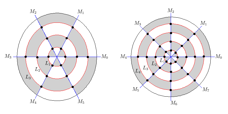
Figure 3.1: Checkerboards in the cases $\ell=3$, and $\ell=4$

3.2 The family $H^{\mu,\ell}$

Following Stern St , we consider the one-parameter family of spherical harmonics,

$$H^{\mu,\ell}=W_{\ell}+\mu\,Z_{\ell}\,,$$ (3.2)

which may be written in spherical coordinates as

$$h^{\mu,\ell}(\vartheta,\varphi)=\sin^{\ell}(\vartheta)\,\sin(\ell\varphi)+\mu\,P_{\ell}(\cos\vartheta)\,.$$ (3.3)

Note that

$$h^{-\mu,\ell}(\vartheta,\varphi)=-h^{\mu,\ell}(\vartheta,\varphi+\frac{\pi}{\ell})\,,$$ (3.4)

for $(\vartheta,\varphi)\in(0,\pi)\times{\mathbb{R}}_{2\pi}$. It follows that we can restrict to the case $\mu>0$. We shall do so for the remaining part of Section 3.

3.2.1 Critical zeros of $H^{\mu,\ell}$

We call critical zero of a function a point which is both a zero and a critical point.

According to Properties 2.2 (ii), $H^{\mu,\ell}(p_{+})=\mu$, and $H^{\mu,\ell}(p_{-})=(-1)^{\ell}\mu$, and hence the north and south poles do not belong to the nodal set $N(H^{\mu,\ell})$ when $\mu\neq 0$. As a consequence, for $\mu>0$, the critical zeros of $H^{\mu,\ell}$ are located in $\mathbb{S}^{2}\setminus\{p_{\pm}\}$, and we can look for them in the spherical coordinates $(\vartheta,\varphi)\in\,(0,\pi)\times{\mathbb{R}}_{2\pi}$.

For $\mu>0$, the point $(\vartheta,\varphi)$ corresponds to a critical zero of $H^{\mu,\ell}$, if and only if

$$\begin{split}&h^{\mu,\ell}(\vartheta,\varphi)=0\,,\\ &\partial_{\vartheta}h^{\mu,\ell}(\vartheta,\varphi)=0\,,\\ &\partial_{\varphi}h^{\mu,\ell}(\vartheta,\varphi)=0\,.\\ \end{split}$$ (3.5)

This is equivalent for $(\vartheta,\varphi)$ to satisfy the relations,

$$\begin{split}&\cos(\ell\varphi)=0\text{~{}~{}i.e., ~{}}\sin(\ell\varphi)=\pm 1\,,\\ &\pm\,\sin^{\ell}(\vartheta)+\mu\,P_{\ell}(\cos\vartheta)=0\,,\\ &\pm\,\ell\,\cos\vartheta\,\sin^{\ell-1}(\vartheta)-\mu\,\sin\vartheta\,P_{\ell}^{\prime}(\cos\vartheta)=0\,.\end{split}$$ (3.6)

Plugging (2.7) into the third line of the above system, it follows that, for $\mu\neq 0$, (3.6) is equivalent to

$$\begin{split}&\cos(\ell\varphi)=0\text{~{}~{}i.e., ~{}}\sin(\ell\varphi)=\pm 1\,,\\ &\frac{1}{\mu}=\mp\frac{P_{\ell}(\cos\vartheta)}{\sin^{\ell}(\vartheta)}\,,\\ &P_{\ell-1}(\cos\vartheta)=0\,.\end{split}$$ (3.7)

By Properties 2.2 (iii)-(iv), the last equation in (3.7) has exactly $(\ell-1)$ simple roots in $[0,\pi]$. We denote them by, $\vartheta_{1}(\ell-1)<\ldots<\vartheta_{\ell-1}(\ell-1)$. They are symmetrical with respect to $\frac{\pi}{2}$ due to the parity of $P_{\ell-1}$.

It follows that, for $\mu>0$, the only possible critical zeros of the spherical harmonic $H^{\mu,\ell}$ are given in spherical coordinates by the points $\left(\vartheta_{i}(\ell-1),(j+\frac{1}{2})\frac{\pi}{\ell}\right)$ for $1\leq i\leq\ell-1$ and $0\leq j\leq 2\ell-1$. These points can only occur as critical zeros for finitely many values of $\mu$, given by the second equation in (3.7). Away from these values of $\mu$, the spherical harmonic $H^{\mu,\ell}$ has no critical zero.

Since we restrict to $\mu>0$, the critical values of $\mu$ are given by

$$\mu_{i}(\ell)=\frac{\sin^{\ell}\left(\vartheta_{i}(\ell-1)\right)}{|P_{\ell}\left(\cos\vartheta_{i}(\ell-1)\right)|}\,,$$ (3.8)

for $1\leq i\leq\ell-1$.
They are well-defined because the denominators do not vanish, since the zeros of $P_{\ell}$ and $P_{\ell-1}$ are intertwined, see Properties 2.2 (iv). For the value $\mu_{i}(\ell)$, the spherical harmonic $H^{\mu_{i}(\ell),\ell}$ has finitely many critical zeros which are well determined by equations (3.7). Note that the values $\mu_{i}(\ell)$ are positive.

Taking the parity of the Legendre polynomials into account, it suffices to consider the values $\mu_{i}(\ell)$ for $1\leq i\leq[\frac{\ell}{2}]$, where $[\frac{\ell}{2}]$ denotes the integer part of $\frac{\ell}{2}$. We summarize the preceding discussion in the following lemma.

Lemma 3.1

Assume $\mu>0$, and define $\mu_{c}(\ell)>0$ to be the infimum

$$\mu_{c}(\ell)=\inf_{1\leq i\leq[\frac{\ell}{2}]}\mu_{i}(\ell)\,,$$ (3.9)

where the positive values $\mu_{i}(\ell)$ are given by (3.8).

The spherical harmonic

$$H^{\mu,\ell}=W_{\ell}+\mu\,Z_{\ell}$$

does not vanish at the north and south poles. Except for the values $\{\mu_{i}(\ell)\}_{i=1}^{[\frac{\ell}{2}]}$, $H^{\mu,\ell}$ has no critical zero. In particular, for $0<\mu<\mu_{c}(\ell)$, the function $H^{\mu,\ell}$ has no critical zero, its nodal set is a $1$-dimensional submanifold of the sphere, and hence consists of finitely many disjoint regular simple closed curves.

The last assertion in the lemma follows from the fact that self-intersections in the nodal set of an eigenfunction correspond to critical zeros, see BeHe , Section 5.2.

Remark. One can easily estimate $\mu_{c}(\ell)$ from below. Using Properties 2.2 (ii) and (vi), one finds that

$$\mu_{i}(\ell)>\frac{\sin^{\ell}(\vartheta_{i}(\ell-1))}{p_{i}(\ell)}>\frac{\sin^{\ell}(\vartheta_{1}(\ell-1))}{p_{1}(\ell)}\,.$$

Hence,

$$\mu_{c}(\ell)\geq\frac{\sin^{\ell}(\vartheta_{1}(\ell-1))}{p_{1}(\ell)}\,.$$ (3.10)

Note that one has,

$$\mu_{c}(\ell)\geq\min\left(\mu_{1}(\ell),\frac{\sin^{\ell}(\vartheta_{2}(\ell))}{p_{2}(\ell)}\right)\,.$$ (3.11)

One can obtain the asymptotics of $\mu_{1}(\ell)$ as $\ell$ tends to infinity. Recall that $\frac{\pi}{2\ell+1}\leq\vartheta_{1}(\ell)\leq\frac{2\pi}{2\ell+1}$, and use Hilb’s formula (Sz, , Theorems 8.21.6),

$$P_{\ell}(\cos\vartheta)=\left(\frac{\vartheta}{\sin\vartheta}\right)^{\frac{1}{2}}\,J_{0}\left((\ell+\frac{1}{2})\vartheta\right)+R(\vartheta)\,,$$

with

$$R(\vartheta)=\mathcal{O}(\theta^{2})\,,\,\mbox{ if }|\vartheta|\leq C/{\ell}\,.$$

It follows that

$$\vartheta_{1}(\ell)=\frac{j_{0,1}}{\ell+\frac{1}{2}}+\mathcal{O}(1/{\ell}^{3})\,,$$

where $j_{0,1}$ is the least positive zero of the Bessel function $J_{0}$.

Compute

$$\begin{split}P_{\ell}\left(\cos\vartheta_{1}(\ell-1)\right)&=\left(1+\mathcal{O}(\frac{1}{{\ell}^{2}})\right)\,J_{0}\left((\ell+\frac{1}{2})\frac{j_{0,1}}{\ell-\frac{1}{2}}\right)+\mathcal{O}(\frac{1}{\ell^{2}})\\ &=\frac{j_{0,1}J^{\prime}_{0}(j_{0,1})}{(\ell-\frac{1}{2})}+\mathcal{O}(\frac{1}{\ell^{2}})\,.\end{split}$$

Recall that

$$\mu_{1}(\ell)=\frac{\sin^{\ell}\left(\vartheta_{1}(\ell-1)\right)}{|P_{\ell}\left(\cos\vartheta_{1}(\ell-1)\right)|}\,.$$

Observe that

$$\sin\left(\vartheta_{1}(\ell-1)\right)=\frac{j_{0,1}}{\ell-\frac{1}{2}}+\mathcal{O}(1/\ell^{3})\,.$$

Taking the power $\ell$, the remainder term does not change the main term of the asymptotics,

$$\sin^{\ell}\left(\vartheta_{1}(\ell-1)\right)\sim\left(\frac{j_{0,1}}{\ell-\frac{1}{2}}\right)^{\ell}\,.$$

Finally, we obtain

$$\mu_{1}(\ell)\sim\left(\frac{j_{0,1}}{\ell-\frac{1}{2}}\right)^{\ell-1}\frac{1}{|J^{\prime}_{0}({j_{0,1}})|}\,.$$

It turns out that the second term in the right hand side of (3.11) is asymptotically bigger than the first one. It follows that the preceding formula holds with $\mu_{1}(\ell)$ replaced by $\mu_{c}(\ell)$ as well.

3.2.2 A separation lemma for $N(H^{\mu,\ell})$

For $0\leq j\leq 2\ell-1\,$, we look at the function $H^{\mu,\ell}$ restricted to the meridian $B_{j}\,$. Let

$$b^{\,\mu,\ell,j}=H^{\mu,\ell}|_{B_{j}}\,,$$

i.e.,

$$b^{\,\mu,\ell,j}(\vartheta)=(-1)^{j}\,\sin^{\ell}(\vartheta)+\mu\,P_{\ell}(\cos\vartheta)\,.$$

Recall the notation $\vartheta_{1}(\ell)$ and $p_{1}(\ell)$, see Properties 2.2, (iii) and (vi).

Lemma 3.2

The functions $b^{\,\mu,\ell,j}$ satisfy the following properties.

1. For $0<\mu<\mu_{c}(\ell)$, the function $b^{\,\mu,\ell,j}$ does not vanish in $[\vartheta_{1}(\ell),\pi-\vartheta_{1}(\ell)]\,$.

2. When $\ell$ and $j$ are even, $b^{\,\mu,\ell,j}(\vartheta)>0$ in $[0,\vartheta_{1}(\ell)]\cup[\pi-\vartheta_{1}(\ell),\pi]$.

3. When $\ell$ is even and $j$ odd, the function $b^{\,\mu,\ell,j}(\vartheta)$ vanishes exactly once in each interval $\left(0,\vartheta_{1}(\ell)\right)$ and $(\pi-\vartheta_{1}(\ell),\pi)$.

4. When $\ell$ is odd and $j$ even, the function $b^{\,\mu,\ell,j}(\vartheta)$ is positive in $[0,\vartheta_{1}(\ell)]$ and vanishes exactly once in $(\pi-\vartheta_{1}(\ell),\pi)$.

5. When $\ell$ and $j$ are odd, the function $b^{\,\mu,\ell,j}(\vartheta)$ vanishes exactly once in $\left(0,\vartheta_{1}(\ell)\right)$ and is negative in $[\pi-\vartheta_{1}(\ell),\pi]$.

The previous items describe the possible intersections of the nodal set $N(H^{\mu,\ell})$ with the meridian $B_{j}$ which bisects the sector ${\cal M}_{j}$.

Proof. (i)  The function $b^{\,\mu,\ell,j}$ vanishes in the given interval if and only if

$$\frac{P_{\ell}(\cos\vartheta)}{\sin^{\ell}(\vartheta)}=\frac{(-1)^{j+1}}{\mu}\,.$$

Call $\beta_{1}(\vartheta)$ the function in the left hand side. Using (2.7), we obtain its derivative, $\beta_{1}^{\prime}(\vartheta)=-\,\frac{\ell\,P_{\ell-1}(\cos\vartheta)}{\sin^{\ell+1}(\vartheta)}$. It follows that the local extrema of the function $\beta_{1}$ are achieved at the values $\vartheta_{i}(\ell-1)$, and that

$$b^{\,\mu,\ell,j}(\vartheta_{i}(\ell-1))=(-1)^{j}\,\sin^{\ell}(\vartheta_{i}(\ell-1))\,\Big{[}1+(-1)^{j}\mu\frac{P_{\ell}(\cos\vartheta_{i}(\ell-1))}{\sin^{\ell}(\vartheta_{i}(\ell-1))}\Big{]}\,.$$

Using (3.8), the assertion follows. To prove assertions (ii)-(v), we look at the signs of the functions $P_{\ell}(\cos\vartheta)$ and $P^{\prime}_{\ell}(\cos\vartheta)$ in the intervals $\left(0,\vartheta_{1}(\ell)\right)$ and $(\pi-\vartheta_{1}(\ell),\pi)$ in order to determine the signs of $b^{\,\mu,\ell,j}(\vartheta)$ and $\partial_{\vartheta}b^{\,\mu,\ell,j}(\vartheta)$. We leave the details to the reader. $\square$

3.2.3 General properties of $N(H^{\mu,\ell})$

We now state simple general properties of the nodal set of the spherical harmonic $H^{\mu,\ell}=W_{\ell}+\mu\,Z_{\ell}\,$. We use the notation of Subsection 3.1.

For $\mu>0$, the nodal sets of the spherical harmonics $H^{\mu,\ell}$ share the following properties.

1. The nodal set of $H^{\mu,\ell}$ satisfies

   $${\cal N}\subset N(H^{\mu,\ell})\subset{\cal N}\cup\{Z_{\ell}\,W_{\ell}<0\}.$$

   This means that a point in the nodal set of $H^{\mu,\ell}$ is either one of the points in ${\cal N}$, or a point in some open domain ${\cal Q}_{i,j}$, with $(-1)^{i+j}=-1$.

2. The nodal set of $H^{\mu,\ell}$ near each point $q_{i,j}\in{\cal N}$ consists of a single regular arc which is transversal to the latitude circle $L_{i}$ and to the meridian $M_{j}$. In other words, an arc in the nodal set inside some domain ${\cal Q}_{i,j}$, with $(-1)^{i+j}=-1$, can only exit ${\cal Q}_{i,j}$ through a point in ${\cal N}$ (a vertex), and cannot cross the boundary of ${\cal Q}_{i,j}$ elsewhere.

3. For $0<\mu<\mu_{c}(\ell)$ (defined in Lemma 3.1), no connected component of the nodal set $N(H^{\mu,\ell})$ can be entirely contained in some ${\cal Q}_{i,j}\,$.

Proof. Property (i) is clear. Property (ii) follows from the fact that both $\partial_{\vartheta}h^{\mu,\ell}$ and $\partial_{\varphi}h^{\mu,\ell}$ do not vanish at the points $(\vartheta_{i}(\ell),j\frac{\pi}{\ell})$. Indeed, $\mu>0$, and $P_{\ell}$ and $P^{\prime}_{\ell}$ have no common zero according to Properties 2.2 (iv). For the proof of Property (iii), we observe that the assumption on $\mu$ implies that the nodal set $N(H^{\mu,\ell})$ is a $1$-dimensional submanifold of the sphere i.e., a finite collection of disjoint regular simple closed curves. Assume that one such closed curve is entirely contained in some domain ${\cal Q}_{i,j}$. This domain ${\cal Q}_{i,j}$ would contain some nodal domain of $H^{\mu,\ell}$, and hence its first Dirichlet eigenvalue $\lambda$ would be strictly less than $\ell(\ell+1)$, the eigenvalue associated with $H^{\mu,\ell}$. On the other-hand, since ${\cal Q}_{i,j}$ is contained in one of the nodal domains of $Z_{\ell}$ (or of $W_{\ell}$), its first eigenvalue satisfies $\lambda>\ell(\ell+1)\,$, a contradiction. $\square$

3.2.4 Local nodal patterns for $H^{\mu,\ell}$

Assume that $0<\mu<\mu_{c}(\ell)$.

Figure 3.3 is drawn in the case $\ell=4$, but aims at illustrating the possible local nodal patterns in the general case. We look at square-like domains ${\cal Q}_{i,j}$ which stay away from the poles, and can be visited by the nodal set. This means that $1\leq i\leq\ell-1$, $0\leq j\leq 2\ell-1$ and that $(-1)^{i+j}=-1$, corresponding to the white domains on the checkerboard, see Properties 3.2.3 (i).

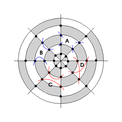
Figure 3.2: Patterns away from the poles

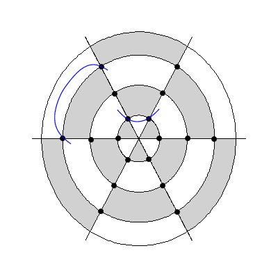
Figure 3.3: Patterns near the poles

The local nodal pattern at the vertices is shown in the domain labelled (A). According to Lemma 3.1, and our assumption on $\mu$, the nodal set $N(H^{\mu,\ell})$ consists of finitely many disjoint simple closed regular curves. According to Properties 3.2.3 (ii), any such nodal curve can only enter a domain ${\cal Q}_{i,j}$ at a vertex, and exit at another one. Taking into account Properties 3.2.3 (iii), this leaves exactly three possibilities for the nodal pattern in a domain ${\cal Q}_{i,j}$, illustrated in the domains labelled (B), (C) and (D). According to the separation Lemma 3.2, both (C) and (D) are impossible. Notice that case (D) could also be discarded by the fact that the nodal curves do not intersect (absence of critical zeros). Finally, the only possible local nodal pattern in the square-like domain ${\cal Q}_{i,j}$ is the one shown in (B): the nodal curves “follow” the meridians.

Remark. In Stern’s thesis this conclusion follows from the claim that the nodal set depends continuously on $\mu$ and that $\mu$ is small enough.

Figure 3.3 is drawn in the case $\ell=3$, but aims at illustrating the possible local nodal patterns in the general case. We look at triangle-like domains ${\cal Q}_{i,j}$ which can be visited by the nodal set, and one of whose vertices is at the north or south pole. This means that $i=0$ or $\ell$, $0\leq j\leq 2\ell-1$ and that $(-1)^{i+j}=-1$, see Properties 3.2.3 (i).

The same arguments as above show that there is only one possible nodal pattern.

3.2.5 A. Stern’s first theorem for the sphere

We can now state the following quantitative version of A. Stern’s first theorem, see Theorem 1.2. Recall the notation $\mu_{c}(\ell)$ in Lemma 3.1.

Proposition 3.3

Assume that $0<\mu<\mu_{c}(\ell)$.

1. When $\ell$ is odd, the nodal set $N(H^{\mu,\ell})$ is a unique regular simple closed curve and hence, the eigenfunction $H^{\mu,\ell}$ has exactly two nodal domains.

2. When $\ell$ is even, the nodal set $N(H^{\mu,\ell})$ is the union of $\ell$ regular disjoint simple closed curves and hence, the eigenfunction $H^{\mu,\ell}$ has exactly $(\ell+1)$ nodal domains.

Proof. According to the remark following Lemma 3.1, under the assumption on $\mu$, the nodal set of $H^{\mu,\ell}$ is a regular $1$-dimensional submanifold. Since the eigenfunction $H^{\mu,\ell}$ does not vanish at the north and south poles, we can work in the exponential map at the north pole. For the proofs below, keep in mind Section 3.2.4.

Proof of Proposition 3.3, Assertion (ii). The integer $\ell$ is assumed to be even. The proof is illustrated by Figure 3.5 which shows parts of the nodal patterns of $Z_{\ell}$ (latitude circles) and $W_{\ell}$ (meridians) viewed in the exponential map centered at the north pole $p_{+}$. The south pole corresponds to the outer circle (the boundary of the maximal domain in which the exponential map is a diffeomorphism).

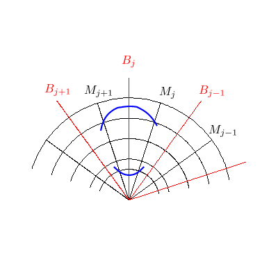
Figure 3.4: $\ell$ even, $j$ odd

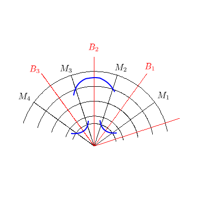
Figure 3.5: $\ell$ odd

Call $B^{\prime}_{j}$ the intersection

$$B^{\prime}_{j}=B_{j}\cap\{\vartheta_{1}(\ell)\leq\vartheta\leq\pi-\vartheta_{1}(\ell)\}.$$

We now use Lemma 3.2.

(a)  When $j$ is even, the function $b^{\,\mu,\ell,j}(\vartheta)$ is positive in $[0,\vartheta_{1}(\ell)]\cup[\pi-\vartheta_{1}(\ell),\pi]$, and hence, by Lemma 3.2, $N(H^{\mu,\ell})\cap B_{j}=\emptyset\,$. When $j$ is odd, the function $b^{\,\mu,\ell,j}(\vartheta)$ has exactly one zero in each of the intervals $(0,\vartheta_{1}(\ell))$ and $(\pi-\vartheta_{1}(\ell),\pi)$. It follows that $N(H^{\mu,\ell})\cap B_{j}$ consists of exactly two points, one in ${\cal Q}_{0,j}$ and one in ${\cal Q}_{\ell,j}$.

(b)  Choose $j=2k+1$, odd (see Figure 3.5). Note that there are exactly $\ell$ such values of $j$ between $0$ and $2\ell-1$. In ${\cal Q}_{0,j}$ the nodal set $N(H^{\mu,\ell})$ can only consist of a curve from the point $q_{1,j}$ to the point $q_{1,j+1}$ (see Subsection 3.1 for the notation, and use Properties 3.2.3), intersecting $B_{j}$ at exactly one point. This curve is part of a connected component (a simple closed curve) $\gamma_{k}\subset N(H^{\mu,\ell})$. We now follow the curve $\gamma_{k}$, starting from $q_{1,j}$ in the direction of $q_{1,j+1}$. According to the preceding point (a), $\gamma_{k}$ can meet neither $B_{j+1}$, nor $B^{\prime}_{j}$. Therefore, according to Paragraph 3.2.4, the curve has to go through the points $q_{1,j+1},q_{2,j+1},\ldots,q_{\ell,j+1}$ passing alternatively inside ${\cal M}_{j+1}$ or ${\cal M}_{j}$. Since $\ell$ is even, at $q_{\ell,j+1}$, the curve enters ${\cal Q}_{\ell,j}$, crosses $B_{j}$ (at a single point), and exits ${\cal Q}_{\ell,j}$ at $q_{\ell,j}$. Since it can cross neither $B_{j-1}$, nor $B^{\prime}_{j}$, the curve $\gamma_{k}$ has to go back to $q_{1,j}$, through the points $q_{\ell-1,j},\ldots,q_{2,j}$, alternatively inside ${\cal M}_{j}$ or ${\cal M}_{j-1}$. This means that the simple closed curve $\gamma_{k}$ goes through all the points in ${\cal N}\cap{\cal M}_{j}$, with $j=2k+1$.

(c)  In this way, we obtain $\ell$ simple closed curves $\gamma_{1},\ldots,\gamma_{\ell}$ which are connected components of $N(H^{\mu,\ell})$, with the curve $\gamma_{k}$ (where $j=2k+1$) contained in the sector bounded by the meridians $B_{j-1}$ and $B_{j+1}$ and containing $B_{j}$. Furthermore, these $\ell$ curves visit all the points $q_{i,j}\in{\cal N}$. It follows from Properties 3.2.3 (iii) that there can be no other components, and hence that

$$N(H^{\mu,\ell})=\cup_{k=1}^{\ell}\gamma_{k}\,.$$

This finishes the proof of Proposition 3.3, Assertion (ii). $\square$

Proof of Proposition 3.3, Assertion (i). The integer $\ell$ is now assumed to be odd. The proof is illustrated by Figure 3.5 which shows parts of the nodal patterns of $Z_{\ell}$ (latitude circles) and $W_{\ell}$ (meridians) viewed in the exponential map centered at the north pole $p_{+}\,$. The south pole corresponds to the outer circle (the boundary of the domain in which the exponential map is a diffeomorphism).

As in the previous proof, call $B^{\prime}_{j}$ the intersection

$$B^{\prime}_{j}=B_{j}\cap\{\vartheta_{1}(\ell)\leq\vartheta\leq\pi-\vartheta_{1}(\ell)\}.$$

(a)  When $j$ is even, the function $b^{\,\mu,\ell,j}(\vartheta)$ is positive in $[0,\vartheta_{1}(\ell)]$, and admits exactly one zero in the interval $(\pi-\vartheta_{1}(\ell),\pi)$. Hence $N(H^{\mu,\ell})\cap B_{j}$ contains exactly one point located in ${\cal Q}_{\ell,j}$. When $j$ is odd, the function $b^{\,\mu,\ell,j}(\vartheta)$ has exactly one zero in the interval $\left(0,\vartheta_{1}(\ell)\right)$ and is negative in $[\pi-\vartheta_{1}(\ell),\pi]$. By Lemma 3.2, it follows that $N(H^{\mu,\ell})\cap B_{j}$ consists of exactly one point located in ${\cal Q}_{0,j}$.

(b)  Choose $j=1$. In ${\cal Q}_{0,1}$ the nodal set $N(H^{\mu,\ell})$ can only consist of a curve going from the point $q_{1,1}$ to the point $q_{1,2}$ (see Subsection 3.1 for the notation and use Properties 3.2.3), intersecting $B_{1}$ at exactly one point. This curve is part of a connected component (a simple closed curve) $\gamma\subset N(H^{\mu,\ell})$. We now follow the curve $\gamma$, starting from $q_{1,1}$ in the direction of $q_{1,2}$. According to the preceding point (a), $\gamma$ can meet neither $B^{\prime}_{2}$, nor $B_{1}$, so that it has to go through the points $q_{1,2},q_{2,2},\ldots,q_{\ell,2}$ passing alternatively inside ${\cal M}_{2}$ or ${\cal M}_{1}$. Because $\ell$ is odd, at $q_{\ell,2}$, the curve exits ${\cal Q}_{\ell-1,1}$, enters ${\cal Q}_{\ell,2}$, crosses $B_{2}$ (at a single point), and exits ${\cal Q}_{\ell,2}$ at $q_{\ell,3}$ into ${\cal M}_{3}$. Since it can cross neither $B^{\prime}_{3}$, nor $B^{\prime}_{2}$, the curve $\gamma$ has to go to $q_{1,3}$, through the points $q_{\ell-1,3},\ldots q_{2,3}$, alternatively inside ${\cal M}_{2}$ or ${\cal M}_{3}$. The curve $\gamma$ therefore goes from $q_{1,1}$ to $q_{1,3}$ where we can start again with the same argument as before. Iterating $\ell$ times the argument, the curve $\gamma$ gets back to its initial point $q_{1,1}$.

(c)  In this way, we obtain a simple closed curve $\gamma$ in $N(H^{\mu,\ell})$, which crosses all the meridians $B_{j}$ once, and which visits all the points $q_{i,j}\in{\cal N}$. It follows from Properties 3.2.3 (iii) that there can be no other component, and hence that

$$N(H^{\mu,\ell})=\gamma\,.$$

This finishes the proof of Proposition 3.3, Assertion (i). $\square$

It is easy to follow the above proofs on Figure 3.6 which shows the nodal set of $H^{\mu,\ell}$, in the exponential map at $p_{+}$, for $\mu>0$ small enough and for $\ell=3$ (left) and $\ell=4$ (right).

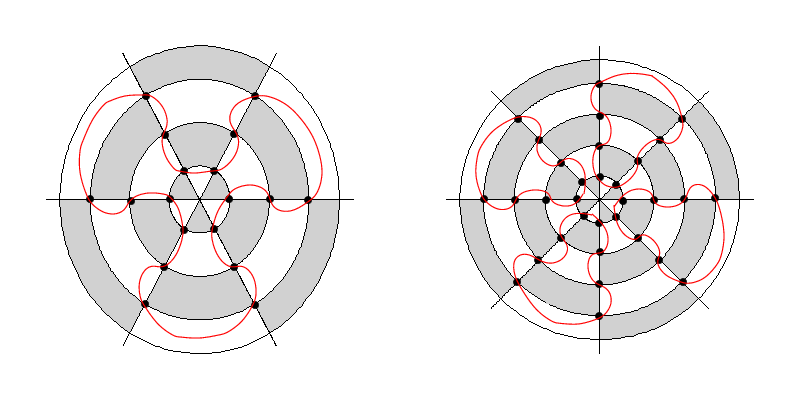
Figure 3.6: Cases $\ell=3$ and $\ell=4$

4 Stern’s second theorem: even case

The purpose of this section is to prove Theorem 1.3. As a matter of fact, we shall give a more quantitative result, Proposition 4.3, which implies the theorem. As in Section 3, we follow the ideas of A. Stern sketched in the introduction.

Fix an integer

$$\ell=2r\geq 2\,,$$

as well as an angle $\alpha$ defined by

$$\alpha=\frac{\epsilon\pi}{2r}\,,\mbox{ with }0<\epsilon<\frac{1}{2}\,.$$ (4.1)

4.1 Notation

As in the first example, we consider the spherical harmonic of degree $\ell=2r$

$$W(x,y,z)=\Im(x+iy)^{2r}\,,$$ (4.2)

whose expression in spherical coordinates $(\vartheta,\varphi)\in\,(0,\pi)\times{\mathbb{R}}_{2\pi}$ is given by

$$w(\vartheta,\varphi)=\sin^{2r}(\vartheta)\,\sin(2r\varphi)\,.$$ (4.3)

The perturbation of $W$ is chosen to be the spherical harmonic $V_{\alpha}$, of degree $2r$, whose expression in spherical coordinates is given by

$$v_{\alpha}(\vartheta,\varphi)=P^{1}_{2r}(\cos\vartheta)\,\sin(\varphi-\alpha)\,.$$ (4.4)

According to Properties 2.2 (i), we have $P^{1}_{2r}(t)=-(1-t^{2})^{1/2}\,\frac{d}{dt}P_{2r}(t)$, so that

$$v_{\alpha}(\vartheta,\varphi)=-\sin\vartheta\,P^{\prime}_{2r}(\cos\vartheta)\,\sin(\varphi-\alpha)\,.$$ (4.5)

According to (2.1), the corresponding harmonic homogeneous polynomial of degree $2r$ in ${\mathbb{R}}^{3}$ is given by the formula

$$V_{\alpha}(x,y,z)=\left(\sin\alpha\,x-\cos\alpha\,y\right)\sum_{j=0}^{r-1}a_{j}z^{2r-2j-1}(x^{2}+y^{2}+z^{2})^{j}\,,$$ (4.6)

where the $a_{j}$’s are the coefficients of the polynomial $P^{\prime}_{2r}$,

$$P^{\prime}_{2r}(t)=\sum_{j=0}^{r-1}a_{j}t^{2r-2j-1}\,.$$

The nodal set of the spherical harmonic $W$ consists of the $2\ell=4r$ meridians $M_{j},0\leq j\leq 4r-1\,$, defined as in Subsection 3.1,

$$N(W)=\bigcup_{j=0}^{4r-1}M_{j}\,,$$

with the corresponding open sectors ${\cal M}_{j}$ on the sphere.

These meridians meet at the north and south poles which are the only critical zeros of $W$, $W(p_{\pm})=0$, and $d_{p_{\pm}}W=0\,$ (the differential of the function $W$ at the poles).

The nodal set of the spherical harmonic $V_{\alpha}$ consists of $(2r-1)$ latitude circles $L^{\prime}_{i}$ ($1\leq i\leq 2r-1$), and two meridians $M^{\prime}_{0}$ and $M^{\prime}_{1}$,

$$N(V_{\alpha})=\bigcup_{j=0}^{2r-1}L^{\prime}_{i}\,\bigcup M^{\prime}_{0}\bigcup M^{\prime}_{1}\,.$$ (4.7)

The latitude circles,

$$L^{\prime}_{i}=\{(\vartheta,\varphi)~{}|~{}\vartheta=\vartheta^{\prime}_{i}(2r)\}\,,~{}1\leq i\leq 2r-1\,,$$ (4.8)

are associated with the $(2r-1)$ zeros, $~{}0<\vartheta^{\prime}_{1}(2r)<\cdots<\vartheta^{\prime}_{2r-1}(2r)<\pi~{}$, of the function $P^{\prime}_{2r}(\cos\vartheta)$, see Properties 2.2 (iii), and we let $\vartheta^{\prime}_{0}(2r)=0$ and $\vartheta^{\prime}_{2r}(2r)=\pi$. They determine sectors

$${\cal L}^{\prime}_{i}=\{(\vartheta,\varphi)~{}|~{}\vartheta^{\prime}_{i}(2r)<\vartheta<\vartheta^{\prime}_{i+1}(2r)\}\,,0\leq i\leq 2r-1\,.$$ (4.9)

The meridians $M^{\prime}_{k}$ are given by

$$M^{\prime}_{0}=\{(\vartheta,\varphi)~{}|~{}\varphi=\alpha\}\text{~{}and~{}}M^{\prime}_{1}=\{(\vartheta,\varphi)~{}|~{}\varphi=\alpha+\pi\}\,.$$ (4.10)

They determine sectors

$${\cal M}^{\prime}_{0}=\{(\vartheta,\varphi)~{}|~{}\alpha<\varphi<\alpha+\pi\}\text{~{}and~{}}{\cal M}^{\prime}_{1}=\{(\vartheta,\varphi)~{}|~{}\alpha+\pi<\varphi<2\pi+\alpha\}\,.$$ (4.11)

Figure 4.2 shows the nodal sets $N(W)$ and $N(V_{\alpha})$, in the case $\ell=2r=4\,$. They are viewed in the exponential map $\exp_{p_{+}}$  i.e., in the disk $D(0,\pi)$, whose boundary corresponds to the cut-locus of $p_{+}$ i.e., $p_{-}$ .

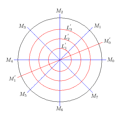
Figure 4.1: $N(W)$ and $N(V_{\alpha})$, $\ell=4$

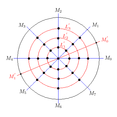
Figure 4.2: ${\cal N}$, $\ell=4$

As in the first example, the set ${\cal N}=N(W)\cap N(V_{\alpha})$ of common zeros to the spherical harmonics $W$ and $V_{\alpha}$, plays a special role. We have

$${\cal N}=\{p_{+},p_{-}\}\bigcup\{q_{i,j}~{}|~{}1\leq i\leq 2r-1,~{}0\leq j\leq 4r-1\}\,,$$ (4.12)

where $q_{i,j}$ is the intersection point of the latitude circle $L^{\prime}_{i}$ with the meridian $M_{j}$.
Figure 4.2 shows the set ${\cal N}$ in the exponential map. The points in ${\cal N}$ appear as the big dots: the intersection points of the latitude circles $L^{\prime}_{i}$, with the meridians $M_{j}$, and the poles. Note that the south pole is represented by two small dots, one on the meridian $M^{\prime}_{0}$, one on the meridian $M^{\prime}_{1}$. Note that there are no other dots on these meridians, see Properties 4.2.4 (iii).

We also introduce the connected components of the set $\{W\,V_{\alpha}\neq 0\}$,

$${\cal Q}_{i,j,k}={\cal L}^{\prime}_{i}\cap{\cal M}_{j}\cap{\cal M}^{\prime}_{k}\,,~{}0\leq i\leq 2r-1,~{}0\leq j\leq 4r-1,~{}k=0,1\,.$$ (4.13)

Note that

$$\mathrm{sgn}(W\,V_{\alpha})=(-1)^{i+j+k+1}\text{~{}on~{}}{\cal Q}_{i,j,k}\,.$$ (4.14)

4.2 The family $H^{\mu}$

4.2.1 Definition

Following the ideas of Stern St , we consider the one-parameter family of spherical harmonics of degree $\ell=2r$,

$$H^{\mu}(x,y,z)=W(x,y,z)-\mu V_{\alpha}(x,y,z)\,,$$ (4.15)

whose expression in spherical coordinates is given by

$$\begin{split}h^{\mu}(\vartheta,\varphi)&=w(\vartheta,\varphi)-\mu\,v_{\alpha}(\vartheta,\varphi)\,,\\ &=\sin^{2r}(\vartheta)\,\sin(2r\varphi)+\mu\,\sin\vartheta\,P^{\prime}_{2r}(\cos\vartheta)\,\sin(\varphi-\alpha)\,.\end{split}$$ (4.16)

Note that

$$h^{-\mu}(\vartheta,\varphi)=h^{\mu}(\vartheta,\varphi+\pi)\,.$$ (4.17)

It follows that it suffices to consider the case $\mu>0$. We shall therefore assume that $\mu>0$ for the remainder of Section 4.

4.2.2 Critical zeros

We now investigate the critical zeros of $H^{\mu}$. The spherical harmonic $W$ vanishes at order at least $3$ at the poles, while the nodal set of $V_{\alpha}$ is a piece of great circle at each pole. It follows that the north and south poles are not critical points of $N(H^{\mu})$, see also Properties 4.2.4 (i). We can therefore look for critical zeros in the spherical coordinates i.e., look for critical zeros of $h^{\mu}$ in $(0,\pi)\times{\mathbb{R}}_{2\pi}$.

The point $(\vartheta,\varphi)\in\,(0,\pi)\times{\mathbb{R}}_{2\pi}$ is a critical zero of $h^{\mu}$ if and only if,

$$\begin{split}&h^{\mu}(\vartheta,\varphi)=0\,,\\ &\partial_{\vartheta}h^{\mu}(\vartheta,\varphi)=0\,,\\ &\partial_{\varphi}h^{\mu}(\vartheta,\varphi)=0\,.\\ \end{split}$$ (4.18)

Using the second order differential equation (2.4) satisfied by the Legendre polynomial $P_{2r}$, we find that

$$\begin{split}\partial_{\vartheta}h^{\mu}(\vartheta,\varphi)=&~{}2r\,\cos\vartheta\,\sin^{2r-1}(\vartheta)\,\sin(2r\varphi)\\ &~{}+\mu\sin(\varphi-\alpha)\big{[}2r(2r+1)P_{2r}(\cos\vartheta)-\cos\vartheta\,P^{\prime}_{2r}(\cos\vartheta)\big{]}\,.\end{split}$$

It follows that the point $(\vartheta,\varphi)\in\,(0,\pi)\times{\mathbb{R}}_{2\pi}$ is a critical zero of $h^{\mu}$ if and only if,

$$\begin{split}&\sin^{2r-1}(\vartheta)\,\sin(2r\varphi)+\mu\,P^{\prime}_{2r}(\cos\vartheta)\,\sin(\varphi-\alpha)=0\,,\\[4.0pt] &2r\,\cos\vartheta\,\sin^{2r-1}(\vartheta)\,\sin(2r\varphi)\\ &~{}~{}+\mu\sin(\varphi-\alpha)\big{[}2r(2r+1)P_{2r}(\cos\vartheta)-\cos\vartheta P^{\prime}_{2r}(\cos\vartheta)\big{]}=0\,,\\[4.0pt] &2r\,\sin^{2r-1}(\vartheta)\,\cos(2r\varphi)+\mu\,P^{\prime}_{2r}(\cos\vartheta)\,\cos(\varphi-\alpha)=0\,.\\ \end{split}$$ (4.19)

The pair of the first and third equations in (4.19) is equivalent to the pair of the first and third equations in (4.20) below. Plugging the first equation in (4.19) into the second one, and using the fact that $\mu>0$, we get the second equation in (4.20). It follows that the point $(\vartheta,\varphi)\in\,(0,\pi)\times{\mathbb{R}}_{2\pi}$ is a critical zero of $h^{\mu}$ if and only if,

$$\begin{split}&\mu\,P^{\prime}_{2r}(\cos\vartheta)+\sin^{2r-1}(\vartheta)\,\big{[}2r\cos(2r\varphi)\,\cos(\varphi-\alpha)+\sin(2r\varphi)\,\sin(\varphi-\alpha)\big{]}=0\,,\\ &\sin(\varphi-\alpha)\,\big{[}2rP_{2r}(\cos\vartheta)-\cos\vartheta P^{\prime}_{2r}(\cos\vartheta)\big{]}=0\,,\\ &2r\cos(2r\varphi)\,\sin(\varphi-\alpha)-\sin(2r\varphi)\,\cos(\varphi-\alpha)=0\,.\end{split}$$ (4.20)

Assume that $\mu>0$. Then, the product $\sin(2r\varphi)\,\sin(\varphi-\alpha)$ does not vanish at the critical zeros of $H^{\mu}$.

This property follows from the third equation in (4.20).

Finally, it follows that the point $(\vartheta,\varphi)\in\,(0,\pi)\times{\mathbb{R}}_{2\pi}$ is a critical zero of $h^{\mu}$ if and only if,

$$\begin{split}\mu\,P^{\prime}_{2r}(\cos\vartheta)+\sin^{2r-1}(\vartheta)\,\big{[}2r\cos(2r\varphi)\,\cos(\varphi-\alpha)+\sin(2r\varphi)\,\sin(\varphi-\alpha)\big{]}&=0\,,\\ 2rP_{2r}(\cos\vartheta)-\cos\vartheta P^{\prime}_{2r}(\cos\vartheta)&=0\,,\\ 2r\cos(2r\varphi)\,\sin(\varphi-\alpha)-\sin(2r\varphi)\,\cos(\varphi-\alpha)&=0\,.\\ \end{split}$$ (4.21)

We first analyze the second equation in (4.21). Define $Q(t):=2rP_{2r}(t)-tP^{\prime}_{2r}(t)\,$. This is an even polynomial of degree less than or equal to $(2r-2)$. For parity reasons the roots of the polynomials $Q,P_{2r}$ and $P^{\prime}_{2r}$ are symmetric with respect to $0\,$, and it suffices to look at $t\geq 0\,$. According to Properties 2.2 (iii), the non-negative roots $t_{i}$ of $P_{2r}\,$, and $t^{\prime}_{i}$ of $P^{\prime}_{2r}$ satisfy

$$0=t^{\prime}_{r}<t_{r}<t^{\prime}_{r-1}<t_{r-1}<\cdots<t_{2}<t^{\prime}_{1}<t_{1}<1\,.$$

The following equalities are easy to check,

$$\mathrm{sgn}({P_{2r}(t^{\prime}_{i})})=(-1)^{i}\text{~{}and~{}}\mathrm{sgn}({P^{\prime}_{2r}(t_{i})})=(-1)^{i-1}\,,$$

$$\mathrm{sgn}({Q(t_{i})})=(-1)^{i}\text{~{}and~{}}\mathrm{sgn}({Q(t^{\prime}_{i-1})})=(-1)^{i-1}\,.$$

It follows that $Q$ vanishes at least once in each interval $(t_{i+1},t^{\prime}_{i})$ for $1\leq i\leq r-1\,$. Since $Q$ has at most $(r-1)$ non-negative zeros, we can conclude that $Q$ has exactly $(r-1)$ zeros in $(0,1)$, and more precisely one zero, which we denote by $\cos\omega_{i}$, in each interval $(t_{i+1},t^{\prime}_{i})$, so that $\omega_{i}\in\,(\vartheta^{\prime}_{i}(2r),\vartheta_{i+1}(2r))$, and

$$0<\vartheta_{1}(2r)<\vartheta^{\prime}_{1}(2r)<\omega_{1}<\vartheta_{2}(2r)<\cdots<\vartheta^{\prime}_{r-1}(2r)<\omega_{r-1}<\vartheta_{r}(2r)<\vartheta^{\prime}_{r}(2r)=\frac{\pi}{2}\,.$$

Note that the inequalities are strict i.e., that $P_{2r}(\cos\omega_{i})\neq 0$ and $P^{\prime}_{2r}(\cos\omega_{i})\neq 0\,$, and that the zeros $\omega_{i}$ depend on $\ell=2r\,$.

We now analyze the third equation in (4.21). Define the function,

$$f(\varphi)=2r\,\cos(2r\varphi)\,\sin(\varphi-\alpha)-\sin(2r\varphi)\,\cos(\varphi-\alpha)\,.$$ (4.22)

The function $f$ satisfies $f(\pi+\varphi)+f(\varphi)=0\,$, and $f^{\prime}(\varphi)=-(4r^{2}-1)\sin(2r\varphi)\,\sin(\varphi-\alpha)\,$. An easy analysis in $[0,\pi]$ (using the choice of $\alpha$) shows that $f$ does not vanish in $[0,\frac{\pi}{2r}]$, and has exactly one zero in each interval $[j\frac{\pi}{2r},(j+1)\frac{\pi}{2r}]$ for $1\leq j\leq 2r-1\,$. It follows that $f$ has exactly $(4r-2)$ zeros in $[0,2\pi]$, $0<\varphi_{1}<\varphi_{2}<\cdots<\varphi_{4r-2}<2\pi$, and that $\varphi_{j}\in\left(j\frac{\pi}{2r},(j+1)\frac{\pi}{2r}\right)$.

The only possible critical zeros of $H^{\mu}$ are given in spherical coordinates by the points $(\omega_{i},\varphi_{j})$ and $(\pi-\omega_{i},\varphi_{j})\,$, for $1\leq i\leq r-1$ and $1\leq j\leq 4r-2\,$. These points can only occur as critical zeros for finitely many values of $\mu$ given by the first equation in (4.21). Since we work with $\mu>0$, these critical values of $\mu$ are given (see also the first line in (4.19)) by

$$\mu_{i,j}(\alpha)=\Big{|}\frac{\sin^{2r-1}(\omega_{i})\,\sin(2r\varphi_{j})}{P^{\prime}_{2r}(\cos\omega_{i})\,\sin(\varphi_{j}-\alpha)}\Big{|}\,,$$ (4.23)

for $1\leq i\leq r-1,~{}~{}1\leq j\leq 2r-1\,$, and can be numerically computed.
We summarize the preceding analysis in the following lemma.

Lemma 4.1

For $\mu>0\,$, the spherical harmonic $H^{\mu}$ has no critical zero except for finitely many values of $\mu$ which are given by (4.23). For each value $\mu_{i,j}(\alpha)\,$, the spherical harmonic $H^{\mu}$ has finitely many critical zeros. Define the number $\mu_{c}(\alpha,2r)$ to be

$$\mu_{c}(\alpha,2r)=\inf\mu_{i,j}(\alpha)\,,$$ (4.24)

where the infimum is taken over $1\leq i\leq r-1\,$, and $1\leq j\leq 2r-1\,$. Then, for $0<\mu<\mu_{c}(\alpha,2r)\,$, the function $H^{\mu}$ has no critical zero, so that its nodal set $N(H^{\mu})$ consists of finitely many disjoint simple closed curves.

Remark. One can bound $\mu_{c}(\alpha,2r)$ from below using the inequalities satisfied by the $\omega_{i}$, and Properties 2.2 (vii).

4.2.3 A separation lemma for $N(H^{\mu})$

For $1\leq j\leq 4r-2\,$, call $C_{j}$ the meridian,

$$C_{j}=\{(\vartheta,\varphi)~{}|~{}\varphi=\varphi_{j}\}\,,$$ (4.25)

where $\varphi_{j}$ are the zeros of the function $f$ defined in (4.22).

We now look at the restriction of the spherical harmonic $H^{\mu}$ to the meridian $C_{j}$. Recall from Properties 2.2 (iii), that $\cos\vartheta^{\prime}_{1}(2r)$ is the largest zero of the function $P^{\prime}_{2r}(\cos\vartheta)$ in $[0,\pi]$.

Lemma 4.2

Define the functions,

$$\begin{split}b^{\,\mu,j}(\vartheta)&=h^{\mu}(\vartheta,\varphi_{j})\\ &=\sin(2r\varphi_{j})\,\sin^{2r}(\vartheta)+\mu\,\sin\vartheta\,P^{\prime}_{2r}(\cos\vartheta)\,\sin(\varphi_{j}-\alpha)\,.\end{split}$$ (4.26)

Assume that $2r+1\leq j\leq 4r-1$.

1. For $0<\mu<\mu_{c}(\alpha,2r)$, the functions $b^{\,\mu,j}(\vartheta)$ do not vanish in the interval $[\vartheta^{\prime}_{1}(2r),\pi-\vartheta^{\prime}_{1}(2r)]$.

2. When $j$ is odd, the function $b^{\,\mu,j}(\vartheta)$ vanishes exactly once in the interval $\left(0,\vartheta^{\prime}_{1}(2r)\right)$, and does not vanish in the interval $[\pi-\vartheta^{\prime}_{1}(2r),\pi]$.

3. When $j$ is even, the function $b^{\,\mu,j}(\vartheta)$ vanishes exactly once in the interval $(\pi-\vartheta^{\prime}_{1}(2r),\pi)$, and does not vanish in the interval $[0,\vartheta^{\prime}_{1}(2r)]$.

The above assertions determine the possible intersections of the nodal set $N(H^{\mu})$ with the meridian $C_{j}$.

Proof. Notice that the assumptions on $j$ and $\alpha$ imply that $\sin(\varphi_{j}-\alpha)<0$, and that $(-1)^{j}\sin(2r\varphi_{j})>0$. The function $b^{\,\mu,j}$ vanishes at the points such that

$$\frac{\sin\vartheta\,P^{\prime}_{2r}(\cos\vartheta)}{\sin^{2r}(\vartheta)}=-\frac{\sin(2r\varphi_{j})}{\mu\,\sin(\varphi_{j}-\alpha)}\,.$$

Call $\beta_{2}(\vartheta)$ the function in the left-hand side. Using the differential equation satisfied by $P_{2r}$, one finds that

$$\beta^{\prime}_{2}(\vartheta)=(2r+1)\,\frac{2r\,P_{2r}(\cos\vartheta)-\cos\vartheta\,P^{\prime}_{2r}(\cos\vartheta)}{\sin^{2r}(\vartheta)}\,.$$

The local extrema of $\beta_{2}$ in the interval $[\vartheta^{\prime}_{1}(2r),\pi-\vartheta^{\prime}_{1}(2r)]$ are achieved at the zeros $\omega_{i}\in\left(\vartheta^{\prime}_{i}(2r),\vartheta_{i+1}(2r)\right)$ of the second equation in (4.21), for $1\leq i\leq 2r-2$. We have at these points,

$$h^{\,\mu}(\omega_{i},\varphi_{j})=\sin(2r\varphi_{j})\,\sin^{2r}(\omega_{i})\,\Big{[}1+\mu\,\frac{P^{\prime}_{2r}(\cos\omega_{i})\,\sin(\varphi_{j}-\alpha)}{\sin(2r\varphi_{j})\,\sin^{2r-1}(\omega_{i})}\Big{]}.$$

The first assertion follows from (4.23).

We now determine what happens in the intervals $\left(0,\vartheta^{\prime}_{1}(2r)\right)$ and $(\pi-\vartheta^{\prime}_{1}(2r),\pi)$.

Write $b^{\,\mu,j}(\vartheta)=(-1)^{j}\,\sin\vartheta\,f_{j}(\vartheta)$. The derivative $f^{\prime}_{j}(\vartheta)$ is given by

$$f^{\prime}_{j}(\vartheta)=(2r-1)\,(-1)^{j}\,\sin(2r\varphi_{j})\,\cos\vartheta\,\sin^{2r-2}(\vartheta)-(-1)^{j}\,\mu\,\sin\vartheta\,P^{{}^{\prime\prime}}_{2r}(\cos\vartheta)\sin(\varphi_{j}-\alpha)\,.$$

Recall that $P_{2r}$ and $P^{{}^{\prime\prime}}_{2r}$ are even functions and that $P^{\prime}_{2r}$ is odd. The largest zeros of theses functions in $[-1,1]$ satisfy, with an obvious notation,

$$t_{2}<t^{{}^{\prime\prime}}_{1}<t^{\prime}_{1}<t_{1}<1\,.$$

Looking at the signs of these functions in the various intervals between $t_{2}$ and $1$, and using the parity to determine what happens near $-1\,$, we can make the following observations.

$\bullet$ Case $j$ even. For $\vartheta\in\left(0,\vartheta^{\prime}_{1}(2r)\right)$, $f_{j}(\vartheta)>0$. On the other-hand, $f_{j}\left(\pi-\vartheta^{\prime}_{1}(2r)\right)>0$ and $f_{j}(\pi)<0\,$, while $f^{\prime}_{j}(\vartheta)<0$ in $\left(\pi-\vartheta^{\prime}_{1}(2r),\pi\right)\,$.

$\bullet$ Case $j$ odd. For $\vartheta\in\left(\pi-\vartheta^{\prime}_{1}(2r),\pi\right)$, $f_{j}(\vartheta)>0\,$. On the other-hand, $f_{j}(0)<0$ and $f_{j}\left(\vartheta^{\prime}_{1}(2r)\right)>0\,$, while $f^{\prime}_{j}(\vartheta)>$ in $\left(0,\vartheta^{\prime}_{1}(2r)\right)\,$.

The second and third assertion follows. $\square$

4.2.4 General properties of $N(H^{\mu})$

For $\mu>0$, the nodal sets $N(H^{\mu})$ share the following properties.

1. The north and south poles are zeros of order $1$ of $H^{\mu}$, $H^{\mu}(p_{\pm})=0$, and $d_{p_{\pm}}H^{\mu}\neq 0$. In particular, near each pole, the nodal set $N(H^{\mu})$ consists of a single arc, tangent to the great circle $M^{\prime}_{0}\cup M^{\prime}_{1}$.

2. The nodal set $N(H^{\mu})$ satisfies,

   $${\cal N}\subset N(H^{\mu})\subset{\cal N}\,\bigcup\,\{W\,V_{\alpha}>0\}\,.$$ (4.27)

3. Since $\alpha=\frac{\epsilon\pi}{2r}$, with $0<\epsilon<\frac{1}{2}$, the nodal set $N(H^{\mu})$ meets the great circle $M^{\prime}_{0}\cup M^{\prime}_{1}$ at the poles tangentially, and nowhere else.

4. The connected components of $N(H^{\mu})$ are contained in either the closed hemisphere $\overline{{\cal M}^{\prime}_{0}}$ or in $\overline{{\cal M}^{\prime}_{1}}$.

5. The points in ${\cal N}$ (common zeros to the spherical harmonics $W$ and $V_{\alpha}$) are not critical zeros of $H^{\mu}$. At the points $q_{i,j}\in{\cal N},~{}1\leq i\leq 2r-1,~{}0\leq j\leq 4j-1\,$, the nodal set $N(H^{\mu})$ consists of a single arc which is transversal to the latitude circles $L^{\prime}_{i}$ and to the meridians $M_{j}$.

6. For $0<\mu<\mu_{c}(\alpha,2r)$ (defined in (4.24)), no closed component of the nodal set $N(H^{\mu})$ can be entirely contained in some domain ${\cal Q}_{i,j,k}$.

Proof. Assertion (i) follows from the fact that near the poles, $N(V_{\alpha})$ is a piece of great circle, while $W$ vanishes at order at least $3$. Assertion (ii) is clear (this is the checkerboard property introduced by A. Stern as we recalled in the introduction). Assertion (iii) is clear because the great circle $M^{\prime}_{0}\cup M^{\prime}_{1}$ only meets the nodal set $N(W)$ at the poles. Assertion (iv) follows from Assertion (ii), the choice of $\alpha$ and the parity of $\ell=2r$. We can indeed look at a neighborhood of the north pole (the pattern near the south pole is the image of the pattern at the north pole under the antipodal map). The nodal curve at $p_{+}$ must visit the domains ${\cal Q}_{0,0,1}$ and ${\cal Q}_{0,2r,1}$, both in ${\cal M}^{\prime}_{1}$, and cannot visit the domains ${\cal Q}_{0,0,0}$ and ${\cal Q}_{0,2r,0}$. On the other-hand, as we already pointed out, the nodal set cannot meet the great circle $M^{\prime}_{0}\cup M^{\prime}_{1}$. Assertion (v) follows by checking that the partial derivatives $\partial_{\vartheta}h^{\mu}$ and $\partial_{\varphi}h^{\mu}$ do not vanish at the points $\left(\vartheta^{\prime}_{i}(2r),\frac{j\pi}{2r}\right)$. Assertion (vi) follows by using the same energy argument as in Properties 3.2.3. $\square$

Figure 4.4 illustrates the proof of Properties 4.2.4. The checkerboard appears in white/grey (allowed / forbidden domains).

4.2.5 Local nodal patterns for $H^{\mu}$

The arguments to determine the local nodal patterns for $H^{\mu}$ are the same as in Paragraph 3.2.4, with an extra case. Namely, at each pole, the nodal set $N(H^{\mu})$ is a single arc tangent to the great circle $M^{\prime}_{0}\cup M^{\prime}_{1}$, going through two triangle-like domains, one of whose vertices is the pole. One of the two remaining vertices does not belong to ${\cal N}$, the other does belong to ${\cal N}$ so that the local nodal pattern is well determined. See Figures 3.3, 3.3 and 4.4.

4.2.6 A. Stern’s second theorem

We can now state the following improved version of Stern’s second theorem, Theorem 1.3. Recall the definition of $\mu_{c}(\alpha,2r)$ given in (4.24).

Proposition 4.3

For $\alpha$ satisfying (4.1) and $0<\mu<\mu_{c}(\alpha,2r)\,$,

1. the spherical harmonic $H^{\mu}$, of degree $2r$, introduced in (4.15), has no critical zero,

2. the nodal set $N(H^{\mu})$ of $H^{\mu}$ has exactly two connected components i.e., consists of exactly two simple closed curves which do not intersect.

In particular, for $0<\mu<\mu_{c}(\alpha,2r)$, the spherical harmonic $H^{\mu}$ has exactly three nodal domains.

Proof of Proposition 4.3

Note that $H^{\mu}$ is even, so that it is invariant under the antipodal map, and so is its nodal set $N(H^{\mu})$. We have already seen, Properties 4.2.4, that a connected component of $N(H^{\mu})$ is contained in either $\overline{{\cal M}^{\prime}_{0}}$ or $\overline{{\cal M}^{\prime}_{1}}$. Furthermore, there is one connected component, call it $\gamma$, which is contained in $\overline{{\cal M}^{\prime}_{1}}$, and which is tangent to the great circle $M^{\prime}_{0}\cup M^{\prime}_{1}$ at the north pole $p_{+}$. Similarly, there is another connected component which is contained in $\overline{{\cal M}^{\prime}_{0}}$, and which is tangent to $M^{\prime}_{0}\cup M^{\prime}_{1}$ at the south pole $p_{-}$. The second can be deduced from $\gamma$ by applying the antipodal map.

It follows that it suffices to look at the part of the nodal set $N(H^{\mu})$ which is contained in $\overline{{\cal M}^{\prime}_{1}}$. For this reason, we only have to consider the meridians $C_{j}$ for $2r+1\leq j\leq 4r-1$. The connected component $\gamma$ is a simple closed curve. Start from the north pole, tangentially to $M^{\prime}_{0}$, inside the domain ${\cal Q}_{0,0,1}\,$. The only possibility for $\gamma$ is to exit ${\cal Q}_{0,0,1}$ through the point $q_{1,0,1}$. Using the separation lemma, Lemma 4.1, and the analysis of local nodal patterns, we see that $\gamma$ has to wind around $M_{0}$, inside the white domains, until it reaches the last point $q_{2r-1,0,1}\,$, at which it has to enter the white domain ${\cal Q}_{2r-1,4r-1,1}\,$, cross the meridian $B_{4r-1}$, exit through the point $q_{2r-1,4r-1,1}$ and wind along $M_{4r-1}$ until it reaches the domain ${\cal Q}_{0,4r-2,1}\,$, etc . The situation is similar to the one we encountered in the proof of Proposition 3.3 (i). Indeed, the important point in this proof was that the number $\ell$ of latitude circle $L_{i}$ was odd. In the present case we have $\ell=2r$, but the number of latitude circles $L^{\prime}_{i}$ is $2r-1$, an odd integer. The proof of Section 3 applies mutatis mutandis, and the conclusion is that $\gamma$ goes back to the north pole after going up and down $r$ times, visiting all the points in ${\cal N}\cap{\cal M}^{\prime}_{1}$. Using Properties 4.2.4, it follows that $N(H^{\mu})\cap\overline{{\cal M}^{\prime}_{1}}$ has exactly one connected component $\gamma$. Using the antipodal map, this means that $N(H^{\mu})$ has exactly two connected components. $\square$

Figure 4.4 shows the nodal pattern of $H^{\mu}$ in the exponential map, with one component tangent to the great circle $M^{\prime}_{0}\cup M^{\prime}_{1}$ at the north pole, the other at the south pole.

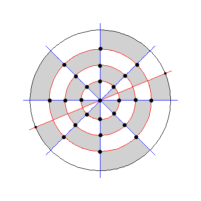
Figure 4.3: Checkerboard: $\ell=4$, $\mu>0$

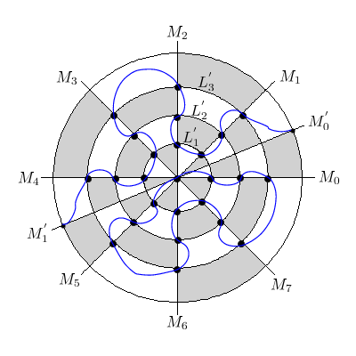
Figure 4.4: $N(H^{\mu})$

5 Courant sharp property and open questions for minimal partitions for the sphere.

Leydold’s thesis Ley (see also a preliminary analysis in LeyD ) is devoted to this question. We reproduce below some synthesis essentially extracted from HHOT1 . Given a spherical harmonic $u$, let $\mu(u)$ denote the number of nodal domains of $u$ (this notation should not induce confusion with the parameter $\mu$ appearing in the preceding sections).

• Courant’s theorem for the sphere says that for any $u_{\ell}\in{\cal H}_{\ell}$,

  $$\mu(u_{\ell})\leq\ell^{2}+1\,,$$

  where the right-hand side is $1+\sum_{k=0}^{\ell-1}\dim{\cal H}_{k}$;

• Pleijel’s asymptotic bound for the number of nodal domains extends to bounded domains in $\mathbb{R}^{n}$, and more generally to compact $n$-manifolds with boundary, with a universal constant $\gamma(n)<1$ replacing the constant $\gamma(2)=4/(j_{0,1})^{2}$ in the right-hand side of (5.1) (Peetre Pe , Bérard-Meyer BeMe ). It is also interesting to note that this constant is independent of the geometry. In particular Pleijel’s theorem is true in the case of the sphere. For any sequence of eigenfunctions $u_{\ell}\in\mathcal{H}_{\ell}$

  $$\lim\sup_{\ell\rightarrow+\infty}\frac{\mu(u_{\ell})}{\ell^{2}+1}\leq\frac{4}{(j_{0,1})^{2}}\,.$$ (5.1)

• Leydold stated the following conjecture on the maximal cardinal of nodal sets of a spherical harmonic.

  Conjecture 5.1

  $$\max_{u\in\mathcal{H}_{\ell}}\mu(u)=\left\{\begin{array}[]{ll}\frac{1}{2}(\ell+1)^{2}&\mbox{ if }\ell\mbox{ is odd, }\\[4.0pt] \frac{1}{2}\ell(\ell+2)&\mbox{ if }\ell\mbox{ is even. }\end{array}\right.$$

  The values in the right hand side are the maximum numbers of nodal domains of the decomposed spherical harmonics in spherical coordinates. This conjecture is proved in Ley for $\ell\leq 6$. Note that the example treated in Appendix A for $\ell=3$ (middle subfigure in Fig. A.3) shows the optimality in this case. In LeyT , Leydold constructs regular spherical harmonics of degree $\ell$ with $O(\frac{\ell^{2}}{4})$ nodal domains, see also (ErJaNa, , Theorem 2.1).

  Conjecture 5.1 implies that the only Courant sharp situations (that is situations in which Courant’s upper bound is attained in some eigenspace) correspond to the first and second eigenvalues. This last statement is true as a consequence of a theorem à la Courant, using the symmetry or antisymmetry of spherical harmonics under the antipodal map, or as a corollary of the following theorem by Karpushkin Ka .

  Theorem 5.2

  $$\max_{u\in\mathcal{H}_{\ell}}\mu(u)\leq\left\{\begin{array}[]{ll}\ell(\ell-2)+5&\mbox{ if }\ell\mbox{ is odd, }\\ \ell(\ell-2)+4&\mbox{ if }\ell\mbox{ is even. }\end{array}\right.$$

  Conjecture 5.1 implies the following inequality which improves Pleijel’s theorem.

  Conjecture 5.3

  For any sequence of eigenfunctions $u_{\ell}\in\mathcal{H}_{\ell}$, we have

  $$\lim\sup_{\ell\rightarrow+\infty}\frac{\mu(u_{\ell})}{\ell^{2}+1}\leq\frac{1}{2}\,.$$ (5.2)

  It is easy to see that (5.2) cannot be improved (look at product eigenfunctions).

• Spectral minimal partitions are for example defined in HHOT . Motivated by a conjecture in harmonic analysis popularized by Bishop Bis (who refers to FrHa ), the authors of HHOT have proved in HHOT1 that up to rotation the minimal $3$-partition is the so-called $Y$-partition ($\{0<\phi<\frac{2\pi}{3}\}$, $\{\frac{2\pi}{3}<\phi<\frac{4\pi}{3}\}$, and $\{\frac{4\pi}{3}<\phi<2\pi\}$). There is a conjecture that the four faces of a spherical tetrahedron determine a minimal $4$-partition on $\mathbb{S}^{2}$. What we get from the previous item and the general theory of HHOT (nodal minimal partitions should correspond to a Courant sharp situation) is that minimal $k$-partitions cannot be nodal for $k>2$.

• With a different point of view, let us mention the contributions of NaSo on random spherical harmonics.

Appendix A Some simulations with Maple

In this appendix, we provide some pictures issued from numerical computations with Maple. The nodal sets are viewed in the exponential map at the north pole. The outer circle, at distance $\pi$, is the cut-locus of $p_{+}$ and corresponds to the south pole.

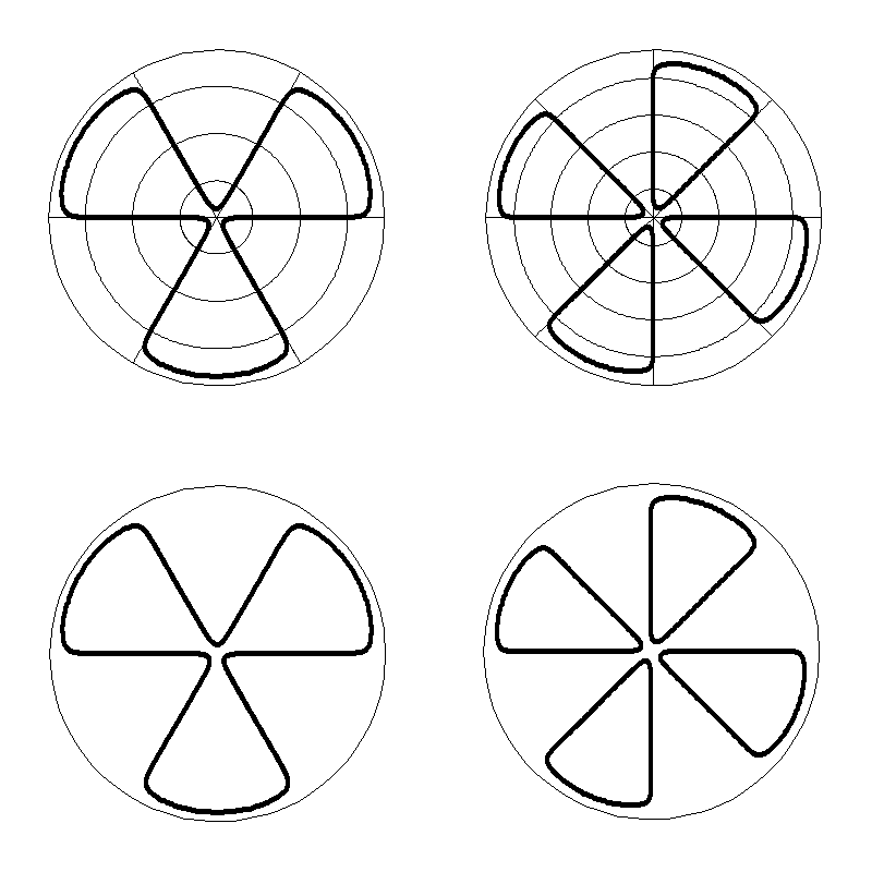
Figure A.1: Example 1: $\ell=3$ and $\ell=4$

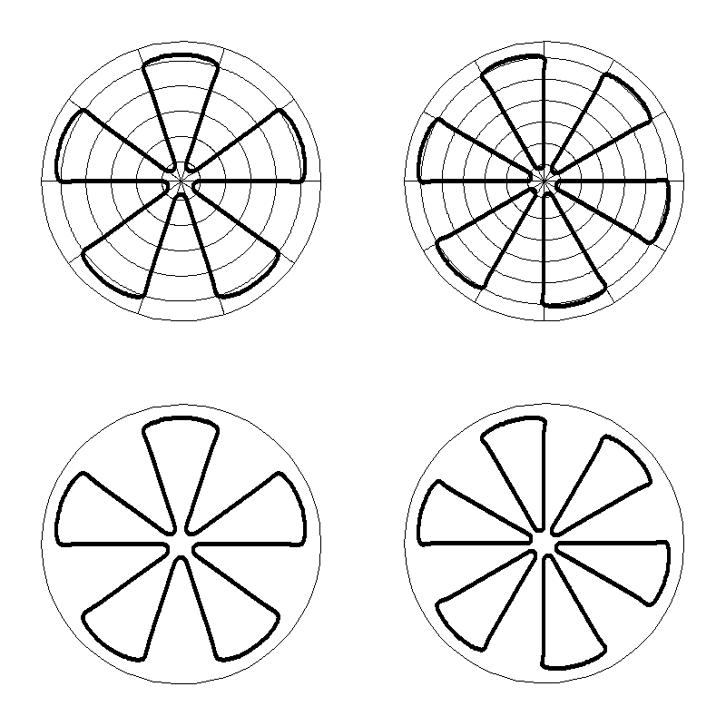
Figure A.2: Example 1: $\ell=5$ and $\ell=6$

Figures A.2 resp. A.2 illustrate Proposition 3.3 in the cases $\ell=3$ (left) and $\ell=4$ (right), resp. $\ell=5$ (left) and $\ell=6$ (right). They display the nodal set of $H^{\mu,\ell}$ (black thick line), with $\mu=5\cdot 10^{-3}$ when $\ell$ is odd, and $\mu=2\cdot 10^{-3}$ when $\ell$ even. The figures in the top line also display the checkerboards associated with $Z_{\ell}$ and $W_{\ell}$.

Figure A.3 illustrates the occurrence of critical zeros in Stern’s Example 1, with $\ell=3$. The corresponding Legendre polynomial is $P_{3}(t)=\frac{1}{2}\,t\,(5t^{2}-3)\,$. The polynomial $P_{2}(t)=\frac{1}{2}\,(3t^{2}-1)$ has two roots $\pm\,\frac{1}{\sqrt{3}}\,$. According to Section 3.2.1, there are twelve possible critical zeros, given in spherical coordinates by the points $\left(\arccos(\pm\frac{1}{\sqrt{3}}),j\frac{\pi}{6}\right)$ with $j\in\{1,3,5,7,9,11\}$, and exactly two critical values of the parameter, $\mu=\pm\,\sqrt{2}\,$. For $\mu>0$, there is exactly one critical value $\mu=\sqrt{2}$, which is associated with six critical zeros. Figure A.3 shows the nodal set $N(H^{\mu,3})$ for $\mu<\sqrt{2}$ (left), for $\mu=\sqrt{2}$ (center) and for $\mu>\sqrt{2}$ (right).

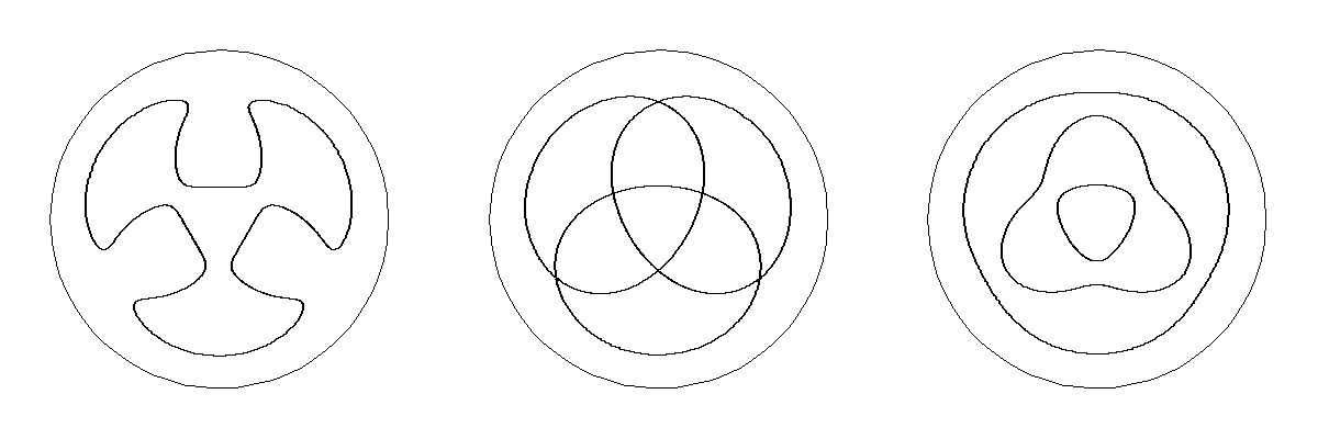
Figure A.3: Appearance and disappearance of critical zeros

Figure A.4 illustrates Proposition 4.3. The figures display the nodal set of the function $H^{\mu}$ (thick lines), with $\mu=10^{-3}$ and $\varepsilon=0.4$. The figures in the top line also display the checkerboards associated with $W,V_{\alpha}$. The great circle $M^{\prime}_{0}\cup M^{\prime}_{1}$ divides the sphere into two closed hemispheres. Each one contains a simple closed nodal curve tangent to the great circle at one of the poles. As usual, the south pole is represented by the outer circle (dotted line), the cut-locus of $0$ in the tangent space at $p_{+}$.

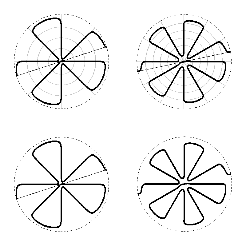
Figure A.4: Example 2: $\ell=4$ and $\ell=6$

Appendix B Translation of citations from Stern’s thesis

We provide below a rough translation of the citations from Stern’s thesis in Section 1

[E1] …one can for example easily show that on the sphere the numbers $2$ or $3$ occur as number of nodal domains for each eigenvalue, and that for the square, if we arrange the eigenvalues in increasing order, the number $2$ always reappears as number of nodal domains.

[K1] We shall then show that for each eigenvalue there exist eigenfunctions on the sphere whose nodal lines divide the sphere into $2$ or $3$ nodal domains only …The number of nodal domains $2$ occurs for the eigenvalues $\lambda_{n}=(2r+1)(2r+2)\,~{}r=1,2,\cdots$;
[K2] similarly, we shall now show that $3$ occurs as number of nodal domains for all eigenvalues $\lambda_{n}=2r(2r+1),~{}r=1,2,\cdots$.

[I1] Superimpose the systems of nodal lines of the two functions, and hatch the domains in which the functions have the same sign, then the nodal lines of the spherical function

$$P^{2r+1}_{2r+1}(\cos\vartheta)\cos(2r+1)\varphi+\mu P_{2r+1}(\cos\vartheta)\,,\quad\mu>0$$

can only pass in the non-hatched domains
[I3]  and hence for values of $\mu$ which are small enough, they stay in a neighborhood of the nodal lines of

$$P^{2r+1}_{2r+1}(\cos\vartheta)\cos(2r+1)\varphi,$$

i.e.  the $2r+1$ meridians, so that the system of nodal lines varies continuously with $\mu$ ….
[I2] Furthermore, the nodal lines must pass through the $2(2r+1)^{2}$ intersection points of the system of nodal lines of the two above spherical functions …

References

- [1] P. Bérard and D. Meyer. Inégalités isopérimétriques et applications. Annales scientifiques de l’École Normale Supérieure, 15:3 (1982), 513-541.
- [2] P. Bérard and B. Helffer. Dirichlet eigenfunctions of the square membrane: Courant’s property, and A. Stern’s and Å. Pleijel’s analyses. arXiv:14026054. To appear in Springer Proceedings in Mathematics & Statistics (2015), MIMS-GGTM conference in memory of M. S. Baouendi. A. Baklouti, A. El Kacimi, S. Kallel, and N. Mir Editors.
- [3] C.J. Bishop. Some questions concerning harmonic measure. Dahlberg, B. (ed.) et al., Partial Differential equations with minimal smoothness and applications. IMA Vol. Math. Appl. 42 (1992), 89-97.
- [4] R. Courant. Ein allgemeiner Satz zur Theorie der Eigenfunktionen selbstadjungierter Differentialausdrücke. Nachr. Ges. Göttingen (1923), 81-84.
- [5] R. Courant and D. Hilbert. Methods of Mathematical Physics. Volume 1. John Wiley & Sons, 1989.
- [6] A. Eremenko, D. Jakobson, and N. Nadirashvili. On nodal sets and nodal domains on . Annales Institut Fourier 57:7 (2007), 2345-2360.
- [7] S. Friedland and W.K. Hayman. Eigenvalue inequalities for the Dirichlet problem on spheres and the growth of subharmonic functions. Comment. Math. Helvetici 51 (1976), 133-161.
- [8] B. Helffer, T. Hoffmann-Ostenhof and S. Terracini. Nodal domains and spectral minimal partitions. Annales Institut Henri Poincaré (Analyse non linéaire) 26 (2009), 101-138.
- [9] B. Helffer, T. Hoffmann-Ostenhof and S. Terracini. On spectral minimal partitions: the case of the sphere. Around the research of Vladimir Maz’ya. III, p. 153-178, Int. Math. Ser. 13, Springer (N.Y.) 2010.
- [10] B. Helffer and M. Persson Sundqvist. Nodal domains in the square–the Neumann case–. arXiv: 1410.6702.
- [11] V.N. Karpushkin. Topology of the zeros of eigenfunctions. Funktional Anal. i Prilozehen 23:3 (1989), 59-60.
- [12] H. Lewy. On the minimum number of domains in which the nodal lines of spherical harmonics divide the sphere. Comm. Partial Differential Equations 2:12 (1977), 1233-1244.
- [13] J. Leydold. Knotenlinien und Knotengebiete von Eigenfunktionen. Diplom Arbeit, Universität Wien (1989), unpublished. Available at http://othes.univie.ac.at/34443/
- [14] J. Leydold. Nodal properties of spherical harmonics. Dissertation Universität Wien (January 1993).
- [15] J. Leydold. On the number of nodal domains of spherical harmonics. Topology 35 (1996), 301-321.
- [16] W. Magnus, F. Oberhettinger, and R.P. Soni. Formulas and Theorems for the Special Functions of Mathematical Physics. Third Edition. Berlin: Springer-Verlag, 1966.
- [17] F. Nazarov and M. Sodin. On the number of nodal domains of random spherical harmonics. Amer. J. Math. 131 (2009), 1337-1357.
- [18] J. Peetre. A generalization of Courant nodal theorem. Math. Scandinavica 5 (1957), 15-20.
- [19] Å. Pleijel. Remarks on Courant’s nodal theorem. Comm. Pure. Appl. Math. 9 (1956), 543-550.
- [20] I. Polterovich. Pleijel’s nodal domain theorem. Proc. Amer. Math. Soc. 137 (2009), 1021-1024.
- [21] A. Stern. Bemerkungen über asymptotisches Verhalten von Eigenwerten und Eigenfunktionen. Inaugural-Dissertation zur Erlangung der Doktorwürde der Hohen Mathematisch-Naturwissenschaftlichen Fakultät der Georg August-Universität zu Göttingen (30 Juli 1924). Druck der Dieterichschen Univertisäts-Buchdruckerei (W. Fr. Kaestner). Göttingen, 1925
- [22] A. Stern. Bemerkungen über asymptotisches Verhalten von Eigenwerten und Eigenfunktionen. Diss. Göttingen (30 Juli 1924). Extracts and annotations by P. Bérard and B. Helffer. Available at http://www-fourier.ujf-grenoble.fr/~pberard/R/stern-1925-thesis-partial-reprod.pdf
- [23] G. Szegö. Orthogonal Polynomials. Fourth edition. Amer. Math. Soc. Colloquium Publications, Vol. XXIII, Amer. Math. Soc. Providence, R.I. (1975).