Optical Properties of (162173) 1999 JU3:
In Preparation for the JAXA Hayabusa 2 Sample Return Mission

Abstract

We investigated the magnitude–phase relation of (162173) 1999 JU3, a target asteroid for the JAXA Hayabusa 2 sample return mission. We initially employed the international Astronomical Union’s $H$–$G$ formalism but found that it fits less well using a single set of parameters. To improve the inadequate fit, we employed two photometric functions, the Shevchenko and Hapke functions. With the Shevchenko function, we found that the magnitude–phase relation exhibits linear behavior in a wide phase angle range ($\alpha$ = 5–75°) and shows weak nonlinear opposition brightening at $\alpha<$ 5°, providing a more reliable absolute magnitude of $H_{\mathrm{V}}$ = 19.25 $\pm$ 0.03. The phase slope (0.039 $\pm$ 0.001 mag deg^-1) and opposition effect amplitude (parameterized by the ratio of intensity at $\alpha$=0.3° to that at $\alpha$=5°, $I(0.3\arcdeg)$/$I(5\arcdeg)$=1.31$\pm$0.05) are consistent with those of typical C-type asteroids. We also attempted to determine the parameters for the Hapke model, which are applicable for constructing the surface reflectance map with the Hayabusa 2 onboard cameras. Although we could not constrain the full set of Hapke parameters, we obtained possible values, $w$=0.041, $g$=-0.38, $B_{0}$=1.43, and $h$=0.050, assuming a surface roughness parameter $\bar{\theta}$=20°. By combining our photometric study with a thermal model of the asteroid (Müller et al. in preparation), we obtained a geometric albedo of $p_{\mathrm{v}}$ = 0.047 $\pm$ 0.003, phase integral $q$ = 0.32 $\pm$ 0.03, and Bond albedo $A_{\mathrm{B}}$ = 0.014 $\pm$ 0.002, which are commensurate with the values for common C-type asteroids.

1 Introduction

A preliminary survey of mission target body is important to implement the space project smoothly and safely. Hayabusa 2 is the successor to the original Hayabusa mission, which was concluded with great success in obtaining samples from sub-km S-type asteroid (25143) Itokawa (1998 SF36). A near-Earth asteroid, (162173) 1999 JU3 (hereafter JU3), is a primary target asteroid for the Hayabusa 2. The spacecraft is scheduled to launch in late 2014, arrive at JU3 in 2018, and return to Earth with the asteroidal sample around late 2020. The physical properties of JU3 were investigated from earthbound orbit under favorable observational conditions in 2007–2008 and 2011–2012. It is classified as a C-type asteroid on the basis of optical and near-infrared spectroscopic observations (Binzel et al., 2001; Vilas, 2008; Lazzaro et al., 2013; Sugita et al., 2013; Pinilla-Alonso et al., 2013; Moskovitz et al., 2013). Optical lightcurve observations indicated that JU3 is nearly spherical with an axis ratio of 1.1–1.2 and a synodic rotational period of 7.625 $\pm$ 0.003 h (Abe et al., 2008; Kim et al., 2013; Moskovitz et al., 2013). Mid-infrared photometry revealed that the asteroid has an effective diameter of $\sim$0.9 km (Hasegawa et al., 2008; Campins et al., 2009; Müller et al., 2011).

Müller et al. (2014) recently constructed a sophisticated thermal model for JU3. They determined an effective diameter of 870 $\pm$ 10 m as well as the possible pole orientation and thermal inertia. Motivated by their work, we thoroughly investigated the surface optical properties of JU3 as part of the activity of the Hayabusa 2 project. This paper thus aims to determine the geometric albedo, taking into account the updated effective diameter, and characterize the optical properties useful for remote-sensing observations. In particular, we emphasized the analysis of photometric data at low phase angles. In Section 2, we describe the data acquisition and analysis. In Section 3, we employ three photometric models to fit the magnitude–phase relation. Finally, we discuss our results in Section 4 in terms of the mission target of Hayabusa 2.

2 Data Acquisition and Analysis

2.1 Observations

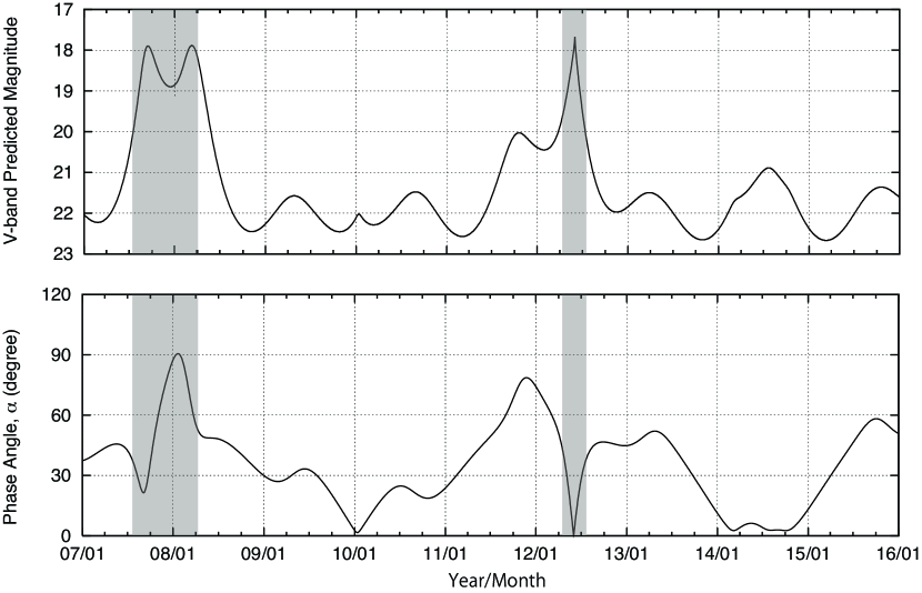
Figure 1: Predicted V magnitude (top) and phase angle (bottom) of JU3 in 2007–2015. There were two observational opportunities in late 2007–early 2008 and late 2011–mid-2012. Note that the magnitude is not the observed value. Although these magnitudes have some degree of uncertainty, they provide a good perspective for understanding the observed condition of the asteroid.

Figure 1 shows the predicted V-band magnitudes and phase angles for given dates in 2007–2016 obtained by NASA/JPL’s Horizons ephemeris generator. The data set in 2007–2008 covers a large phase angle (up to 90°), whereas that in 2011–2012 covers intermediate to low phase angles (down to 0.3°). The combined data thus provide a unique data set for studying the magnitude–phase relation of the C-type asteroid in a wide phase angle range in which main-belt asteroids cannot be observed from earthbound orbit. A worldwide optical observation campaign for JU3 was conducted in 2011–2012 not only to support the Hayabusa 2 project but also to explore the physical nature of the target asteroid. In particular, the campaign gave considerable weight to acquiring the relative magnitudes for deriving the rotational period and shape model (Kim et al., 2013; Kim, 2014). Among the campaign data, we selected magnitude data taken with calibration standard stars under good weather conditions. In addition, we chose data with a substantial signal-to-noise ratio (i.e., S/N $>$ 10) and/or data with even phase angle coverage. We also placed a priority on data at low phase angles. In total, we selected data for JU3 taken on 21 nights with 8 telescopes.

The journal of observations is summarized in Table 1, which includes observations in Kawakami (2009), whose magnitude data were calibrated in a standard manner using photometric standard stars but are not published in any journal. The data we used in this work were taken with the following telescopes and instruments: the University of Hawaii 2.2-m telescope (UH2.2m) with the Tektronix 2048 $\times$ 2048 pixel CCD camera (Tek2k) atop Mauna Kea, USA; the Magellan I 6.5-m Baade telescope (Magellan-1) with the Inamori Magellan Areal Camera and Spectrograph (IMACS); the Magellan II 6.5-m Clay telescope (Magellan-2) with the Low Dispersion Survey Spectrograph (LDSS3) at the Las Campanas Observatory, Chile; the ESO/MPI 2.2-m telescope (ESO/MPI) with the 7-Channel Imager, GROND, at $g^{\prime}$, $r^{\prime}$, $i^{\prime}$, $z^{\prime}$, $J$, $H$, and $K$ (Greiner et al., 2008; Müller et al., 2014) at the La Silla Observatory, Chile; the Nayuta 2.0-m telescope (Nayuta) with the 2048 $\times$ 2064 pixel Multiband Imager (MINT) at the Nishi-Harima Astronomical Observatory, Japan; the Indian Institute of Astrophysics 2.0-m Himalayan Chandra Telescope (HCT) with the Himalayan Faint Object Spectrograph Camera (HFOSC) at the Indian Astronomical Observatory, India; the Tenagra II 0.81-m telescope (Tenagra II) with the 1K $\times$ 1K CCD camera (1KCCD) in Arizona, USA; and the InfraRed Survey Facility 1.4-m telescope (IRSF) with the Simultaneous three-color InfraRed Imager (SIRIUS) (Nagayama et al., 2003) at the South African Astronomical Observatory, South Africa. All but one of these telescopes were operated in a non-sidereal tracking mode, whereas the HCT was operated in a sidereal tracking mode. All the instruments were employed in an imaging mode with the standard broadband astronomical filters listed in Table 1. In addition to these new data taken in 2011–2012, we re-analyzed some of the data taken in 2007 with the 1-m telescope at Lulin Observatory with the 1K $\times$ 1K CCD camera (Taiwan) and the Steward Observatory 1-m telescope in Arizona (USA).

2.2 Pre-processing and Photometry

The observed images were analyzed in the standard way for CCD imaging data. The raw data were subtracted using bias frames (zero exposure) or dark frames (if the instruments were not cooled sufficiently to suppress dark current) that were taken at intervals throughout each night. We used median-stacked data frames using object frames to construct flat-field images with which to correct for vignetting of the optics and pixel-to-pixel variation in the detector’s response. The aperture photometry was conducted using the apphot package in IRAF, which provides the magnitude within synthetic circular apertures projected onto the sky. The parameters for the aperture photometry were determined manually depending on the image quality, but in principle, we set an aperture radius of about 2–3 times the full width at half-maximum (FWHM), which is large enough to enclose the detected flux of the asteroids and standard stars. The sky background was determined within a concentric annulus having projected inner and outer radii of $\sim$3$\times$FWHM and $\sim$4$\times$FWHM for point objects, respectively. Flux calibration was conducted using standard stars in the Landolt catalog for the Johnson-Cousins $B$-, $V$-, $R_{\mathrm{C}}$-, and $I_{\mathrm{C}}$-band filters (Landolt, 1992, 2009); the Sloan Digital Sky Survey (SDSS) catalog for the $g^{\prime}$-, $r^{\prime}$-, $i^{\prime}$-, and $z^{\prime}$-band filters (Ivezić et al., 2007); and the Two Micron All Sky Survey (2MASS) catalog for the $J$-, $H$-, and $K$-band filters (Skrutskie et al., 2006). At Nishi-Harima Astronomical Observatory, the data were taken under variable sky conditions, and the data taken with the Tenagra II and Magellan II were obtained without taking standard star fields. To calibrate these data, we made a follow-up observation of the same sky field with the UH2.2m and the same filter system.

2.3 Derivation of Reduced $V$ Magnitude

As described above, our data were obtained with a variety of filters. To derive the magnitude–phase relation of JU3 using these data, we first examined the color relations among the observed filter bands. The spectra of JU3 at 0.44–0.94 µm has been studied well and shows no rotational variability at the level of a few percent (Moskovitz et al., 2013). We calculated the color indices using the spectrum in Abe et al. (2008), where they combined optical and near-infrared spectra taken at the MMT Observatory and the NASAInfrared Telescope Facility (see also Vilas, 2008; Moskovitz et al., 2013). We considered that the observed asteroid spectrum is a product of the asteroid’s reflectance and the solar spectrum, and calculated the color indices (differences in magnitudes at two different bands) using the following equation:

$$\left(m_{j}-m_{k}\right)=-2.5\log\left(\frac{r_{j}}{r_{k}}\right)+\left(m_{j}-m_{k}\right)_{\odot},$$ (1)

where $r_{j}$ and $r_{k}$ are the reflectances at the effective wavelengths of the $j$-th and $k$-th band filters, respectively, and $\left(m_{j}-m_{k}\right)_{\odot}$ is the color index of the sun between the $j$-th and $k$-th bands. We adopted the color indices of the sun and their uncertainties in Holmberg et al. (2006). We used the formula in Jordi et al. (2006) for converting from the Johnson-Cousins $BVR_{\mathrm{C}}I_{\mathrm{C}}$ system to the SDSS $g^{\prime}r^{\prime}i^{\prime}z^{\prime}$ system. Table 2 compares the observed and calculated color indices. The observed color indices except for $g^{\prime}$-$J$ (taken with GROND) were found to match the calculated color indices to within the accuracy of our measurements ($\sim$5%). We noticed that the $g^{\prime}$ magnitude taken with GROND has an ambiguity in the calibration process due to unstable weather; it seems that the calculated $g^{\prime}$-$J$ color index could be more reliable than the observed one. Hereafter, we adopted the calculated color indices for deriving the corresponding $V$ magnitude and tolerated the uncertainty of 5% associated with the photometric system conversion in the following discussion.

In addition to the phase angle dependence, the observed magnitude of the asteroid changed in time because of its rotation. For JU3, the rotational effect results in a magnitude change no larger than $\sim$0.1 mag with respect to the mean magnitude because it is nearly spherical with an axis ratio of 1.1–1.2 (Kim et al., 2013). To determine the magnitude–phase relation, we corrected the rotational modulation and derived the magnitude averaged over the rotational phase. If observations cover both the peak and the trough, we can derive the mean magnitude as a representative value from a single-night observation. However, because most of the data could not cover a substantial portion of the rotational phase, we may mistake the mean magnitudes. Although the effect is not as large as a half-amplitude of the lightcurve (i.e., 0.1 mag or less), we corrected the rotational effect in 2012 data by deriving the zeroth-order term from the nightly data using an empirical Fourier model to describe the relative magnitude change due to the rotation of JU3. It is given by the following fourth-order Fourier series (Kim, 2014):

$$\Phi\left(t\right)=\sum_{h=1}^{4}\left[A_{2h-1}\sin\left(2\pi fh(t_{JD}-t_{0})\right)+A_{2h}\cos\left(2\pi fh(t_{JD}-t_{0})\right)\right]~{}~{},$$ (2)

where $\Phi(t)$ denotes the relative magnitude change caused by the rotation of JU3, $f$ = 3.1475 is the rotational frequency in day^-1, and $t_{JD}$ and $t_{0}=$ 2456106.834045 (08:01:01.49 UT on 2012 June 28) are the observed median time in Julian days and offset time for phase zero (see Figure 1 in Kim et al., 2013), respectively. $A_{2h-1}$ and $A_{2h}$ are constants given by $A_{1}$ = 0.0067, $A_{2}$ = 0.030, $A_{3}$ = 0.010, $A_{4}$ = 0.055, $A_{5}$ = 0.031, $A_{6}$ = 0.019, $A_{7}$ = 0.0070, and $A_{8}$ = 0.0033. Assuming the observed magnitudes are given by $\Phi(t)+H_{\mathrm{V}}(\alpha)$, we fitted the observed magnitudes after color correction using Eq. (2) and derived the inferred mean magnitudes, $H_{\mathrm{V}}(\alpha)$. To evaluate how well the empirical lightcurve model reproduces the observed lightcurve, we compared the model in Eq. (2) with lightcurve data taken at several different nights in 2012; these include light curves taken on 2012 May 31 with MOA-cam3 attached to MOA-II telescope at Mt. John Observatory, New Zealand (Sako et al., 2008; Sumi et al., 2010), and on 2012 July 17–19 with HCT. We found that the deviation is no larger than a few percent. We considered a 4% uncertainty associated with the correction for the lightcurve. Regarding 2007–2008 data, the lightcurve model may not applicable because of the long interval of time between $t_{JD}$ and $t_{0}$. We adopted the observed mean magnitudes and considered a 10% uncertainty.

The observed corresponding $V$ magnitude, $H_{\mathrm{V}}(\alpha)$, was converted into the reduced V magnitude $H_{\mathrm{V}}(1,1,\alpha)$, a magnitude at a hypothetical position in the solar system, that is, a heliocentric distance $r_{h}$ = 1 AU, an observer’s distance of $\Delta$ = 1 AU, and a solar phase angle $\alpha$, which is given by

$$H_{\mathrm{V}}(1,1,\alpha)=H_{\mathrm{V}}(r_{h},\Delta,\alpha)-5~{}\log(r_{h}\Delta)~{}~{}.$$ (3)

3 Results

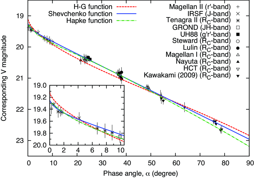
Figure 2: Magnitude–phase relation of JU3. All observed magnitudes were converted into corresponding V magnitudes assuming the color of the asteroid in Table 2 at a hypothetical position of 1 AU from the sun and observer. We show three models, that is, IAU $H$–$G$ function with our best fit parameters, $H_{\mathrm{V}}$ = 19.13 $\pm$ 0.03 and $G$ = $-0.006\pm$ 0.012, Shevchenko function with the best fit parameters, $a$ = 0.21 $\pm$ 0.04, $b$ = 0.039 $\pm$ 0.001, and $H_{\mathrm{V}}$ = 19.24 $\pm$ 0.03, and Hapke model with one of the best fit parameter sets, $\bar{\theta}=20$°, $w=0.041$, $g=-0.38$, $B_{0}=1.43$, and $h=0.050$.

In Figure 2, we show the magnitude–phase relation. It shows obvious phase darkening, which is commonly observed in small solar system bodies. The photometric calibration and color index correction appeared to work well, not only because our new data set is smoothly connected to data from Kawakami (2009), but also because there is no systematic displacement according to the observed filters. In the following subsections, we apply three photometric functions to characterize the magnitude–phase relation of JU3. For the fitting, we employed the Levenberg–Marquardt algorithm to iteratively adjust the parameters to obtain the minimum value of $\chi^{2}$, which is defined as

$$\chi^{2}=\frac{1}{N}\sum^{N}_{n=1}\left[H_{\mathrm{V}}(1,1,\alpha)-\mathcal{H}_{\mathrm{V}}(1,1,\alpha)\right]^{2},$$ (4)

where $\mathcal{H}_{\mathrm{V}}(1,1,\alpha)$ is the reduced magnitude calculated by each model. $N$ is the number of magnitude data points. The observed data points are weighted by $\sigma H_{\mathrm{V}}(1,1,\alpha)^{-2}$ for the fitting, where $\sigma H_{\mathrm{V}}(1,1,\alpha)$ denotes the error of reduced magnitude.

3.1 IAU $H$–$G$ formalism fitting

We initially applied the $H$–$G$ formalism described in Lumme et al. (1984) and Bowell et al. (1989). The function was adopted by the International Astronomical Union (IAU) and has been widely used as a standard asteroid phase curve. It has the mathematical form

$$\mathcal{H}_{\mathrm{V}}(1,1,\alpha)=H_{\mathrm{V}}-2.5\log\left[\left(1-G\right)\exp\left(-3.33\tan^{0.63}(\alpha/2)\right)+G\exp\left(-1.87\tan^{1.22}(\alpha/2)\right)\right]~{},$$ (5)

where $H_{\mathrm{V}}$ is the absolute magnitude in the V band, and $G$ is the slope parameter indicative of the steepness of the phase curve. By fitting the entire data set, we obtained values of $H_{\mathrm{V}}$ = 19.12 $\pm$ 0.03 and $G$ = $-0.03$ $\pm$ 0.01 (dashed line in Figure 2). A careful examination of the fitting results reveals that two-parameter fitting with the $H$–$G$ formalism cannot fit the entire magnitude–phase relation, causing a discrepancy in the absolute magnitude. The fitting does not match the observational magnitude at small phase angles ($\alpha$ $<$ 2°). In addition, the obtained slope parameter $G$ takes a peculiar negative value, although asteroids usually take positive values (Harris, 1989). Because the $H$–$G$ formalism has been usually applied for main-belt asteroids observed at $\alpha\lesssim 30$, we fitted the data at $\alpha$ $<$ 30°. We obtained values of $H_{\mathrm{V}}$ = 19.22 $\pm$ 0.02 and $G$ = 0.13 $\pm$ 0.02. We obtained the moderate $G$ value this time, although the model is largely deviated from the observed data at $\alpha>$40°.

3.2 Shevchenko function fitting

A simple but judicious model was proposed by Shevchenko (1996) for approximating an asteroid’s magnitude–phase curves. It has the form

$$\mathcal{H}_{\mathrm{V}}(1,1,\alpha)=C-\frac{a}{1+\alpha}+b~{}\alpha~{}~{},$$ (6)

where $a$ is a parameter that characterizes the opposition effect amplitude, and $b$ is a slope (mag deg^-1) describing the linear part of the phase dependence. $C$ is given by $C$ = $H_{\mathrm{V}}+a$. By fitting the entire data set, we obtained $H_{\mathrm{V}}$ = 19.24 $\pm$ 0.03, $a$ = 0.19 $\pm$ 0.04, and $b$ = 0.039 $\pm$ 0.001 mag deg^-1. It is interesting to notice that the Shevchenko function fits the observed data in a wide phase angle range from 0.3° to 75°, although it was contrived to fit observed data at small phase angles (i.e. $\alpha<$40°). We obtained an absolute magnitude close to that obtained by the $H$–$G$ formalism for the data at $\alpha<$30°.

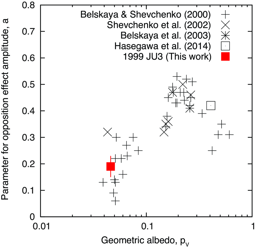
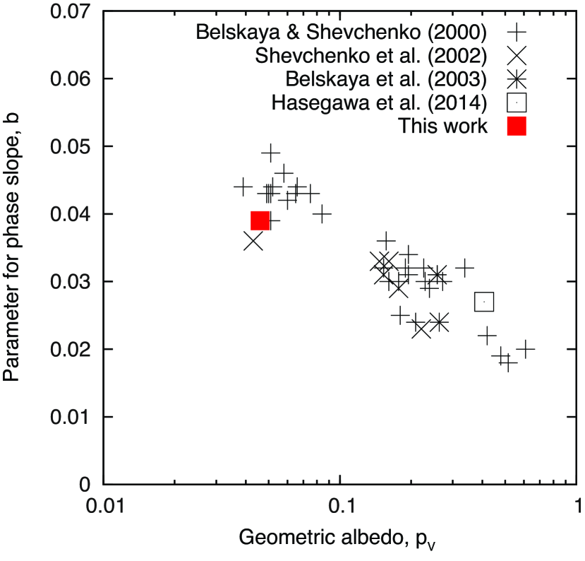
Figure 3: Geometric albedo dependences of parameters for the opposition effect amplitude and linear phase slope in Shevchenko’s function. The original data were obtained from Belskaya & Shevchenko (2000), Shevchenko et al. (2002), Belskaya et al. (2003), and Hasegawa et al. (2014). We updated the albedo values using data in Usui et al. (2011).

The Shevchenko function has an advantage in that it provides a direct derivation of the opposition effect amplitude. With the best fit parameter of $a$ and $b$, we computed the reflectance ratio of $I(0.3\arcdeg)$/$I(5\arcdeg)$ = 1.31 $\pm$ 0.05, where $I(0.3\arcdeg)$ and $I(5\arcdeg)$ are the reflectances at $\alpha$ = 0.3° and $\alpha$ = 5°, respectively. Figure 3 shows the albedo dependence of parameters for the opposition effect amplitude and linear phase slope of JU3, which are compared with those of $\gtrsim$10-km asteroids (Belskaya & Shevchenko, 2000; Shevchenko et al., 2002; Belskaya et al., 2003; Hasegawa et al., 2014). As noted in Belskaya & Shevchenko (2000), the phase slope increases linearly as the albedo decreases. They provided a phenomenological model to relate the phase slope and the geometric albedo. Applying their empirical law, we obtained a geometric albedo of 0.08 $\pm$ 0.03. The albedo is in accordance with the geometric albedo of JU3 (see below). The consistency of the phase slopes and the opposition effect amplitudes between $\gtrsim$10-km asteroids and sub-km asteroid JU3 may suggest that the magnitude–phase relation would be dominated by the albedo, not by the asteroid diameter. The amplitude and width of the opposition effect are considered to represent the distance from the sun theoretically (Déau, 2012). The effect is caused by the apparent size of the sun when viewed from asteroids. JU3 was observed at a solar distance of $r_{h}$ = 1.36 AU, whereas the other asteroids in Figure 3 were observed at $r_{h}$ = 1.8–3.4 AU. No significant difference is found between JU3 and the other dark asteroids, most likely because the error is not small enough to detect such a solar distance effect.

3.3 Hapke model fitting

Finally, we employed the Hapke model (Hapke, 1981, 1984, 1986). It has been applied to in-situ observational data taken with spacecraft onboard cameras. The Hapke model provides an excellent approximation of the photometric function to correct for different illumination conditions. However, because it has a complicated mathematical form with many parameters (typically five or six), it often does not give a unique fit to the limited observational data (Helfenstein & Veverka, 1989; Belskaya & Shevchenko, 2000). Some parameters are correlated with others to compensate one another, so there are a number of best-fit parameter sets. Despite this complexity, the application of the Hapke model is attractive in preparation for in-situ observation by Hayabusa 2.

The observed corresponding V magnitudes are converted into the logarithm of $I/F$ (where $F$ is the incidence solar irradiance divided by $\pi$, and $I$ is the intensity of reflected light from the asteroid surface) as

$$-2.5\log\left(\frac{I}{F}\right)=\mathcal{H}_{\mathrm{V}}(1,1,\alpha)-m_{V\odot}-\frac{5}{2}\log\left(\frac{\pi}{S}\right)+m_{c}~{}~{},$$ (7)

where $m_{V\odot}$ is the V-band magnitude of the sun at 1 AU, $S$ is the geometrical cross section of JU3 in m², and $m_{c}$ = $-5\log(1.4960\times 10^{11})$ = $-55.87$ is a constant to adjust the length unit. We used $m_{V\odot}$ = $-26.74$ (Allen, 1973). We took the apparent cross section of JU3 $S$ = (5.94 $\pm$ 0.27) $\times$ 10⁵ m², which is the equivalent area of a circle with a diameter of 870 $\pm$ 10 m (Müller et al., 2014). The original Hapke model was contrived to characterize the bidirectional reflectance of airless bodies (Hapke, 1981). However, the observed quantity in this paper is the magnitude integrated over the sunlit hemisphere observable from ground-based observatories. We adopted the Hapke function integrating the intensity per unit area over that portion of a spherical body (Hapke, 1984). The equation is given as

$$\frac{I}{F}=\left[\left(\frac{w}{8}\left[\left(1+B(\alpha)\right)P(\alpha)-1\right]+\frac{r_{0}}{2}(1-r_{0})\right)\left(1-\sin\left(\frac{\alpha}{2}\right)\tan\left(\frac{\alpha}{2}\right)\ln\left[\cot\left(\frac{\alpha}{4}\right)\right]\right)\right.$$

$$\left.+\frac{2}{3}r_{0}^{2}\left(\frac{\sin(\alpha)+(\pi-\alpha)\cos(\alpha)}{\pi}\right)\right]K(\alpha,\bar{\theta})~{}~{},$$ (8)

where $w$ is the single-particle scattering albedo. $K(\alpha,\bar{\theta})$ is a function that corrects for the surface roughness parameterized by $\bar{\theta}$ (Hapke, 1984). The term $r_{0}$ is given by

$$r_{0}=\frac{1-\sqrt{1-w}}{1+\sqrt{1-w}}~{}~{}.$$ (9)

The opposition effect term $B(\alpha)$ is given by

$$B(\alpha)=\frac{B_{0}}{1+\frac{\tan(\alpha/2)}{h}}~{}~{},$$ (10)

where $B_{0}$ characterizes the amplitude of the opposition effect, and $h$ characterizes the width of the opposition effect. We used the one-term Henyey–Greenstein single particle phase function solution (Henyey & Greenstein, 1941):

$$P(\alpha)=\frac{(1-g^{2})}{(1+2g\cos(\alpha)+g^{2})^{3/2}}~{}~{},$$ (11)

where $g$ is called the asymmetry factor. Positive values of $g$ indicate forward scatter, $g$=0 isotropic, and negative $g$ backward scatter.

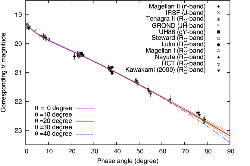
Figure 4: Comparison between five sets of Hapke model parameters in Table 3 ($\bar{\theta}=$0–40° from top to bottom).

For the fitting, we considered initial values in the possible ranges of the parameters, that is, $0.01\leq w\leq 0.09$ at intervals of 0.02, $0.01\leq h\leq 0.1$ at intervals of 0.03, $-0.5\leq g\leq-0.1$ at intervals of 0.2, $0\leq B_{0}\leq 4.0$ at intervals of 1, and $0\arcdeg\leq\bar{\theta}\leq 40\arcdeg$ at intervals of 10°, and conducted the parameter fitting. However, we soon realized that the fitting algorithm cannot converge when these five parameters are variables. We found that, mathematically, the effect of the surface roughness, $\bar{\theta}$, can be compensated by the other parameters to produce nearly identical disk-integrated curves; consequently, the fitting algorithm cannot converge. A similar argument was made for Itokawa’s disk-integrated function, where it was claimed that high phase angle data are necessary to constrain the surface roughness effect (Lederer et al., 2008). We assumed $\bar{\theta}$ to be 0°, 10°, 20°, 30°, or 40° and derived the other parameters for the given $\bar{\theta}$ values. The obtained Hapke parameters are summarized in Table 3 and the magnitude–phase relation with the parameters is shown in Figure 2 and Figure 4. In terms of $\chi^{2}$, there is no significant difference between the models with different $\bar{\theta}$. However, our magnitude data at high phase angles favour models with $\bar{\theta}\lesssim$30°(see Figure 4 at $\alpha>$70°).

In Table 3, we calculated the Bond albedo (also known as the spherical albedo), $A_{B}$, which is the fraction of incident light scattered in all directions by the surface. It is given by $A_{B}$ = $qp_{\mathrm{V}}$, where $q$ is the value of the phase integral, defined as

$$q=2\int_{0}^{\pi}\frac{\Phi(\alpha)}{\Phi(0)}~{}\sin(\alpha)~{}d\alpha~{}~{}.$$ (12)

In comparison with the other mission target asteroids, JU3 has Hapke parameters similar to those of the C-type asteroid Mathilde. We noticed that the resultant albedos are independent of the surface roughness, although the other Hapke parameters depend on the assumed roughness. The Hapke model matches well Shevchenko’s model at the lowest phase angle, yielding $H_{\mathrm{V}}$ = 19.24 $\pm$ 0.03. From the absolute magnitude, we can conclude that JU3 has a geometric albedo of $p_{\mathrm{V}}$ = 0.046 $\pm$ 0.004. The derived albedo is consistent with those of C-type asteroids, that is, 0.071$\pm$0.040 (Usui et al., 2013).

4 Discussion

4.1 Error Analysis

As we described above, we considered possible error sources with conservative estimates and obtained the total error. Eventually, each corresponding V magnitude has a photometric error of $\sim$0.1 mag. The photometric models above fit the observed data within the photometric errors, most likely because we may give adequate consideration to the errors. As a result, each error in the magnitude data taken with a variety of filters and instruments seems to be randomized, which provides a reliable absolute magnitude. We obtained a fitting error of the absolute magnitude of 0.03 mag. It is important to note that the absolute magnitude we derived differs greatly (0.4 mag) from that in the previous study (Kawakami, 2009), which was obtained on the basis of observation at $\alpha>$ 22° and is commonly referred to in previous research to derive the geometric albedo (Hasegawa et al., 2008; Campins et al., 2009; Müller et al., 2011). In general, the absolute magnitudes of main-belt asteroids have been determined through ground-based observations at $\alpha<30$°. It is likely that Kawakami (2009) might lead inadequate result in the absolute magnitude due to the paucity of data at low phase angles. Because our data set covers low phase angles almost equivalent to half of the apparent solar disk size, it provides a more reliable absolute magnitude without extrapolating the phase function.

A drawback of our measurement is that we ignored the wavelength dependence of the magnitude–phase relation. In fact, the single scattering albedo ($w$) and opposition surge width ($h$) of S-type asteroids Itokawa and Eros exhibit strong wavelength dependences (Kitazato et al., 2008; Clark et al., 1999). Figure 2 shows the magnitude–phase relation for the various filters. In particular, we have $J$-band and $R_{\mathrm{C}}$-band data at $\alpha<$ 10°. Because the phase slopes of these two bands are nearly the same, we conjecture that the magnitude–phase relation is less dependent on the wavelength. In general, the observed magnitude–phase relation can be influenced by a combination of the shadow-hiding effect and coherent backscattering mechanism, and these effects depend on the geometric albedo (Belskaya & Shevchenko, 2000). Unlike Itokawa and Eros, which have very red spectra with moderate absorption around 1 µm, JU3 has almost constant reflectance from 0.45 µm to $\sim$1.5 µm  (Moskovitz et al., 2013). Accordingly, we may attribute the weak wavelength dependence of the phase curve to the flat spectrum of JU3.

Regarding the errors of the Hapke parameters, a large uncertainty remains because of the undetermined $\bar{\theta}$. The $\chi^{2}$ derived by Shevchenko’s function is equivalent to that derived by the Hapke function, suggesting that three-parameter fitting for Shevchenko’s function is mathematically sufficient to characterize the observed magnitude–phase relation. We fixed the surface roughness parameter $\bar{\theta}$ and derived the other four parameters in the Hapke model. It seems that $B$ and $h$ characterize the shape and amplitude of the opposition effect, which correspond to a parameter, $a$, in Shevchenko’s function, whereas the other two parameters adjust the vertical magnitude offset and the entire phase slope, which correspond to $H_{\mathrm{V}}$ and $b$ in Shevchenko’s function. Among the Hapke parameters, we determined $h$ independently of $\bar{\theta}$. $h$ can be interpreted in terms of porosity and grain size of the optically active regolith. Applying a model in Hapke (1986) and assuming a lunar-like grain size distribution with a ratio of the largest particle size to the smallest particle size of 10³, we obtained the porosity of 0.64. The derived porosity suggests that the surface of JU3 may be covered with coarse regoliths ($\approx$1 cm, using an empirical size–porosity relation in Kiuchi & Nakamura 2014).

4.2 In Preparation for the Hayabusa 2 Mission

The primary goal of the Hayabusa 2 mission is to bring back samples from a C-type asteroid or an asteroid analogous to C-type asteroids, following up on the Hayabusa 1 mission, which returned a sample from the S-type asteroid Itokawa (Yoshikawa et al., 2008, 2012). Because of the similarity of the spectra, C-type asteroids are considered to be parent bodies of carbonaceous chondrite meteorites, which are abundant in organic materials and hydrous minerals. In the nominal plan, multiple samplings are scheduled to obtain different types of asteroid material on the basis of their composition and degrees of aqueous alteration and space weathering. Because the reflectance at 0.55 µm depends mainly on the abundance of carbon compounds, the surface reflectance map will provide information useful for the selection of the sampling sites. Therefore, speedy construction of the reflectance map is crucial to the project’s success. The observed reflectances at given wavelengths should be converted to a standard geometry consisting of the incident angle $i$ = 30°  emission angle $e$ = 0°, and phase angle $\alpha$ = 30° using a photometric model. Among the models, the Hapke model has been widely used to correct data taken with spacecraft onboard cameras (see, e.g., Clark et al., 1999, 2002). Through this work, we have determined the Hapke parameters except for the surface roughness. Because the disk-resolved reflectance is sensitive to the surface roughness, we expect that it will be obtained uniquely once the JU3 images are taken. We thus propose to determine the surface roughness while fixing the other four parameters on a restricted basis by the magnitude–phase relation. The construction of JU3’s shape model is essential to calculating the incident and emission angles. Once the shape is determined, we expect that the full set of Hapke parameters will be fixed using the images taken with the onboard cameras.

Our work provides useful information for the calibration of the onboard remote-sensing devices such as the Optical Navigation Camera (ONC) and the Deployable CAMera (DCAM). Specifically, we provide accurate magnitude models. Similar to the procedure on the Hayabusa 1 mission, measurements of JU3’s lightcurve are planned for the purpose of flux calibration (Sugita et al., 2013). A comparison of the magnitude–phase relation in this paper and the observed disk-integrated data count will enable the determination of the calibration factors, as we did using stellar observations during the cruising phase for Hayabusa Asteroid Multi-band Imaging Camera (AMICA) (Ishiguro et al., 2010). Unlike the case of AMICA for Hayabusa 1, we expect that the calibration parameters will be determined easily thanks to the accurate photometric models in this paper.

5 Summary

We examined the magnitude–phase relation of (162173) 1999 JU3 using data taken from ground-based observatories. The major findings of this paper are as follows:

1. The IAU $H$–$G$ formalism does not fit the observed data at small and large phase angles ($\alpha$ $<$ 2° and $\alpha$ $>$ 50°) simultaneously using a single set of parameters. By fitting the data set at $\alpha$ $<$ 30°, we obtained values of $H_{\mathrm{V}}$ = 19.22 $\pm$ 0.02 and $G$ = 0.13 $\pm$ 0.02.

2. Using the Shevchenko function, we found that the magnitude–phase relation exhibits linear behavior in a wide range of phase angles ($\alpha$ = 5–75°) and shows weak nonlinear opposition brightening at $\alpha<$ 5°. The phase slope (0.039 $\pm$ 0.001 mag deg^-1) and opposition effect amplitude (parameterized by the ratio of intensity at $\alpha$=0.3° to that at $\alpha$=5°, $I(0.3\arcdeg)$/$I(5\arcdeg)$=1.31$\pm$0.05) are consistent with those of typical C-type asteroids.

3. We were not able to uniquely constrain the full set of parameters in the Hapke model, but were able to find the best-fit values for four parameters given a range of fixed values for the surface roughness parameter. Assuming $\bar{\theta}$=20°(the typical value for C-type asteroids, Clark et al. (1999)), we obtained $w$=0.041, $g$=-0.38, $B_{0}$=1.43, and $h$=0.050. The results obtained are consistent with those of the C-type asteroid Mathilde.

4. By combining this study with a thermal model of asteroids (Müller et al. in preparation), we obtained a geometric albedo of $p_{\mathrm{v}}$ = 0.047 $\pm$ 0.003, a phase integral of $q$ = 0.32 $\pm$ 0.03, and a Bond albedo of $A_{\mathrm{B}}$ = 0.014 $\pm$ 0.002.

Acknowledgments
This research was supported by the Korea Research Council of Fundamental Science & Technology and by the Korea Astronomy and Space Science Institute. We would like to thank the referee, Dr. Bruce Hapke, for carefully reading our manuscript and for giving constructive comments. This paper was written when the first author was at UCLA and Paris Observatory, where he was supported by Prof. David Jewitt and Dr. Jeremie Vaubaillon. SH was supported by the Space Plasma Laboratory, ISAS, JAXA. Part of the funding for GROND (both hardware as well as personnel) was generously granted from the Leibniz-Prize to Prof. G. Hasinger (DFG grant HA 1850/28-1). P.S. acknowledges support by DFG grant SA 2001/1-1.

Table 1: Observation Summary

Telescope	Instrument	Filter	Date (UT)
This work
UH2.2m	Tek2048	$r^{\prime}$, $g^{\prime}$	2012 June 26, 27, July 12
IRSF	SIRIUS	$J$, $H$, $K$	2012 May 30, 31, June 1, 2, 4
Magellan I	IMACS	$R_{\mathrm{C}}$	2012 April 5–7
Magellan II	LDSS3	$g^{\prime}$, $r^{\prime}$, $i^{\prime}$	2012 June 1
ESO/MPI	GROND	$g^{\prime}$, $r^{\prime}$, $i^{\prime}$, $z^{\prime}$, $J$, $H$, $K$	2012 May 28, June 9–10
Tenagra II	SITe 1k CCD	$R_{\mathrm{C}}$	2012 May 31, June 7–9
Nayuta	MINT	$R_{\mathrm{C}}$	2012 June 22
HCT	HFOSC	$R_{\mathrm{C}}$	2012 July 17
Steward	Optical CCD	$V$, $R_{\mathrm{C}}$	2007 September 10–13
Lulin	EEV 1k CCD	$B$, $V$, $R_{\mathrm{C}}$, $I_{\mathrm{C}}$	2007 July 19–23, December 3, 7–8
			2008 February 27–28, April 2, 4–5
Kawakami (2009)
Kiso	2KCCD	$B$, $V$, $R_{\mathrm{C}}$	2007 November 8

Table 2: Color Indices

	$B$-$V$	$V$-$R_{\mathrm{C}}$	$V$-$I_{\mathrm{C}}$	$g^{\prime}$-$r^{\prime}$	$r^{\prime}$-$i^{\prime}$	$V$-$J$	$g^{\prime}$-$J$
Observed(Kawakami, 2009)	0.66 (0.06)	0.40 (0.06)	0.74 (0.07)	–	–	–
Observed (this work)		0.37 (0.03)	–	0.47 (0.03)	–	–	1.16 (0.05)
Calculated	0.65 (0.01)	0.34 (0.01)	0.72 (0.01)	0.45 (0.02)	0.13 (0.01)	1.21 (0.04)	1.48 (0.05)

Table 3: Hapke Parameters for JU3 and Other Mission Target Asteroids in V Band (550 nm)

	Typea	$w^{b}$	$g^{c}$	$\bar{\theta}^{d}$ (°)	$B_{0}^{e}$	$h^{f}$	$p_{\mathrm{V}}^{g}$	$q^{h}$	$A_{\mathrm{B}}^{i}$	Reference
This work
1999 JU3	Cg	0.038	-0.39	[0]	1.52	0.049	0.045	0.32	0.014	$\cdots$
		0.039	-0.39	[10]	1.49	0.049	0.045	0.32	0.014	$\cdots$
		0.041	-0.38	[20]	1.43	0.050	0.045	0.31	0.014	$\cdots$
		0.046	-0.36	[30]	1.34	0.051	0.045	0.31	0.014	$\cdots$
		0.052	-0.34	[40]	1.21	0.051	0.044	0.30	0.013	$\cdots$
Other mission targets
(253) Mathilde	Cb	0.035	-0.25	19	3.18	0.074	0.041	0.33	0.013	Clark et al. (1999)
(243) Ida	S	0.22	-0.33	18	1.53	0.02	0.21	0.34	0.070	Helfenstein et al. (1996)
(433) Eros	S	0.43	–	36	1.0	0.022	0.29	0.39	0.12	Domingue et al. (2002)
(951) Gaspra	S	0.36	-0.18	29	1.63	0.06	0.22	0.49	0.11	Helfenstein et al. (1994)
(25143) Itokawa	Sk	0.70	–	40	0.02	0.141	0.19	0.11	0.021	Lederer et al. (2008)
(5535) Annefrank	S	0.63	-0.09	49	[1.32]	0.015	0.28	0.44	0.12	Hillier et al. (2011)
(4) Vesta	V	0.51	-0.24	18	1.83	0.048	0.42	0.47	0.20	Li et al. (2013); Hasegawa et al. (2014)
(2867) Steins	E	0.66	-0.30	28	0.60	0.027	0.39	0.59	0.24	Spjuth et al. (2012)∗

Note. — Numbers in the parentheses are errors of the color indices.

Note. — ^a Taxonomic type, ^b Single-scattering albedo, ^c Asymmetry factor, ^d Roughness parameter, ^e Opposition amplitude parameter, ^f Opposition width parameter, ^g Geometric albedo, ^h Phase integral, and ⁱ Bond albedo. ^∗ Parameters obtained at 630 nm.

Numbers in parentheses for $\bar{\theta}$ are fixed values.

References

- Abe et al. (2008) Abe, M., Kawakami, K., Hasegawa, S., et al. 2008, Lunar and Planetary Institute Science Conference Abstracts, 39, 1594
- Allen (1973) Allen, C. W. 1973, London: University of London, Athlone Press, —c1973, 3rd ed.,
- Belskaya & Shevchenko (2000) Belskaya, I. N., & Shevchenko, V. G. 2000, Icarus, 147, 94
- Binzel et al. (2001) Binzel, R. P., Harris, A. W., Bus, S. J., & Burbine, T. H. 2001, Icarus, 151, 139
- Belskaya et al. (2003) Belskaya, I. N., Shevchenko, V. G., Kiselev, N. N., et al. 2003, Icarus, 166, 276
- Bowell et al. (1989) Bowell, E., Hapke, B., Domingue, D., et al. 1989, Asteroids II, 524
- Bus & Binzel (2002) Bus, S. J., & Binzel, R. P. 2002, Icarus, 158, 146
- Campins et al. (2009) Campins, H., Emery, J. P., Kelley, M., et al. 2009, A&A, 503, L17
- Campins et al. (2012) Campins, H., de León, J., Morbidelli, A., et al. 2012, LPI Contributions, 1667, 6452
- Clark et al. (1999) Clark, B. E., et al. 1999, Icarus, 140, 53
- Clark et al. (2002) Clark, B. E., Helfenstein, P., Bell, J. F., et al. 2002, Icarus, 155, 189
- Cloutis et al. (2011) Cloutis, E. A., Hiroi, T., Gaffey, M. J., Alexander, C. M. O’D., & Mann, P. 2011, Icarus, 212, 180
- Déau (2012) Déau, E. 2012, J. Quant. Spec. Radiat. Transf., 113, 1476
- Domingue et al. (2002) Domingue, D. L., Robinson, M., Carcich, B., Joseph, J., Thomas, P., & Clark, B. E. 2002, Icarus, 155, 205
- Gradie & Tedesco (1982) Gradie, J., & Tedesco, E. 1982, Science, 216, 1405
- Greiner et al. (2008) Greiner, J., Bornemann, W., Clemens, C., et al. 2008, PASP, 120, 405
- Hapke (1981) Hapke, B. 1981, J. Geophys. Res., 86, 3039
- Hapke (1984) Hapke, B. 1984, Icarus, 59, 41
- Hapke (1986) Hapke, B. 1986, Icarus, 67, 264
- Hapke (1993) Hapke, B. 1993, Topics in Remote Sensing, Cambridge, UK: Cambridge University Press
- Harris (1989) Harris, A. W. 1989, Lunar and Planetary Institute Science Conference Abstracts, 20, 375
- Hasegawa et al. (2008) Hasegawa, S., Müller, T. G., Kawakami, K., et al. 2008, PASJ, 60, 399
- Hasegawa et al. (2014) Hasegawa,S., Miyasaka, S., Tokimasa, N., Sogame, A., Ibrahimov, M. A., Yoshida, F., Ozaki, S., Abe, M., Ishiguro, M., Kuroda, D., 2014, PASJ(accepted on June 18, 2014)
- Helfenstein & Veverka (1989) Helfenstein, P., & Veverka, J. 1989, Asteroids II, 557
- Helfenstein et al. (1994) Helfenstein, P., et al. 1994, Icarus, 107, 37
- Helfenstein et al. (1996) Helfenstein, P., et al. 1996, Icarus, 120, 48
- Henyey & Greenstein (1941) Henyey, L. G., & Greenstein, J. L. 1941, ApJ, 93, 70
- Hillier et al. (2011) Hillier, J. K., Bauer, J. M., & Buratti, B. J. 2011, Icarus, 211, 546
- Holmberg et al. (2006) Holmberg, J., Flynn, C., & Portinari, L. 2006, MNRAS, 367, 449
- Ishiguro et al. (2010) Ishiguro, M., Nakamura, R., Tholen, D. J., et al. 2010, Icarus, 207, 714
- Ivezić et al. (2007) Ivezić, Ž., Smith, J. A., Miknaitis, G., et al. 2007, AJ, 134, 973
- Johnson & Fanale (1973) Johnson, T. V., & Fanale, F. P. 1973, J. Geophys. Res., 78, 8507
- Jordi et al. (2006) Jordi, K., Grebel, E. K., & Ammon, K. 2006, A&A, 460, 339
- Kawakami (2009) Kawakami, K. 2009, Master’s thesis, University of Tokyo
- Kiuchi & Nakamura (2014) Kiuchi, M. and Nakamura, A. M. 2014, Icarus (in press)
- Kim et al. (2013) Kim, M.-J., Choi, Y.-J., Moon, H.-K., et al. 2013, A&A, 550, L11
- Kim (2014) Kim, M. J. 2014, Doctoral thesis, Yonsei University
- Kitazato et al. (2008) Kitazato, K., Clark, B. E., Abe, M., et al. 2008, Icarus, 194, 137
- Landolt (1992) Landolt, A. U. 1992, AJ, 104, 1, 340
- Landolt (2009) Landolt, A. U. 2009, AJ, 137, 4186
- Lazzaro et al. (2013) Lazzaro, D., Barucci, M. A., Perna, D., et al. 2013, A&A, 549, L2
- Lederer et al. (2008) Lederer, S. M., Domingue, D. L., Thomas-Osip, J. E., Vilas, F., Osip, D. J., Leeds, S. L., & Jarvis, K. S. 2008, Earth, Planets, and Space, 60, 49
- Li et al. (2013) Li, J.-Y., Le Corre, L., Schröder, S. E., et al. 2013, Icarus, 226, 1252
- Lumme et al. (1984) Lumme, K., Bowell, E., & Harris, A. W. 1984, BAAS, 16, 684
- Moskovitz et al. (2013) Moskovitz, N., Abe, S., Pan, K.-S., et al. 2013, arXiv:1302.1199
- Mothé-Diniz et al. (2003) Mothé-Diniz, T., Carvano, J. M. Á., & Lazzaro, D. 2003, Icarus, 162, 10
- Müller et al. (2011) Müller, T. G., Ďurech, J., Hasegawa, S., et al. 2011, A&A, 525, A145
- Müller et al. (2014) Müller, T. G. et al. in preparation
- Nagayama et al. (2003) Nagayama, T., Nagashima, C., Nakajima, Y., et al. 2003, Proc. SPIE, 4841, 459
- Pinilla-Alonso et al. (2013) Pinilla-Alonso, N., Lorenzi, V., Campins, H., de Leon, J., & Licandro, J. 2013, A&A, 552, A79
- Rieke et al. (2008) Rieke, G. H., Blaylock, M., Decin, L., et al. 2008, AJ, 135, 2245
- Sako et al. (2008) Sako, T., Sekiguchi, T., Sasaki, M., et al. 2008, Experimental Astronomy, 22, 51
- Shevchenko (1996) Shevchenko, V. G. 1996, Lunar and Planetary Institute Science Conference Abstracts, 27, 1193
- Shevchenko et al. (2002) Shevchenko, V. G., Belskaya, I. N., Krugly, Y. N., Chiomy, V. G., & Gaftonyuk, N. M. 2002, Icarus, 155, 365
- Shevchenko et al. (2012) Shevchenko, V. G., Belskaya, I. N., Slyusarev, I. G., et al. 2012, Icarus, 217, 202
- Skrutskie et al. (2006) Skrutskie, M. F., Cutri, R. M., Stiening, R., et al. 2006, AJ, 131, 1163
- Spjuth et al. (2012) Spjuth, S., Jorda, L., Lamy, P. L., Keller, H. U., & Li, J.-Y. 2012, Icarus, 221, 1101
- Sugita et al. (2013) Sugita, S., Kuroda, D., Kameda, S., et al. 2013, LPI Contributions, 1719, 2591
- Sumi et al. (2010) Sumi, T., Bennett, D. P., Bond, I. A., et al. 2010, ApJ, 710, 1641
- Usui et al. (2011) Usui, F., Kuroda, D., Müller, T. G., et al. 2011, PASJ, 63, 1117
- Usui et al. (2013) Usui, F., Kasuga, T., Hasegawa, S., et al. 2013, ApJ, 762, 56
- Vilas (2008) Vilas, F. 2008, AJ, 135, 1101
- Wasson & Kallemeyn (1988) Wasson, J. T., & Kallemeyn, G. W. 1988, Royal Society of London Philosophical Transactions Series A, 325, 535
- Yoshikawa et al. (2012) Yoshikawa, M., Minamino, H., Tsuda, Y., et al. 2012, LPI Contributions, 1667, 6188
- Yoshikawa et al. (2008) Yoshikawa, M., Yano, H., Kawaguchi, J., Hayabusa-2 Pre-Project Team, & Small Body Exploration WG 2008, Lunar and Planetary Institute Science Conference Abstracts, 39, 1747